1. Introduction
Precipitation has a significant impact on various aspects such as ecology, environment, and climate, and accurate prediction of precipitation is therefore of great importance for social and economic development. However, due to the high randomness and uncertainty of precipitation, precipitation forecasting has always been a highly challenging issue. In order to improve the accuracy of precipitation prediction, researchers have been exploring various different forecasting methods and techniques.
In earlier years, basic linear models such as autoregressive integrated moving average (ARIMA) and seasonal autoregressive integrated moving average (SARIMA) were used to predict precipitation in the field of meteorology [
7,
8]. Due to the multivariate and complex nature of precipitation prediction, traditional models of this kind have difficulty in exploring the deep-level relationships between precipitation and variables compared to emerging deep models. Therefore, the use of traditional linear models has limited effectiveness in predicting long-term precipitation. Machine learning models and deep learning models have shown great potential in solving the prediction problem in this field.
In the past few decades, machine learning methods have been applied to the field of meteorology for precipitation prediction, with the most widely used being the support vector regression (SVR) model [2–4]. For example, Shen Chiang et al. [
11] used the SVR model to predict Taiwan's Rainfall-Runoff, and compared the results with the traditional Hydrologic Modeling System (HEC-HMS). They concluded that even with low training sets, the SVR model's predictions were still better than those of the traditional HEC-HMS model for different time steps, and that the HEC-HMS model would require additional effort to collect field data to determine geographically related parameters such as land use and soil type. Additionally, in the study conducted by Ping-Feng Pai et al. [
10], the idea of recurrent neural networks was introduced, and the recurrent support vector regression (RSVR) model was used for precipitation prediction. The study showed that RSVR is an effective means of predicting precipitation.
In recent years, deep learning methods have made significant progress in the field of precipitation prediction. Poornima Unnikrishnan et al. [
13] used a hybrid SSA-ARIMA-ANN model to forecast daily rainfall on the West Coast of Maharashtra, India, and achieved good prediction results, demonstrating the promising application of ANN models in precipitation forecasting. Radhikesh Kumar et al. [
5,
6] used a deep neural network (DNN) to predict monthly precipitation in India, injecting new vitality and research methods into the traditional field of precipitation prediction. Suting Chen et al. [
15]. used a long short-term memory (LSTM) model based on recurrent neural networks (RNNs) to perform precipitation nowcasting, and their study showed that the two-stream convolutional LSTM achieved state-of-the-art prediction performance on a real-world large-scale dataset, and it is a more flexible framework that can be conveniently applied to other similar time series.
Many researchers use time series models, neural network models, and linear models to predict precipitation. However, these methods usually only consider the characteristics of the time series itself and ignore the processing of precipitation data. Techniques such as wavelet analysis, fast Fourier transform, and differencing can add noise to precipitation data, optimize the many zero-value problems in precipitation data, and enhance the robustness of models, thus better capturing periodic and trend changes in time series. Methods such as support vector machines and deep learning can model and predict nonlinear and non-stationary time series with high prediction accuracy. Therefore, in recent years, some new prediction methods and technologies have emerged. For example, Vahid Nourani and others combined wavelet analysis with the ANN model [
1,
12], transformed the time series model with wavelet transform, and used the ANN model for prediction [
36,37], resulting in a significant improvement in precipitation prediction performance compared to experiments without wavelet transform. In addition, Weiwei Xiao et al. [
14] used the Wavelet Neural Networks (WNN) model based on wavelet transform to predict precipitation in Taiwan, China. The experimental results show the potential of neural networks based on wavelet transform technology in precipitation prediction.
Therefore, researchers can explore the use of different methods and techniques to improve the accuracy of precipitation forecasts and contribute to the development of the ecological environment and social economy.
2. Exploratory Data Analysis (EDA)
2.1. General Description of the Study Region
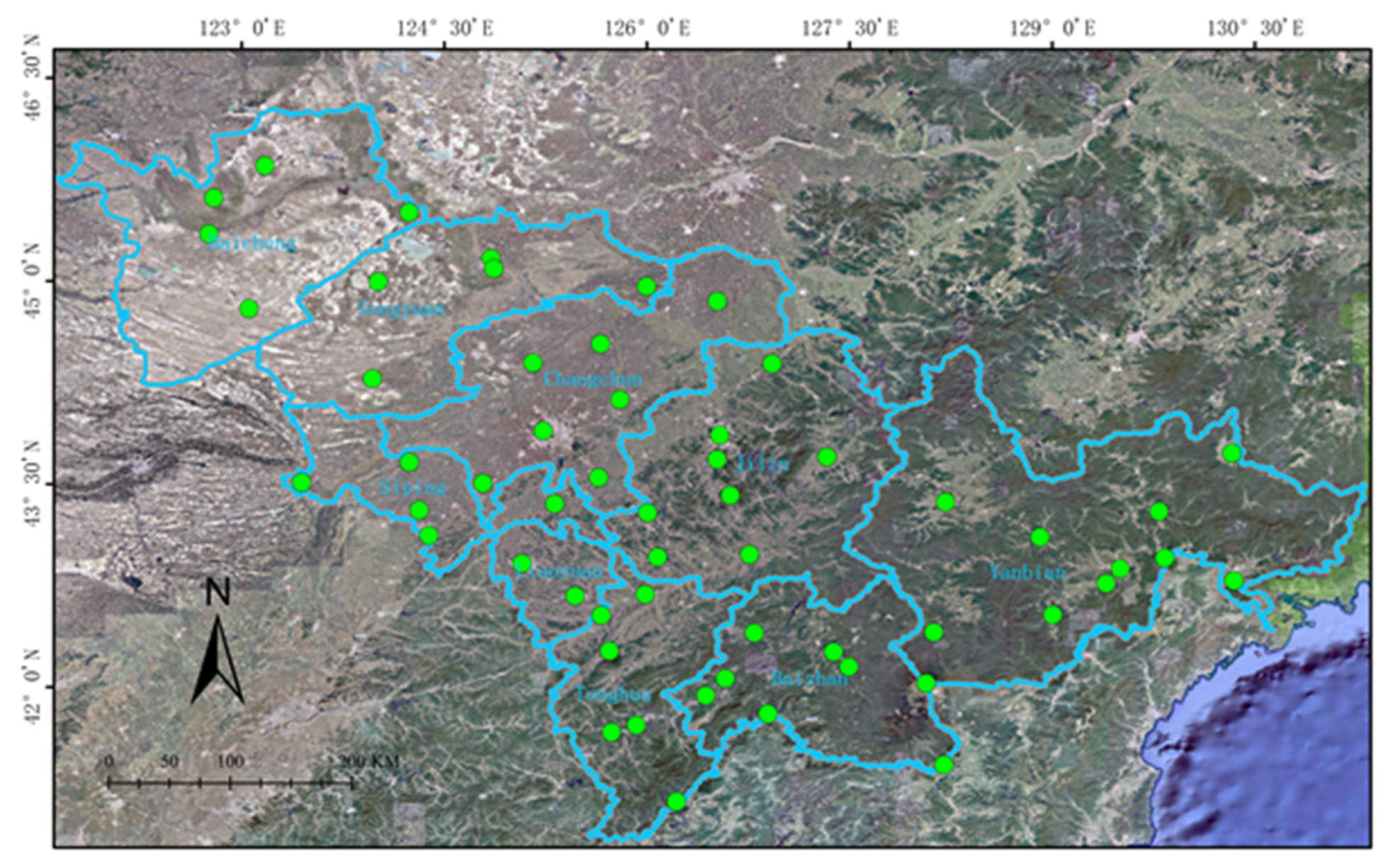
The research area of this paper is located in Jilin Province in northeastern China, and precipitation information from 56 different meteorological bureaus in cities and counties across Jilin Province was obtained.Jilin Province, located in the central part of Northeast China, is an important commodity grain base in China. 80% of annual rainfall is concentrated in summer, and the regional difference of precipitation is very obvious, which leads to natural disasters such as drought, floods and so on. The losses caused by meteorological disasters are obviously increased, threatening the lives and property of the broad masses of the people, and causing great damage to economic, social development and ecological environment. In recent years, scholars have done a lot of research on the characteristics of rainfall in Jilin Province [16–21]. The geographical locations of the meteorological stations obtained in this paper are shown in
Figure 1 below.
The geographical location of Jilin City is between 125°40' to 127°56' east longitude and 42°31' to 44°40' north latitude. It borders Yanbian Korean Autonomous Prefecture to the east, and is adjacent to Changchun and Siping to the west, Harbin in Heilongjiang Province to the north, and Baishan, Tonghua, and Liaoyuan to the south. The total area of the city is 27,120 km
2. Jilin City is located in the transition zone from the Changbai Mountains to the Songnen Plain in the central and eastern part of Jilin Province. The terrain gradually decreases from southeast to northwest. Jilin City has a temperate continental monsoon climate with distinct seasons. The study of its precipitation not only has an important impact on the activities of residents in Jilin region, but also provides important reference for global precipitation prediction work. This paper used daily precipitation data and 16 daily variables affecting precipitation, including daily average precipitation, daily wind speed, daily maximum wind speed, daily maximum wind direction, daily maximum wind direction degree, daily average dew point temperature, daily average temperature, air pressure, and relative humidity, from 56 different meteorological stations in Jilin Province provided by Jilin Meteorological Bureau for prediction. The maximum time span of the variables is the data from 1960 to 2022.
Table 1 shows the average values of each variable at each station in 2022.
The daily maximum wind direction and the daily average wind direction are non-numeric values. In the table above, the label-encoding algorithm is used to label and map each different wind direction value to a unique positive integer value, and all N positive integer values are continuous.
Table 2.
Statistics of rainfall datasets.
Table 2.
Statistics of rainfall datasets.
| index |
count |
Mean(mm) |
Standard deviation(mm) |
Precipitation(mm) |
| 25th percentile |
50th percentile |
75th percentile |
MAX |
| NWJ |
1960-2022 |
412.82 |
112.60 |
334.12 |
409.43 |
483.48 |
797.82 |
| NCJ |
1960-2022 |
566.16 |
149.33 |
452.99 |
563.54 |
673.47 |
1057.14 |
| SWJ |
1960-2022 |
510.89 |
201.78 |
434.53 |
536.64 |
632.89 |
1023.72 |
| CJ |
1960-2022 |
571.41 |
304.27 |
483.98 |
621.21 |
756.13 |
1485.33 |
| EJ |
1960-2022 |
578.53 |
168.36 |
486.75 |
587.86 |
680.25 |
1065.65 |
| SCJ |
1960-2022 |
675.46 |
155.43 |
568.55 |
644.55 |
769.25 |
1086.71 |
| SEJ |
1960-2022 |
686.27 |
349.66 |
585.69 |
729.22 |
878.96 |
1895.42 |
2.2. Data Cleaning
The dataset used in this paper contains 15 variables related to precipitation in Jilin Province from 1960 to 2022, including (i) precipitation (Pre), (ii) daily average wind speed (DAWS), (iii) daily average 10-meter wind speed (DA10WS), (iv) daily maximum wind speed (DMWS), (v) daily maximum wind speed direction (DMWSD), (vi) daily maximum wind speed direction in degrees (DMWSDD), (vii) daily extreme wind speed (DEWS), (viii) daily extreme wind speed direction (DEWSD), (ix) daily extreme wind speed direction in degrees (DEWSDD), (x) time of daily maximum wind speed (TDMWS), (xi) time of daily extreme wind speed (TDEWS), (xii) daily average dew point temperature (DADPT), (xiii) daily average air temperature (DAAT), (xiv) daily average air pressure (DAAP), and (xv) daily average relative humidity (DARH). The daily maximum wind speed direction and daily extreme wind speed direction are represented by characters indicating the direction, such as east, south, west, and north. In the data processing process, LabelEncoder is used to encode this data. The LabelEncoder method can encode multiple discrete data points and map n different discrete data points to a positive integer dataset in the range [0, n-1]. It is commonly used in deep learning for processing non-numeric variables [
22,
23].
After non-numeric encoding, missing values in the data are interpolated using cubic interpolation method [
24]. However, this method cannot effectively predict continuously missing data, causing errors in the interpolation process that will be compounded by errors from subsequent deep learning. Therefore, for each variable in the training set, continuous missing data segments are discarded if their length is more than 10% larger than the length of continuous data before and after the missing segment. For example, for the 13th meteorological station in Jilin Province, data from January 2 to April 20, 1979 is missing, and to ensure the completeness of the seasonal characteristics of precipitation, the data from this station for that year is removed from the training data. After the above processing, a total of 960,081 rows and 17 columns of complete variable data are obtained in this paper.
The obtained dataset is normalized for all dependent variables during the training process, while the independent variable of precipitation is not normalized. The normalization of dependent variables speeds up the computation of the model during operation, while not normalizing the precipitation variable allows the model to better learn the changing patterns of precipitation.
According to the Markov hypothesis, the current state only depends on the previous few states of the time series. This can be formalized as:
The joint probability distribution of an N-observation sequence in a first-order Markov chain is given by:
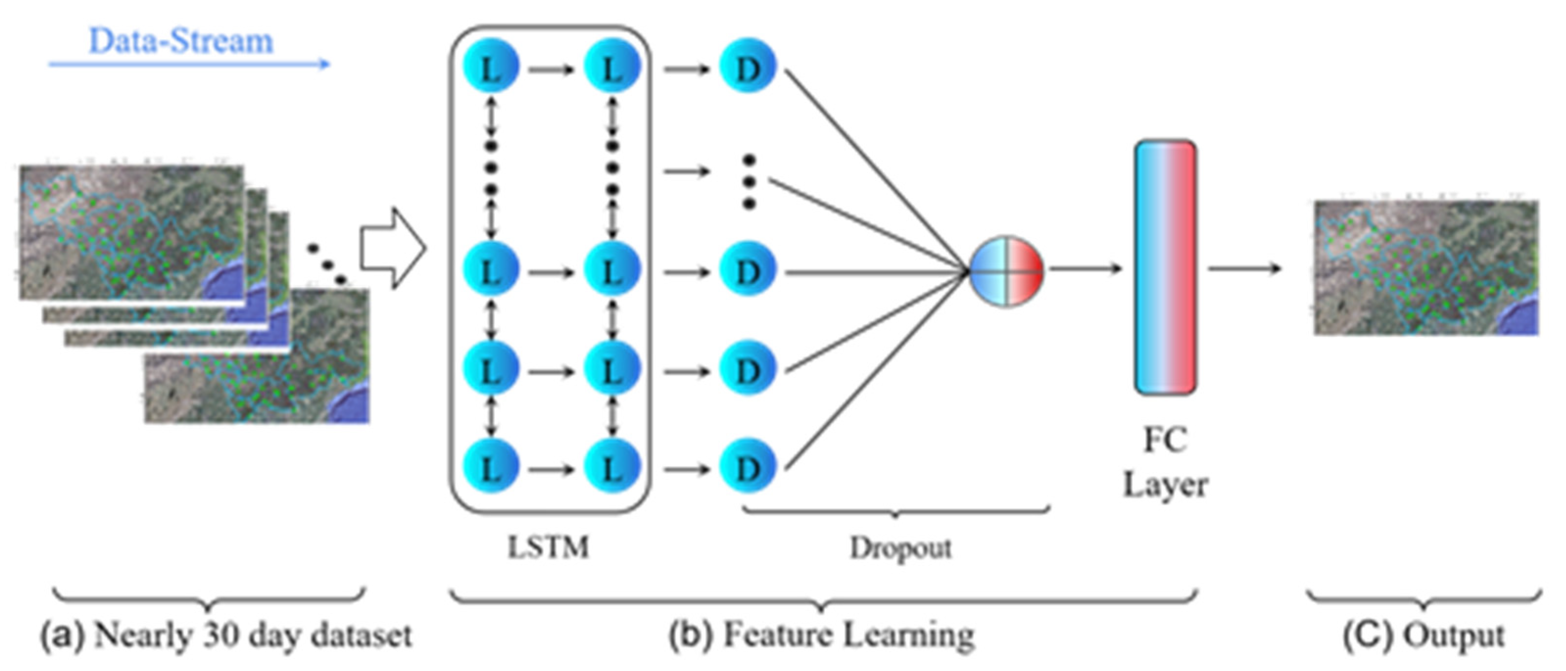
In this study, a joint dependent variable is generated by combining the previous 30 days of observations for the upcoming predicted days, which is used as the unit for precipitation prediction and training.
Figure 2.
30-day consolidated data forecasting process.
Figure 2.
30-day consolidated data forecasting process.
3. Research Method
In this paper, LSTM, Transformer, and SVR models were used for precipitation prediction, and methods such as wavelet transform, Gaussian noise, and Fourier transform were introduced to preprocess precipitation data and optimize the prediction of zero precipitation.
3.1. SVR Method
SVR is a regression model based on Support Vector Machines (SVM) that can be used to solve prediction problems with continuous target variables. Unlike traditional regression models, SVR maps input data to a high-dimensional space using a kernel function, and finds the optimal hyperplane in that space to fit the data.
The core idea of SVR is to transform the dataset into a high-dimensional space, making the data linearly separable or approximately linearly separable in the new space. By using a kernel function, SVR effectively avoids computation problems in high-dimensional space, enabling efficient regression analysis.
Specifically, the SVR model determines the optimal regression function by minimizing the error between the training data and the model. During training, the SVR model first maps the training data to a high-dimensional space, and then uses support vectors to determine the optimal hyperplane. This hyperplane is the optimal solution that minimizes the prediction error of the model while maintaining low complexity.
where y is the target variable, x is the independent variable, f(x) is the regression function, and ϵ is the error term.
SVR typically uses the least squares method to solve the regression equation in order to simplify the problem. Assuming there are N training samples(xi ,yi), the goal of the least squares method is to minimize the sum of squared residuals.
where H is the Hilbert space with the kernel function, and C is a regularization parameter.
To transform nonlinear problems into linear ones, SVR employs kernel functions to map input data to a high-dimensional space. The kernel function typically takes the form of:
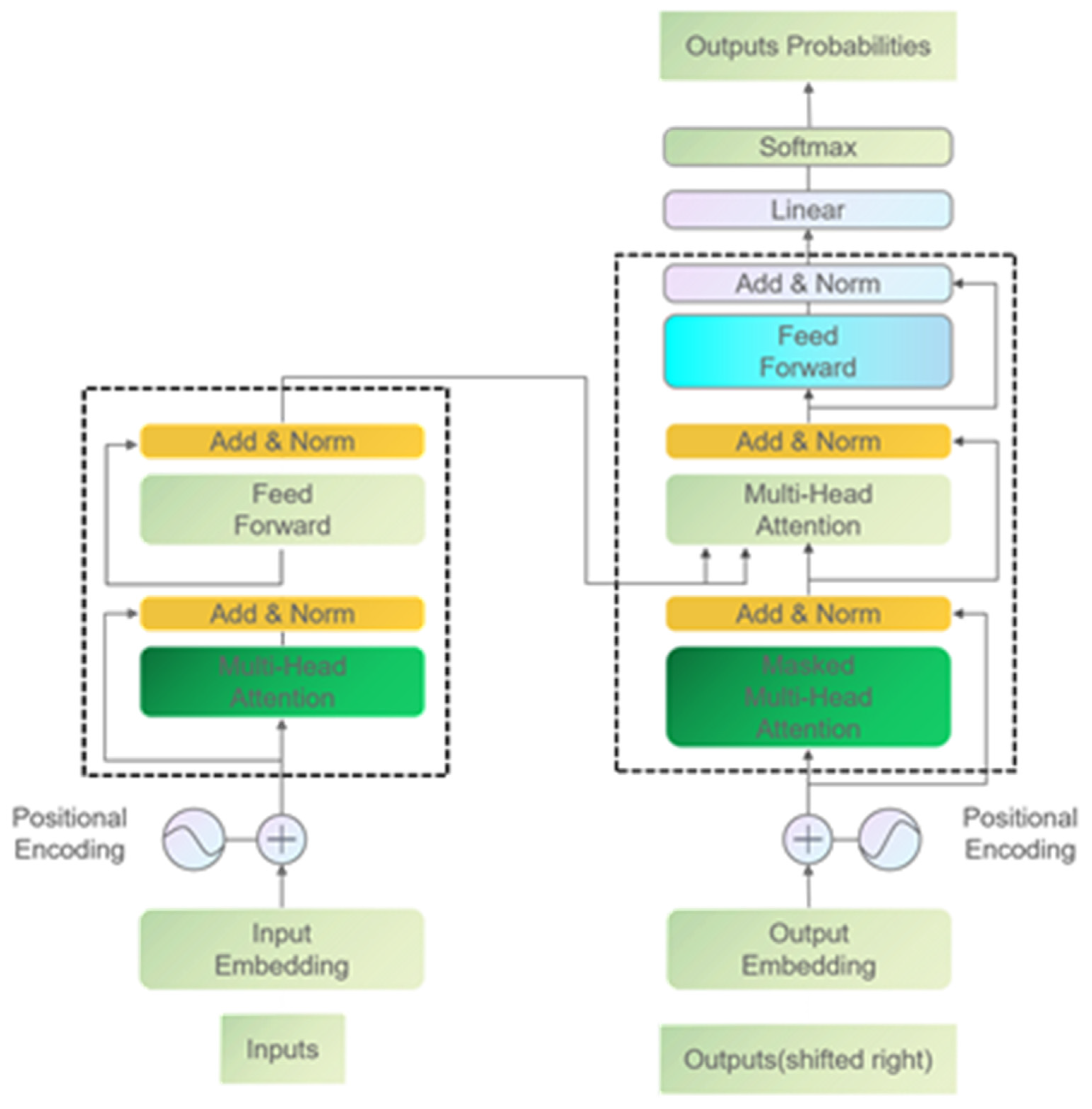
3.2. Transformer Method
The Transformer is a sequence-to-sequence (seq2seq) model based on attention mechanism, proposed by Google in 2017 [
30], aimed at addressing the shortcomings of traditional recurrent neural network (RNN) and LSTM models. The Transformer model is widely used in natural language processing tasks such as machine translation, text generation, and speech recognition.
The Transformer model adopts an Encoder-Decoder architecture, where the input sequence is processed by multiple layers of encoders, and the output sequence is generated through the decoder. Each encoder and decoder contains two modules: multi-head attention mechanism and feed-forward neural network. The attention mechanism is used to extract key information from the input sequence, while the feed-forward neural network is used to process and transform the extracted information.
The attention mechanism in the Transformer model is based on self-attention, which can automatically adjust the weights of different positions according to the context relationships in the input sequence, so as to extract key information. The formula for computing self-attention is as follows:
The Q, K, and V in this formula are the query, key, and value vectors of the input sequence, respectively, with dk representing the dimensionality of the vectors. This formula can be seen as calculating the similarity between the query vector Q and all key vectors K, normalizing the results, and then multiplying the normalized result with the value vector V to obtain the output.
In the Transformer model, there are not only single attention mechanisms but also multi-head attention mechanisms. Multi-head attention mechanisms can simultaneously extract different aspects of the input sequence, thereby improving the expressive power and generalization ability of the model.
In summary, the Transformer model effectively solves the problems of traditional recurrent neural network models by introducing innovations such as self-attention and multi-head attention mechanisms, and has become one of the popular models in the field of time-series.
Figure 3.
LSTM architecture.
Figure 3.
LSTM architecture.
3.3. LSTM Method
The LSTM model [
25] is a type of deep learning model used to process data with a time-series structure, such as weather forecasting, speech recognition, and natural language processing. LSTM is a type of Recurrent Neural Network (RNN) designed to solve the problems of vanishing and exploding gradients in traditional RNN models.
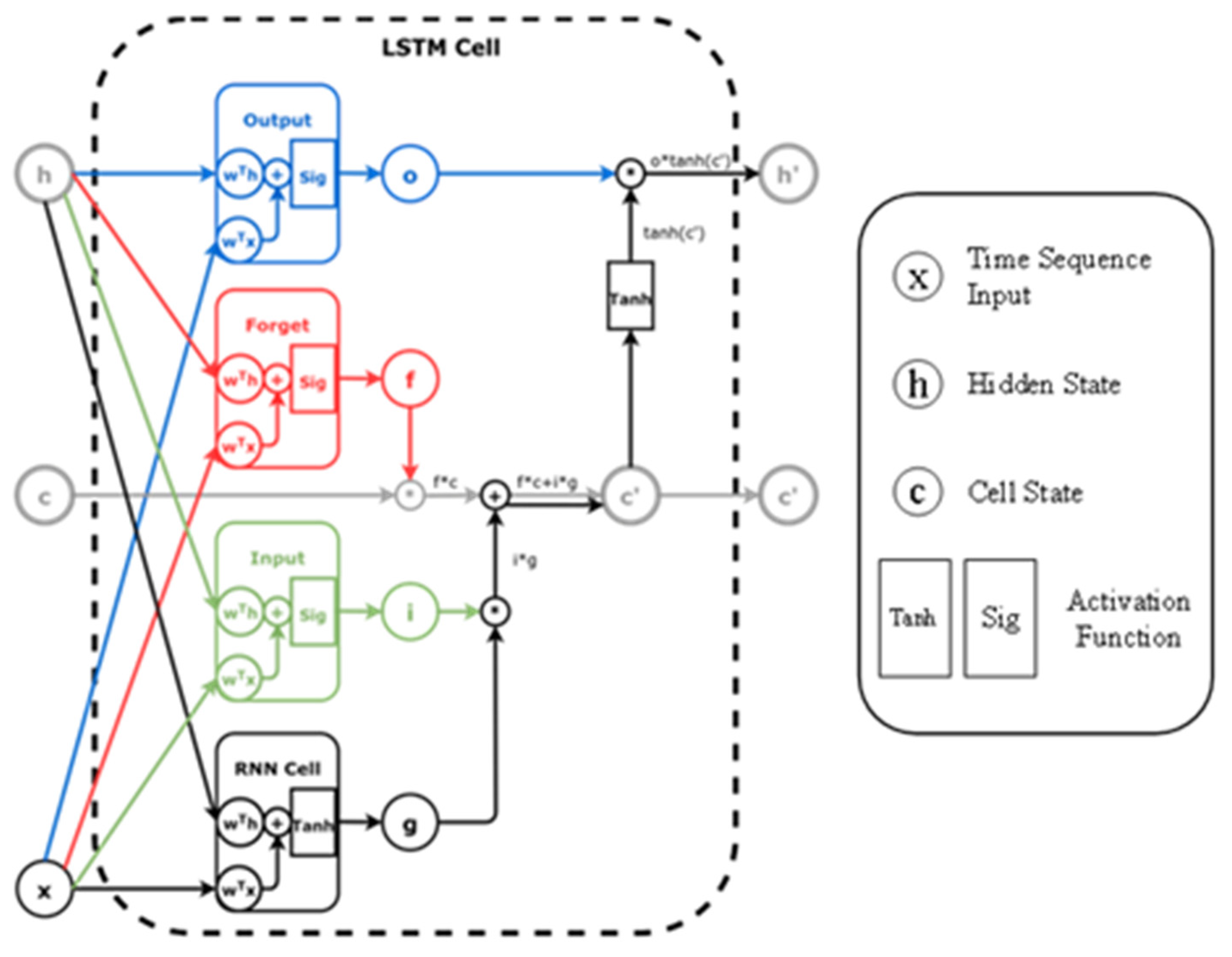
Unlike traditional RNNs, each neuron in the LSTM model has three gates (a type of neural network structure used to control the flow of information in and out), namely the input gate, forget gate, and output gate. These gates allow the network to selectively remember and forget information, enabling the network to better handle long sequential data.
Specifically, the LSTM model consists of an input layer, an output layer, and one or more LSTM layers. In the input layer, the LSTM model receives time-series data as input and feeds it into the LSTM layer. In the LSTM layer, LSTM units generate the current hidden state based on the current input and the previous hidden state, and pass it to the next time step. This way, the LSTM model can capture long-term dependencies in the data and pass this information to subsequent time steps.
Figure 4.
LSTM architecture.
Figure 4.
LSTM architecture.
In the above figure, sig represents the Sigmoid function:
The implementation of the forget gate can be represented as:
The forget gate uses Sigmoid activation to decide what information should be forgotten or retained. It calculates the value of C based on Ht-1 and Xt, where C ranges from 0 to 1. A value of 0 indicates complete forgetfulness, while a value of 1 means complete retention of information.
The implementation of the input gate can be represented as:
At this step, again, a Sigmoid is used to determine whether the data should be updated. A tanh layer is then used to create a vector that will be combined with the Sigmoid output to update the cell state.
The updating process of the cell state is as follows:
The implementation of the output gate can be represented as:
The content output by the final output layer is based on the Cell State. First, the content of the Cell State is compressed to the range of [-1, 1] by the tanh function, and then multiplied with the output of the Sigmoid function to obtain the final output. During the training process, the LSTM model uses backpropagation algorithm to update parameters to minimize the loss function. Through continuous training, the LSTM model can gradually learn the patterns in the data and predict future results given input data.
In the Jilin region precipitation prediction task, the LSTM model can receive historical precipitation data as input and predict the precipitation in the future. With appropriate tuning and training, the LSTM model can achieve good prediction performance.
In this paper employs two commonly used types of LSTM structures, namely Vanilla LSTM [
26,
27] and Stacked LSTM [
34,
35]. Vanilla LSTM is the traditional LSTM model structure, while Stacked LSTM has additional hidden layers, making the model deeper and more accurately described as a deep learning technique. The depth of neural networks enables their success in challenging prediction problems. Additional hidden layers can be added to a multilayer perceptron neural network, making it deeper. The additional hidden layers are understood as recombining learned representations from previous layers, and creating new representations at higher levels of abstraction [
28]. For example, from linear to shape to object. A large enough single hidden layer multilayer perceptron can be used to approximate most functions. Increasing the depth of the network provides an alternative solution that requires fewer neurons and faster training. Finally, increasing depth is a representative optimization technique.
Figure 5.
Vanilla LSTM and Stacked LSTM.
Figure 5.
Vanilla LSTM and Stacked LSTM.
3. Experiments and Results
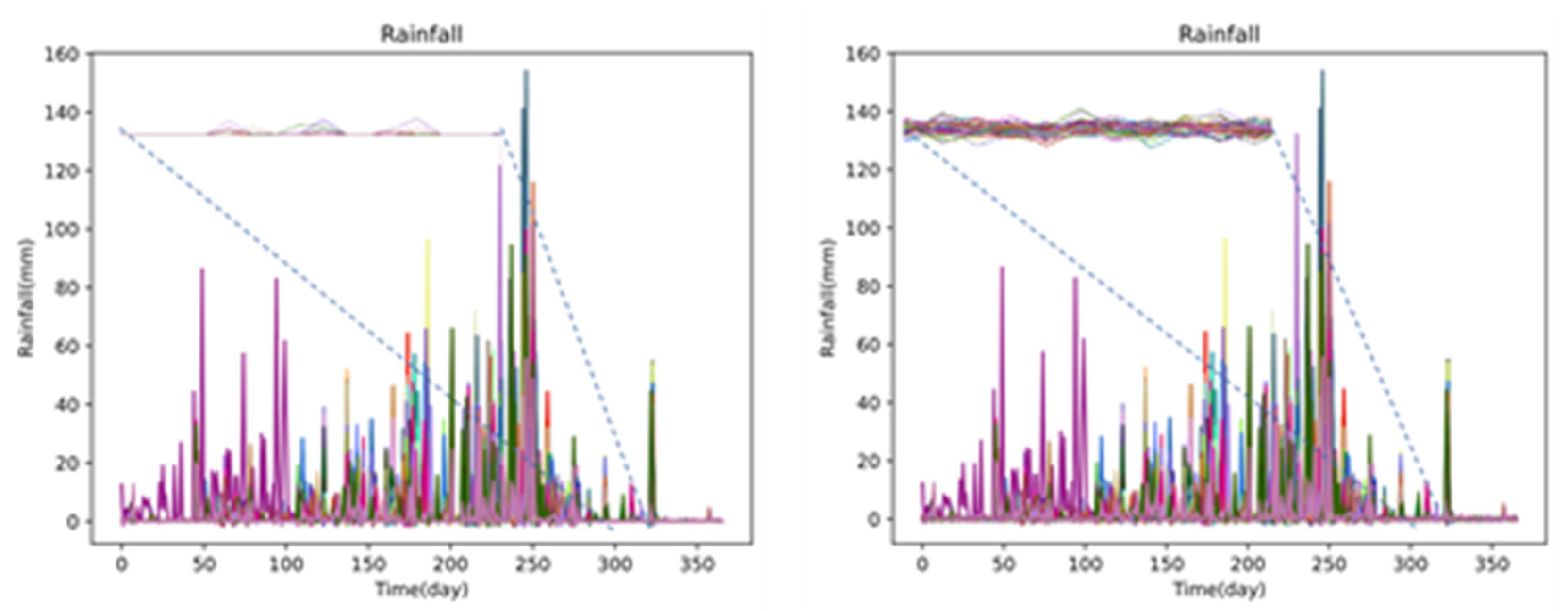
In this paper, the dataset of each station was divided, with precipitation data from 1960 to 2020 used as the training set and precipitation data from 2021 used as the test set. To avoid specific optimizations for the test set during model optimization, which may reduce the robustness of the model, the final result was evaluated using the latest precipitation data from 2022 as the measure. Additionally, based on the precipitation data from 56 meteorological stations in 2020, there were a total of 20,252 days with valid daily precipitation, among which 12,072 days had zero precipitation, accounting for approximately 59.61%. A large amount of identical zero precipitation data leads to poor performance of the deep learning model in predicting zero precipitation. Therefore, this article used the method of adding Gaussian noise to the data to add noise to the data.Rainfall with and withour added noi seis shown in the figure below:
Figure 6.
Rainfall with and without added Gaussian niose.
Figure 6.
Rainfall with and without added Gaussian niose.
Gaussian noise, also known as normal distribution noise, is a commonly used random noise model. According to the central limit theorem, when a random variable is the sum of many independent random variables with the same distribution, the random variable will approximate a normal distribution. Therefore, adding random noise that follows a Gaussian distribution to data can simulate many noise sources in the real world. Adding Gaussian noise to data is a commonly used data augmentation technique in deep learning. It can effectively help the model learn more data features, increase the model's generalization ability, and thus improve the model's accuracy. Specifically, the formula for adding Gaussian noise to data x is as follows:
The epsilon (ϵ) is a random number that follows a Gaussian distribution with a mean of 0 and a standard deviation of ϵ. Typically, its value is chosen based on the specific situation, ranging from 0.01 to 0.1. In this article, it is set to 0.1. Its probability distribution function can be represented as:
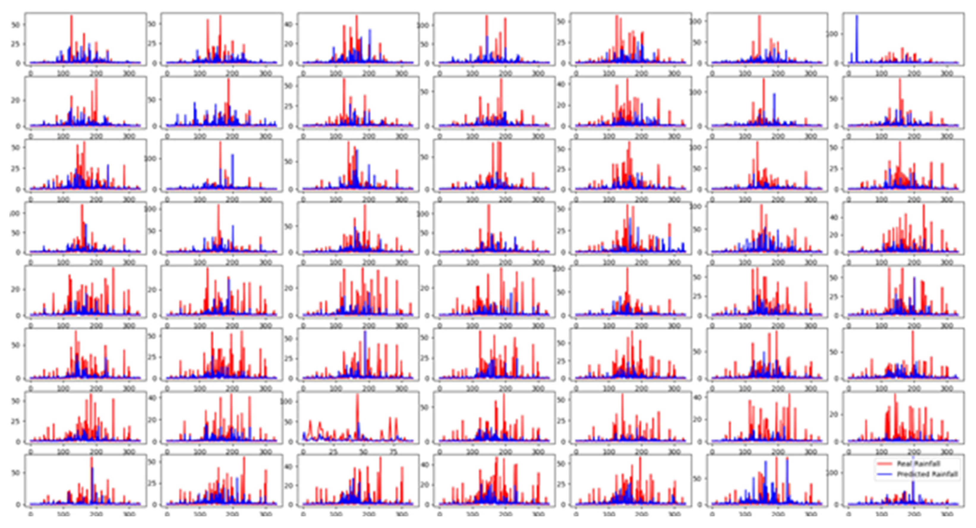
After comparing the three models mentioned above, this article found that using the Stacked-LSTM model for predicting precipitation had the best results. Its parameters included a loss function of MSE (Mean Square Error), an optimizer of Adam (adaptive moment estimation), a batch size of 1, and 250 epochs. The specific predicted values and actual values are shown in the following figure:
Figure 7.
The precipitation prediction of 56 meteorological stations for 2022.
Figure 7.
The precipitation prediction of 56 meteorological stations for 2022.
The root mean square error (RMSE) is a commonly used metric for measuring the difference between the predicted values and the true values in regression models. It helps evaluate the accuracy of the model. The RMSE is calculated by taking the average of the squared differences between the predicted and true values, and then taking the square root. The mathematical formula for RMSE is:
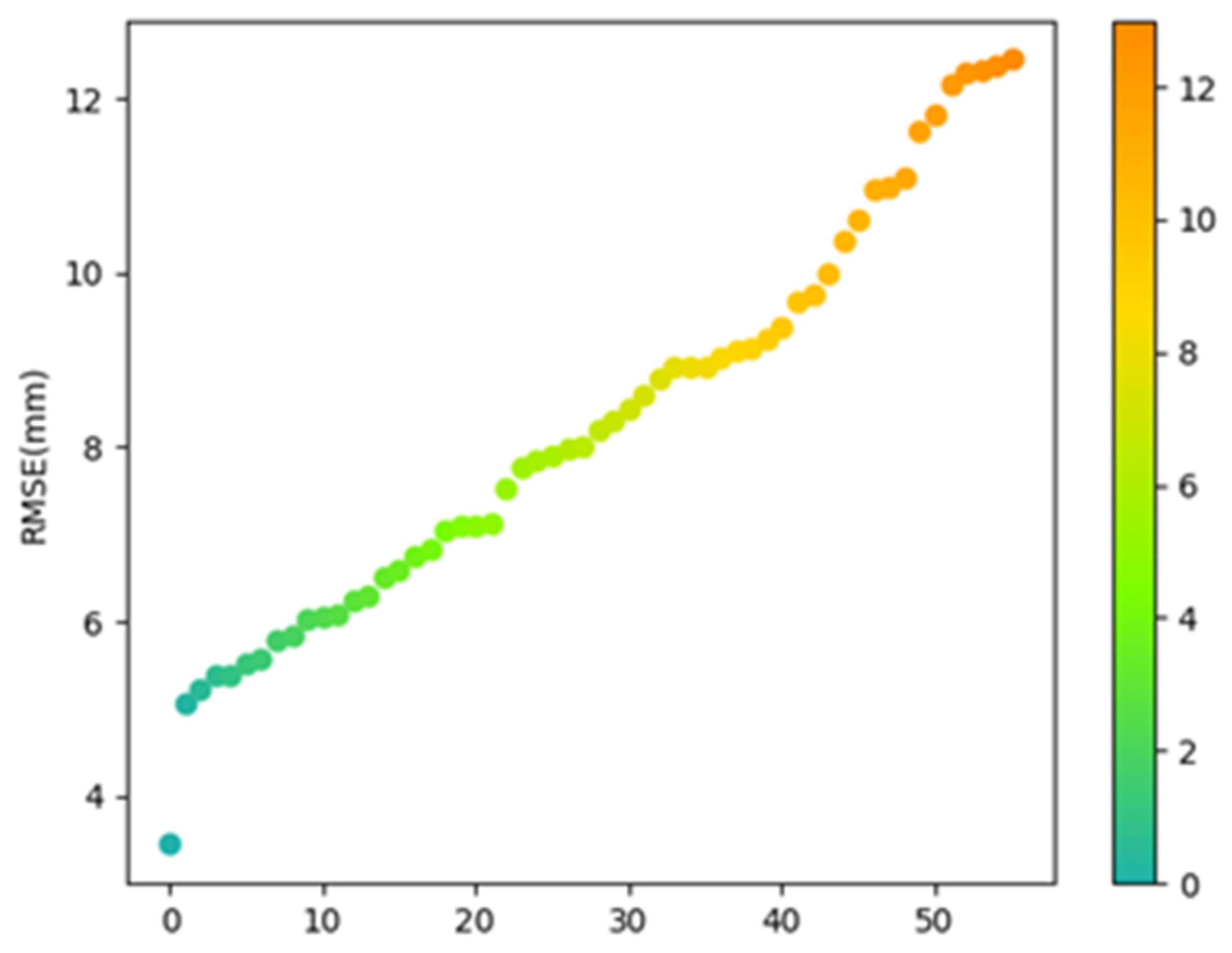
The RMSE (Root Mean Square Error) is a common metric to measure the difference between the predicted and true values in regression models, and it can help us evaluate the accuracy of the model. A smaller RMSE indicates a smaller gap between the predicted and true values, and a better predictive capability of the model. In this article, the RMSE for the best model's prediction on 56 meteorological stations is shown in the figure below:
Figure 8.
The RMSE of 56 meteorological stations.
Figure 8.
The RMSE of 56 meteorological stations.
4. Conclusions
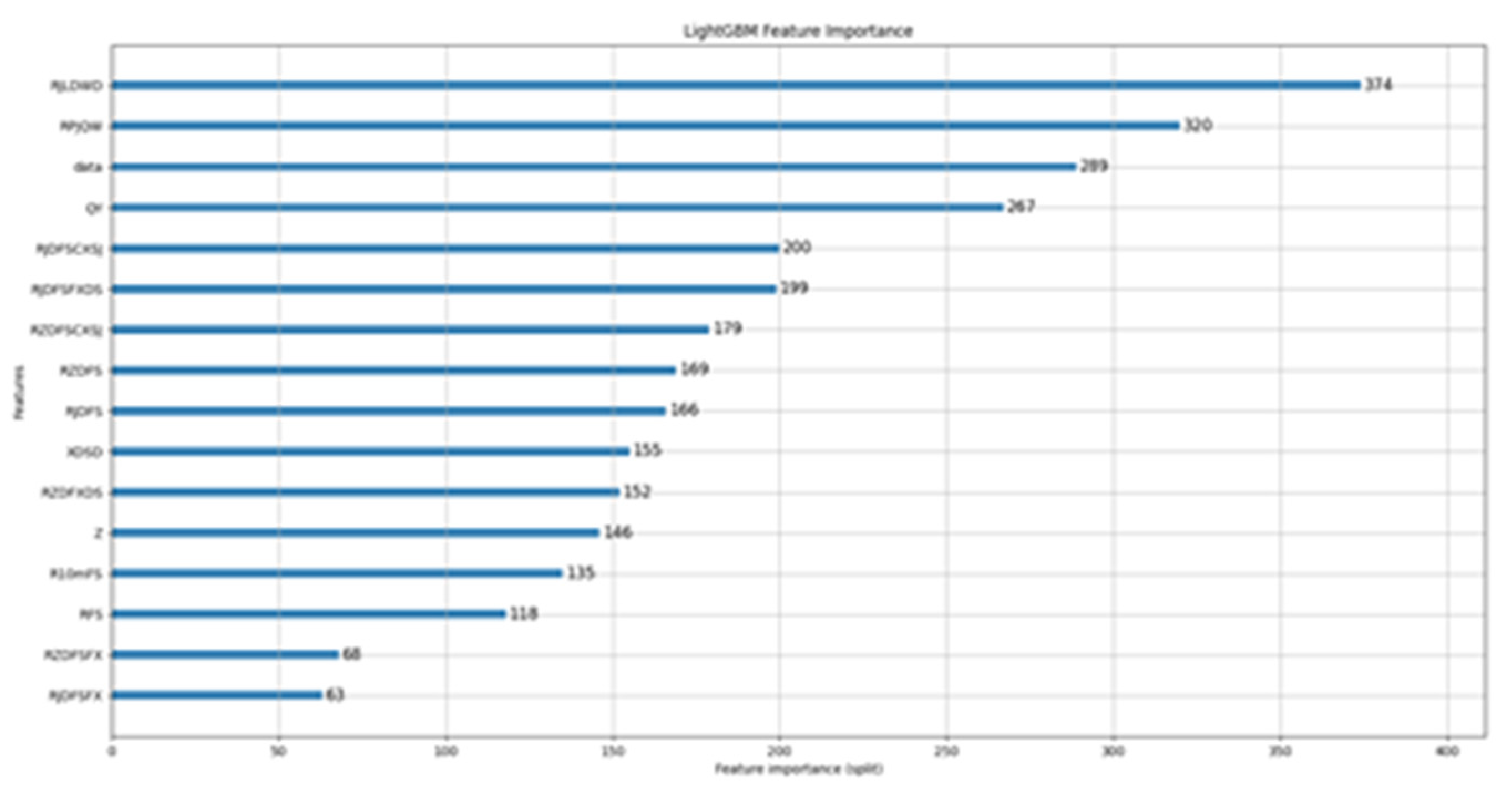
This paper sused three different models (Stacked-LSTM, Transformer, SVR) to predict precipitation in 56 meteorological stations in Jilin Province, and improved the robustness of the models by adding Gaussian noise to the data. The experimental results showed that the Stacked-LSTM model performed the best in this task, achieving high prediction accuracy and stability. For the 16 different variables used in this article, the article conducted attribution analysis on the variables using the LightGBM [31–33] algorithm, and the conclusions are as follows:
Figure 9.
Variable attribution analysis.
Figure 9.
Variable attribution analysis.
This paper explores the use of deep learning models, specifically Stacked-LSTM, Transformer, and SVR, for predicting precipitation in 56 weather stations in Jilin province. Gaussian noise is added to the data to improve the robustness of the models. The results show that Stacked-LSTM performs the best, achieving high prediction accuracy and stability.
The importance of different variables in the prediction process was analyzed using the LightGBM algorithm for variable attribution analysis. The findings show that the importance of different variables is consistent with traditional meteorological experience and theory. The most influential factors include daily dew point temperature, daily air temperature, previous precipitation, and air pressure. Dew point temperature and air temperature ensure the generation of rainwater in the atmosphere and are crucial factors for predicting the likelihood of precipitation. Previous precipitation provides important trends and directions for predicting precipitation, while air pressure affects whether water vapor in the air will rise to a sufficient height to generate precipitation.
Furthermore, the article provides detailed information on the training process, including data preprocessing and model parameter settings, which can be useful for future precipitation prediction tasks. Additionally, the article finds that adding Gaussian noise can improve the model's generalization ability for datasets with many zero precipitation days, leading to better prediction results.
In conclusion, this article verifies the performance of different models in precipitation prediction tasks and provides a reference for related research fields. The use of more advanced data preprocessing techniques and model optimization methods can further improve model performance and applicability, promoting the development of meteorological prediction and applications in the future.
Acknowledgments
This work was supported by Guangxi science and technology base, and talent project (2020AC19134).
References
- Nourani, V.; Alami, M.T.; Aminfar, M.H. A combined neural-wavelet model for prediction of Ligvanchai watershed precipitation. Eng. Appl. Artif. Intell. 2009, 22, 466–472. [Google Scholar] [CrossRef]
- Xu, D.; Zhang, Q.; Ding, Y.; Zhang, D. Application of a hybrid ARIMA-LSTM model based on the SPEI for drought forecasting. Environ. Sci. Pollut. Res. 2021, 29, 4128–4144. [Google Scholar] [CrossRef]
- Xu, D.; Zhang, Q.; et al. Application of a Hybrid ARIMA–SVR Model Based on the SPI for the Forecast of Drought—A Case Study in Henan Province, China. Journal of Applied Meteorology and Climatology 2022, 59, 1239–1259. [Google Scholar] [CrossRef]
- Xiang, Y.; Gou, L.; He, L.; Xia, S.; Wang, W. A SVR–ANN combined model based on ensemble EMD for rainfall prediction. Appl. Soft Comput. 2018, 73, 874–883. [Google Scholar] [CrossRef]
- Kumar, R.; Singh, M.P.; Roy, B.; Shahid, A.H. A Comparative Assessment of Metaheuristic Optimized Extreme Learning Machine and Deep Neural Network in Multi-Step-Ahead Long-term Rainfall Prediction for All-Indian Regions. Water Resour. Manag. 2021, 35, 1927–1960. [Google Scholar] [CrossRef]
- Kumar, D.; Singh, A.; Samui, P.; Jha, R.K. Forecasting monthly precipitation using sequential modelling. Hydrol. Sci. J. 2019, 64, 690–700. [Google Scholar] [CrossRef]
- Xu, D.; Ding, Y.; Liu, H.; Zhang, Q.; Zhang, D. Applicability of a CEEMD–ARIMA Combined Model for Drought Forecasting: A Case Study in the Ningxia Hui Autonomous Region. Atmosphere 2022, 13, 1109. [Google Scholar] [CrossRef]
- Poornima, S.; Pushpalatha, M. Drought prediction based on SPI and SPEI with varying timescales using LSTM recurrent neural network. Soft Comput. 2019, 23, 8399–8412. [Google Scholar] [CrossRef]
- Ziegel, E.R.; Box, G.E.P.; Jenkins, G.M.; et al. Time Series Analysis, Forecasting, and Control. Journal of Time 1976, 31, 238–242. [Google Scholar] [CrossRef]
- Pai, P.-F.; Hong, W.-C. A recurrent support vector regression model in rainfall forecasting. Hydrol. Process. 2006, 21, 819–827. [Google Scholar] [CrossRef]
- Chiang, S.; Chang, C.H.; Chen, W.B. Comparison of Rainfall-Runoff Simulation between Support Vector Regression and HEC-HMS for a Rural Watershed in Taiwan. Water 2022, 14, 191. [Google Scholar] [CrossRef]
- Liu, H.-L.; Bao, A.-M.; Chen, X.; Wang, L.; Pan, X.-L. Response analysis of rainfall-runoff processes using wavelet transform: a case study of the alpine meadow belt. Hydrol. Process. 2011, 25, 2179–2187. [Google Scholar] [CrossRef]
- Unnikrishnan, P.; Jothiprakash, V. Hybrid SSA-ARIMA-ANN Model for Forecasting Daily Rainfall. Water Resour. Manag. 2020, 34, 3609–3623. [Google Scholar] [CrossRef]
- Xiao, W.W.; Luan, W.J. The Application of Wavelet Neural Networks on Rainfall Forecast. Applied Mechanics and Materials 2013, 263–266, 3370–3373. [Google Scholar] [CrossRef]
- Chen, S.; Xu, X.; Zhang, Y.; Shao, D.; Zhang, S.; Zeng, M. Two-stream convolutional LSTM for precipitation nowcasting. Neural Comput. Appl. 2022, 34, 13281–13290. [Google Scholar] [CrossRef]
- Liu, B. Spatial Distribution and Periodicity Analysis of Annual Precipitation in Jilin Province. Water Resources and Power 2018. [Google Scholar]
- Li, Y.F.; Xu, S.Q.; Zhang, T.; et al. Regional characteristics of interdecadal and interannual variations of summer precipitation in Jilin Province. Meteorol. Disaster Prev 2018, 25, 38–43. [Google Scholar]
- Li, M.; Wu, Z.F.; Meng, X.J.; et al. Temporal-spatial distribution of precipitation over Jilin Province during 1958~2007. J. Northeast Normal Univ. (Nat. Sci. Ed.) 2010, 42, 146–151. [Google Scholar]
- Sun, Y.; Yang, Z.C.; Yun, T.; et al. Weather characteristics of short-term heavy rainfall and large-scale environmental conditions in Jilin Province. Meteorol. Disaster Prev 2015, 229, 12–33. [Google Scholar]
- Li, M.; Wu, Z.F.; Meng, X.J.; et al. Temporal-spatial distribution of precipitation over Jilin Province during 1958~2007. J. Northeast Normal Univ. (Nat. Sci. Ed.) 2010, 42, 146–151. [Google Scholar]
- Lin, M.K.; Wei, N.; Xie, J.C.; Lu, K.M. Study on multi-time scale variation rule of rainfall during flood season in Jilin Province in recent 65 years. IOP Conf. Series: Earth Environ. Sci. 2019, 344, 012143. [Google Scholar] [CrossRef]
- G, T.R.; Bhattacharya, S.; Maddikunta, P.K.R.; Hakak, S.; Khan, W.Z.; Bashir, A.K.; Jolfaei, A.; Tariq, U. Antlion re-sampling based deep neural network model for classification of imbalanced multimodal stroke dataset. Multimedia Tools Appl. 2020, 81, 41429–41453. [Google Scholar] [CrossRef]
- Senan, E.M.; Al-Adhaileh, M.H.; Alsaade, F.W.; Aldhyani, T.H.H.; Alqarni, A.A.; Alsharif, N.; Uddin, M.I.; Alahmadi, A.H.; E Jadhav, M.; Alzahrani, M.Y. Diagnosis of Chronic Kidney Disease Using Effective Classification Algorithms and Recursive Feature Elimination Techniques. J. Health Eng. 2021, 2021, 2040–2295. [Google Scholar] [CrossRef] [PubMed]
- Shirman, L.; Séquin, C. Procedural interpolation with curvature-continuous cubic splines. Comput. Des. 1992, 24, 278–286. [Google Scholar] [CrossRef]
- Hochreiter, S.; Schmidhuber, J. Long Short-Term Memory. Neural Computation 1997, 9, 1735–1780. [Google Scholar] [CrossRef] [PubMed]
- Graves, A.; Schmidhuber, J. Framewise phoneme classification with bidirectional LSTM and other neural network architectures. Neural Netw. 2005, 18, 602–610. [Google Scholar] [CrossRef] [PubMed]
- Greff, K.; Srivastava, R.K.; Koutník, J.; Steunebrink, B.R.; Schmidhuber, J. LSTM: A Search Space Odyssey. IEEE Trans. Neural Netw. Learn. Syst. 2017, 28, 2222–2232. [Google Scholar] [CrossRef]
- Hermans, M.; Schrauwen, B. Training and analysing deep recurrent neural networks. Advances in neural information processing systems 2013. [Google Scholar]
- Graves, Alex; Mohamed, Abdel-rahman; Hinton, Geoffrey (2013)., Speech and Signal Processing - Speech recognition with deep recurrent neural networks. PP 6645–6649. [CrossRef]
- Vaswani A, Shazeer N, Parmar N, et al. Attention Is All You Need. arXiv, 2017.
- Liang, J.; Bu, Y.; Tan, K.; Pan, J.; Yi, Z.; Kong, X.; Fan, Z. Estimation of Stellar Atmospheric Parameters with Light Gradient Boosting Machine Algorithm and Principal Component Analysis. Astron. J. 2022, 163. [Google Scholar] [CrossRef]
- Cui, Z.; Qing, X.; Chai, H.; Yang, S.; Zhu, Y.; Wang, F. Real-time rainfall-runoff prediction using light gradient boosting machine coupled with singular spectrum analysis. J. Hydrol. 2021, 603, 127124. [Google Scholar] [CrossRef]
- Liang, Y.; Wu, J.; Wang, W.; Cao, Y.; Zhong, B.; Chen, Z.; Li, Z. Product Marketing Prediction based on XGboost and LightGBM Algorithm[C]//0[2023-07-01]. [CrossRef]
- Zeng, C.; Ma, C.; Wang, K.; et al. Parking Occupancy Prediction Method Based on Multi Factors and Stacked GRU-LSTM. IEEE Access 2022, 10, 47361–47370. [Google Scholar] [CrossRef]
- Hermans M, Schrauwen B. Training and analysing deep recurrent neural networks[J]. Advances in neural information processing systems, 2013.
- Cheng X, Rao Z, Chen Y, et al. Explaining Knowledge Distillation by Quantifying the Knowledge[J]2020 IEEE CVF Conference on Computer Vision and Pattern Recognition (CVPR). IEEE, 2020.
Short Biography of Authors
 |
Yibo Zhang received the master’s degree in Cartography and Geographical Information System from Jilin University, China. He is currently a lecturer with Jilin Provincial Meteorological Information and Network Center, China. He has published more than 10 papers in journals, including the World Geology, Meteorological Disaster Prevention, and others. His current research interests include machine learning, deep learning, GIS, data analysis, and meta-learning and their applications to address geological and Meteorological problems. |
 |
Chengcheng Wang received the master’s degree in software engineering from Jilin University, China. She is currently an Associate Professor with Jilin Provincial Meteorological Information and Network Center, China. She has published 6 papers in journals, including the Agriculture of Jilin, Meteorological Disaster Prevention, Modern Agricultural Science and Technology, Journal of Sichuan Normal University (Natural Science), and others. Her current research interests include machine learning and deep learning and their applications to address Meteorological problems. |
 |
Pengcheng Wang is Graduate student in progress from East China Normal University, China. He has published 5 papers in journals, including the Computer & Telecommunication, and others. His current research interests include machine learning, and deep learning, and their applications to address geological problems. |
 |
Lu Zhang received the Master degree in electronic information engineering from Southwest Jiaotong University, China. Her current research interests include machine learning, math-ematics, and their application in solving geological problems and the medical field. |
 |
Qingbo Yu is currently pursuing a master's degree in agricultural extension and graduated from Chengdu University of Information Technology. He is a senior engineer qualification at the Jilin Provincial Meteorological Information Network Center, mainly engaged in research in meteorological data processing and analysis, deep learning. More than 10 papers have been published in journals, and their data processing and analysis, as well as deep learning research achievements, are mainly applied in the field of meteorology. |
 |
Hui Xu graduated from Nanjing University with a master's degree in meteorology, she is an associate senior engineer, and she has had 8 papers accepted by national journals. Her main research interests are climate change, climate data analysis and processing. |
 |
Maofa Wang received the Ph.D. degree in geo-information engineering from Jilin University, China. He is currently a Professor with the School of Computer and Information Security, Guilin University of Electronic Technology, China. He has published more than 20 papers in international journals and conference proceedings, including the Journal of Seismology, Computers & Geosciences, and others. His current research interests include machine learning, deep learning, and meta-learning and their applications to address geological problems. |
|
Disclaimer/Publisher’s Note: The statements, opinions and data contained in all publications are solely those of the individual author(s) and contributor(s) and not of MDPI and/or the editor(s). MDPI and/or the editor(s) disclaim responsibility for any injury to people or property resulting from any ideas, methods, instructions or products referred to in the content. |
© 2023 by the authors. Licensee MDPI, Basel, Switzerland. This article is an open access article distributed under the terms and conditions of the Creative Commons Attribution (CC BY) license (http://creativecommons.org/licenses/by/4.0/).
