
Submitted:
21 August 2023
Posted:
22 August 2023
You are already at the latest version
Abstract
Knowledge of permafrost’s ice and unfrozen water content is critical for predicting the permafrost behavior during ice–water–ice transition. This is especially relevant when ice and permafrost are melting in many regions under the influence of global warming. It is well-known that only a part of the formation's pore water turns into ice at 0 ^oC. After the further lowering the temperature, the water phase transition continues, but at gradually decreasing rates. Thus, the porous space is filled with ice and unfrozen water. The laboratory data show that frozen formations' mechanical, thermal, and rheological properties strongly depend on the moisture content. Hence, porosity and temperature are essential parameters of permafrost. In this paper, it is shown how, and by combining research in three fields: (1) geophysical exploration, (2) numerical modeling, and (3) temperature logging, it is possible to estimate in-situ the porosity of permafrost. To demonstrate the procedure, five examples of numerical modeling (where all input parameters are specified) are given. This investigation is the first attempt to analyze the permafrost’s porosity in situ quantitively.
Keywords:
permafrost
; porosity
; refreezing time
; shut-in temperature
2 Azerbaijan State Oil and Industry University, 20 Azadlig Ave., Baku AZ1010, Azerbaijan
1. Introduction
It is well-known that only a part of the formation’s pore water turns into ice at 0 oC. With the additional lowering of the temperature, the phase transition of the water continues, however, at gradually decreasing rates. The quantity of unfrozen water is practically independent of the total moisture content for soil with the concrete physical-chemical parameters (Tsytovich, 1975). Frozen soil is the matter in which stresses and strains arise under the influence of an external load. These forces are not constant but vary with time. It gives rise to the relaxation of stresses and creeps (i.e., increased strains over time). These complex physical-chemical processes are called rheological ones. The vigorous development of the rheological processes in frozen soils is caused by the peculiarities of their internal relationships in which ice plays a significant role. Numerous laboratory experiments show that frozen formations’ mechanical, thermal, and rheological properties strongly depend on the moisture content. Hence, porosity and temperature are essential parameters of permafrost. It is known that the electric resistivities of frozen sediments are affected by the freezing-thawing transition to a greater extent than the seismic velocities. In the same interval of temperatures, seismic velocities may increase by 2 to 10 times in transition to a frozen condition, whereas the electrical resistivity may increase by 3·10 – 3·102 times (Hnatiuk and Randall, 1977; Dobinski, 2011; Eppelbaum, 2021). The position of the interface of the thawing-freezing transition can be determined with the application of the surface electric resistivity method and sonic logs in wells. For instance, the transition from higher resistivity and velocity values to lower ones can be considered the thawing radius's position. Thus, the position of the radius of thawing (because of well drilling or production) can be estimated by using different geophysical exploration methods. A method of estimating the refreezing time surrounding the wellbore thawed (during drilling) formations was suggested by Kutasov and Eppelbaum (2017, 2018). Only three temperature logs taken after the freezeback are completed and are needed to apply this method. The conducted numerical modeling indicates that the dimensionless time of refreezing can be expressed as a function of two dimensionless parameters: radius of thawing and latent heat density (Kutasov, 2006; Eppelbaum and Kutasov, 2018). From the last parameter, the porosity of formations can be estimated.
The only objective of this study is to offer a possible way to estimate permafrost's porosity in situ. This study is the first effort to determine this parameter in natural conditions. This parameter in situ estimation is of special importance when the permafrost parameters are constantly changing under the influence of global warming. To demonstrate the possibility of the new approach applicability of this new method, five cases of numerical modeling are presented.
2. Time of freezeback
Since deep wells drilling in permafrost areas usually use warm mud, a certain unknown degree of the formation thawing around the wells exists. The warm mud disturbs the borehole's temperature field, and as a result, the permafrost thaws. To calculate the static formation temperature and permafrost thickness, before conducting temperature logs, engineers must wait for some period after the entire completion of drilling. The duration of the refreezing of the layer thawed during drilling dramatically depends on the natural temperature of geological formation(s). Therefore, the rocks at the bottom of the permafrost zone freeze very slowly. A lengthy restoration period (up to ten years or more) is required to calculate the permafrost's temperature and thickness with the necessary accuracy.
As it was mentioned above, only a part of the formation's pore water changes to ice at 0oC. The phase transition temperature interval exists from numerous laboratory and field experiments. With the subsequent lowering of the temperature, the water phase transition continues (Figure 1). The temperature interval of phase transition mainly depends on the mineralogical composition of the geological formations. Let us assume that the water-ice phase transition is completed at the time tep, and at least three temperature logs were taken after refreezing of thawed formations (Figure 1).
Kutasov and Eppelbaum (2003, 2017, 2018) have shown that the cooling process at t > tep (Figure 1) is like that of temperature recovery in borehole sections below the permafrost base (i.e., unfrozen formations). Let us assume that thermal recovery's starting point is t = tep. Thus, the thermal disturbance time is td + tep, where td is the time of drilling mud circulation at a given depth. It will be explained below that the subsequent borehole cooling can be approximated by a constant linear heat source (per unit of length) after refreezing.
Hence, a modified Horner equation (in some publications, this method is called KEM (for instance, Bassam et al., 2010; Liu et al., 2016)) can be used to predict frozen formations' temperature to estimate the formation temperature (Kutasov and Eppelbaum, 2017, 2018). Then
Combining Eqs. (2) – (4), Eq. (5) is obtained for estimating the time of refreezing (tep).
For solving Eq. (5), Newton’s method was used (Grossman, 1977). In this method, a solution to an equation is obtained by defining a sequence of numbers that become successively nearer and nearer to the expected solution (Kutasov and Eppelbaum, 2017, 2018).
The parameter B is found from the following equation:
Furthermore, the temperature of formations can be obtained from Eqs. (2) – (4).
3. The empirical formula
It was assumed that the heat flow influence from the thawed zone to the thawed zone – frozen zone interface could be neglected. The results of hydrodynamical modeling have established that this is an acceptable assumption (Eppelbaum et al., 2014). In this case, the Stefan equation – energy conservation condition at the phase change interface (r = h) can be applied
Assuming the semi-steady temperature distribution in the frozen zone (a conventional assumption):
where rif is the radius of thermal influence during the freezeback period. The ratio Df = rif/h was obtained from a numerical solution. A computer program (Kutasov, 1999) was used to find a numerical solution for a system of differential heat conductivity equations for frozen and thawed zones and the Stefan equation. It was found that
where If is the dimensionless latent heat density, L is the latent heat per unit of mass, cf is the specific heat of the formation, φ is the porosity, ρw is the water density, ρf is the formation density, ro is the well radius, h is the radius of thawing, λf and af are the thermal conductivity and diffusivity of the frozen formations, respectively.
1.5 < If ≤ 400, 1.25 < H < 23.4 H = h/ro ,
From Eqs. (7) – (9) and the condition H(tep) = 1, it was obtained (Kutasov, 2006)
where tepD is the dimensionless time of refreezing.
4. Numerical modeling: five cases
Taylor (1978) introduced a cylindrically symmetric source of thermal disturbance in a semi-infinite medium for the analysis of thermal borehole measurements. A numerical model has been developed to simulate the rising transient thermal regime in the mentioned model. The assumed medium is a permafrost sandstone formation. The model allows for a change of phase (ice-water, water-ice). In this model, only heat transfer by radial conduction is considered. The following parameters are introduced: the radius of cylindrical source ro = 0.17m, the radial variable r, the thermal conductivity of frozen formation λf = 4.40 3.84 Wm-1K-1, the thermal conductivity of unfrozen formation λun = 3.84 Wm-1K-1 , specific heat cf = 950, cun =1138 Jkg-1K-1, the density of sandstone ρf = 2483 kg m-3 , the density of water/ice ρw = 1000 kg m-3, the porosity φ = 0.09, the density of water/ice ρw = 1000 kg m-3, and latent heat L = 334960 J kg-1 for the water/ice boundary. The latent heat density of the medium is χ = Lρwφ = 334960⋅1000⋅0.09 = 30⋅106 Jm-3. The duration of source disturbance is td. The temperature of 0 oC is assumed as a phase change. The calculated data in Table 1, Table 2, Table 3 and Table 4 are given for initial temperatures (Tf): -0.01o, -5o, -10o C for source temperatures (Tw): 10 oC and 30 oC. In the construction of Table 1, Table 2, Table 3 and Table 4, dimensionless distance and dimensionless time were used:
Thus, td is the time of thermal disturbance, and ts is the “shut-in” time. The radial temperature distributions during the thermal disturbance (Td) and “shut-in” (Ts) periods are presented as follows:
5. Results of calculations
At this stage, to use Eqs. (1) – (6) the following parameters will be relaced
by its dimensionless values
The results of calculations after Eqs. (1) – (6) (in the dimensionless units) are presented in Table 3 and Table 4 (columns 4-6).
As can be seen from Table 3 for case 1, the calculated dimensionless refreezing time varies in the restricted limits (18.5-21.3). At the same time, the results of numerical modeling provide corresponding values of 20-30 (Table 1, values in bold). For cases 2-5, the calculated refreezing times (Table 3 and Table 4, column 4) agree with the results of mathematical modeling (Table 1 and Table 2, values in bold).
The dimensionless thawing radius was defined as the position of the 0 oC isotherm and was found from Td = f (R, tdD) as 0 oC = f (R = H, tdD). Here linear interpolation was used.
From Eq. (11) follows that the dimensionless latent heat density (If) can be determined as a function of dimensionless refreezing time and thawing radius. As at the solution of implicit Eq. (6), Newton’s method was again used to estimate the value of If from Eq. (11). The calculation results are presented in Table 3 and Table 4 (column 7).
And finally, the porosity is found form Eq. (10)
It also should note that for cases 1, 2, 4, and 5, the calculated values of formation temperature (Table 3 and Table 4, column 6) are in excellent agreement with the assumed values (Tf = -5 oC and -10 oC) at numerical modeling. The difference Tf – Tfcal for case 3 can be explained by the low accuracy in determining the radius of thawing. As mentioned earlier, the linear interpolation method was used to estimate the thawing radius. Figure 2 also shows that the basic formula 1 (in dimensionless units) can be used to estimate the transient shut-in temperature.
6. Discussion and Conclusions
The estimated porosity (ϕ) values are presented in Table 3 and Table 4 (column 8). For case 1, the ϕ values vary in narrow limits 0.086-0.095. The ranges for cases 2-5 are: 0.088-0.109; 0.081-0.011; 0.096-0.102; and 0.084-0.091, correspondingly. Thus, the average porosity values in all five cases are very close to the assumed numerical modeling value of ϕ = 0.09. The results of calculations shown in Table 3 and Table 4 (columns 4-8) testify that the basic formulas 1, 5, and 11 approximate the results of the numerical modeling with the necessary accuracy.
It should note that all input parameters (dimensionless heating and “shut-in” time, latent heat density, thermal properties of the formation a.o.) were specified in numerical modeling. Only the dimensionless thawing radius was defined as the position of the 0 oC isotherm and was found from tables Td = f (R, tdD) as 0 oC = f (R = H, tdD). From the implicit Eq. (11) follows that the dimensionless latent heat density is a function of two parameters: dimensionless thawing radius (H) and dimensionless refreezing time (tepD). Thus, to estimate the porosity of permafrost in field conditions (in-situ), it is essential to determine the values H and tepD by temperature logging and other geophysical methods. For this reason, this work can be considered as a preliminary study. As it was mentioned earlier, the position of the interface of the thawing-freezing transition (radius of thawing) can be verified with geophysical methods – sonic logs and electric resistivity. Kutasov and Eppelbaum (2017, 2018) presented three examples of estimation of the refreezing time using temperature logging results. Furthermore, to validate the approach presented in this paper, the calculated porosity values should be compared with those obtained from cuttings and samples.
References
- Bassam, A., Santoyo E., Andaverde, J., Hernández, J.A. and Espinoza-Ojeda, O.M., 2010. Estimation of static formation temperatures in geothermal wells by using an artificial neural network approach. Computers & Geosciences, 36, No. 9, 1191-1199. [CrossRef]
- Dobinski, W., 2011. Permafrost. Earth-Science Reviews, 108, 158-169. [CrossRef]
- Eppelbaum, L.V., 2021. VLF-method of geophysical prospecting: A non-conventional system of processing and interpretation (implementation in the Caucasian ore deposits). ANAS Transactions, Earth Sciences, No. 2, 16-38. [CrossRef]
- Eppelbaum, L.V. and Kutasov, I.M., 2019. Well drilling in permafrost regions – dynamics of the thawed zone. Polar Research, 38, No. 2, 1-9. 2. [CrossRef]
- Eppelbaum, L.V., Kutasov, I.M. and Pilchin, A.N., 2014. Applied Geothermics. Springer, Heidelberg – N.Y.
- Grossman, S.I., 1977. Calculus. Academic Press, NY - San Francisco - London.
- Hnatiuk, J. and Randall, A.G., 1977. Determination of permafrost thickness in wells in Northern Canada. Canad. Jour. Earth Sci., 14, 375-383. [CrossRef]
- Kutasov, I.M., 1999. Applied Geothermics for Petroleum Engineers. Elsevier, Amsterdam.
- Kutasov, I.M., 2006. Radius of thawing around an injection well and time of complete freezback. Jour. of Geophysics and Engineering, 3, 154-159. [CrossRef]
- Kutasov, I.M. and Eppelbaum, L.V., 2003. Prediction of formation temperatures in permafrost regions from temperature logs in deep wells – field cases. Permafrost and Periglacial Processes, 14, No. 3, 247-258. [CrossRef]
- Kutasov, I.M. and Eppelbaum, L.V., 2017. Time of refreezing of surrounding the wellbore thawed formations. Intern. Jour. of Thermal Sci., 122, 133-140. [CrossRef]
- Kutasov, I.M. and Eppelbaum, L.V., 2018. Corrigendum to “Time of refreezing of surrounding the wellbore thawed formations” in Intern. Jour. of Thermal Sci. 133–140, Intern. Jour. of Thermal Sci., 124, 548. [CrossRef]
- Liu C., Li K., Chen Y., Jia, L. and Ma, D., 2016. Static Formation Temperature Prediction Based on Bottom Hole Temperature. Energies, 9, 646, 1-14. [CrossRef]
- Taylor, A.E., 1978. Temperatures and Heat Flow in a System of Cylindrical Symmetry Including a Phase Boundary. Geothermal Series, 7, Ottawa, Canada.
- Tsytovich, N.A., 1975. The Mechanics of Frozen Ground. Scripta Book Co., Washington, D. C.
Figure 1.
Shut-in temperatures at a given depth – schematic curve.
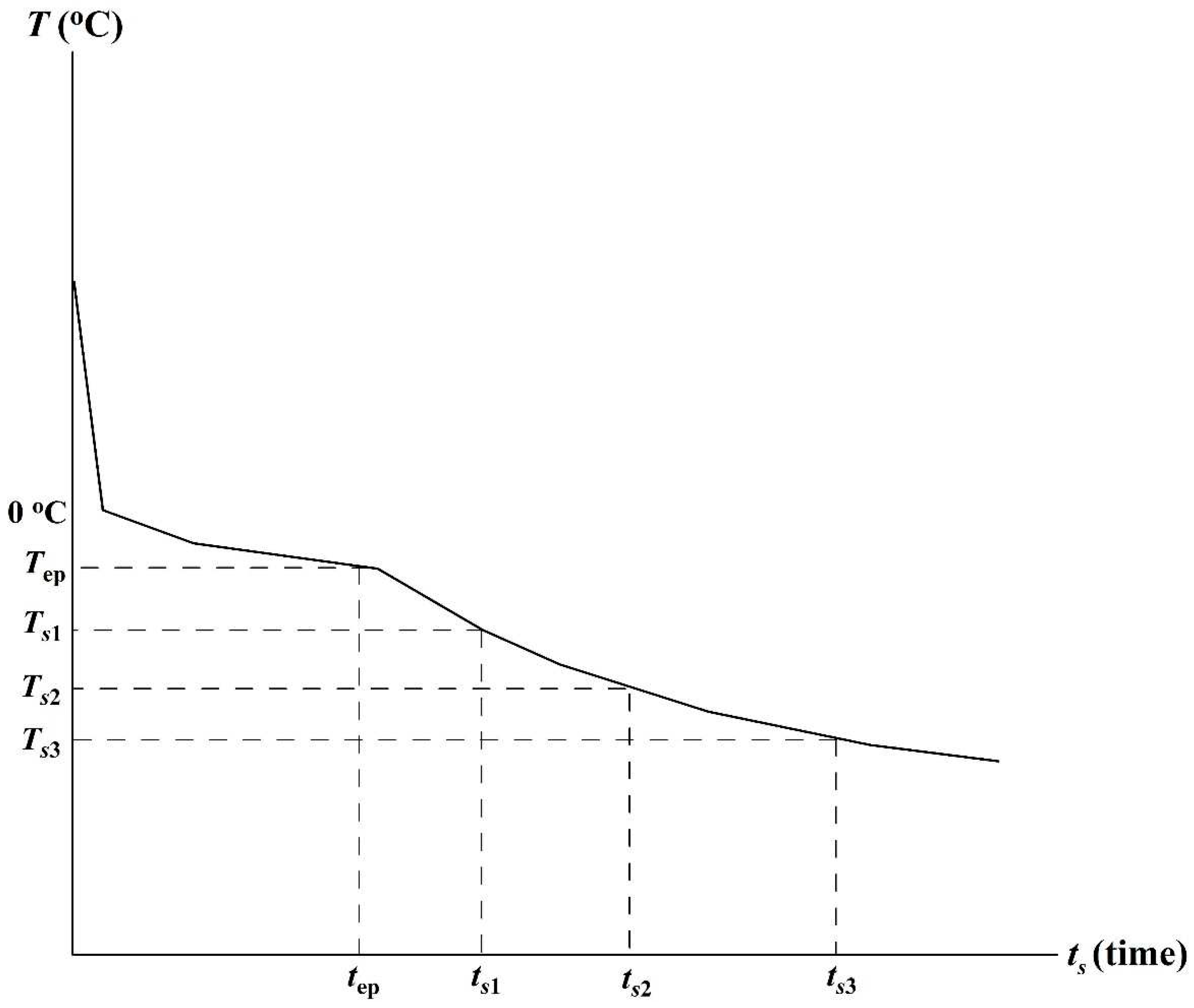
Figure 2.
Transient shut-in temperature. Case 1, B = 3.39 oC, Tfcal =-10 oC, tdD = 100, tepD = 18.5. The solid line is constructed using Eq. (1); points present the results of numerical modeling.
Figure 2.
Transient shut-in temperature. Case 1, B = 3.39 oC, Tfcal =-10 oC, tdD = 100, tepD = 18.5. The solid line is constructed using Eq. (1); points present the results of numerical modeling.
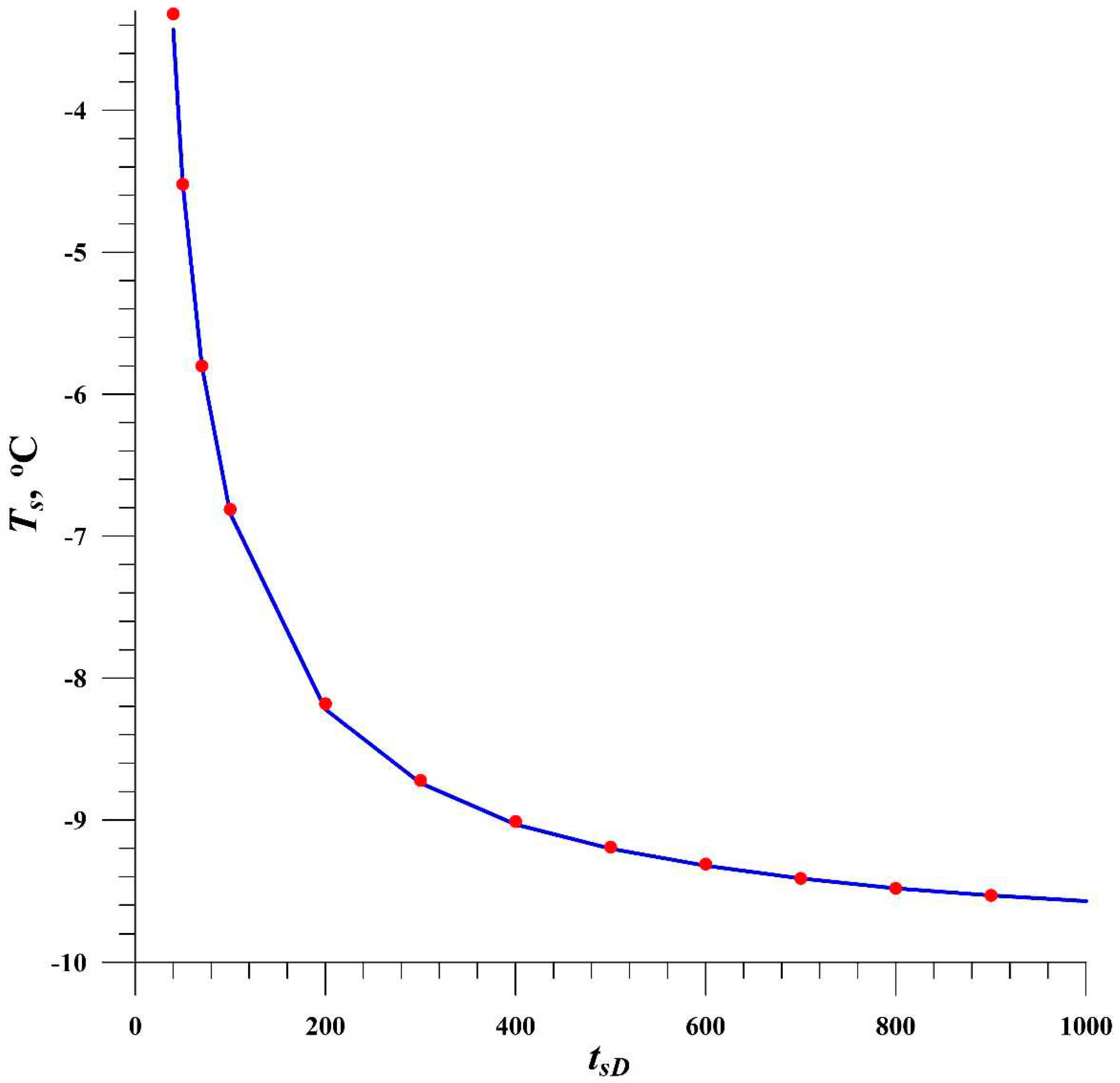

Table 1.
Input data for 2 cases of numerical modeling (Taylor, 1978, pp. 56 and 57). Tw is the temperature of the cylindrical source, Ts is the shut-in temperature, and Tf is the temperature of formation.
Table 1.
Input data for 2 cases of numerical modeling (Taylor, 1978, pp. 56 and 57). Tw is the temperature of the cylindrical source, Ts is the shut-in temperature, and Tf is the temperature of formation.
| Case 1 Tw = 10 oC, Tf = -10 oC, tdD = 100 |
Case 2 Tw = 10 oC, Tf = -10 oC, tdD = 300 |
||
| tsD | Ts, oC | tsD | Ts, oC |
|
20 30 40 50 70 100 200 300 400 500 600 700 800 900 9 |
0.00 0.00 -3.32 -4.52 -5.80 -6.81 -8.18 -8.72 -9.01 -9.19 -9.31 -9.41 -9.48 -9.53 |
30 60 90 120 150 210 300 400 500 600 700 1700 |
0.00 -1.19 -4.24 -5.29 -5.96 -6.80 -7.53 -8.02 -8.34 -8.57 -8.74 -9.47 |
Table 2.
Input data for three cases of numerical modeling (Taylor, 1978, pp. 73, 50, 65).
| tsD | Ts, oC | tsD | Ts, oC | tsD | Ts, oC |
| Case 3 Tw = 30 oC, Tf = -10 oC, tdD = 1000 |
Case 4 Tw = 10 oC, Tf = -5 oC, tdD = 30 |
Case 5 Tw =30 oC, Tf = -5 oC, tdD = 30 |
|||
| 400 500 700 800 900 1000 2000 3000 4000 5000 |
0.0 0.0 -3.52 -4.45 -5.09 -5.58 -7.93 -8.91 -9.43 -9.70 |
30 40 50 60 70 170 270 370 470 570 |
0.0 0.0 -1.22 -2.32 -2.61 -4.15 -4.46 -4.61 -4.69 -4.74 |
60 70 170 270 370 470 570 670 770 870 970 |
0.0 0.0 -2.58 -3.66 -4.05 -4.27 -4.40 -4.49 -4.56 -4.61 -4.65 |
Table 3.
Results of calculations for cases 1 and 2. Tfcal is the calculated formation temperature. Input data are presented in Table 1.
Table 3.
Results of calculations for cases 1 and 2. Tfcal is the calculated formation temperature. Input data are presented in Table 1.
| 1 | 2 | 3 | 4 | 5 | 6 | 7 | 8 | |
| ts1D | ts2D | ts3D | tepD | B,oC | Tfcal ,oC | If | Ф | |
| Case 1. H = 3.87; Tf = -10oC | ||||||||
| 50 50 50 50 50 50 50 50 40 40 40 40 40 |
70 70 70 70 70 70 70 70 70 70 70 70 70 |
900 800 700 600 500 400 300 200 200 300 400 500 600 |
18.5 18.5 18.5 18.7 18.7 18.8 19.1 19.6 21.3 20.9 20.7 20.6 20.5 |
3.49 3.50 3.49 3.46 3.46 3.45 3.43 3.37 3.25 3.31 3.34 3.35 3.36 |
-9.97 -9.97 -9.97 -9.95 -9.95 -9.95 -9.93 -9.89 -9.86 -9.91 -9.93 -9.94 -9.94 |
1.205 1.205 1.205 1.217 1.217 1.223 1.241 1.272 1.375 1.351 1.339 1.333 1.327 |
0.086 0.086 0.086 0.087 0.087 0.087 0.089 0.091 0.098 0.096 0.096 0.095 0.095 |
|
| Case 2. H = 4.80; Tf = -10 oC | ||||||||
| 90 90 90 90 90 90 90 120 120 120 120 120 |
120 120 120 120 120 120 120 210 210 210 210 210 |
210 300 400 500 600 700 1700 300 400 500 600 700 |
37.5 36.7 35.9 35.6 35.4 35.3 33.3 32.0 30.4 30.3 29.9 30.0 |
2.78 2.82 2.86 2.87 2.89 2.89 3.00 2.96 3.01 3.02 3.03 3.03 |
-9.81 -9.85 -9.89 -9.90 -9.92 -9.92 -10.02 -9.92 -9.94 -9.95 -9.95 -9.95 |
1.525 1.494 1.464 1.452 1.445 1.441 1.364 1.314 1.252 1.248 1.233 1.237 |
0.109 0.107 0.105 0.104 0.103 0.103 0.097 0.094 0.089 0.089 0.088 0.088 |
|
Table 4.
Results of calculations for cases 3-5. Tfcal is the calculated formation temperature. Input data are presented in Table 2.
Table 4.
Results of calculations for cases 3-5. Tfcal is the calculated formation temperature. Input data are presented in Table 2.
| 1 | 2 | 3 | 4 | 5 | 6 | 7 | 8 | ||||
| ts1D | ts2D | ts3D | tepD | B,oC | Tfcal ,oC | If | ф | ||||
| Case 3. H = 14.99; Tf = -10 oC | |||||||||||
| 700 700 700 700 800 800 800 800 700 |
900 900 900 900 900 900 900 900 1000 |
2000 3000 4000 5000 2000 3000 4000 5000 5000 |
382.9 348.9 336.5 338.6 334.1 291.3 277.4 282.9 311.8 |
4.16 4.62 4.98 4.77 4.56 5.10 5.29 5.22 5.02 |
-10.50 -10.81 -10.92 -10.90 -10.61 -10.90 -10.99 -10.96 -10.94 |
1.533 1.405 1.359 1.366 1.349 1.186 1.133 1.154 1.265 |
0.110 0.100 0.097 0.098 0.096 0.085 0.081 0.082 0.090 |
||||
| Case 4. H = 3.94; Tf = -5 oC | |||||||||||
| 60 170 60 270 60 370 |
570 570 570 |
45.8 46.5 48.8 |
1.11 1.09 1.00 |
-5.01 -5.01 -4.99 |
2.704 2.742 2.868 |
0.096 0.098 0.102 |
|||||
| Case 5. H = 6.42; Tf = -5 oC | |||||||||||
| 270 470 270 570 270 670 |
970 970 970 |
118.4 113.7 109.0 |
1.491 1.550 1.611 |
-4.99 -5.00 -5.00 |
2.544 2.451 2.356 |
0.091 0.088 0.084 |
|||||
Disclaimer/Publisher’s Note: The statements, opinions and data contained in all publications are solely those of the individual author(s) and contributor(s) and not of MDPI and/or the editor(s). MDPI and/or the editor(s) disclaim responsibility for any injury to people or property resulting from any ideas, methods, instructions or products referred to in the content. |
© 2023 by the authors. Licensee MDPI, Basel, Switzerland. This article is an open access article distributed under the terms and conditions of the Creative Commons Attribution (CC BY) license (http://creativecommons.org/licenses/by/4.0/).
Copyright: This open access article is published under a Creative Commons CC BY 4.0 license, which permit the free download, distribution, and reuse, provided that the author and preprint are cited in any reuse.


