

Submitted:
15 August 2023
Posted:
17 August 2023
You are already at the latest version
Abstract
In a previous paper, we solved the partial differential equation of Mullins problem in the case of the evaporation-condensation in electronic devices and gave an exact solution relative to the geometric profile of the grain boundary grooving when materials are submitted to thermal and mechanical solicitation and fatigue effect. In this new research, new modelling of the grain groove profile was proposed and new analytical expressions of the groove profile, the derivative and the groove depth were obtained in the case of diffusion in thin polycrystalline films by the resolution of the fourth differential equation formulated by Mullins that supposed 〖y'〗^2≪1. The obtained analytical solution gave more accurate information on the geometric characteristics of the groove that were necessary to study the depth and the width of the groove. These new findings will open a new way to study with more accuracy the problem of the evaporation-condensation combined to the diffusion phenomenon on the material surfaces with the help of the analytical solutions.
Keywords:
Fourth-order differential equation
; diffusion
; evaporation
; groove
; surface energy
; thermal fatigue.
; power electronic devices
Introduction
The thermal fatigue plays an important role during of degradation of interconnection compartments of power electronic devices. The temperature variations resulting from the power cycling has as consequences the stresses and plastic deformations that can affect the microstructure of the materials at the interconnection interfaces of upper metallic parts. Wires and metallization layers more solicited than silicon layers lead to the distortion of material interfaces when the temperature increases, leading to the deformation or degradation of the material surfaces. This will decrease the composite life and leads to an accelerated degradation. The arrangement of grains and grain boundaries is key to understanding the microstructure of metals and composites. When subjected to thermal and mechanical stresses, the variation in surface energies between adjacent grains, confined by the grain boundary, can cause the grains to separate. This phenomenon occurs due to the thermal and mechanical deformation of the grain boundary and the grain groove profile. Such occurrences are commonly observed in the bonding wires utilized in electronic devices.
The studies [1,2,3] have focused on examining the impact of microstructure and physicochemical properties on degradation processes. In literature [4,5,6], three effects were investigated. The first two effects examined the influence of bonding procedures and temperature on crack formation and the microstructure of the interconnection zone. Meanwhile, the third effect explored the relationship between material purity, grain size, and hardness during cycling. The metallization layer, typically around 5μm thick, deposited on the chips undergoes significant distortion compared to materials like silicon when exposed to high temperature. This distortion results in substantial tensile and compressive stresses, leading to notable inelastic strains [7]. It has been reported that thermomechanical cycling can cause two main types of degradation on the topside of power chips: metallization reconstruction and degradation of bonding contacts [7,8,9]. It is assumed that during cyclic aging, a progressive effect of condensation-evaporation occurs, leading to structural degradation and grooving of the film. However, the precise mechanism of this degradation is not yet fully understood, and further efforts are required to better comprehend the effects of stress parameters on the degradation of contacts between metallization and bond wire. This involves finding a mathematical solution to describe the formation of grain boundary grooving in polycrystalline thin films. Several solutions to this mathematical problem have been proposed in the literature [10,11,12,13,14,15,16,17,18,19,20]. In 1957, Mullins [10] conducted a study on the thermal effect on the profile of grain boundary grooving, laying the foundation for subsequent research on this phenomenon [13,14,15,16,17,18,19,20]. Various studies have focused on the development of this phenomenon, particularly exploring evaporation-condensation, surface diffusion, and formulating the mathematical problem that describes the profile of grain boundary grooving [10,11,12].Some authors [22] tried to adapt integrable nonlinear evolution equations related to the well-known linearizable diffusion equation to derive a new integrable nonlinear equation which models the surface evolution of anisotropic material accompanying the action of evaporation-condensation and surface diffusion [22].
A multiple integration technique allowing to solve high-order diffusion equations was proposed by Hristov [23] based on multiple integration procedures by applying the heat-balance integral method of Goodman and the double integration method of Volkov. Hristov [24] presented a solution for the linear diffusion models of Mullins’ thermal grooving [10,11,12].
Fourth-order diffusion equations are commonly encountered in various applications, including surface diffusion on solids [10,11,12,25,26,27,28] and thin film theory [27,28]. Unlike second-order diffusion equations, fourth-order equations generally do not satisfy any known maximum principle. Even with simple time-independent linear boundary conditions, evolving solutions tend to generate additional extrema from initially smooth conditions [29].
Broadbridge [30] studied the problem of a surface groove by evaporation-condensation governed by . The depth of a groove at a grain boundary was predicted without any approximation [30].
Chugunova and Taranets [31] studied the initial–boundary value problem associated with the fourth-order Mullins equation with initial data. They considered this problem by assuming that the specific free energy of the boundary is lower than the surface free energy. The Mullins equation, originally introduced by Mullins in 1957 [10], is a model used to analyze the evolution of surface grooves at the grain boundaries of heated polycrystals. Chugunova and Taranets [31] successfully demonstrated the global existence of weak solutions over time and established that the energy minimizing steady state serves as the global attractor.
Gurtin and Jabbour [32] developed a regularization theory that incorporates curvature effects, including surface diffusion and bulk-surface interactions. They investigated two specific cases: (i) the interface considered as a boundary between bulk phases or grains, and (ii) the interface between an elastic thin film bonded to a rigid substrate and a vapor phase depositing atoms on the surface [32].
Huang [33] conducted isothermal stress relaxation tests on electroplated Cu thin films, considering both passivated and unpassivated films. Based on a kinetic model, Huang [33] deduced grain-boundary and interface diffusivities and provided numerical and analytical solutions for the coupled diffusion problems. The study also analyzed the impact of surface and interface diffusivities on stress relaxation in polycrystalline thin films, comparing the results to experimental data.
Asai and Giga [34] considered the surface diffusion flow equation under specific boundary conditions. The problem of Mullins (1957) was proposed to model the formation of surface grooves on the grain boundaries, where the second boundary condition is replaced by zero slope condition on the curvature of the graph. Asai and Giga solved the initial-boundary problem with homogeneous initial data for construction of a self-similar solution and a solution was proposed by using a semi-divergence structure.
Escher et al. [35] demonstrated the existence and uniqueness of classical solutions for the motion of immersed hypersurfaces driven by surface diffusion. They focused the surface diffusion proposed by Mullins [10,11,12] to model surface dynamics for phase interfaces when the evolution is governed solely by mass diffusion within the interface. Other studies were devoted to the diffusion problems, grain boundary migration and grain dynamics evolution in materials [36,37,38,39,40,41,42].
Mullins et al. [43] have linearized the differential equation by assuming a very small slope at any point of the grain profile. In 1975, Brailsford & Gjostein [44] derived approximate solutions by studying the influence of surface energy anisotropy on morphological changes occurring by surface diffusion on simply shaped bodies. Wherever a grain boundary intersects the surface of a polycrystalline material, a groove develops. At the root of the groove, a balance between grain-boundary tension and surface tension produces an equilibrium angle [45]. The difference in chemical potential between the curved surface near the groove’s root and the smoother surface farther away results in material drift.
Tritscher [46] considered the boundary-value problem concerning the formation of a single groove due to surface diffusion at the junction of a bicrystal, assuming that the grain boundary remains planar.
Martin [47] extended the original Mullins theory of surface grooving due to a single interface to multiple interacting grooves formed by closely spaced flat interfaces. Martin considered two cases: the first involved simplifying Mullins’ analysis using Fourier cosine transforms instead of Laplace transforms, while the second dealt with an infinite periodic row of grooves. Martin [40] also solved the problem for two interacting grooves. Analytical solutions for the fourth partial differential equation governing the groove profile in metals have not been found in the literature.
In a previous study [48], we addressed the mathematical problem associated with the second non-linear partial differential equation in Mullin’s problem. We focused on the case of the evaporation-condensation and provided an exact solution for the geometric profile of grain boundary grooving when materials are subjected to thermal and mechanical stress, as well as fatigue effects.
This paper is devoted to model the grain groove profile governed by the fourth-order partial differential equation in the case of diffusion in thin polycrystalline films. An analytical and exact solution to the Mullins approximated problem, , was given.
Mathematical formulation in the diffusion case
In this section, we were interested to the derivation of the differential equation that describes the evolution of a two-dimensional surface of small slope under capillary driving forces and surface diffusion transport. Surface properties are assumed to be independent of orientation. For a point on the surface at which the mean curvature is c, the chemical potential μ (c) per atom can be written as
where is the chemical potential of reference for a flat surface (c = 0), γ is the surface tension of the metal/vapor interface and ω is the atomic volume of the film material. A gradient of surface curvature will therefore create a gradient of the chemical potential, which will produce a drift of atoms on the surface with an average velocity v given by the Nernst-Einstein relation.
where Ds is the surface diffusivity, k is the Boltzmann constant and T the absolute temperature.
The surface current of atoms JS is defined by the product of the average velocity v by the atom number NS per unit surface area S, it is given by the following equation:
The evolution of the surface may finally be described by the speed of movement vn, of the surface element along its normal:
Notice that is the number of diffusing atoms per unit area, the surface current of atoms and B a rate constant given by the following equation:
Equation (7) can be written in the general case as:
If y is the coordinate of a point at the surface along the axis normal to the initial flat surface, the speed of motion of the point along this axis vn is obtained by projection on the y-axis and one obtains:
Combining equations (9) and (10), one obtains:
Knowing that the curvature c is given by the following expression:
and
One obtains:
Using the same method for , one obtains:
Therefore:
With and , previous equation can be written as:
With the following boundary conditions:
Knowing that
One obtains:
By taking the following variable changes:
One obtains the different derivatives of and :
with
Equation (25) becomes:
or
By using the previous equations, one obtains:
With equation (20):
One writes:
Let us put:
Using equation (32), one obtains:
New study of Mullins’s case
If we suppose a second order approximation of the derivative, , it is easy to deduce the following equation:
With the new boundary conditions:
Exact resolution of Mullins’ problem
In this section, we propose a new method to resolve the equation (38) by using the following equation:
and by considering the different solutions r in function of u.
Let us consider the following equation valid for all values of :
To resolve equation (38), we begin by transforming equation (39’) into difference between two perfect squares, therefore, the expression will be transformed into perfect square, if it has a double solution and then his discriminant has to be cancelled.
Now, let us consider the equation:
The discriminant of this second-degree equation (40) function in r can be written as:
Putting , one has:
Equation (42) can be written as:
With and Putting and taking or one obtains ; and et will be the two solutions of the following second-degree equation:
or
The discriminant of equation (44′):
Can be calculated as a function of u:
Two cases have to be distinguished:
- 1.
- First case and
In this case, the solutions of equation (44′) will be given by:
This leads to the solution of equation (43):
This value of will cancel the discriminant of equation (40)
Therefore, the solution r is given by:
and then:
Consequently, one obtains:
or
The four solutions of equation (37) can be then obtained from the solutions of the two following 2nd degree equations:
The discriminants of equations (53) and (54) are given by the respective following expressions:
Two cases can be studied:
Solutions of
Knowing that is negative because of the condition , one obtains two conjugate complex solutions:
Solutions of
Where
Let us prove that
can be written as: , To obtain the sign of , we have to study the sign of and then to compare between 1 and or between and .
Let us put , one obtains:
Equation (61) shows that , this implies that Z decreases for all values of and for and therefore or and .
Therefore, the two other solutions are then given by equations (62) and (63):
Solution of equation (38) for
Now, the final solution, in the case of , is given by equation (64):
with
The solution in function of will be written as:
Boundary conditions
Using of the boundary conditions:
The first condition implies necessary: A3 = A4 = 0 and therefore the solution will be given by the following form:
This solution can be written as:
With
- 2.
- Second case and
In this case, one obtains two conjugate complex solutions and :
Where and and finally With:
The real solution is given by:
or
This leads to the solution of equation (43):
This value of λ will cancel the discriminant of equation (39)
The solution is given here by:
Remember that:
And therefore:
Their respective discriminants are given below:
Two cases can be studied for
:
First case:
Here one has
Where is negative. The two conjugate complex solutions of equation (53) are given below:
Second case:
Here one has and
Let us prove that is negative
can be written as:
Knowing that ; or therefore, one obtains:
Now, one writes: and one obtains:
It is obvious that and then , therefore
The two other conjugate complex solutions are then given by equations (75) and (76)
Now, the final solution in this case when is negative or when is given by:
One obtains:
where:
The continuity and derivability of the solution g(u) and its derivatives imposed that
Because the function is not derivable in point and then, one writes:
In conclusion, one obtains the solutions of the fourth differential equation (37):
For :
For :
With
Satisfying the boundary conditions:
Determination of the problem parameters of the solution for
With the boundary conditions and knowing that for u = 0, ; and one obtains:
Where is the groove depth.
Condition on the first derivative
The calculation of the first derivative gave:
with
Knowing that ; and , one obtains: ; ; and then the first derivative :
At u = 0, ; ; ; , one obtains , and then ; ; and .
The use of the above parameters led to:
The second derivative
One had the second derivative:
To determine the values of and , one needs to determine the second derivative .
The second derivative ; let’s put ; therefore,
Knowing that: , one obtains:
By using , one obtains: and therefore:
The other second derivatives are given below:
By calculating the values of the second derivatives at point u = 0: ; ; ; one obtains the following equation:
And then:
Condition on the second derivative
The calculation of the third derivative led to:
Let us calculate the third derivative
:
Using , one obtains:
By using relation: , one obtains:
And finally, one obtains the third derivative :
One also calculated the other derivatives:
and
Knowing that the fourth boundary condition and the values of the third derivatives at point u = 0: ; ; ; ; one obtains the following equation:
, therefore:
Consequently, the use of the boundary conditions gave the following linear system composed by four equations with four unknown parameters:
And the the function g and its different derivatives are given at point 0:
Therefore, the solution for is completely defined by all above parameters:
The values of the different parameters and their derivatives at point were calculated:
Determination of the problem constants of the solution for
In this case, on has , with given by:
The values of the different parameters of the solution and their derivatives at point are given below:
One proved that all parameters and derivatives for the two functions and are equal and the continuity of the solution and its derivatives is assured, at this point and consequently at any point of the interval [0, ∞], for:
Now the analytical solution of the fourth order differential equation was completely given and all problem constants were determined.
with
With and , the solution can be written as:
Profile of the groove shape in the diffusion case
The variations of the profile as a function of the distance x from the symmetric axis of the groove are plotted on Figure 1.
The study of the solution reveals a damped sinusoidal profile of the groove with an infinity of maxima, minima and zeros of the solutions. The oscillations can be easily observed in our solution. Mullins mentioned that it is questionable, however, that these oscillations could be observed due to the progressively decreasing amplitude of g. Here, we proved the superiority of our analytical solution that can predict the all oscillations, their amplitudes, the zero, the maxima and minima of the groove profile.
As example, we gave on Table 1 the 12 first values of the groove shape parameters and on Table 2 the distance between two consecutive maxima and minima for the first 12 numbers.
We observed that decreases towards zero when x increases to the infinity as well as the absolute value of (Table 1). This will decrease the distance between two consecutive maxima and minima when the distance x increases.
Equations given in Table 3 showed the properties of damped sinusoidal functions and the pseudo-periodicity of the various groove parameters and the strong correlations between them showing at the same time the infinity of the number of these different parameters.
On Table 4, we gave the various results obtained by our analytical solution and the Mullins’s results.
The parabolic approximation of the groove profile obtained by Mullins was valid for , whereas, our approximation more precise is valid for (from the origin until the first maximum of the groove shape). On the other hand, the error committed by Mullins calculations on the abscissa of the first maximum the zero of the function y and the first inflexion point is about 7%, while that on the ordinate of the profile maximum exceeds 25%. On Table 4, we were able, on the contrary of Mullins results, to give more information on the various maxima, minimas, zeros and positive and negative inflexion points of the grove shape profile.
If we notice and the depths of the groove taken from the bottom of the grove respectively to its first maximum and minimum, one can write:
Now, knowing that
and
One deduced:
and
The separation distance between two consecutive maxima or minima was given in Table 2 proving the variation of this distance as a function of optima number N. One obtained the interpolated expressions on Table 5:
Table 5 clearly showed that the ratio is independent from the time, for example, we can give this ratio for the first maximum:
Table 6 showed a certain deviation of Mullins results with respect to those of the analytical solution proposed in this paper, that can reach 12% in the case of the first maximum of the groove shape. However, Mullins did not give any additional information on the other maxima, minima, zeros of the solution and the various inflexion points, while our solution gave more complete information on the different parameters of the groove and also proposed many correlations that can be very useful for the readers.
Here, some information on the coordinates of the positive and negative inflexion points are given on Table 7.
Competition between evaporation and diffusion
When studying the evolution of grain boundary groove profiles in the cases of the evaporation/condensation and surface diffusion, Mullins [10] assumed that: (1) the surface diffusivity and the surface energy, , were independent of the crystallographic orientation of the adjacent grains and (2) the tangent of the groove root angle, γ, is small compared to unity. Mullins also supposed an isotropic material. The assumption (tanθ << 1) was used in all papers’ Mullins to simplify the study of the mathematical partial differential equation. The polycrystalline metal was supposed (3) in quasi-equilibrium with its vapor. The interface properties don’t depend on the orientation relative to the adjacent crystals. The grooving process was described by Mullins using the macroscopic concepts (4) of surface curvature and surface free energy. The matter flow (5) is neglected out of the grain surface boundary.
The mathematical equation governing the evaporation-condensation problem can be written here as:
where C(T) a constant of the problem depending on the temperature T, given by:
where γ is the isotropic surface energy, the vapor pressure at temperature T in equilibrium with the plane surface of the metal characterized by a curvature c = 0, ω is the atomic volume, m is molecular mass, μ the coefficient of evaporation and k is the Boltzmann constant.
We remember here the analytical solution of the evaporation case without any approximation [our paper] given by
and
By combining the two phenomena of diffusion and evaporation/condensation, one writes:
With the approximation postulated by Mullins supposing that one can write:
With
Let’s put the profile area. One can write the rate of change of profile area:
One writes:
The Mullins’ approximation supposed that and . In a previous paper [ref], we studied the case of evaporation without this approximation and obtained at the origin the following relations:
In such case, on obtains:
And
This relationship provides clear evidence that the rate of change of the profile area is influenced by both evaporation and diffusion, contrary to Mullin’s prediction which states that and is independent of surface diffusion.
Calculation of the profile area
from below to above the original surface
By using the differential equation:
One writes:
Where is the first zero of the function g.
Therefore:
And:
If σ is the profile area transferred from below to above of the original surface by surface diffusion alone divided by the profile area lost by evaporation, one can write:
With , one has and one deduces:
If we suppose that the contact angle is small or (for Theta < 18°) we obtain:
Our relation proved that depends on the temperature, at contrary of the relation obtained by Mullins:
Indeed, in this relation, there is no direct effect of the temperature. To compare between the two previous expressions, we supposed that and obtained:
This calculation yielded a ratio of , indicating an overestimation compared to the value proposed by Mullins. Table 8 and Table 9 provide two examples comparing the results obtained using the two methods for Au and Mg metals.
We observed that the profile areas corresponding to Au and Mg are overestimated by the Mullins method (about 2.5 times greater than our new values). On the other hand, the calculated ratio of the profile area lost by evaporation of Au and Mg is equal to:
This proved that whatever the time, the evaporation of Au is times more important than that of Mg. However, the diffusion of Mg particles is greater than that of Au.
The same procedure was used to determine the values of the profile area lost by evaporation of some common metals (Table 10).
These interesting results of the Table 10 gave the following order of the various metals by increasing profile area:
Cu < Al < Sr < Li < Cs < Ti < Co < Ga < Tl
On Table 11, we gave the obtained values of the two constants C and B of evaporation and diffusion for the different metals.
The constant of evaporation C decreases from the cobalt element Co to cesium by respecting the following increasing order:
Co < Ti < Ga < Li < Tl < Al < Cu < Sr <Cs
Whereas, this order changes for the constant of diffusion that increases from Cu to Cs with the following order:
Cu < Co < Ga < Li < Ti < Al < Tl < Sr <Cs
Another important conclusion concerns the larger value of constant C with respect to B. It is shown that the value of C is about 1012 times greater that of B. This led to conclude that the diffusion can be neglected relative to evaporation.
The depth of the groove
In many experiments, it was proved that the depth groove can vary from 0.1mm to several 10 mm in the case of diffusion depending on the metal thermal properties and on the width of the groove. In order to understand the thermal behavior of diffusion of the various elements, let’s take the typical example where m = 0.20 and calculate the corresponding depth of the groove for metals (Table 12).
Knowing that the width of the groove is given by:
One deduced the value of for the different metals presented on Table 13.
Consequences of the new solution
The experimental study of the geometric characteristics of the groove for metals can lead to the determination of the two constants of evaporation and diffusion. Indeed, the evaporation constant can be obtained by determining experimentally the value of the profile area and by considering in first approximation and therefore is given by:
By determining the value of C, it becomes possible to determine the surface energy γ of the metal using the relation of the evaporation constant, resulting in the following expression:
The evaluation of the width of the groove will give the value of diffusion constant by using our previous relation:
And therefore:
Knowing γ and , we will be able to obtain the value of the surface diffusion :
Validity of the approximation of
Let’s consider the case of copper metal to test the validity of and draw on Figure 3 the variations of as a function of the distance x for different contact angles.
Figure 3 showed that for θ < 30°, the value of <0.2 and can be approximately neglected behind 1 following Mullins’ approximation. Therefore, for θ > 30°, the approximated fourth partial differential equation proposed by Mullins cannot be used for the diffusion case and then it will be necessary to resolve the non-linear partial fourth order differential equation that cannot be analytically obtained.
Variations of the groove profile y(x) and the derivative y'(x)as a function of the distance x of Cu
We used the results of our analytical solution to determine the groove profile and its derivative in the case of copper metal. On Figure 4, we drew the variations of the profile y(x) and y'(x) in the case of Cu by noting the geometric parameters of the groove such as , and . By using our solution, we obtained the following geometric characteristics of the groove:
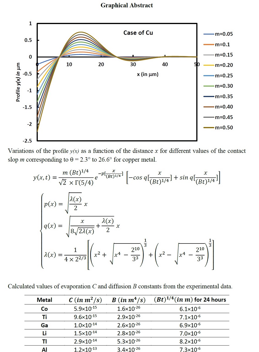
On Figure 5, we plotted the variations of the profile y(x) of the groove of Cu as a function of the distance x for different values of contact angles.
Figure 5 clearly showed the effect of the contact angle of the grove. The groove depth increases when m increases. However, the other characteristics such as and remain the same.
The obtained analytical solution allowed to compare between the groove profiles among various metals. Figure 6 showed different groove characteristics in different metals. It can be seen that the groove depth and the distance between two maxima increased from Cu to Cs
Figure 6 also showed the large difference in the behavior of the various metals. The grove phenomenon is more accentuated for Cs, whereas, Cu is the less affected by the surface diffusion.
Conclusion
In this study, we have derived an exact solution to the partial differential equation . The obtained solution reveals a damped sinusoidal groove profile in the case of electronic power devices. We have provided expressions of zeros, minima, and maxima of the profile as a function of the order number, as well as detailed information about the groove profile y(x) and its derivatives. A comprehensive comparison with Mullins’ results was conducted, demonstrating that Mullins’ predictions significantly overestimate the geometric characteristics of the groove, exceeding the actual values by more than 2.5 times. Additionally, valuable insights into the diffusion behavior of various metals gained through this study. The expressions for the evaporation and diffusion constants and coefficients were also derived, accounting for the groove parameters.
Conflicts of Interest
“The authors declare no conflict of interest.”
Appendix A
Variations of the profile y(x) as a function of the distance x for different values of the contact slop m corresponding to θ = 2.3° to 26.6° for copper metal.
Calculated values of evaporation C and diffusion B constants from the experimental data.
| Metal | for 24 hours | ||
| Co | 5.9×10⁻¹⁵ | 1.6×10⁻²⁶ | 6.1×10⁻⁶ |
| Ti | 9.6×10⁻¹⁵ | 2.9×10⁻²⁶ | 7.1×10⁻⁶ |
| Ga | 1.0×10⁻¹⁴ | 2.6×10⁻²⁶ | 6.9×10⁻⁶ |
| Li | 1.5×10⁻¹⁴ | 2.8×10⁻²⁶ | 7.0×10⁻⁶ |
| Tl | 2.9×10⁻¹⁴ | 5.3×10⁻²⁶ | 8.2×10⁻⁶ |
| Al | 1.2×10⁻¹³ | 3.4×10⁻²⁶ | 7.3×10⁻⁶ |
| Cu | 1.7×10⁻¹³ | 1.2×10⁻²⁶ | 5.7×10⁻⁶ |
| Sr | 2.4×10⁻¹³ | 1.4×10⁻²⁵ | 1.0×10⁻⁵ |
| Cs | 2.8×10⁻¹³ | 2.7×10⁻²⁵ | 1.2×10⁻⁵ |
References
- G. P. Zhang, C. A. G. P. Zhang, C. A. Volkert, R. Schwaiger, R. Mönig, and O. Kraft, “Fatigue and thermal fatigue damage analysis of thin metal films,” Microelectron. Reliab., vol. 47, pp. 2007–2013, 2007.
- Zaefferer, S.; Kuo, J.-C.; Zhao, Z.; Winning, M.; Raabe, D. On the influence of the grain boundary misorientation on the plastic deformation of aluminum bicrystals. Acta Mater. 2003, 51, 4719–4735. [Google Scholar] [CrossRef]
- D. Martineau, C. D. Martineau, C. Levade, M. Legros, P. Dupuy, and T. Mazeaud, “Microelectronics Reliability Universal mechanisms of Al metallization ageing in power MOSFET devices,” Microelectron. Reliab., vol. 54, pp. 2432–2439, 2014.
- Broll, M.S.; Geissler, U.; Höfer, J.; Schmitz, S.; Wittler, O.; Lang, K.D. Microstructural evolution of ultrasonic-bonded aluminum wires. Microelectron. Reliab. 2015, 55, 961–968. [Google Scholar] [CrossRef]
- W. Loh, M. W. Loh, M. Corfield, H. Lu, S. Hogg, T. Tilford, and C. M. Johnson, “Wire Bond Reliability for Power Electronic Modules - Effect of Bonding Temperature,” in Thermal, Mechanical and Multi-Physics Simulation Experiments in Microelectronics and Micro-Systems, 2007, p. 6.
- Agyakwa, P.A.; Yang, L.; Arjmand, E.; Evans, P.; Corfield, M.R.; Johnson, C.M. Damage Evolution in Al Wire Bonds Subjected to a Junction Temperature Fluctuation of 30 K. J. Electron. Mater. 2016, 45, 3659–3672. [Google Scholar] [CrossRef]
- H. K. Tseng and M. L. Wu, “Electro-thermal-mechanical modeling of wire bonding failures in IGBT,” Proc. Tech. Pap. - Int. Microsystems, Packag. Assem. Circuits Technol. Conf. IMPACT, pp. 152–157, 2013. [CrossRef]
- Medjahed, H.; Vidal, P.-E.; Nogarede, B. Thermo-mechanical stress of bonded wires used in high power modules with alternating and direct current modes. Microelectron. Reliab. 2012, 52, 1099–1104. [Google Scholar] [CrossRef]
- Mullins, W.W. Theory of linear facet growth during thermal etching. Philos. Mag. 1961, 6, 1313–1341. [Google Scholar] [CrossRef]
- Mullins, W.W. Theory of Thermal Grooving. J. Appl. Phys. 1957, 28, 333–339. [Google Scholar] [CrossRef]
- Mullins, W. The effect of thermal grooving on grain boundary motion. Acta Met. 1958, 6, 414–427. [Google Scholar] [CrossRef]
- W. W. Mullins, Grain boundary grooving by volume diffusion, Transactions of the Metallurgical Society of AIME, 218, 354-361, 1960.
- H. Zhang and H. Wong, Coupled grooving and migration of inclined grain boundaries: regime I, Acta Materialia, 50, 1983–1994, 2002.
- Bouville, M.; Chi, D.; Srolovitz, D.J. Grain-Boundary Grooving and Agglomeration of Alloy Thin Films with a Slow-Diffusing Species. Phys. Rev. Lett. 2007, 98, 085503–085503. [Google Scholar] [CrossRef] [PubMed]
- Bouville, M. Effect of grain shape on the agglomeration of polycrystalline thin films. Appl. Phys. Lett. 2007, 90. [Google Scholar] [CrossRef]
- Génin, F.; Mullins, W.; Wynblatt, P. The effect of stress on grain boundary grooving. Acta Met. et Mater. 1993, 41, 3541–3547. [Google Scholar] [CrossRef]
- S. A. Hackney, Grain-boundary grooving at Þnite grain size, Scripta Metall. 22, 1731, 1988.
- L. Klinger, E. L. Klinger, E. Glickman, V. Fradkov, W. Mullins, and C. Bauer, Extension of thermal grooving for arbitrary grain-boundary ßux, J. Appl. Phys. 78, 3833-3838, 1995.
- Klinger, L.M.; Glickman, E.E.; Fradkov, V.E.; Mullins, W.W.; Bauer, C.L. Effect of Surface and Grain-Boundary Diffusion on Interconnect Reliability. MRS Proc. 1995, 391. [Google Scholar] [CrossRef]
- Brokman, A.; Kris, R.; Mullins, W.; Vilenkin, A. Analysis of boundary motion in thin films. Scr. Met. et Mater. 1995, 32, 1341–1346. [Google Scholar] [CrossRef]
- H. A. Stone, M. J. H. A. Stone, M. J. Aziz, and D. Margetis, Grooving of a grain boundary by evaporation–condensation below the roughening, Journal of Applied Physics 97, 113535-1-6, 2005.
- P. Tritscher, An integrable fourth-order nonlinear evolution equation applied to surface redistribution due to capillary, J. Austral. Math. Soc. Ser. B. 1997, 38, 518–541.
- Hristov, J. Multiple integral-balance method: Basic idea and an example with Mullin’s model of thermal grooving. Therm. Sci. 2017, 21, 1555–1560. [Google Scholar] [CrossRef]
- Hristov, J. Fourth-order fractional diffusion model of thermal grooving: integral approach to approximate closed form solution of the Mullins model. Math. Model. Nat. Phenom. 2018, 13, 6. [Google Scholar] [CrossRef]
- Tritscher, P.; Broadbridge, P. Grain boundary grooving by surface diffusion: an analytic nonlinear model for a symmetric groove. 1995, 450, 569–587. [CrossRef]
- Schwartz, L.W.; Roy, R.V. Theoretical and numerical results for spin coating of viscous liquids. Phys. Fluids 2004, 16, 569–584. [Google Scholar] [CrossRef]
- Myers, T.G. Thin Films with High Surface Tension. SIAM Rev. 1998, 40, 441–462. [Google Scholar] [CrossRef]
- Tritscher, P. An integrable fourth-order nonlinear evolution equation applied to surface redistribution due to capillarity. J. Aust. Math. Soc. Ser. B. Appl. Math. 1997, 38, 518–541. [Google Scholar] [CrossRef]
- Broadbridge, P. Entropy Diagnostics for Fourth Order Partial Differential Equations in Conservation Form. Entropy 2008, 10, 365–379. [Google Scholar] [CrossRef]
- Broadbridge, P. Exact solvability of the Mullins nonlinear diffusion model of groove development. J. Math. Phys. 1989, 30, 1648–1651. [Google Scholar] [CrossRef]
- Chugunova, M.; Taranets, R. Existence and long-time behaviour of weak solutions for the Mullins equation. Nonlinear Anal. Theory, Methods Appl. 2012, 75, 6550–6561. [Google Scholar] [CrossRef]
- Gurtin, M.E.; Jabbour, M.E. Interface Evolution in Three Dimensions¶with Curvature-Dependent Energy¶and Surface Diffusion:¶Interface-Controlled Evolution, Phase Transitions, Epitaxial Growth of Elastic Films. Arch. Ration. Mech. Anal. 2002, 163, 171–208. [Google Scholar] [CrossRef]
- Huang, R.; Gan, D.; Ho, P.S. Isothermal stress relaxation in electroplated Cu films. II. Kinetic modeling. II. Kinetic modeling. J. Appl. Phys. 2005, 97. [Google Scholar] [CrossRef]
- Asai, T.; Giga, Y. On self-similar solutions to the surface diffusion flow equations with contact angle boundary conditions. Interfaces Free. Boundaries 2014, 16, 539–573. [Google Scholar] [CrossRef]
- Escher, J.; Mayer, U.F.; Simonett, G. The Surface Diffusion Flow for Immersed Hypersurfaces. SIAM J. Math. Anal. 1998, 29, 1419–1433. [Google Scholar] [CrossRef]
- Simonnin, P.; Schreiber, D.K.; Uberuaga, B.P.; Rosso, K.M. Atomic diffusion, segregation, and grain boundary migration in nickel-based alloys from molecular dynamics simulations. Mater. Today Commun. 2023, 35. [Google Scholar] [CrossRef]
- Beyerlein, I.; Caro, A.; Demkowicz, M.; Mara, N.; Misra, A.; Uberuaga, B. Radiation damage tolerant nanomaterials. Mater. Today 2013, 16, 443–449. [Google Scholar] [CrossRef]
- Liu, Y.; Wang, Q.; Chen, L.; Xiao, Z.; Fan, X.; Ma, S.; Ming, L.; Tayal, A.; Zhang, B.; Wu, F.; et al. Diffusion-induced stress optimization by boosted surface Li-concentration for single-crystal Ni-rich layered cathodes. Mater. Today 2022, 61, 40–53. [Google Scholar] [CrossRef]
- Wang, H.; Chao, Q.; Cui, X.; Chen, Z.; Breen, A.; Cabral, M.; Haghdadi, N.; Huang, Q.; Niu, R.; Chen, H.; et al. Introducing C phase in additively manufactured Ti-6Al-4V: A new oxygen-stabilized face-centred cubic solid solution with improved mechanical properties. Mater. Today 2022, 61, 11–21. [Google Scholar] [CrossRef]
- Wei, H.-X.; Tang, L.-B.; Huang, Y.-D.; Wang, Z.-Y.; Luo, Y.-H.; He, Z.-J.; Yan, C.; Mao, J.; Dai, K.-H.; Zheng, J.-C. Comprehensive understanding of Li/Ni intermixing in layered transition metal oxides. Mater. Today 2021, 51, 365–392. [Google Scholar] [CrossRef]
- Li, H.; Tian, C.; Wang, L.; Mo, Y.; Li, J.; Wang, C.; Li, C.; Zheng, L.; Huang, F.; Li, Q. Insight into the Co/Fe intrinsically assembled structure in cobalt-iron-layered double hydroxides on catalytic oxygen evolution reaction. Mater. Today Energy 2023, 35. [Google Scholar] [CrossRef]
- Chen, N.; Liu, H.; Yang, C.; Liu, H.; Chen, J.; Dai, Y.; Yang, P.; Feng, Y.; Gui, W.; Peng, W.; et al. A multi-particle cellular automaton modeling method for grain dynamics evolution of nickel-rich cathode material. Mater. Today Energy 2023, 35. [Google Scholar] [CrossRef]
- Mullins, W.W.; Sekerka, R.F. Morphological Stability of a Particle Growing by Diffusion or Heat Flow. 1999, 75–81. [CrossRef]
- Brailsford, A.D.; Gjostein, N.A. Influence of surface energy anisotropy on morphological changes occurring by surface diffusion. J. Appl. Phys. 1975, 46, 2390–2397. [Google Scholar] [CrossRef]
- Bailey, G.L.J.; Watkins, H.C. Surface Tensions in the System Solid Copper-Molten Lead. Proc. Phys. Soc. Sect. B 1950, 63, 350–358. [Google Scholar] [CrossRef]
- Peter Tritscher “Thermal Grooving by Surface Diffusion for an Extended Bicrystal Abutting a Half-Space.” Proceedings: Mathematical, Physical and Engineering Sciences, vol. 455, no. 1986, 1999, pp. 1957–77. JSTOR. https://www.jstor.org/stable/53309. Accessed 17 Apr. 2023.
- Martin, P. Thermal grooving by surface diffusion: Mullins revisited and extended to multiple grooves. Q. Appl. Math. 2009, 67, 125–136. [Google Scholar] [CrossRef]
- Hamieh, T.; Khatir, Z.; Ibrahim, A. New solution of the partial differential equation of the grain groove profile problem in the case of evaporation/condensation. Sci. Rep. 2019, 9, 1–17. [Google Scholar] [CrossRef]
Figure 1.
Groove profile giving as a function of the distance from the symmetric axis of the groove.
Figure 1.
Groove profile giving as a function of the distance from the symmetric axis of the groove.
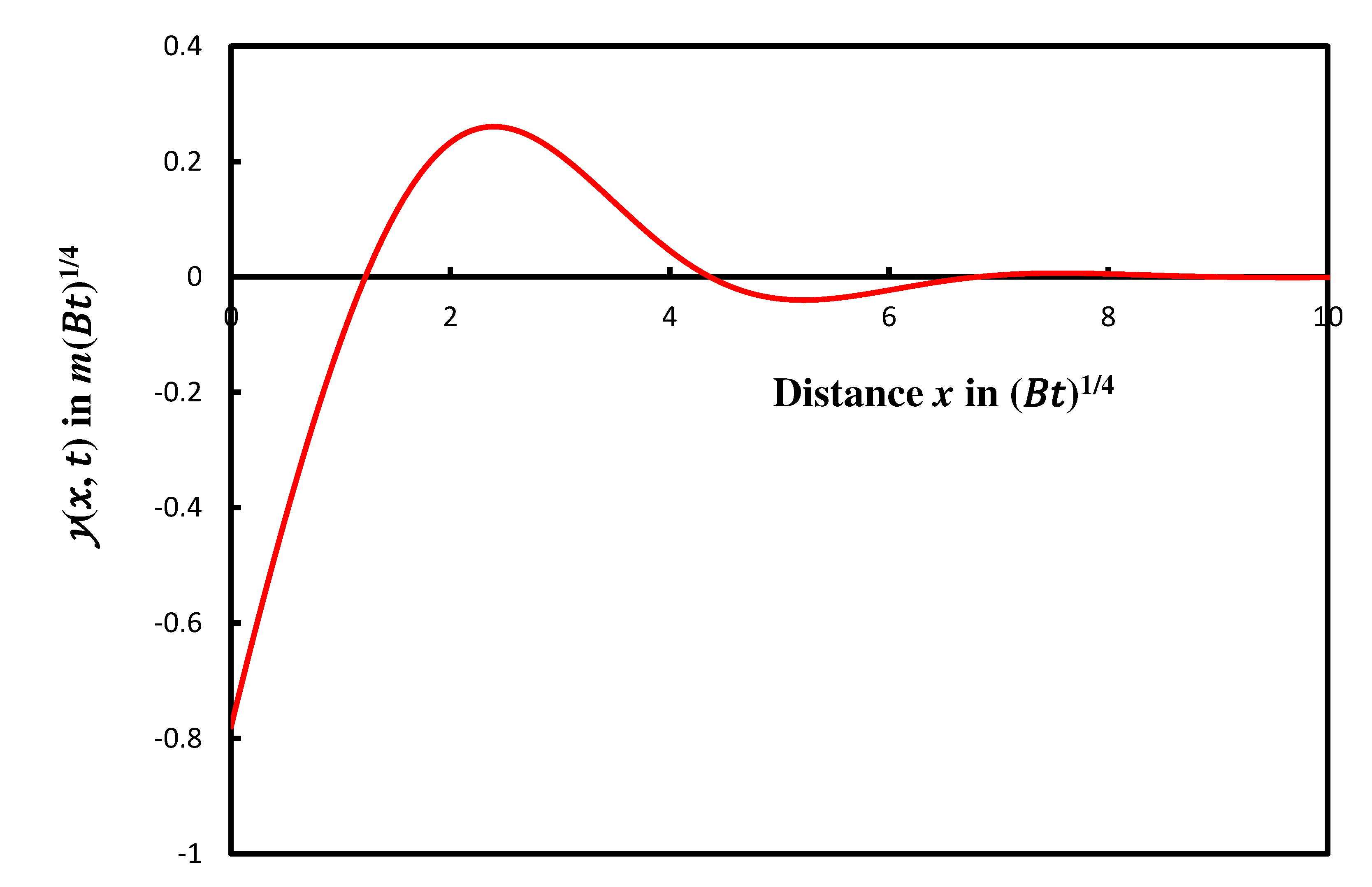
Figure 2.
Curves of interpolation of the parameters of the grove as a function of the parameter number N.
Figure 2.
Curves of interpolation of the parameters of the grove as a function of the parameter number N.
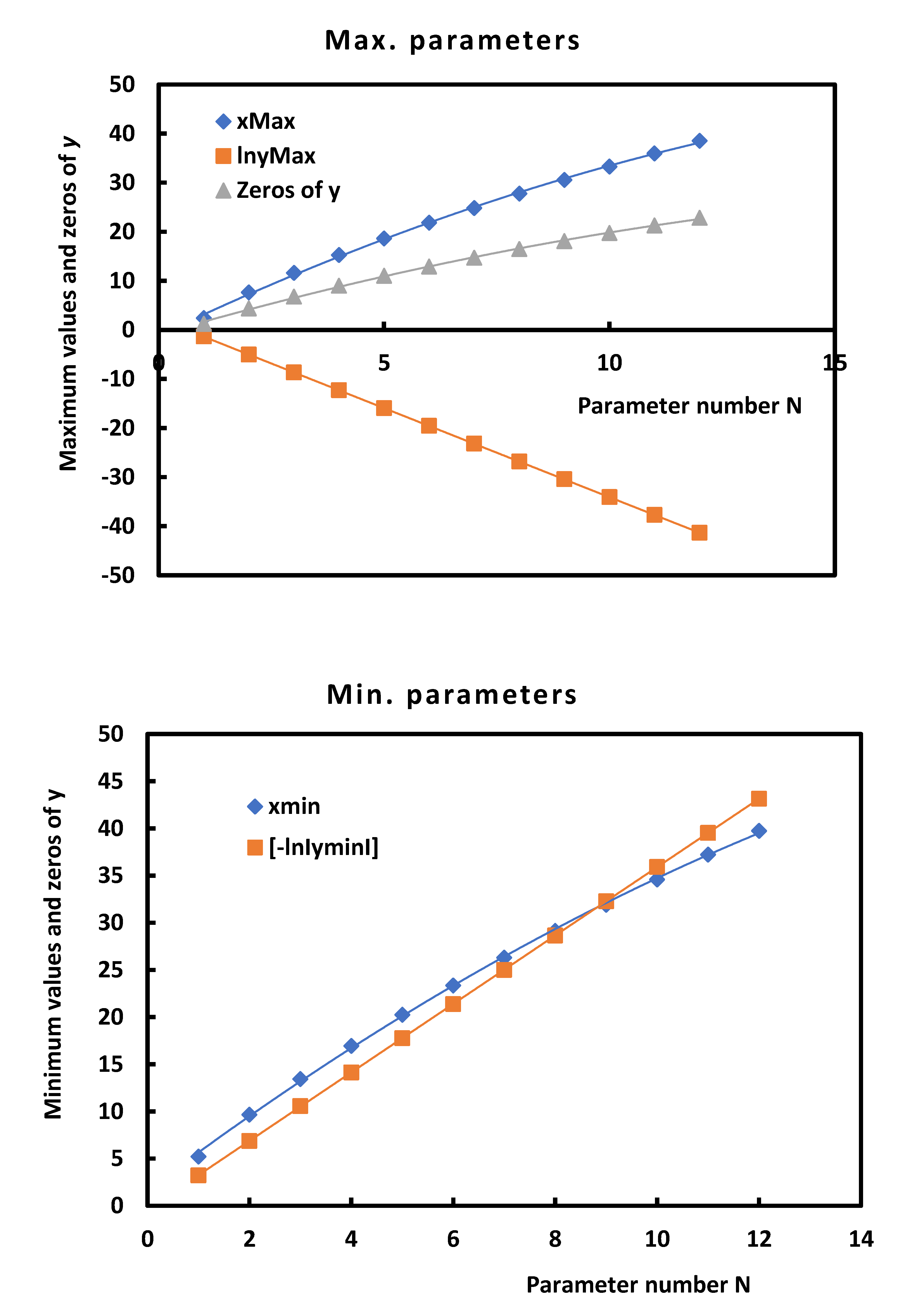
Figure 3.
Variations of as a function of the distance x from the symmetrical axis of the groove at different contact angles (θ from 1° to 70 ° and m from 0.017 to 2.75) in the case of copper element.
Figure 3.
Variations of as a function of the distance x from the symmetrical axis of the groove at different contact angles (θ from 1° to 70 ° and m from 0.017 to 2.75) in the case of copper element.
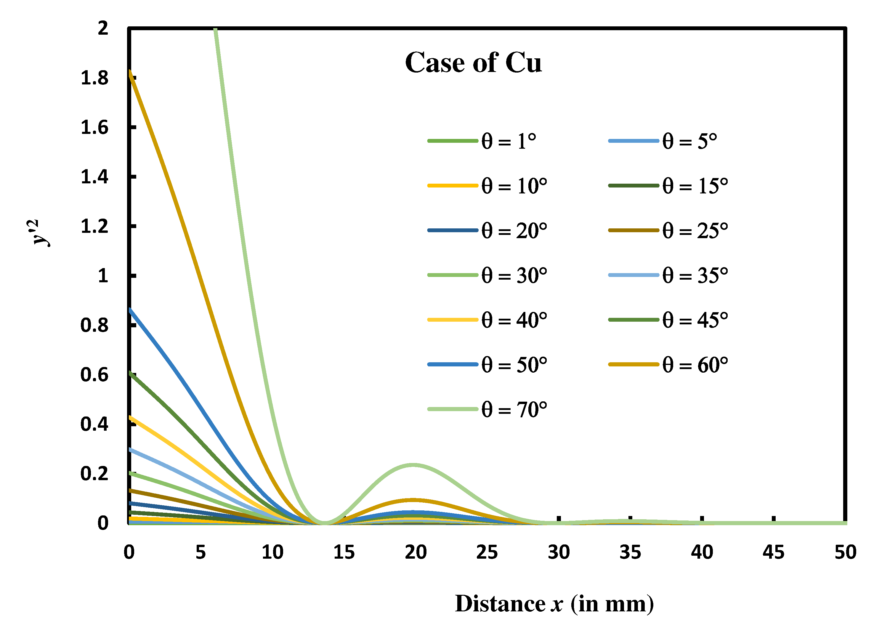
Figure 4.
Variations of the profile y(x) and y'(x) as a function of the distance x from the symmetrical axis of the groove when θ = 20° (m = 0.364) for copper metal with the geometric characteristics.
Figure 4.
Variations of the profile y(x) and y'(x) as a function of the distance x from the symmetrical axis of the groove when θ = 20° (m = 0.364) for copper metal with the geometric characteristics.
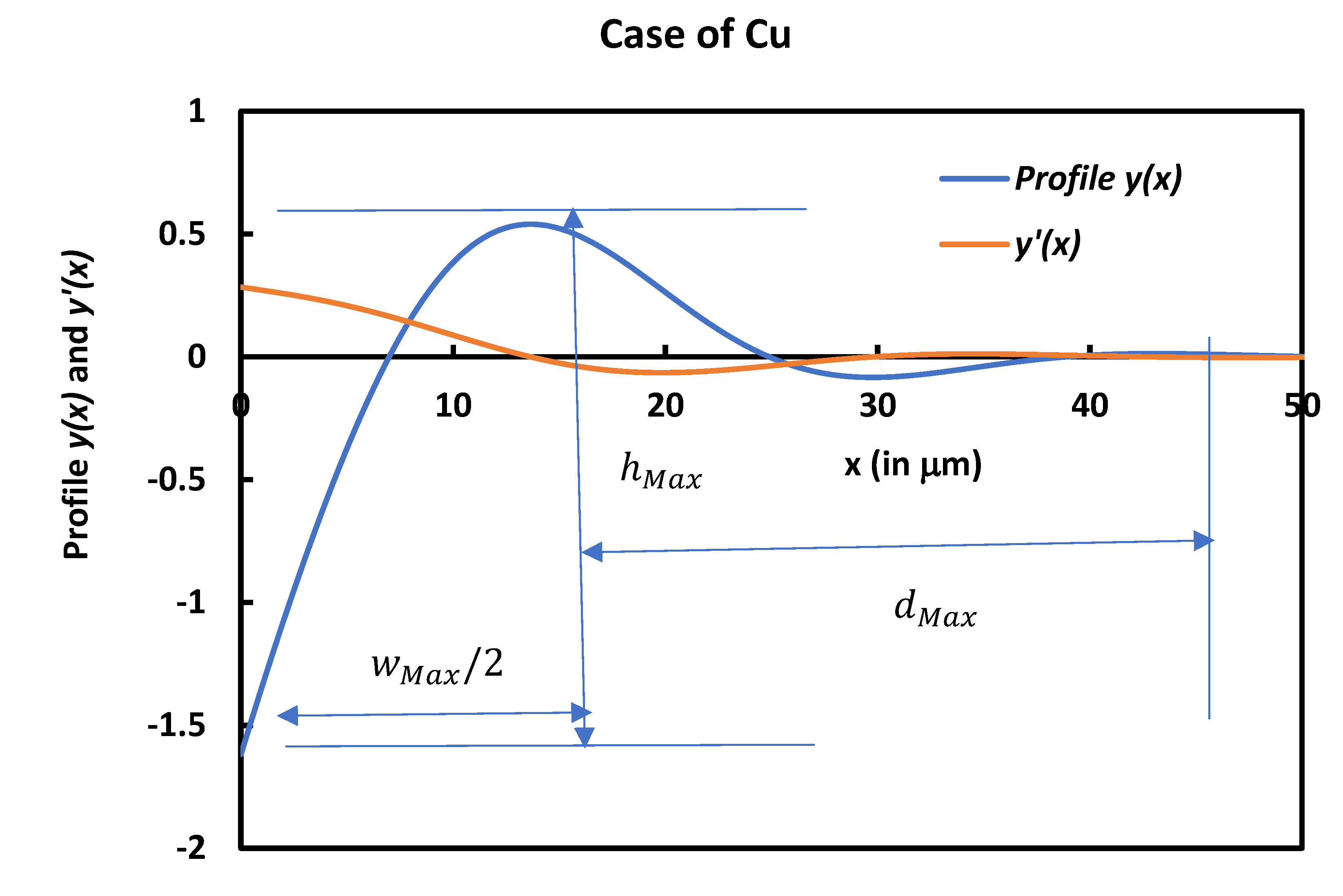
Figure 5.
Variations of the profile y(x) as a function of the distance x for different values of m corresponding to θ = 2.3° to 26.6° for copper metal.
Figure 5.
Variations of the profile y(x) as a function of the distance x for different values of m corresponding to θ = 2.3° to 26.6° for copper metal.
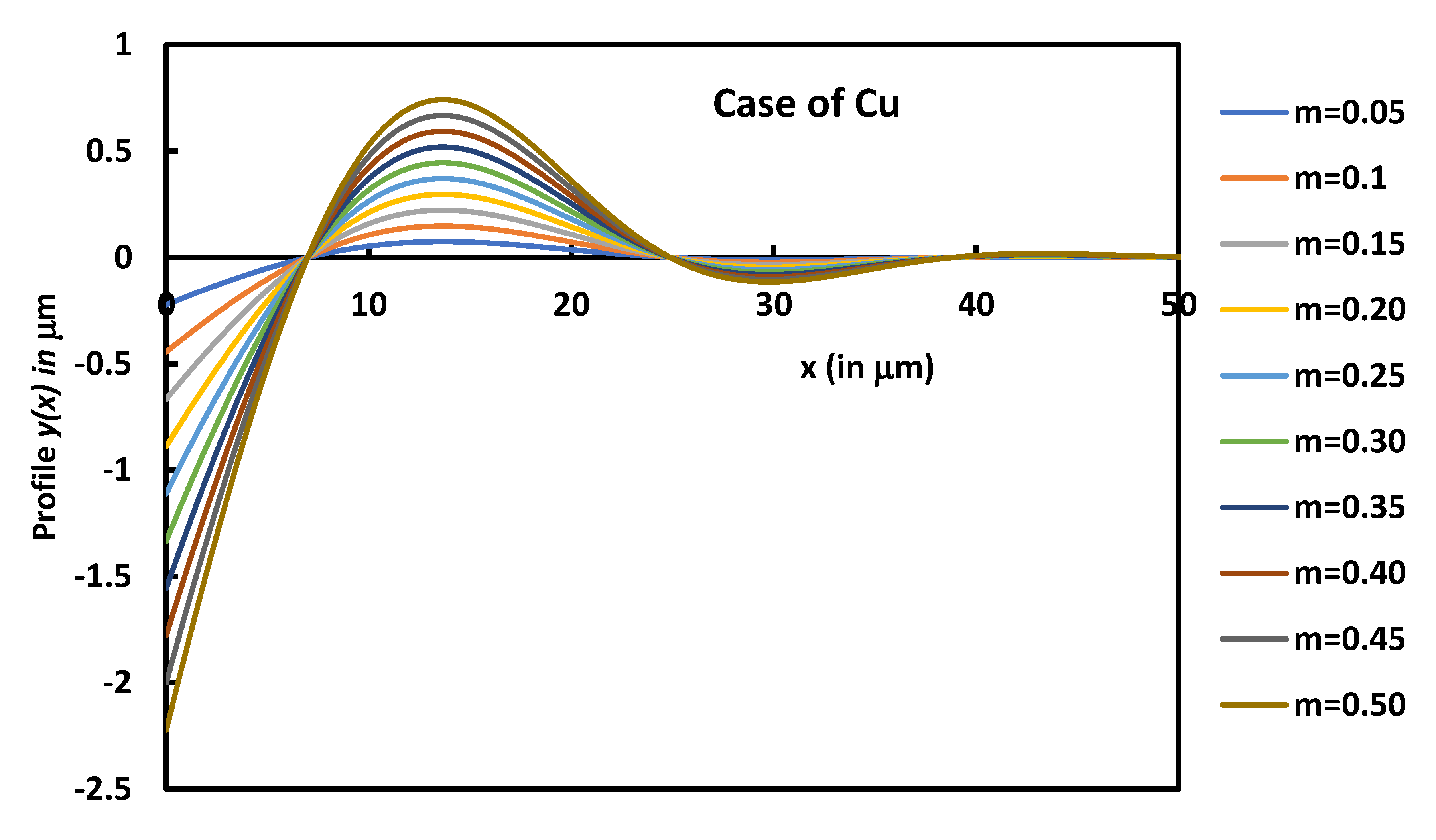
Figure 6.
Variations of the profile y(x) as a function of the distance x for the different metals at t = 24 hours.
Figure 6.
Variations of the profile y(x) as a function of the distance x for the different metals at t = 24 hours.
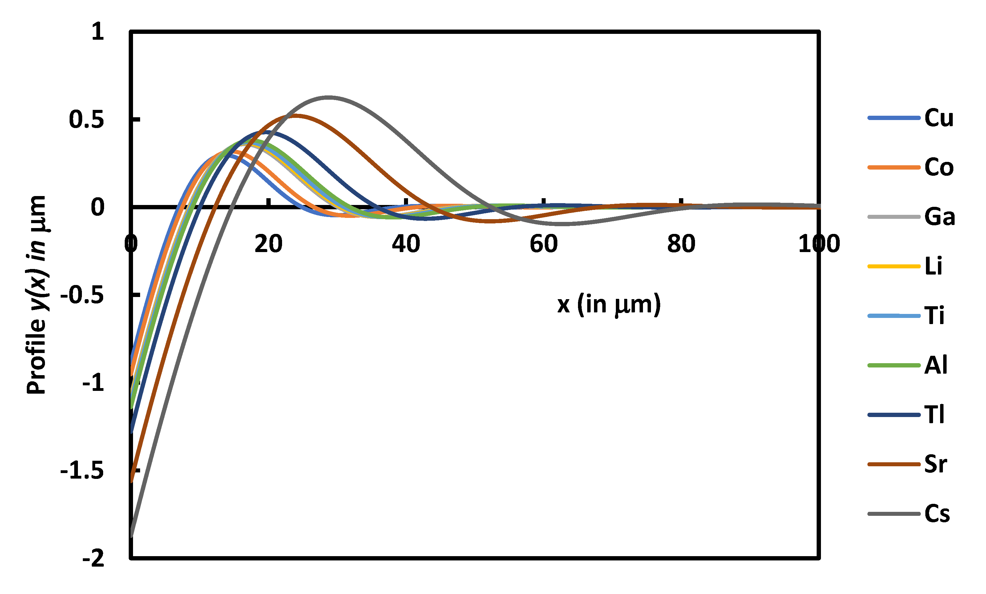

Table 1.
Values of the coordinates of Maxima and minima of the function with the
| Number N | |||||||
| 1 | 2.4 | 2.60x10⁻¹ | -1.35 | 5.22 | -4.02 x10⁻² | 3.21 | 1.22 |
| 2 | 7.62 | 6.44 x10⁻³ | -5.05 | 9.66 | -1.05 x10⁻³ | 6.86 | 4.35 |
| 3 | 11.62 | 1.70 x10⁻⁴ | -8.68 | 13.7 | -2.57 x10⁻⁵ | 10.57 | 6.78 |
| 4 | 15.26 | 4.50 x10⁻⁶ | -12.31 | 16.98 | -7.33 x10⁻⁷ | 14.13 | 9 |
| 5 | 18.62 | 1.19 x10⁻⁷ | -15.94 | 20.26 | -1.95 x10⁻⁸ | 17.76 | 11 |
| 6 | 21.82 | 3.17 x10⁻⁹ | -19.57 | 23.34 | -5.17 x10⁻¹⁰ | 21.38 | 12.89 |
| 7 | 24.82 | 8.42 x10⁻¹¹ | -23.20 | 26.3 | -1.37 x10⁻¹¹ | 25.01 | 14.69 |
| 8 | 27.74 | 2.24 x10⁻¹² | -26.83 | 29.14 | -3.64 x10⁻¹³ | 28.64 | 16.44 |
| 9 | 30.54 | 5.94 x10⁻¹⁴ | -30.45 | 31.9 | -9.67 x10⁻¹⁵ | 32.27 | 18.08 |
| 10 | 33.26 | 1.58 x10⁻¹⁵ | -34.08 | 34.58 | -2.57 x10⁻¹⁶ | 35.90 | 19.72 |
| 11 | 35.94 | 4.19 x10⁻¹⁷ | -37.71 | 37.22 | -6.84 x10⁻¹⁸ | 39.52 | 21.27 |
| 12 | 38.5 | 1.11 x10⁻¹⁸ | -41.34 | 39.78 | -1.82 x10⁻¹⁹ | 43.15 | 22.83 |
Table 2.
values of the differences between two consecutive maxima and minima.
| Number | ||||
| 1 | - | - | - | - |
| 2 | 5.22 | 3.70 | 4.44 | 3.65 |
| 3 | 4.00 | 3.63 | 4.04 | 3.71 |
| 4 | 3.64 | 3.63 | 3.28 | 3.56 |
| 5 | 3.36 | 3.63 | 3.28 | 3.63 |
| 6 | 3.20 | 3.63 | 3.08 | 3.63 |
| 7 | 3.00 | 3.63 | 2.96 | 3.63 |
| 8 | 2.92 | 3.63 | 2.84 | 3.63 |
| 9 | 2.80 | 3.63 | 2.76 | 3.63 |
| 10 | 2.72 | 3.63 | 2.68 | 3.63 |
| 11 | 2.68 | 3.63 | 2.64 | 3.63 |
| 12 | 2.56 | 3.63 | 2.56 | 3.63 |
Table 3.
Equations of interpolation of the various parameters of the groove profile.
| Parameters of the groove | Equation of interpolation | Linear regressioncoefficient |
| in (𝐵𝑡)1/4 = f(N) | = -0.0929 N2 + 4.3906N - 1.1605 | R² = 0.9991 |
| = f(N) | = 0.0012 N2 - 3.6476N + 2.2688 | R² = 1.0000 |
| or in (𝐵𝑡)1/4 | = -0.0579 N2 + 2.6546N - 0.9316 | R² = 0.9990 |
| in (𝐵𝑡)1/4= f(N) | = -0.0767 N2 + 4.0748N + 1.6466 | R² = 0.9996 |
| = f(N) | = -0.0006 N2 + 3.6352N - 0.3982 | R² = 1 |
| = -0.0102 - 0.7048 + 0.6885 | R² = 0.9998 | |
| = -0.0002 + 0.6073 - 0.2429 | R² = 1 | |
| = 0.0093+ 0.7442 - 1.0789 | R² = 1 | |
| = -0.0012 + 0.6723 - 2.1302 | R² = 0.9999 | |
| Inflexion point | = -0.0436 N2 + 2.3829N + 1.378 | R2 =0.9996 |
Table 4.
Comparison between the results of our analytical solution and those obtained by Mullins.
| Studied parameter | Results obtained by using our solution | Results obtained by Mullins |
|---|---|---|
| Approached equation of the groove profile | ||
| First zero of y | 1.22 | 1.14 |
| Coordinates of the principal maximum | (2.40; 0.260) | (2.30; 0.193) |
| Coordinates of the first inflexion point | (3.475; 0.131) | 3.43 |
| Equations of inflexion point | = -0.0436 N2 + 2.3829N + 1.378R2 =0.9996 | Not given |
| Positive inflexion point relation | = -0.0134 - 0.6214 + 0.3252R² = 0.9999 | Not given |
| Negative inflexion point relation | = 0.012 + 0.6638 - 0.6231R² = 1 | Not given |
Table 5.
Separation distance Between two consecutive maxima or minima and their ratios on the groove depth.
Table 5.
Separation distance Between two consecutive maxima or minima and their ratios on the groove depth.
| Separation distance | Equation of interpolation | |
| Between two consecutive maxima | ||
| Between two consecutive minima |
Table 6.
Values of the principal maximum, distance between the two first maxima and their ratios by using our analytical solution compared to those obtained by Mullins.
Table 6.
Values of the principal maximum, distance between the two first maxima and their ratios by using our analytical solution compared to those obtained by Mullins.
| Studied parameter | Results from our solution | Results of Mullins |
|---|---|---|
| Depth of the groove profile, |
With an error of 6.5% |
|
| Separation distance between the two first maxima |
With an error of 11.88% |
|
| Ratio |
With an error of 5.78% |
Table 7.
Coordinates of the positive and negative inflexion points and relations between coordinates.
Table 7.
Coordinates of the positive and negative inflexion points and relations between coordinates.
| Number | ||
|---|---|---|
| 1 | 3.475 | 1.310 x10⁻¹ |
| 2 | 8.295 | 3.436 x10⁻³ |
| 3 | 12.275 | 9.068 x10⁻⁵ |
| 4 | 15.855 | 2.410 x10⁻⁶ |
| 5 | 19.185 | 6.503 x10⁻⁸ |
| 6 | 22.325 | 1.744 x10⁻⁹ |
| Equation | + 0.3252 ; R² = 0.9999 | |
| Number | Abscissa of the negative inflexion point | Ordinate of the negative inflexion point |
| 1 | 6.055 | -2.109 x10⁻² |
| 2 | 10.355 | -5.568 x10⁻⁴ |
| 3 | 14.105 | -1.487 x10⁻⁵ |
| 4 | 17.545 | -4.013 x10⁻⁷ |
| 5 | 20.775 | -1.040 x10⁻⁸ |
| 6 | 23.845 | -2.823 x10⁻¹⁰ |
| Equation | - 0.6231 ; R² = 1 | |
Table 8.
Thermodynamic parameters of Au and Mg.
| Molecular mass m | |
|---|---|
| Temperature T (K) | 725.15 K |
| Surface energy γ | 1J/m2 |
| Number of molecules/m2, | |
| kT | 10-20 J |
| 10-7 m2/s | |
| Molecular volume | |
| Vapor pressure P0 of Au | |
| P0 of Mg |
Table 9.
Values of C, B and profile area of Au and Mg by using our new method compared to the values of Mullins.
Table 9.
Values of C, B and profile area of Au and Mg by using our new method compared to the values of Mullins.
| Parameter | Our results | Mullins results |
|---|---|---|
| C | ||
| B | ||
Table 10.
Values of and thermodynamic parameters of some metals, such as melting point: TMP (K), temperature of metal: T (K), vapor pressure at T: P0 (Pa), molar mass: M (g/mol), surface energy of metal: γ (J/m2) and atomic volume: ω (m3).
Table 10.
Values of and thermodynamic parameters of some metals, such as melting point: TMP (K), temperature of metal: T (K), vapor pressure at T: P0 (Pa), molar mass: M (g/mol), surface energy of metal: γ (J/m2) and atomic volume: ω (m3).
| Metal | M (g/mol) | γ (J/m2) | ω (m3) | TMP (K) | T (K) | P0 (Pa) | |
|---|---|---|---|---|---|---|---|
| Cu | 63.546 | 1.808 | 1.18 x10⁻²⁹ | 1358.2 | 2200 | 11490.38 | 1.2 x 10⁻⁵ |
| Al | 26.9815 | 1.152 | 2.32 x10⁻²⁹ | 933.5 | 2000 | 2956.96 | 1.9 x 10⁻⁵ |
| Ti | 47.867 | 2.045 | 1.77 x10⁻²⁹ | 1941.2 | 2370 | 286.35 | 2.5 x 10⁻⁴ |
| Cs | 132.905 | 0.095 | 1.18 x10⁻²⁸ | 302.96 | 530 | 425.19 | 2.0 x 10⁻⁴ |
| Li | 6.941 | 0.524 | 2.18 x10⁻²⁹ | 453.7 | 970 | 294.34 | 1.5 x 10⁻⁴ |
| Co | 58.933 | 2.536 | 1.11x10⁻²⁹ | 1768.2 | 2120 | 303.04 | 3.8 x 10⁻⁴ |
| Ga | 69.723 | 0.991 | 1.96 x10⁻²⁹ | 302.96 | 1570 | 278.52 | 4.1 x 10⁻⁴ |
| Tl | 204.383 | 0.639 | 2.86 x10⁻²⁹ | 577.2 | 1070 | 318.79 | 5.2 x 10⁻⁴ |
| Sr | 87.62 | 0.415 | 5.60 x10⁻²⁹ | 1050.2 | 1030 | 1008.65 | 6.9 x 10⁻⁵ |
Table 11.
Calculated values of evaporation C and diffusion B constants from the experimental data.
| Metal | for 24 hours | ||
|---|---|---|---|
| Co | 5.9×10⁻¹⁵ | 1.6×10⁻²⁶ | 6.1×10⁻⁶ |
| Ti | 9.6×10⁻¹⁵ | 2.9×10⁻²⁶ | 7.1×10⁻⁶ |
| Ga | 1.0×10⁻¹⁴ | 2.6×10⁻²⁶ | 6.9×10⁻⁶ |
| Li | 1.5×10⁻¹⁴ | 2.8×10⁻²⁶ | 7.0×10⁻⁶ |
| Tl | 2.9×10⁻¹⁴ | 5.3×10⁻²⁶ | 8.2×10⁻⁶ |
| Al | 1.2×10⁻¹³ | 3.4×10⁻²⁶ | 7.3×10⁻⁶ |
| Cu | 1.7×10⁻¹³ | 1.2×10⁻²⁶ | 5.7×10⁻⁶ |
| Sr | 2.4×10⁻¹³ | 1.4×10⁻²⁵ | 1.0×10⁻⁵ |
| Cs | 2.8×10⁻¹³ | 2.7×10⁻²⁵ | 1.2×10⁻⁵ |
Table 12.
Variations of the depth (in m) of the groove in the case of diffusion of different metals as a function of time.
Table 12.
Variations of the depth (in m) of the groove in the case of diffusion of different metals as a function of time.
| Metal | 1 s | 1 minute | 1 hour | 1 half-day | 1 day | 5 days | 10 days |
|---|---|---|---|---|---|---|---|
| Co | 7.4×10⁻⁸ | 2.1×10⁻⁷ | 5.7×10⁻⁷ | 1.1×10⁻⁶ | 1.3×10⁻⁶ | 1.9×10⁻⁶ | 2.3×10⁻⁶ |
| Ti | 8.6×10⁻⁸ | 2.4×10⁻⁷ | 6.7×10⁻⁷ | 1.2×10⁻⁶ | 1.5×10⁻⁶ | 2.2×10⁻⁶ | 2.6×10⁻⁶ |
| Ga | 8.4×10⁻⁸ | 2.3×10⁻⁷ | 6.5×10⁻⁷ | 1.2×10⁻⁶ | 1.4×10⁻⁶ | 2.1×10⁻⁶ | 2.6×10⁻⁶ |
| Li | 8.5×10⁻⁸ | 2.4×10⁻⁷ | 6.6×10⁻⁷ | 1.2×10⁻⁶ | 1.5×10⁻⁶ | 2.2×10⁻⁶ | 2.6×10⁻⁶ |
| Tl | 1.0×10⁻⁷ | 2.8×10⁻⁷ | 7.7×10⁻⁷ | 1.4×10⁻⁶ | 1.7×10⁻⁶ | 2.6×10⁻⁶ | 3.0×10⁻⁶ |
| Al | 8.9×10⁻⁸ | 2.5×10⁻⁷ | 6.9×10⁻⁷ | 1.3×10⁻⁶ | 1.5×10⁻⁶ | 2.3×10⁻⁶ | 2.7×10⁻⁶ |
| Cu | 6.9×10⁻⁸ | 1.9×10⁻⁷ | 5.4×10⁻⁷ | 1.0×10⁻⁶ | 1.2×10⁻⁶ | 1.8×10⁻⁶ | 2.1×10⁻⁶ |
| Sr | 1.3×10⁻⁷ | 3.5×10⁻⁷ | 9.8×10⁻⁷ | 1.8×10⁻⁶ | 2.2×10⁻⁶ | 3.2×10⁻⁶ | 3.9×10⁻⁶ |
| Cs | 1.5×10⁻⁷ | 4.2×10⁻⁷ | 1.2×10⁻⁶ | 2.2×10⁻⁶ | 2.6×10⁻⁶ | 3.8×10⁻⁶ | 4.6×10⁻⁶ |
Table 13.
Variations of the width (in m) of the groove in the case of diffusion of different metals as a function of time.
Table 13.
Variations of the width (in m) of the groove in the case of diffusion of different metals as a function of time.
| Metal | 1 s | 1 minute | 1 hour | 1 half-day | 1 day | 5 days | 10 days |
|---|---|---|---|---|---|---|---|
| Co | 1.7×10⁻⁶ | 4.8×10⁻⁶ | 1.3×10⁻⁵ | 2.5×10⁻⁵ | 2.9×10⁻⁵ | 4.4×10⁻⁵ | 5.2×10⁻⁵ |
| Ti | 2.0×10⁻⁶ | 5.5×10⁻⁶ | 1.5×10⁻⁵ | 2.9×10⁻⁵ | 3.4×10⁻⁵ | 5.1×10⁻⁵ | 6.1×10⁻⁵ |
| Ga | 1.9×10⁻⁶ | 5.4×10⁻⁶ | 1.5×10⁻⁵ | 2.8×10⁻⁵ | 3.3×10⁻⁵ | 5.0×10⁻⁵ | 5.9×10⁻⁵ |
| Li | 2.0×10⁻⁶ | 5.5×10⁻⁶ | 1.5×10⁻⁵ | 2.8×10⁻⁵ | 3.4×10⁻⁵ | 5.0×10⁻⁵ | 6.0×10⁻⁵ |
| Tl | 2.3×10⁻⁶ | 6.4×10⁻⁶ | 1.8×10⁻⁵ | 3.3×10⁻⁵ | 4.0×10⁻⁵ | 5.9×10⁻⁵ | 7.0×10⁻⁵ |
| Al | 2.1×10⁻⁶ | 5.7×10⁻⁶ | 1.6×10⁻⁵ | 3.0×10⁻⁵ | 3.5×10⁻⁵ | 5.3×10⁻⁵ | 6.3×10⁻⁵ |
| Cu | 1.6×10⁻⁶ | 4.5×10⁻⁶ | 1.2×10⁻⁵ | 2.3×10⁻⁵ | 2.7×10⁻⁵ | 4.1×10⁻⁵ | 4.9×10⁻⁵ |
| Sr | 2.9×10⁻⁶ | 8.1×10⁻⁶ | 2.3×10⁻⁵ | 4.2×10⁻⁵ | 5.0×10⁻⁵ | 7.5×10⁻⁵ | 8.9×10⁻⁵ |
| Cs | 3.5×10⁻⁶ | 9.6×10⁻⁶ | 2.7×10⁻⁵ | 5.0×10⁻⁵ | 5.9×10⁻⁵ | 8.9×10⁻⁵ | 1.1×10⁻⁴ |
Disclaimer/Publisher’s Note: The statements, opinions and data contained in all publications are solely those of the individual author(s) and contributor(s) and not of MDPI and/or the editor(s). MDPI and/or the editor(s) disclaim responsibility for any injury to people or property resulting from any ideas, methods, instructions or products referred to in the content. |
© 2023 by the authors. Licensee MDPI, Basel, Switzerland. This article is an open access article distributed under the terms and conditions of the Creative Commons Attribution (CC BY) license (http://creativecommons.org/licenses/by/4.0/).
Copyright: This open access article is published under a Creative Commons CC BY 4.0 license, which permit the free download, distribution, and reuse, provided that the author and preprint are cited in any reuse.


