Submitted:
09 August 2023
Posted:
11 August 2023
You are already at the latest version
Abstract
The refractive index of solids guages their transparency to incident light, while the energy gap determines the threshold for light absorption. This paper provides a mathematical formulation for the relationship between refractive index and energy gap. It is also established that this formulation aided in the unification of the Moss, Ravindra, and Herve-Vandamme relationships.
Keywords:
energy gap
; refractive index
; Moss
; Ravindra
; Herve-Vandamme relationships
; Wemple and DiDomenico single oscillator model
1. Introduction
Light interacts with solids through several ways, depending on the material and incident frequency under consideration. Many semiconductors are normally opaque to some higher frequencies and transparent to lower frequencies. Insulators or dielectrics are mostly transparent to visible light and metallic solids appear shiny as they reflect practically any frequency of light. The complex refractive index is adequate to assess light interaction with solids. Depending on the frequency of incident light, a material with a real refractive index closer to unity is generally transparent to that incident light, and transparency decreases with increasing refractive index. The energy gap, on the other hand, defines the threshold for light absorption in solids. In semiconductors, opacity is defined by incident photon energy surpassing the energy gap. Visible light is not absorbed by insulators or dielectrics due to their wider energy gap. Because metallic solids lack an energy gap, mobile electrons reflect incident photons, making them shine. As a result, one can simply conclude that the refractive index has an inverse relationship with the energy gap. Furthermore, the refractive index and the energy gap are two fundamental variables that play an important role in understanding electronic, optical, or optoelectronic properties in semiconductor based devices [1,2,3]. In general, a material’s refractive index is a function of frequency and doping, and various literature studies highlight the refractive index’s dependence on thickness, voids, grain boundaries, and other parameters [4,5,6]. To avoid such variations, it is best practice to consider the static refractive index determined from the time-independent electric field, and it should be noted that this article only addresses the static refractive index.
In 1950, Moss was the first to establish the inverse relationship between refractive index (n) and energy gap () [7]. This relationship was built on the broad assumption that all energy levels in a solid are scaled down by a factor of , where being the effective dielectric constant (). The photo effect process that occurs in the lattice defects found in alkali halides provides support for this claim. Such lattice defect spots behave as hydrogen-like centers where the electron behaves as an electron in an isolated atom with a bulk material-based dielectric constant. As a result, there appears to be some correlation between the scale factor and the ionization energy of the hydrogen atom. Moss observed a good relationship between the experimental data of the threshold long wavelength for photoconductive substances with the corresponding refractive index n and found that the ratio close to 77 /. Regarding the energy gap, the Moss relation becomes
The constant on the right hand side of Equation 1 is found by fitting the data and depends on the solids’ lattice structure. One of the limitations of the Moss relation is the lack of uniqueness of its constant. According to Moss, the constant for zinc blende and diamond structure lies within of 174 [8]. Based on the nature of the constant, numerous adjustments to the Moss relation are made by better fitting experimental data. Ravindra and Srivastava [9] proposed the following revised value of Moss constant,
Similarly, Reddy and Ahammed [10] altered Moss’s relationship as
Since the energy levels in a solid are highly complex and require band structure theory, all of these variations are caused by a structural restriction on the Moss relation. Second, the constant can vary amongst solids, ranging from direct to indirect interband transitions.
In 1979, Ravindra et al. [11] proposed an alternative linear empirical relation linking n with as,
where the values of the constants and , which were determined through empirical fitting, are and , respectively. After a year, the mathematical underpinnings of this linear relation were provided by Gupta and Ravindra [12], based on the Penn model [13] and Wemple-DiDomenico single oscillator model [14,15]. Their formulations made the assumption that the trajectories of the valence and conduction bands are roughly parallel to one another, at least along the symmetry axes, and that the difference between the Penn gap or the oscillatory resonance energy with the energy gap is constant. In contrast to the Moss relation, the Ravindra relation has no structural constraints. The latter relation, on the other hand, places an upper limit on the refractive index (do not predict refractive index beyond ) and provides a good approximation for the intermediate value of the energy gap (from to ) in semiconductors. One serious limitation of Ravindra relation is that it gives negative indices for .
In 1994, Herve and Vandamme [16] presented n- relationship based on the classical oscillatory theory as
where A and B are constants. The value of B is thought to reflect a constant difference between the UV resonance energy and the energy gap, which is , whereas the constant A was discovered by fitting to be , which corresponds to the hydrogen ionization energy. Except for materials (, , ), the Herve-Vandamme relation provides a good fit to the related experimental data for the majority of materials.
Since 1950, multiple empirical relations have been proposed by various researchers to account for both the structural and refractive index restrictions of the Moss and Ravindra relations. There is still a lack of a robust theoretical foundation in this discipline. Finkenrath [17] used the band theory in 1988 to theoretically develop the Moss-like relation and the Ravindra relation.
This paper’s main goal is to establish a single mathematical framework for the formulation of Moss, Ravindra, and Herve-Vandamme relationships. Since these relationships are empirical, the physical knowledge of the fitting parameters (constants) is limited. Additionally, this work aims to provide light on these fitting parameters.
2. Mathematical formulation
This model suggests an arbitrary function , which is expressed as a power series of as,
where, p is a number and it will be shown here that for a suitable value of p, the series (6) converges to
iff
Proof.
Starting from
and substituting the value of from equation (8) yields,
evaluating the summation and rearranging yields,
The bracketed terms is a well-known binomial series, which converges to an equation (7) whenever
Conversely, let us define a function
then, the value of g and its derivatives at zero can be found as,
This allows to express and as,
Comparing equation (22) with equation (6) yields,
Furthermore, the convergence condition yields the following two possibilities:
(i) positive p and ⇒
(ii) negative p and ⇒
This completes the proof. Here, it is not disclosed about and K. In the next section, the search for the physical meaning of , K and p is implemented. □
3. , K and p
The well-known Sellmeier dispersion model [18] is,
is the empirical parameter that corresponds to the strength of undamped Lorentz oscillators. Using generalized Lorentz oscillator model [19],
where is the plasma frequency and is the oscillator strength associated with transitions at frequency . Wemple and DiDomenico (WD) [14,15] suggested a single oscillator model that could be considered dominant among other oscillators and proposed,
F being the overall oscillator strength and is given as,
is the dominant oscillator frequency. Using the moment of the optical spectra and Kramers-Kronig relation [14,15], WD found that , where the parameters and are the oscillator resonance energy and dispersion energy, respectively. In terms of Sellmeier model this can also be written for dominant oscillator as , where is the dominant oscillatory strength instead of the electric-dipole oscillator strength associated with transitions at a specific frequency. Thus, the well known WD model is,
If K is the separation of the dominant oscillator energy from the minimum energy gap then under the condition the WD model can be written as,
Equation (29) satisfies the requirement shown by Equation (3), and therefore enables us to compare with Equation (11), which yields,
where,
Hence, the required model for the refractive index n can be written as,
and based on the convergence condition (i),
In most semiconductors, the refractive index’s dependence on the energy gap is mostly governed by UV oscillator energy and thus it is plausible to consider K usually exceeds . Furthermore, if then K might be expressed as and thus, from the band structure point of view p as unity is more preferable at least for direct band gap materials, which has also been justified by the WD model. Moreover, one can clearly notice that is a unitless quantity and K has a unit of energy. In the next section, it will be shown that Equation (33) is the basis equation that can connect the Moss, Ravindra, and Herve-Vandamme relations and offer insight on the physical understanding of the constants used in these relations.
4. Results
4.1. Moss Relation
By squaring Equation (33) and simplifying one can easily get that,
One can estimate Moss constant from the WD’s constant-conductivity dielectric model [14,15], which approximate the ratio to as,
where b is a coefficient with a value of for covalent solids and for ionic solids. Equation (35) allows us to write,
The term , therefore, has a value for covalent solids and for ionic solids. This suggests to write the Moss relation as,
The WD’s constant-conductivity dielectric model assumes the ratio , and in many solids, this ratio roughly ranges from to , which might cause slight changes in the Moss constant. Table 1 highlights the calculated values of Moss constant for different materials.

Table 1.
The data in columns 3, and 4 are from sources [14,15] and rest are calculated. Columns 5, 6, and 7 show the computed Ravindra, Herve-Vandamme, and Moss constants, respectively. The data in the second and last columns are taken from source [20].
| : ; | : A; B | ||||||
|---|---|---|---|---|---|---|---|
| C | 5.4 | 10.9 | 49.7 | 3.32; 0.30 | 23.27; 5.5 | 166.91 | 2.35 |
| 1.1 | 4.0 | 44.4 | 4.08;0.70 | 13.32;2.9 | 161.06 | 3.46 | |
| 0.67 | 2.7 | 41.0 | 4.64;1.14 | 10.52;2.03 | 175.51 | 4.0 | |
| 1.43 | 3.55 | 33.5 | 4.18;0.98 | 10.90;2.12 | 155.76 | 3.3 | |
| 2.24 | 4.46 | 36.0 | 4.27;0.96 | 12.67;2.22 | 184.34 | 2.9 | |
| 0.18 | 2.3 | 35.0 | 4.19;0.99 | 8.97;2.12 | 47.34 | 3.95 | |
| 2.45 | 5.6 | 34.9 | 3.58;0.57 | 13.98;3.15 | 128.14 | 2.75 | |
| 2.18 | 4.7 | 33.7 | 3.90;0.77 | 12.58;2.52 | 145.52 | 3.0 | |
| 12.50 | 17.1 | 14.9 | 2.63;0.28 | 15.96;4.6 | 43.77 | 1.39 | |
| 10.5 | 15 | 11.3 | 2.42;0.27 | 13.01;4.5 | 32.28 | 1.33 | |
| 10.3 | 14.8 | 12.3 | 2.45;0.27 | 13.50;4.5 | 34.53 | 1.36 | |
| 8.9 | 10.3 | 13.6 | 4.13;1.47 | 11.83;1.40 | 47.92 | 1.54 | |
| 8.5 | 10.5 | 12.3 | 3.38;0.84 | 11.96;2 | 40.08 | 1.49 | |
| 8.3 | 10.4 | 12.2 | 3.28;0.78 | 11.26;2.1 | 39.19 | 1.49 | |
| 8 | 10.6 | 14 | 3.97;0.59 | 12.18;2.60 | 43.09 | 1.61 | |
| 7.2 | 9.1 | 12.1 | 3.34;0.88 | 10.54;1.90 | 39.08 | 1.55 | |
| 6.17 | 7.7 | 12.8 | 3.66;1.19 | 9.92;1.53 | 43.73 | 1.67 | |
| 5.8 | 7.7 | 12.1 | 3.23;0.85 | 9.65;1.90 | 38.35 | 1.64 | |
| 8.0 | 10.6 | 17.1 | 3.26;0.63 | 13.46;2.6 | 54.63 | 1.61 | |
| 7.0 | 9.4 | 17 | 3.32;0.69 | 12.64;2.40 | 55.21 | 1.67 | |
| 6.3 | 7.5 | 15.2 | 4.35;1.81 | 10.67;1.20 | 57.71 | 1.82 | |
| 2.11 | 5.8 | 20.6 | 2.67;0.36 | 10.93;3.69 | 43.71 | 2.08 | |
| 2.68 | 5.3 | 21.7 | 3.21;0.61 | 10.72;2.62 | 69.55 | 2.25 | |
| 11.8 | 15.7 | 15.9 | 2.84;0.36 | 15.80;3.90 | 47.80 | 1.43 | |
| 10.5 | 13.8 | 15.9 | 3.0;0.45 | 14.81;3.3 | 48.63 | 1.47 | |
| 5.13 | 7.4 | 22 | 3.6;0.80 | 12.76;2.27 | 80.97 | 1.9 | |
| 3.31 | 7.3 | 18.1 | 2.52;0.31 | 11.49;3.99 | 40.07 | 2.19 | |
| 3.7 | 6.4 | 17.1 | 2.95;0.55 | 10.46;2.70 | 49.88 | 1.92 | |
| 2.4 | 4.9 | 20.4 | 3.18;0.64 | 9.99;2.5 | 63.98 | 2.38 | |
| 1.74 | 4.0 | 20.6 | 3.29;0.73 | 9.08;2.26 | 65.81 | 2.49 | |
| 3.54 | 6.15 | 25.2 | 3.46;0.66 | 12.45;2.61 | 91.98 | 2.27 | |
| 7.8 | 11.3 | 22.0 | 3.08;0.44 | 15.77;3.5 | 67.74 | 1.62 | |
| 6.26 | 9.9 | 22.6 | 2.98;0.41 | 14.96;3.64 | 67.46 | 1.39 | |
| 6.96 | 13.4 | 27.5 | 2.52;0.195 | 19.19;6.44 | 64.84 | 1.63 | |
| 6.5 | 11.1 | 25.4 | 2.82;0.31 | 16.80;4.60 | 70.28 | 1.71 | |
| 3.7 | 6.24 | 23.2 | 3.40;0.67 | 12.03;2.54 | 82.36 | 2.2 | |
| 4.10 | 5.68 | 23.7 | 4.31;1.36 | 11.60;1.58 | 109.70 | 2.38 | |
| 4.12 | 5.57 | 23.3 | 4.46;1.54 | 11.40;1.45 | 110.68 | 2.4 | |
| 3.70 | 6.50 | 23.7 | 3.28;0.58 | 12.41;2.8 | 79.87 | 2.2 | |
| 4.7 | 7.49 | 26.1 | 3.47;0.62 | 13.98;2.80 | 94.53 | 2.18 | |
| 4.0 | 6.65 | 25.9 | 3.50;0.66 | 13.12;2.65 | 95.83 | 2.34 | |
| 3.2 | 5.24 | 25.7 | 3.89;0.95 | 11.60;2.04 | 111.56 | 2.72 | |
| 7.80 | 12.1 | 23.3 | 2.87;0.33 | 16.80;4.3 | 66.76 | 1.52 | |
| 4.20 | 9.15 | 23.3 | 2.56;0.25 | 14.60;4.95 | 52.82 | 1.81 | |
| 3.56 | 7.46 | 26.0 | 2.93;0.37 | 13.93;3.9 | 71.62 | 2.1 | |
| 4.50 | 8.26 | 23.0 | 2.88;0.38 | 13.78;3.76 | 64.45 | 1.90 | |
| 3.2 | 5.40 | 22.60 | 3.56;0.81 | 11.04;2.2 | 86.03 | 2.2 | |
| 4.16 | 8.60 | 21.30 | 2.60;0.29 | 13.53;4.44 | 50.28 | 1.85 | |
| 9.3 | 13.6 | 18.3 | 2.72;0.32 | 15.77;4.30 | 51.16 | 1.46 | |
| 3.54 | 6.36 | 26.1 | 3.39;0.60 | 12.88;2.82 | 92.21 | 2.27 | |
| 2.58 | 5.54 | 27.0 | 3.31;0.56 | 12.23;2.96 | 89.0 | 2.43 | |
| 2.26 | 4.34 | 27.0 | 3.88;0.93 | 10.82;2.08 | 117.85 | 2.70 | |
| 1.58 | 4.13 | 25.7 | 3.42;0.67 | 10.30;2.55 | 82.42 | 2.7 | |
| 0.286 | 3.5 | 55.33 | 4.28;0.66 | 13.91;3.21 | 80.55 | 4.1 | |
| 0.165 | 3.0 | 66.12 | 4.94;0.87 | 14.08;2.83 | 87.58 | 4.8 | |
| 0.190 | 2.2 | 66.80 | 5.86;1.46 | 12.12;2.01 | 186.90 | 5.6 |
4.2. Ravindra Relation
As Ravindra relation is a linear relation, it is produced by expanding Equation (33) and approximating it by just taking into account the linear parts. This results,
The similar linear relationship was derived by Gupta and Ravindra [12], who found that the values of (≈) and (≈) by empirical fittings. Table 1 highlights the calculated values of and for different materials.
4.3. Herve-Vandamme Relation
Herve and Vandamme made the assumption that , or the constant difference of “−" had a B parameter with a value of eV. Replacing K with B and performing a simple computation of Equation (33) yields,
This shows that . Conversely, beginning with produces the expression,
This eventually leads to,
Using empirical fitting of experimental data, they computed A to be and regarded it as the ionization energy of a Hydrogen atom. Table 1 highlights the calculated values of A and B for different materials.
5. Discussion
5.1. Empirical fitting constants
So far, it has been shown that the empirical fitting constants associated with the Moss, Ravindra, and Herve-Vandamme relationships are connected to and K, which are functions of and . These constants are thus specific to each material, and their numerical values were previously determined through empirical fitting. Table 1 highlights the computed values of these constants for different materials. Originally, the Ravindra constants and were estimated to be and , respectively. Moss utilized the same original value of as and computed K to be , which is quite unrealistic, and so proposed new values of and of and , respectively [21]. In contrast to Moss, this study (Equation 38) calculates to be and K to be using the same original constants and . Later on Ravindra et. al. [22] proposed more updated values of and to be and . With the help of Ravindra two constants, the single Moss constant can also be predicted using Equation 37. The predicted values of Moss constant using original and is , Moss estimated and is and Ravindra later updated values of and is . The Herve-Vandamme relation can also be used to predict the lowest bound of the Moss constant. As and so . Since ; this implies . Figure 1 shows the values of refractive indices of various materials calculated using Moss, Ravindra, and Herve-Vandamme relationships as well as with Equation 33, and compared with their respective experimental values.
According to Moss, the relationship between refractive index and energy gap must be the result of a close relationship between the energy gap and the UV absorption peak, with being one of the simplest assumptions [21]. This notion is directly used in the Herve-Vandamme relation, which assumes that the difference between the UV resonance energy and the energy gap is constant and assigns it a value of [16], whereas Ravindra relation implicitly assigns it a value of . Unlike the Moss relation, the presence of two constants in Ravindra and Herve-Vandamme relations is most likely due to one of the constants explicitly or implicitly representing this constant difference. Moreover, this study also demonstrates that the WD model directly leads to this simplest assumption of , which is sufficient to integrate the Moss, Ravindra, and Herve-Vandamme relations. However, the true nature of the refractive index dependence between the energy gap and oscillator resonance energy remains hidden. In other words, the WD model directly leads us to assume p as unity, but whether is true value or not is still unknown.
5.2. Convergence criterion
The convergence criteria that leads to Equation 33 is . In order to satisfy the requirement , must be more than twice that of (), which in turn satisfy the requirement . Based on this criteria, one can claim that the Ravindra relation should deviate when and Herve-Vandamme relation should deviate when . This claim is somehow true for Ravindra relation but not true for Herve-Vandamme relation. Similarly for Moss relation, it appears that the denominator of the right hand term in Equation 34 is quite independent of the condition . Because if then , and if then , leaving the term unchanged, resulting the Moss constant independent of the condition. Moreover, there are materials such as , , (one can find from Table 1) where the convergence criteria is violated but the indices predicted by Equation 33 is close to their respective experimental values. This contradiction implies that n should fall exponentially on until the ratio reaches unity, and then n should be roughly constant with . This means that for two or more materials having similar and have similar refractive indices. As a result, the variation of n with should be of an exponentially decreasing character, with asymptotes at .
5.3. Exceptional materials
Moss stated in his work [21] that materials such as , , and have almost the same indices despite vastly different energy gaps. Moss, Ravindra, and Herve-Vandamme relationships also vary significantly in IV-VI materials such as , , and despite these materials satisfy [9,16,21]. These remarkable materials are infrared materials, and the unique constant/constants generated by empirical fitting of distinct materials diverge substantially for such low gap materials. As previously demonstrated, the constants are a function of and , and the variation in the refractive index is due to the combined action of or , and . The refractive indices of these materials are shown in Table 2 and are well predicted by Equation 33.
6. Conclusions
In conclusion, using the WD model, this paper formulates an accurate equation relating n- as , where and K can be found for each material based on their respective and . It has been demonstrated that this equation can accurately describe all types of materials (from low energy gaps to high energy gaps). Furthermore, this formulation is enough for integrating the Moss, Ravindra, and Herve-Vandamme relations and comprehending their empirical fitting constants.
Funding
The author declare that they have no known competing financial interests or personal relationships that could have appeared to influence the work reported in this paper.
Data Availability Statement
The data presented in this study are available on request from the corresponding author.
Acknowledgments
I would like to remember Prof. N.M. Ravindra of New Jersey Institute of Technology, for his outstanding work and contributions in the field of semiconductors. I have had the opportunity to work with him during my Ph.D. This paper is dedicated to him.
Conflicts of Interest
The author declare no conflict of interest.
References
- Ou, Q.; Bao, X.; Zhang, Y.; Shao, H.; Xing, G.; Li, X.; Shao, L.; Bao, Q. Band structure engineering in metal halide perovskite nanostructures for optoelectronic applications. Nano Materials Science 2019, 1, 268–287. [Google Scholar] [CrossRef]
- Geng, T.; Ma, Z.; Chen, Y.; Cao, Y.; Lv, P.; Li, N.; Xiao, G. Bandgap engineering in two-dimensional halide perovskite Cs 3 Sb 2 I 9 nanocrystals under pressure. Nanoscale 2020, 12, 1425–1431. [Google Scholar] [CrossRef] [PubMed]
- Wu, M.J.; Kuo, C.C.; Jhuang, L.S.; Chen, P.H.; Lai, Y.F.; Chen, F.C. Bandgap engineering enhances the performance of mixed-cation perovskite materials for indoor photovoltaic applications. Advanced Energy Materials 2019, 9, 1901863. [Google Scholar] [CrossRef]
- Nenkov, M.R.; Pencheva, T.G. Determination of thin film refractive index and thickness by means of film phase thickness. Central European Journal of Physics 2008, 6, 332–343. [Google Scholar] [CrossRef]
- Ono, M.; Aoyama, S.; Fujinami, M.; Ito, S. Significant suppression of Rayleigh scattering loss in silica glass formed by the compression of its melted phase. Optics Express 2018, 26, 7942–7948. [Google Scholar] [CrossRef] [PubMed]
- Ong, H.; Dai, J.; Li, A.; Du, G.; Chang, R.; Ho, S. Effect of a microstructure on the formation of self-assembled laser cavities in polycrystalline ZnO. Journal of Applied Physics 2001, 90, 1663–1665. [Google Scholar] [CrossRef]
- Moss, T.S. A Relationship between the Refractive Index and the Infra-Red Threshold of Sensitivity for Photoconductors. Proceedings of the Physical Society. Section B 1950, 63, 167. [Google Scholar] [CrossRef]
- Moss, T.S. Photoconductivity in the Elements. Proceedings of the Physical Society. Section A 1951, 64, 590. [Google Scholar] [CrossRef]
- Ravindra, N.; Srivastava, V. Variation of refractive index with energy gap in semiconductors. Infrared Physics 1979, 19, 603–604. [Google Scholar] [CrossRef]
- Reddy, R.; Nazeer Ahammed, Y. A study on the Moss relation. Infrared Physics & Technology 1995, 36, 825–830. [Google Scholar] [CrossRef]
- Ravindra, N.; Auluck, S.; Srivastava, V. On the Penn Gap in Semiconductors. physica status solidi (b) 1979, 93, K155–K160. [Google Scholar] [CrossRef]
- Gupta, V.; Ravindra, N. Comments on the Moss Formula. physica status solidi (b) 1980, 100, 715–719. [Google Scholar] [CrossRef]
- Penn, D.R. Wave-Number-Dependent Dielectric Function of Semiconductors. Phys. Rev. 1962, 128, 2093–2097. [Google Scholar] [CrossRef]
- Wemple, S.; DiDomenico Jr, M. Behavior of the electronic dielectric constant in covalent and ionic materials. Physical Review B 1971, 3, 1338. [Google Scholar] [CrossRef]
- Wemple, S.H.; DiDomenico, M. Optical Dispersion and the Structure of Solids. Phys. Rev. Lett. 1969, 23, 1156–1160. [Google Scholar] [CrossRef]
- Hervé, P.; Vandamme, L. General relation between refractive index and energy gap in semiconductors. Infrared physics & technology 1994, 35, 609–615. [Google Scholar]
- Finkenrath, H. The Moss rule and the influence of doping on the optical dielectric constant of semiconductors—I. Infrared Physics 1988, 28, 327–332. [Google Scholar] [CrossRef]
- Sellmeier. Zur Erklärung der abnormen Farbenfolge im Spectrum einiger Substanzen. Annalen der Physik, 219, 272–282.
- Levi, A.F.J. The Lorentz oscillator model. In Essential Classical Mechanics for Device Physics; 2053-2571, Morgan & Claypool Publishers, 2016; pp. 5–1 to 5–21. [CrossRef]
- Gomaa, H.M.; Yahia, I.; Zahran, H. Correlation between the static refractive index and the optical bandgap: Review and new empirical approach. Physica B: Condensed Matter 2021, 620, 413246. [Google Scholar] [CrossRef]
- Moss, T.S. Relations between the Refractive Index and Energy Gap of Semiconductors. physica status solidi (b) 1985, 131, 415–427. [Google Scholar] [CrossRef]
- Ravindra, N.; Ganapathy, P.; Choi, J. Energy gap–refractive index relations in semiconductors – An overview. Infrared Physics & Technology 2007, 50, 21–29. [Google Scholar] [CrossRef]
Figure 1.
Calculated refractive indices in comparison to experimental values .
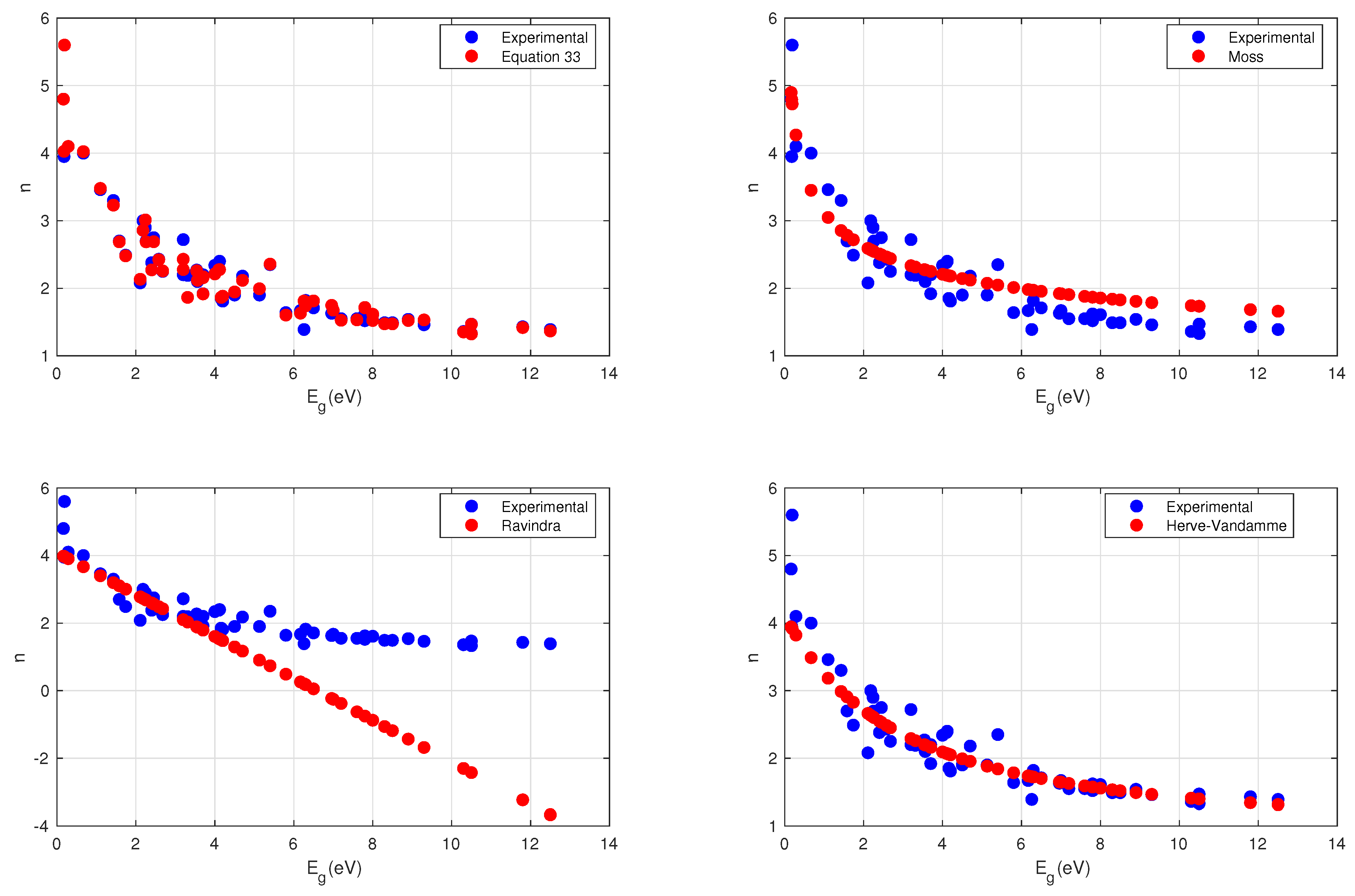
Table 2.
Computed values of refractive indices of different materials.
| (n) | 33 (n) | |||||
|---|---|---|---|---|---|---|
| 0.67 | 3.45 | 3.66 | 3.48 | 4.02 | 4.0 | |
| 0.18 | 4.79 | 3.97 | 3.93 | 4.02 | 3.95 | |
| 0.286 | 4.27 | 3.90 | 3.94 | 4.09 | 4.1 | |
| 0.165 | 4.89 | 3.98 | 3.94 | 4.79 | 4.8 | |
| 0.190 | 4.73 | 3.96 | 3.92 | 5.51 | 5.6 |
Disclaimer/Publisher’s Note: The statements, opinions and data contained in all publications are solely those of the individual author(s) and contributor(s) and not of MDPI and/or the editor(s). MDPI and/or the editor(s) disclaim responsibility for any injury to people or property resulting from any ideas, methods, instructions or products referred to in the content. |
© 2023 by the authors. Licensee MDPI, Basel, Switzerland. This article is an open access article distributed under the terms and conditions of the Creative Commons Attribution (CC BY) license (http://creativecommons.org/licenses/by/4.0/).
Copyright: This open access article is published under a Creative Commons CC BY 4.0 license, which permit the free download, distribution, and reuse, provided that the author and preprint are cited in any reuse.


