Submitted:
08 August 2023
Posted:
10 August 2023
You are already at the latest version
Abstract
The application of deep learning in the detection of Synthetic Aperture Radar (SAR) targets has been primarily limited to large objects such as ships and airplanes, with much less popularity in detecting SAR vehicles. The complexities of SAR imaging make it difficult to distinguish small vehicles from the background clutter, creating a barrier to data interpretation and the development of Automatic Target Recognition (ATR) in SAR vehicles. The scarcity of datasets has inhibited progress in SAR vehicle detection in the data-driven era. To address this, we introduce a new synthetic dataset called Mix MSTAR, which mixes target chips and clutter backgrounds with original radar data at the pixel level. Mix MSTAR contains 5,392 objects of 20 fine-grained categories in 100 high-resolution images, predominantly 1478x1784 pixels. The dataset includes various landscapes such as woods, grasslands, urban buildings, lakes, and tightly arranged vehicles, each labeled with Oriented Bounding Box (OBB). Notably, Mix MSTAR presents fine-grained object detection challenges by using the Extended Operating Condition (EOC) as a basis for dividing the dataset. Furthermore, we evaluate 9 benchmark rotated detectors on Mix MSTAR and demonstrate the fidelity and effectiveness of the synthetic dataset. To the best of our knowledge, Mix MSTAR represents the first public multi-class SAR vehicle dataset designed for rotated object detection in large-scale scenes with complex background. Mix MSTAR is available at: https://github.com/TheGreatTreatsby/Mix-MSTAR-mmrotate.
Keywords:
SAR vehicle detection
; rotated object detection
; Synthetic dataset
; Mix MSTAR
; deep learning
1. Introduction
Thanks to its unique advantages, such as all-time, all-weather, high-resolution, and long-range detection, SAR has been widely used in various fields, such as land analysis and target detection. Vehicle detection in SAR-ATR is of great significance in urban traffic, hotspot target focusing and other aspects.
In recent years, with the development of artificial intelligence, deep learning-based object detection algorithms [1,2] have dominated the field with their powerful capabilities in automatic feature extraction. Deep learning is a subject with data hunger. Historical experience has shown that big data is an important driver for the flourishing development of deep learning technology in various fields. With the rapid development of aerospace and sensor technology, an increasing number of high-resolution remote sensing images can be obtained. In the remote sensing field, visible light object detection has experienced vigorous development after the release of the DOTA[3]. As the first publicly available SAR ship dataset, the introduction of the SSDD [4] has directly promoted the application of deep learning in SAR object detection and has led to the emergence of more SAR ship datasets [5,6,7,8,9], which is still one of the detection benchmark and exhibits strong vitality to this day.
However, due to the imaging mechanism of SAR images being distinct from visible light, its interpretation is unintuitive for the human eye. Ground clutter and scattering caused by object corner points can seriously interfere with human interpretation. This leads to the fact that the detection objects of the current SAR datasets are mainly large targets such as ships and planes in relatively pure backgrounds. In contrast, SAR datasets for vehicles are very rare. The community has long relied on the Moving and Stationary Target Acquisition and Recognition (MSTAR) [10] released by the Sandia National Laboratory in the last century. However, the vehicle images in MSTAR are also separated from large-scene images and appear in the form of small patches. Due to the lack of complex background, it is only suitable for classification tasks, and its classification accuracy has reached more than 99%. Up to now, in the SAR-ATR field, MSTAR has been more widely used in few-shot learning and semi-supervised learning [11,12]. Meanwhile, the volume of the SAR dataset owning vehicle images with large scenes is quite small. The reason for this is that the small area of the vehicle requires higher resolution for SAR-ATR than aircrafts and ships, which leads to higher data acquisition costs. Moreover, vehicles exist in more complex clutter backgrounds, which increases the difficulty of manual interpretation and reduces the accuracy of target annotation. Table 1 detailed information of existing public SAR vehicle datasets with large scenes. Unfortunately, in these datasets, there is no official localization annotation that can be obtained, so manual identification of annotations is required. Due to strong noise interference, the FARAD X BAND [13]and FARAD KA BAND [14] make it too difficult for humans to identify the position of vehicles, so the annotations cannot meet the accuracy requirements. The Spotlight SAR [15] has only a very small number of vehicles, and pairs of pictures were taken at different time periods at the same location. The Mini SAR [16] includes more vehicles, but it only contains 20 pictures, and it has the same problem of Spotlight SAR in duplicate scenes. The subsequent experiments proved that the small size of Mini SAR caused a large standard error of the results. These reasons make the above datasets difficult to become a reliable benchmark for SAR-ATR algorithms. In addition, there is the GOTCHA [17], which contains vehicles and large scenes, but it is a fully polarized circular SAR dataset that is significantly different from the commonly used single polarized linear SAR. It only contains one scene and is mainly used for the classification of calibrated vehicles in the SAR-ATR field. The size of GOTCHA is difficult to meet the requirements of object detection, so it is not included in the table here for comparison.
In view of the scarcity of vehicle datasets in the SAR-ATR field, people have conducted a series of data generation work around MSTAR, which can be mainly divided into the following three methods. The first method is based on generative adversarial nets (GANs) [18]. The generating network transforms the input noise into generative images that can deceive discriminative networks by fitting the distribution of real images. In theory, GANs [19,20,21] can generate an infinite number of generative images (See Figure 1a), thereby solving the problem of scarce real samples. However, unlike optical images, SAR imaging is strictly based on radar scattering mechanisms, and the black box properties of neural networks cannot prove that the generative samples comply with SAR imaging mechanisms. Moreover, due to the limitations of real samples, it is difficult to generate large-scene images. The second method is based on computer aided design (CAD) 3D modeling and electromagnetic calculation simulation [22,23,24,25]. Among them, the SAMPLE [25] dataset released by Lewis et al. from the same institution of MSTAR, and it has advantages in model errors, as shown in Figure 1b. The advantage of this method is that the imaging of synthetic samples is based on physical mechanisms, and the imaging under different conditions can be easily obtained by changing the simulation environment parameters. Compared with the original images, the simulation images can also remove the correlation between the targets and the background by setting random background noise, which prevents overfitting of the detection model. However, both of these methods have background limitations and it is currently difficult to simulate vehicles located in complex large-scale backgrounds. The third method is background transfer [26,27,28]. Chen et al. believe that since the acquisition conditions of the chip image (Chip for short) and the clutter image (Clutter for short) in MSTAR are similar, Chips can be embedded in Clutters to generate vehicle images with large scenes , as shown in Figure 1c. Like the first method, the synthetic images cannot strictly comply with SAR imaging mechanisms, and the current use of such methods directly paste Chips with their backgrounds onto Clutters, which looks quite abrupt visually and maintaining an association between the target and the background.
To generate large-scale SAR images with complex backgrounds, we constructed the Mix MSTAR using improved a background transfer method. Unlike the previous works, we overcame the abrupt visual appearance of synthetic images and demonstrated the fidelity and effectiveness of synthetic data. Our key contributions are as follows:
- We improved the method of background transfer and generated realistic synthetic data by linearly fusing vehicle masks in Chips and Clutters, resulting in the fusion of 20 types of vehicles (5,392 in total) into 100 large background images. The dataset adopts rotation bounding box annotation and includes one Standard Operating Condition (SOC) and two EOCs partitioning strategies, making it a challenging and diverse dataset.
- Based on the Mix MSTAR, we evaluated 9 benchmark models for general remote sensing object detection and analyzed their strengths and weaknesses for SAR-ATR.
- To address potential artificial traces and data variance in synthetic images, we designed two experiments to demonstrate the fidelity and effectiveness of Mix MSTAR in SAR image features, demonstrating that Mix MSTAR can serve as a benchmark dataset for evaluating deep learning-based SAR-ATR algorithms.
The remaining article is composed of 4 sections. Section 2 presents detailed methodology employed to construct the synthetic dataset, as well as extensive analysis of the dataset itself. In Section 3, we introduce and evaluate nine rotate object detectors using the synthetic dataset as the benchmark. Sequently, a comprehensive analysis of the results is conducted. Section 4 focuses specifically on the analysis and validation of two vital problems related the dataset, namely, artificial traces and data variance. Moreover, we provide an outlook on potential future of the synthetic dataset. Section 5 concludes our work.
2. Materials and Methods
2.1. Preliminary Feasibility Assessment
We first evaluated the feasibility of merging Clutters and Chips. Since the sensor's depression was 15° when collecting Clutters, we chose Chips with the same depression as the target images. As shown in Table 2, both Clutters and Chips use the same STARLOS sensor based on airborne platform, and maintain consistency in terms of radar center frequency, bandwidth, polarization and depression. Although the radar mode is in different, the final imaging resolution and pixel spacing are the same. Therefore, we assume that if the working parameters of Clutters are used for imaging vehicles, the visual effect will be approximately the same as that on Chips. So, it is feasible to transfer the vehicles in Chips to the Clutters’ backgrounds, and the final effect is in line with the human observation mechanism. Of course, we must acknowledge that due to the differences in the operating modes, the two have significant differences in the radar raw data (especially phase). This means that synthetic data generated by background transfer cannot strictly conform to the scattering mechanism of the radar. However, what we pursue is the consistency between synthetic data and real data in terms of 8-bit image features, which is crucial for current deep learning models based on image feature extraction in the computer vision field.
Unlike previous attempts that involve crude background transfers, Mix MSTAR aims to be a visually realistic synthetic dataset. To achieve this goal, we conducted extensive research into domain transfer and imaging algorithms to harmoniously blend two different radar data and developed a paradigm for creating synthetic datasets, as shown in Figure 2. Next, we will describe in detail the process of constructing the dataset.
2.2. Mask Extraction
In order to make vehicles fit seamlessly into the Clutters’ backgrounds, we used labelme [29] to mask the outlines of the vehicles on Chips. Since the shadow in radar blind area is also the important feature of SAR targets, the shadow of the vehicle was included in the mask. We also labeled the OBBs of the vehicle on Chips to be used as the label for the final synthetic dataset. The four points of the OBBs are labeled in a clockwise direction and the first point is on the left side of the vehicle's front. It is worth noting that according to the principle of electromagnetic wave scattering, there will always be a part of the vehicle in the shadow area in any angle, with a weak reflected signal, but not completely absent. This ambiguity can cause interference in manual annotation. Therefore, to unify the standard, the strategy followed for annotating the OBBs is based on the human visual perception. We only label the salient areas that can attract the attention of the human rather than including the entire actual occupation of the vehicle based on prior knowledge according to the object resolution and vehicle size, as shown in Figure 3b. This conforms to the annotation rules of computer vision and ensures that the model trained on this dataset focuses on features that are in line with human perception.
2.3. Data Harmonization
In fact, after extracting the masks of the vehicles in Chips, we can already embed the mask in Clutters as the foreground. However, prior to this step, it is necessary to harmonize the two kinds of data for the visual harmony of the synthetic image. In the field of image composition, image harmonization aims to adjust the foreground to make it compatible with the background in the composite image [30]. In visible light image harmonization, traditional methods [31,32,33] or deep learning-based methods [30,34,35,36] can already perfectly combine the foreground and background visually. However, in the strict imaging mechanism of SAR, pixel brightness corresponds to the intensity of radar echoes, which requires synthetic images to not only look visually harmonious but also conform to the physical mechanism. Therefore, we propose a domain transfer method that uses the same ground objects as prior information to harmonize the synthetic images, conforming to the SAR imaging mechanism as much as possible. Notably, in the following two steps, we apply data harmonization on the raw radar data with high bit depth to obtain more accurate results.
2.3.1. Domain Transfer
Since Chips and Clutters are two different types of data, their distribution and threshold values are different, so it is necessary to unify them reasonably based on their relationship before merging. Since the background is the main body in the synthetic images, we choose to transfer mask from domain Chips to domain Clutters. Based on the satellite map and information in the source files, we noticed that the background of Chips is a dry grassland, and Clutters also contain a large amount of grassland. Both were collected in Huntsville City, less than 26km apart, and in the autumn season, so it can be assumed that the vegetation in the grassland of the two places is similar. To validate this assumption, we annotated grassland of 9 Clutters and conducted data analysis with the grassland in 7 kinds of Chips, collection dates of which were close to Clutters, as the region of interest (RoI). As shown in Table 3, it can be seen that the coefficient of variation calculated based on formula (1) for both data is around 0.6, indicating similar data dispersal levels.

Based on the above analysis, and given the similar data distribution of both data after being dimensionless, we linearly mapped the data of Chips to the data space of Clutters. According to formula (2), we multiplied the data of Chips by the ratio coefficient K (K=1371.8) of the mean value of the grassland in both RoIs, and then rounded it. Following the pipeline shown in Figure 4a, we calculated the histograms of the grassland in transformed Chips and Clutter, and calculated their cosine similarity (CSIM) according to formula (3). From Figure 4b, it can be seen that the data distribution of the two data is very similar. In Table 3, the CSIM values for the two grasslands are all above 0.99. Therefore, K can be used as the mapping coefficient from domain Chips to domain Clutters, and the whole data of Chips can be harmonized via multiplying it by K.
2.3.2. Brightness Uniformity
Schumacher et al. pointed out that the background and the targets of Chips are highly relevant [37,38]. Geng et al. conducted experiments and indicated that the SAR-ATR model recognizes vehicles by treating brightness of the background as an important feature [39]. For instance, the background of BRDM2 is brighter than other types of vehicles, which causes the neural network to learn from the training data that "the brighter ones are more likely to be BRDM2" [39]. Thus, the SAR-ATR model cheats by recognizing the associated background to classify the vehicles. We discovered that this phenomenon is due to the nonlinear mapping of the official imaging algorithm, as seen in the left column of Table 4. ScaleAdj in the 11th step of the original algorithm is determined by the value of the most and least appearing pixels in each image, and we found that the mean of ScaleAdj in BRDM2 is higher than that of other vehicles. Additionally, the non-uniform ScaleAdj results in different gray level transformations for each category of vehicles, and even for each image. Furthermore, for Clutters, the original algorithm produces very dark images. The reason for this lies in the high dynamic range of Clutters radar data with most data in low values, and the maximum-minimum value stretching in the 3th step results in most data being assigned low gray values.
Therefore, we believe that applying a uniform brightness transformation on the imaging algorithm is an effective way to avoid the aforementioned two problems, as shown in the right column of Table 4. The improved imaging algorithm maps the radar amplitude values linearly to the image gray values by setting a threshold and a linear transformation. Too high a threshold pools the low-value signals, while too low a threshold causes the loss of information of high-value signals. Therefore, to preserve most of the image details while minimizing the loss of high-value signals, we set the threshold to 511, as 99.8% of the radar amplitudes in Clutters are less than this threshold and 95.5% for the mask of the vehicle in Chips. This approach linearly images the low-value signals and preserves most of the image details without significant loss of high-value signals.
2.4. Embedded Synthesis
Based on OpenCV, our laboratory developed an interactive software that can embed vehicle masks of the specific category or specified azimuth angles at designated positions in the Clutters background conveniently. We follow the basic logic of radar scattering to select the embedding positions. First, we prevent the overlap of vehicle masks through logical settings at the code level. Second, we avoid placing vehicles above tall objects (such as trees or buildings) or their shadow areas. To achieve a seamless transition between the mask and the background at the edges, a 5*5 Gaussian operator is applied for smoothing filtering on the inner and outer circles of the mask edges. To investigate the impact of background objects and corner reflectors on SAR-ATR, we mark the recognition difficulty of vehicles near objects with strong reflection echoes, such as trees or buildings, as 1. Additionally, we embed corner reflector with a 15° depression in Clutters and set the recognition difficulty of vehicles near them to 2. For other vehicle positions, the recognition difficulty is set as default to 0. As shown in Equation 4, the final label format follows the DOTA format [3], with each Gound Truth including the position of the four vertices of the rectangle, category, and difficulty. The position of the vertices of each rectangle is obtained from the rotated bounding box (shown in Figure 3) after coordinate transformation.

2.5. Analysis of the Dataset
To create a challenging dataset, we combined one SOC and two EOC division strategies. As shown in Table 5, the first EOC strategy uses BMP2sn-9563 as the train set and BMP2sn-9566 and BMP2sn-c21 as the test set. The second EOC strategy uses a 7:3 fine-grained partitioning of T72's 11 subtypes. The rest of the 8 vehicle categories are partitioned based on a 7:3 SOC strategy. Similarly, as described in Section 2.4, corner reflectors are embedded in a 7:3 ratio but are not used as detection objects. For the Clutters partition, we selected 34 out of 100 images that can be stitched together as the test set, and the remaining 66 images serve as the train set. After the partitioning of the dataset, we fused Chips and Clutters according to the method described in Figure 2, resulting in 100 images. To simulate a realistic remote sensing application scenario, we stitched together the geographically contiguous images in the test set into 4 large images.
In summary, Mix MSTAR consists of 100 large images with 5392 vehicles of 20 fine-grained categories. The geographically contiguous test set can be stitched into four large images, as shown in Figure 5. The arrangement of vehicles is diverse, with both tight and sparse groupings and various scenes such as urban, highway, grassland, and forest.
As shown in the data analysis in Figure 6, the vehicle orientations are relatively uniformly distributed between [0-2π], and the vehicle areas fluctuate due to changes in azimuth angles, with different vehicles having different sizes. The aspect ratio of the vehicle ranges from 1 to over 3. According to the definition of object sizes in the COCO regulation [40], over 98% of the vehicles are small objects, which requires detection algorithms to have good small object detection capabilities. The number of vehicles in each Clutter is also uneven, ranging from 1 to over 90 vehicles, indicating the need for detection algorithms to be more robust to the issue of uneven sample distribution.
3. Results
After constructing Mix MSTAR, in order to further evaluate the dataset, in this section nine benchmark models are selected to evaluate the performance of mainstream rotated object detection algorithms on Mix MSTAR.
3.1. Models Selected
In the field of deep learning, the types of detectors can be roughly divided into single-stage, refinement stage, two-stage, and anchor-free algorithms.
The single-stage algorithm directly predicts the class and bounding box coordinates for objects from the feature maps. It tends to be computationally more efficient albeit at the potential cost of less precise localization.
The refinement stage algorithm is typically a supplementary step incorporated within an object detection process to enhance the precision of detected bounding box coordinates proposed initially. It refines the spatial dimensions of bounding boxes via a series of regressors learning to make small iterative corrections towards the ground truth box, thereby improving the performance of object localization.
The two-stage algorithm operates on the principle of segregation between object localization and its classification. First, it generates region proposals through its region proposal network (RPN) stage based on the input images. Then, these proposals are run through the second stage where the actual object detection takes place, discerning the object class and refining the bounding boxes. Due to this two-step process, these algorithms tend to be more accurate but slower.
Unlike traditional algorithms which leverage anchor boxes as prior knowledge for object detection, anchor-free algorithms operate by directly predicting the object’s bounding box without relying on predetermined anchor boxes. They circumvent drawbacks such as choosing the optimal scale, ratio, and number of anchor boxes for different datasets and tasks. Furthermore, they simplify the pipeline of object detection models and have been successful in certain contexts on both efficiency and accuracy fronts.
To make the evaluation results more convincing, the nine algorithms cover the four kinds of algorithms mentioned above.
3.1.1. RotatedRetinanet
Figure 7.
The architecture of Rotated Retinanet

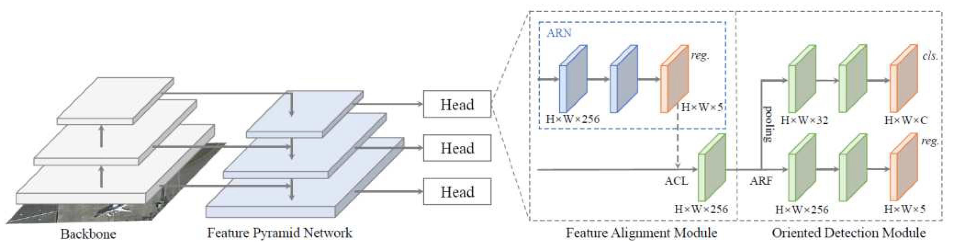
3.1.2. S2A-Net
Figure 8.
The architecture of S2A-Net
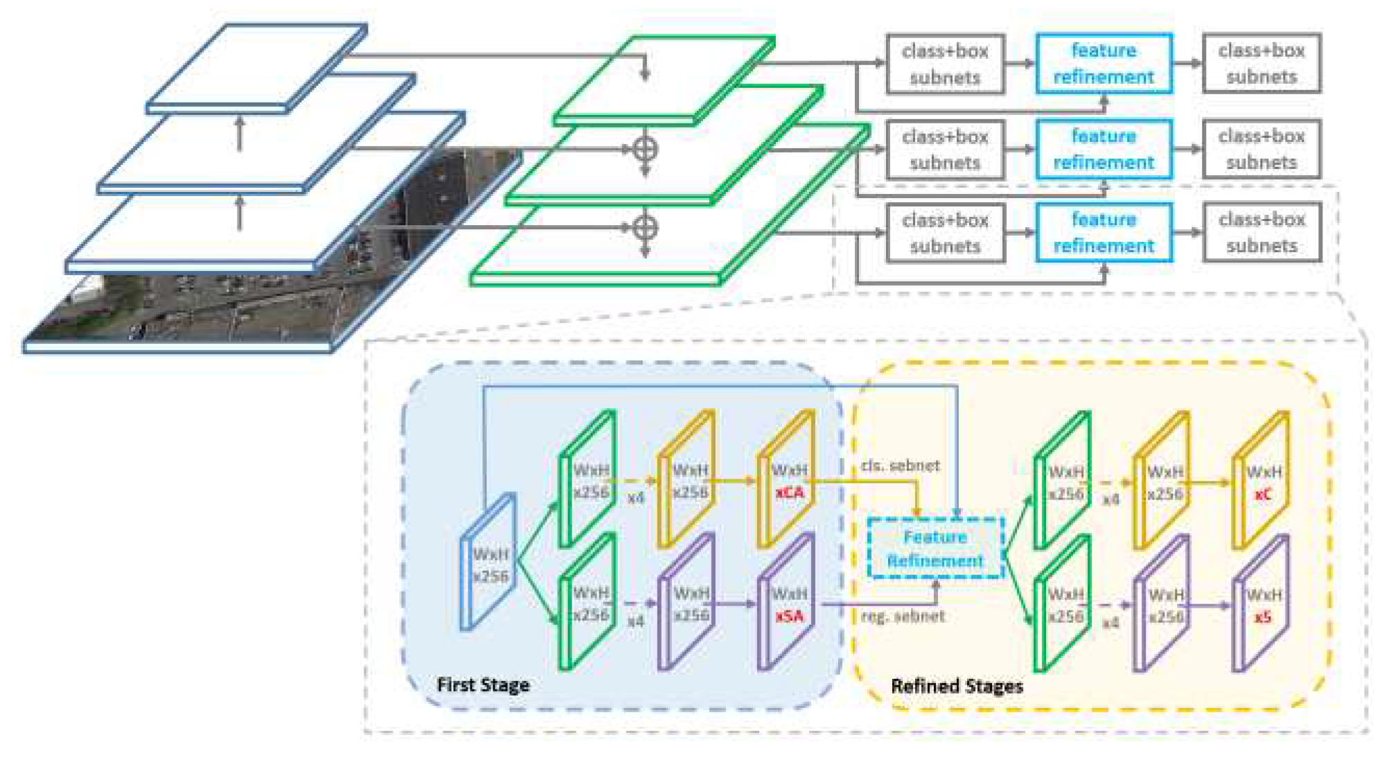
3.1.3. R3Det
Figure 9.
The architecture of R3Det
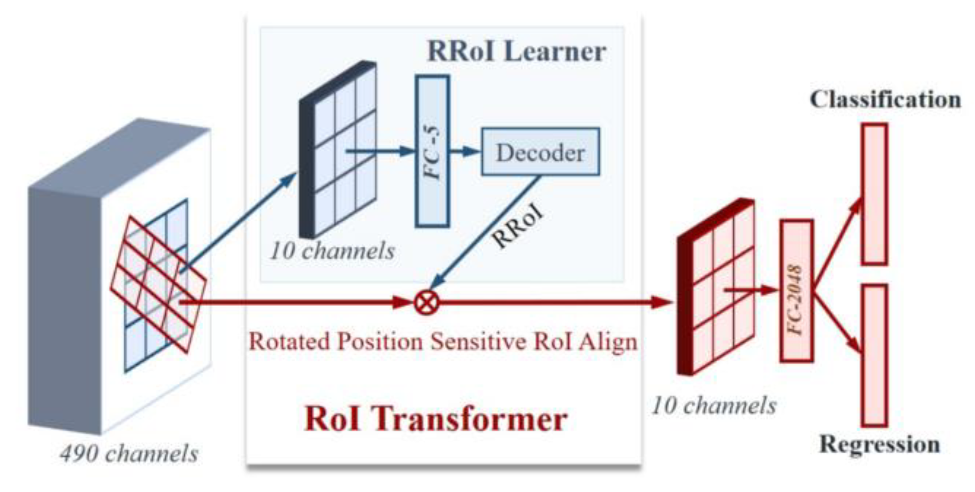
3.1.4. ROI Transformer
Figure 10.
The architecture of ROI Transformert
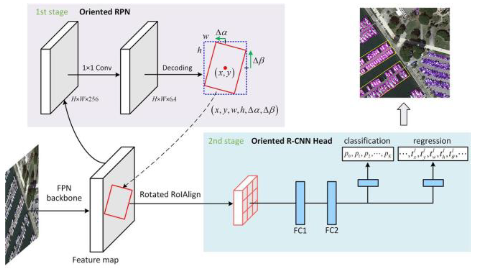
3.1.5. Oriented RCNN
Figure 11.
The architecture of Oriented RCNN
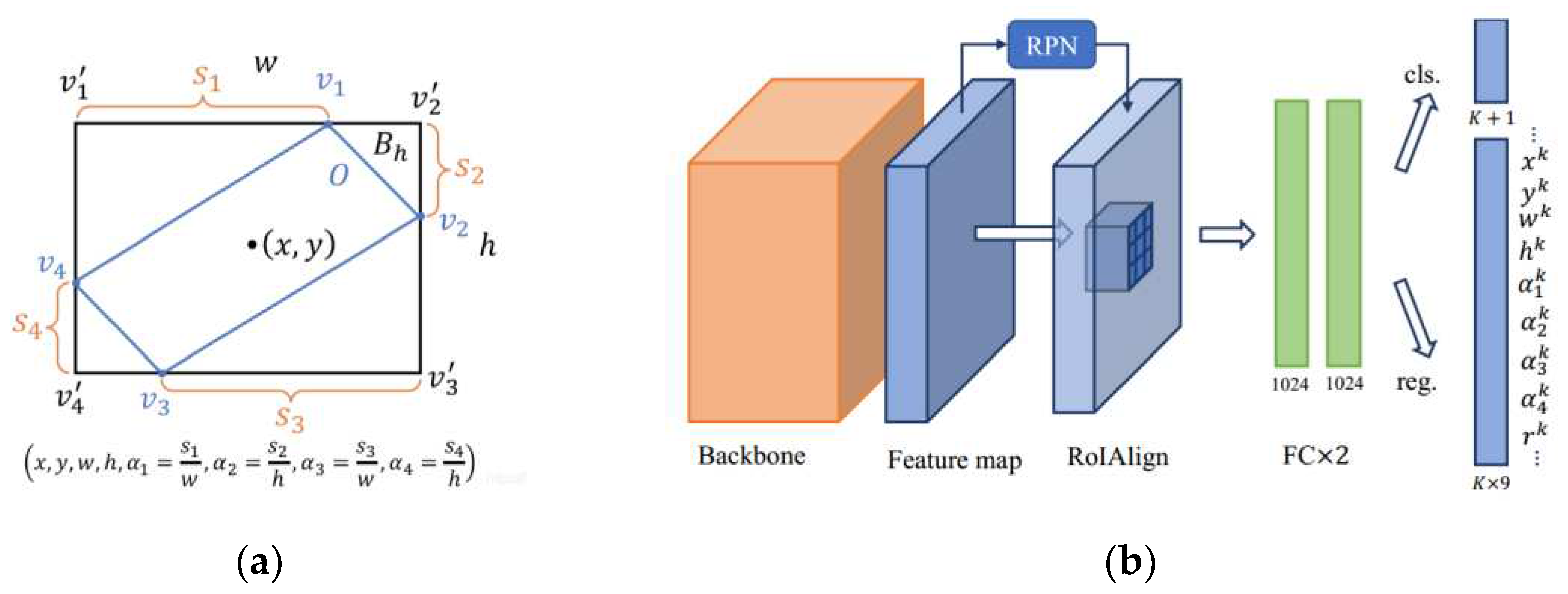
3.1.6. Gliding Vertex
Figure 12.
The architecture of Gliding Vertex
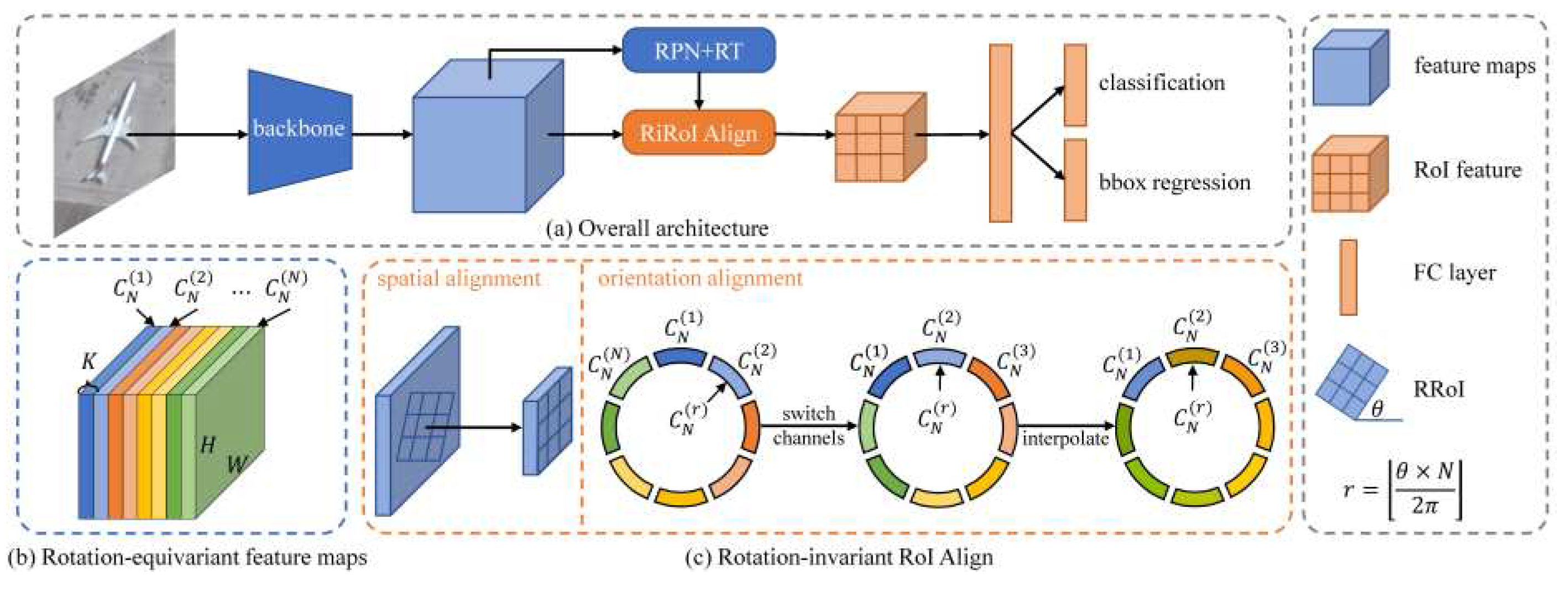
3.1.7. ReDet
Figure 13.
The architecture of ReDet
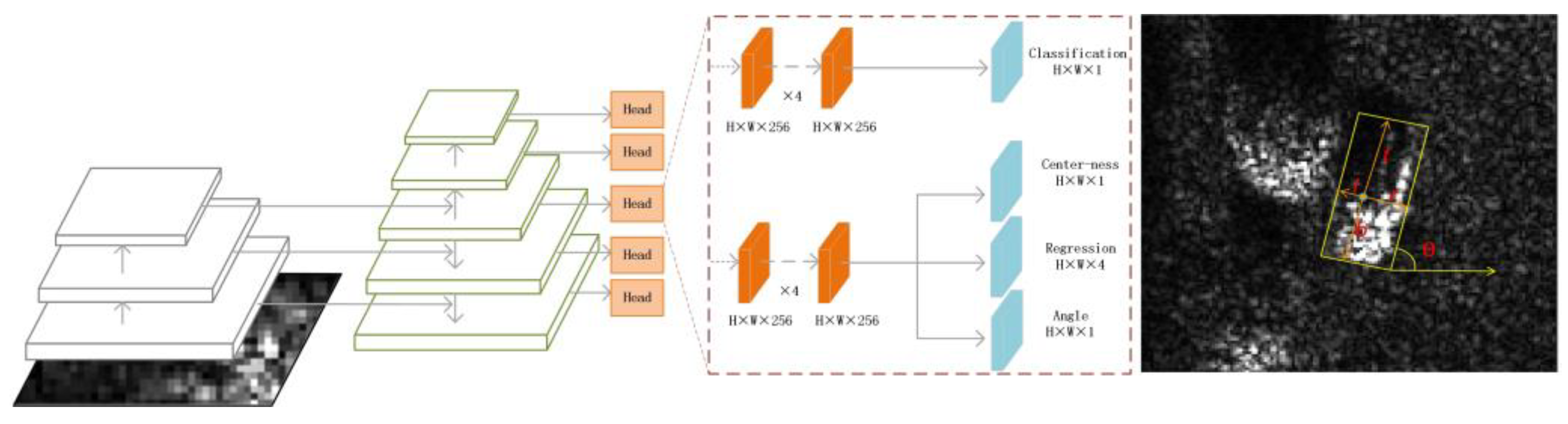
3.1.8. Rotated FCOS
Figure 14.
The architecture of Rotated FCOS
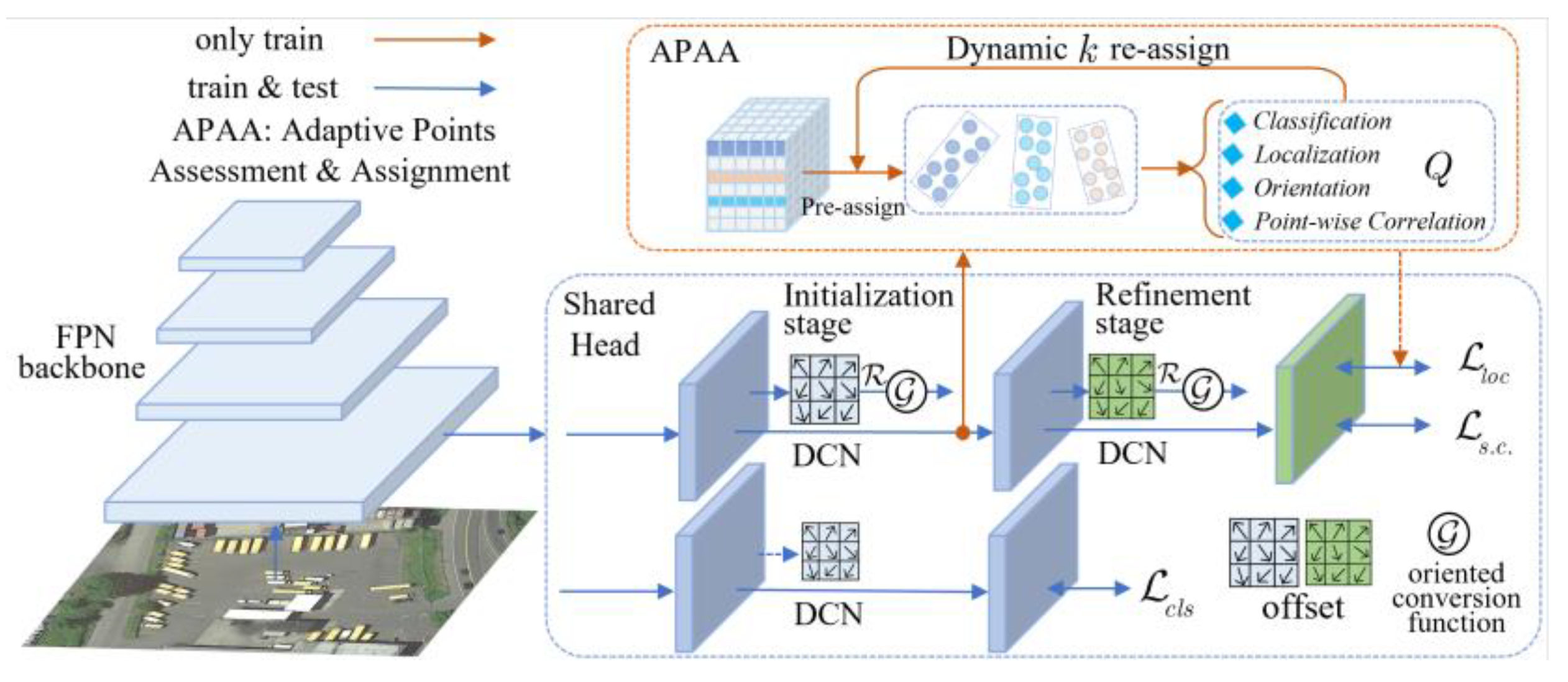
3.1.9. Oriented RepPoints
Figure 15.
The architecture of Oriented RepPoints
3.2. Evaluation Metrics
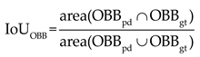
In rotated object detection, the ground truth of the object’s position and the bounding box predicted by the model are oriented bounding boxes. Similar to generic target detection, rotated target detection uses Intersection over Union (IoU) to measure the quality of the predicted bounding box:
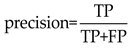
In the classification stage, based on the combination of the prediction bounding box and the ground truth, four results are produced: True Positives (TP), True Negatives (TN), False Negatives (FN), and False Positives (FP). Precision and recall are formulated as follows:
Based on precision and recall, AP is defined as the area under the precision-recall (P-R) curve, while Mean Average Precision (mAP) is defined as the mean of AP values across all classes:
F1 score is the harmonic mean of precision and recall, which is defined as:
3.3. Environment and Details
All experiment were implemented in Ubuntu 20.04.4 with Python3.8.10, Pytorch1.11.0, Cuda11.3. The CPU is Intel i9 11900k @3.5GHz with 32GB RAM, and the GPU is Nvidia GeForce RTX 3090 (24GB) with driver version 470.103.01.
All models involved in this article are implemented through the MMRotate [56] framework. For fair comparison, the backbone network of each detector is ResNet50 [1] pretrained on ImageNet [57] by default, and the neck is FPN [52]. Each image in train set was cropped into 4 pieces of 1024*1024, and the four large-scene images in test set were split into a series of 1024*1024 patches with a stride of 824. To display the performance of each detector on Mix MSTAR as fairly as possible, we simply follow these settings without additional embellishments: data augmentation used random flip with a probability of 0.25 on horizontal, vertical or diagonal axes. Each model was trained for 180 epochs with 2 images per batch. The optimizer was SGD with an initial learning rate of 0.005, momentum of 0.9, and weight decay of 1e-4. L2 norm was adopted for gradient clipping, with the maximum gradient set to 35. The learning rate was decayed by a factor of 10 at the 160th and 220th epochs. Linear preheating was used for the first 500 iterations, with the initial preheating learning rate set to 1/3 of the initial learning rate. Additionally, the IoU threshold in the experiments was set to 0.5 and the confidence threshold was set to 0.3. The mAP and its standard error of all models in this article were obtained by training the network with three different random seeds. The final result is obtained by mapping the prediction of each small picture to the big picture and applying NMS. More details can be found in our log files.
3.4. Result Analysis on Mix MSTAR
The evaluation results for nine models on Mix MSTAR are shown in Table 6 while the class-wise AP results are shown in Table 7. It is important to note that in Table 6, Precision, Recall and F1-score are calculated based on the statistics of all categories of TP, FP and FN.
Combining the results and the previous analysis of the model and the dataset, we can draw the following conclusions:
- In terms of the mAP metric, Oriented RepPoints achieved the best accuracy, which we attribute to its unique proposal approach based on sampling points. This approach successfully combines the deformation convolution and non-axis aligned feature extraction together. Additionally, being a two-stage model, its feature extraction is more accurate. Compared to other refined models, it has more sampling points, up to 9, which makes the extracted features more comprehensive. However, the heavy use of deformation convolution has made its training speed slow. The two-stage model performs better than the single-stage network due to the initial screening of the RPN network. However, the performance of Gliding Vertex is average, which may be due to its failure to use directed proposals in the first stage, resulting in inaccurate feature extraction. ReDet has poor performance, possibly because the rotation-invariant network used in ReDet is not suitable for SAR images with a low depression. Mix MSTAR are simulated at a depression of 15°, and the shadow area is quite large, leading to significant imaging differences for the same object under different azimuth angles. For example, rotating a vehicle image at an angle of θ by α degrees would produce an image that is significantly different from the image of the same vehicle captured at (θ+α) degrees, which may cause ReResNet to extract incorrect rotation-invariant features. Compared to single-stage models, refined-stage models demonstrate a significant performance improvement, suggesting that refined-stage models are more accurate in extracting non-axis aligned features of rotated objects, which can reduce the gap between refined-stage models and two-stage models. While the performance of R3Det is slightly inferior, it is similar to ReDet, and its reason may lie in the sampling points in its refined stage, which are fixed at the four corners and the center point. In low-pitch-angle SAR images, one vertex far from the radar sensor is necessarily shaded, which means that the feature extraction of the sampling point interferes with the overall feature expression. S2A-Net uses deformation convolution, with the position of the sampling point being learnable. Although there is still a probability of collecting data from the shaded vertexes, there are nine sampling points, which dilutes the influence of features from the shaded vertexes.
- In terms of speed, Rotated FCOS performs the best, benefiting from its anchor-free design and full convolution structure. Its parameters and computation are both lower than those of Rotated Retinanet. In contrast, other models use deformation convolution or non-conventional feature alignment convolution or non-full convolution structures, making network speed relatively slow. Due to its special rotation-equivariant convolution, ReDet has the slowest inference speed, even though its parameter and computation is the lowest. In terms of parameter quantities, the two anchor-free models and the single-stage model have fewer parameters than other models. The RPN of ROI Transformer requires two stages to extract the rotation ROI, so it has the most parameters. In terms of computation, due to its multi-head design, the detection head of the single-stage model is too cumbersome, making its computation not significantly lower than that of the two-stage model. However, Mix MSTAR is a small target data set, with most of its ground truth width being below 32. After five times downsampling, its localization information has been lost. Better balance may be obtained by optimizing the regression subnetwork of layers with downsample sizes greater than 32.
- In terms of precision and recall metrics, all networks tend to maintain high recall. As using inter-class NMS limits the Recall integration range of mAP, like the DOTA, inter-class NMS is disabled. But this resulted in lower accuracy. Among them, ROI Transformer achieved a balance between accuracy and recall and obtained the highest F1 score.
- From the results presented in Table 7, it is evident that the fine-grained classification result of T72 tank is poor and has a significant impact on all detectors. Figure 16a further illustrates this point, as the confusion matrix of Oriented RepPoints indicates a considerable number of FP assigned to wrong subtypes of the T72 tank, which is also observed in cross-category confusion intervals such as BTR70-BTR60, 2S1-T62, and T72-T62. Another notable observation is the poor detection effect of BMP2 under EOC, as indicated in the confusion matrix. Many BMP2 subtypes that didn’t appear in the train set are mistaken for other vehicles in testing. Figure 16b depicts the P-R curves of all detectors.
- Figure 17 presents the detection results of three detectors on the same picture. The results showed that the localization of the vehicles was accurate, but the recognition accuracy was not high, with a small number of false positives and misses. Additionally, we discovered two unknown vehicles in the scene, which were initially hidden among the clutters and did not belong to the Chips. One vehicle was recognized as T62 by all three models, while the other vehicle was classified as background, possibly because its area was significantly larger than the vehicles in the Mix MSTAR. This indicates that the model trained by Mix MSTAR has the ability to recognize real vehicles.
4. Discussion
For a synthetic dataset that aims to become a detection benchmark, both fidelity and effectiveness are essential. However, in the production of Mix MSTAR, it is necessary to manually extract vehicles from Chips and fuse radar data collected under different modes before generating the final image. Thus, there are two potential problems in this process, which will affect the visual effectiveness of the synthetic images:
- Artificial traces: The vehicle masks manually extracted can alter the contour features of the vehicles and leave artificial traces in the synthetic images. Even though Gaussian smoothing was applied to reduce this effect on the vehicle edges, theoretically, these traces could still be utilized by overfitting models to identify targets.
- Data variance: The vehicle and background data in Mix MSTAR were collected under different operating modes. Although we harmonized the data amplitude based on reasonable assumptions, Chips was collected using spotlight mode, while Clutters used strip mode. The two different scanning modes of radar can cause variances in the image style (particularly spatial distribution) of foreground and background in the synthetic images. This could lead detection models to find some cheating shortcuts due to the non-realistic effects of the synthetic images, failing to extract common image features.
To address these concerns, we designed two separate experiments to demonstrate the reliability of the synthetic dataset.
4.1. The Artificial Traces Problem
To address the potential problem of artificial traces and to prove the fidelity of the synthetic dataset, our approach was to use a model trained on Mix MSTAR to detect intact vehicle images. We randomly selected 25 images from the Chips and expanded them to 204x204 to maintain their original size. These images were then stitched into a 1024x1024 large image, which was input into the ROI Transformer trained on Mix MSTAR. As shown in Figure 18a, all these intact vehicles were accurately localized, with a classification accuracy of 80%.
However, an accuracy of 80% is not an ideal result, as the background in Chips is quite simple and the five misidentified vehicles were all subtypes of T72. As a comparison experiment, we trained and tested ResNet18 as a classification model on the 20 classes Chips of MSTAR, following the same partition strategy as Mix MSTAR, and the classifier easily achieved 92.22% accuracy. However, we found through class activation maps [58] that since each type of vehicle in MSTAR was captured at different angles, but at the same location, the high correlation between the backgrounds in Chips causes the classifier to focus more on the terrain than the vehicles themselves. As shown in Figure 19, the two subtypes of T72 were identified based on their tracks and unusual vegetation, with recognition rates of 98.77% and 100%. However, the accuracy of the two T72 subtypes that did not benefit from background correlation was only 73.17% and 66.67%, respectively. This phenomenon also existed in other types of vehicles, indicating that the training results of using background-correlated Chips are actually unreliable.
Through the detection of intact vehicles in real images, we have proven that the artificial traces generated in the process of mask extraction did not affect the models. On the contrary, benefit from the mask extraction and background transfer, Mix MSTAR eliminated background correlation, allowing models trained on the high-fidelity synthetic images to focus on vehicle features, such as shadows and bright spots, as shown in Figure 18b.
4.2. The Data Variance Problem
To address potential data variance problem and demonstrate the authentic detection capability of models obtained from Mix MSTAR, we designed the following experiment to prove the effectiveness of the Mix MSTAR. The real dataset, Mini SAR was used to train and evaluate models pretrained on Mix MSTAR and those not pretrained on Mix MSTAR. For the pretrained models, we froze the weights of first stage of the backbone, forcing the network to extract features in the same way as it does with synthetic images. The non-pretrained models were loaded from ImageNet weights as a regular setting. We selected nine images containing vehicles as the dataset, and seven were used for training and two for validation. The images were divided into 1024x1024 images with a stride of 824. Since the dataset was very small, the training process of each network was unstable. Therefore, we extended the number of iterations to 240 epochs, recorded the mAP of the model on the validation set after each epoch, and set the learning rate reducing 10 folds at epoch 160 and epoch 220, with all other settings consistent with those in the Mix MSTAR experiments. It is worth noting that there is no perfect unified training setting that can fit all detectors due to their different feature extraction capabilities and the propensity for overfitting on the small dataset. Thus, we record the best results of the validation set during training in Table 8.
Firstly, as shown in Table 8, all models obtained an improvement after being pretrained on Mix MSTAR. Since the weights of the first layer are frozen after pretraining, this indicates that the models effectively learn how to extract general underlying features from SAR images. Secondly, since the validation set contains only two images, the results of non-pretrained models were very unstable, but the standard errors of all models were significantly reduced after pretraining on Mix MSTAR. Additionally, as shown in Figure 20, the pretrained models had very rapid loss reduction during the training process. See Figure 21, after a few epochs, their accuracy on the validation set increased significantly, and ultimately reached a relatively stable result. However, the loss and mAP of the non-pretrained models were unstable.
We noticed that Rotated RetinaNet and Rotated FCOS are very sensitive to the random seed initialization, making them prone to training failure. This may be due to the weak ability of single-stage detectors in feature extraction, which makes it difficult for them to learn effective feature extraction capabilities from a small quantity of data. Therefore, we conducted a comparison experiment in which we added the Mix MSTAR train set to the Mini SAR train set to increase the data size when training the non-pretrained models. As shown in Table 9, both single-stage models obtained significant improvements after mixed training with the two datasets. As seen in Figure 22, pretraining on Mix MSTAR or mixed training with Mix MSTAR both resulted in increased recall and precision of the models, achieving more accurate bounding box regression.
Based on the above comparison experiments using real data, we have demonstrated the effectiveness of Mix MSTAR, indicating that synthetic data can also help networks learn how to extract features from real SAR images, thereby proving the effectiveness and transferability ability of the Mix MSTAR. In addition, the experiment shows that the unstable Mini SAR is not suitable as the benchmark dataset for algorithm comparison, especially for the single-stage model, and also verifies that the Mix MSTAR is effective in addressing the problem of insufficient real data for SAR vehicle detection.
4.3. Potential Application
As more and more creative work leverages synthetic data to advance human understanding towards the real world, Mix MSTAR, as the first public SAR vehicle multi-class detection dataset, has many potential applications. Here, we envision two potential use cases:
- SAR image generation. While mutual conversion between optical and SAR imagery is no longer a groundbreaking achievement, current style transfer methods between visible light and SAR are primarily used for low-resolution terrain classification [59]. Given the scarcity of high-resolution SAR images and the abundance of high-resolution labeled visible light images, a promising avenue is to combine the two to generate more synthetic SAR images to address the lack of labeled SAR data and ultimately improve real SAR object detection. Although the synthetic image obtained in this way can not be used for model evaluation, it can help the detection model to obtain stronger positioning ability when detecting real SAR objects through pre-training or mixed training. Figure 23 demonstrates an example of using CycleGAN [60] to transfer vehicle images from DOTA domain to the Mix MSTAR domain.
- Out-of-distribution detection. Out-of-distribution detection, or OOD detection, aims to detect test samples that drawn from a distribution that is different from the training distribution [61]. Using the model trained by synthetic images to classify real images was regarded as a challenging problem in SAMPLE[25]. Unlike visible light imagery, SAR imaging is heavily influenced by sensor operating parameters, resulting in significant stylistic differences between images captured under different condition. Our experiments found that current models’ performance on different SAR datasets is poorly generalizable. If reannotation and retraining are required for every new dataset, the cost will increase significantly, exacerbating the scarcity of SAR imagery and limiting the application scenarios of SAR-ATR. Therefore, it is an important research direction to use the limited labeled datasets to detect more unlabeled data. We used the Redet model trained on Mix MSTAR to detect real vehicles in a image from FARAD KA BAND. Due to resolution differences, three vehicles were detected dafter applying multi-scale test techniques as shown in Figure 24.
5. Conclusions
This research released a large-scale SAR image synthesis dataset for multi-class rotated vehicle detection and proposed a paradigm for realistically fusing SAR data from different domains. Upon evaluating nine different benchmark detectors, we found that fine-grained classification makes Mix MSTAR highly challenging, with considerable room for improving object detection performance. Additionally, to address concerns over potential artificial traces and data variance in synthetic data, we conducted two experiments to demonstrate the fidelity and effectiveness of Mix MSTAR. Finally, we summarized two potential applications of Mix MSTAR and call on the community to enhanced communication and cooperation in the SAR data sharing to alleviate the scarcity of data and promote the development of SAR.
Author Contributions
Conceptualization, Z.L. and S.L.; methodology, Z.L.; software, S.L.; validation, Z.L., S.L. and Y.W.; formal analysis, Z.L.; investigation, Z.L.; resources, Z.L.; data curation, S.L.; writing—original draft preparation, S.L.; writing—review and editing, Z.L.; visualization, Z.L.; supervision, Z.L.; project administration, Z.L.; funding acquisition, Y.W. All authors have read and agreed to the published version of the manuscript.
Funding
This research was funded in part by the National Natural Science Foundation of China under Grant 61905285 and in part by the Young Talent Fund of University Association for Science and Technology in Shaanxi, China, under Grant 20200704.
Data Availability Statement
The dataset and the training log files can be obtained by contacting us through lonsonjay@163.com mailbox, which is very welcome.
Conflicts of Interest
The authors declare no conflict of interest.
References
- He, K.; Zhang, X.; Ren, S.; Sun, J. Deep residual learning for image recognition. In Proceedings of the Proceedings of the IEEE conference on computer vision and pattern recognition, 2016; pp. 770–778. [Google Scholar]
- Ren, S.; He, K.; Girshick, R.; Sun, J. Faster r-cnn: Towards real-time object detection with region proposal networks. Advances in neural information processing systems 2015, 28. [Google Scholar] [CrossRef] [PubMed]
- Xia, G.-S.; Bai, X.; Ding, J.; Zhu, Z.; Belongie, S.; Luo, J.; Datcu, M.; Pelillo, M.; Zhang, L. DOTA: A large-scale dataset for object detection in aerial images. In Proceedings of the Proceedings of the IEEE conference on computer vision and pattern recognition, 2018; pp. 3974–3983. [Google Scholar]
- Li, J.; Qu, C.; Shao, J. Ship detection in SAR images based on an improved faster R-CNN. In Proceedings of the 2017 SAR in Big Data Era: Models, Methods and Applications (BIGSARDATA), 2017; pp. 1–6. [Google Scholar]
- Wang, Y.; Wang, C.; Zhang, H.; Dong, Y.; Wei, S. A SAR dataset of ship detection for deep learning under complex backgrounds. remote sensing 2019, 11, 765. [Google Scholar] [CrossRef]
- Xian, S.; Zhirui, W.; Yuanrui, S.; Wenhui, D.; Yue, Z.; Kun, F. AIR-SARShip-1.0: High-resolution SAR ship detection dataset. J. Radars 2019, 8, 852–863. [Google Scholar] [CrossRef]
- Wei, S.; Zeng, X.; Qu, Q.; Wang, M.; Su, H.; Shi, J. HRSID: A high-resolution SAR images dataset for ship detection and instance segmentation. Ieee Access 2020, 8, 120234–120254. [Google Scholar] [CrossRef]
- Zhang, T.; Zhang, X.; Ke, X.; Zhan, X.; Shi, J.; Wei, S.; Pan, D.; Li, J.; Su, H.; Zhou, Y. LS-SSDD-v1. 0: A deep learning dataset dedicated to small ship detection from large-scale Sentinel-1 SAR images. Remote Sensing 2020, 12, 2997. [Google Scholar] [CrossRef]
- Lei, S.; Lu, D.; Qiu, X.; Ding, C. SRSDD-v1. 0: A high-resolution SAR rotation ship detection dataset. Remote Sensing 2021, 13, 5104. [Google Scholar] [CrossRef]
- The Air Force Moving and Stationary Target Recognition Database. Available online: https://www.sdms.afrl.af.mil/datasets/mstar/ (accessed on 10 March 2011).
- Zhang, L.; Leng, X.; Feng, S.; Ma, X.; Ji, K.; Kuang, G.; Liu, L. Domain knowledge powered two-stream deep network for few-shot SAR vehicle recognition. IEEE Transactions on Geoscience and Remote Sensing 2021, 60, 1–15. [Google Scholar] [CrossRef]
- Zhang, L.; Leng, X.; Feng, S.; Ma, X.; Ji, K.; Kuang, G.; Liu, L. Azimuth-Aware Discriminative Representation Learning for Semi-Supervised Few-Shot SAR Vehicle Recognition. Remote Sensing 2023, 15, 331. [Google Scholar] [CrossRef]
- SANDIA FARAD SAR DATA COLLECTION – X BAND – 4″ RESOLUTION. Available online: https://www.sandia.gov/files/radar/complex-data/FARAD_X_BAND.zip (accessed on 30 April 2023).
- SANDIA FARAD SAR DATA COLLECTION – KA BAND – 4″ RESOLUTION. Available online: https://www.sandia.gov/files/radar/complex-data/FARAD_KA_BAND.zip (accessed on 30 April 2023).
- SANDIA Spotlight SAR. Available online: https://www.sandia.gov/files/radar/complex-data/20060214.zip (accessed on 30 April 2023).
- SANDIA Mini SAR Complex Imagery. Available online: https://www.sandia.gov/files/radar/complex-data/MiniSAR20050519p0009image003.zip (accessed on 30 April 2023).
- Casteel Jr, C.H.; Gorham, L.A.; Minardi, M.J.; Scarborough, S.M.; Naidu, K.D.; Majumder, U.K. A challenge problem for 2D/3D imaging of targets from a volumetric data set in an urban environment. In Proceedings of the Algorithms for Synthetic Aperture Radar Imagery XIV, 2007; pp. 97–103. [Google Scholar]
- Goodfellow, I.; Pouget-Abadie, J.; Mirza, M.; Xu, B.; Warde-Farley, D.; Ozair, S.; Courville, A.; Bengio, Y. Generative adversarial networks. Communications of the ACM 2020, 63, 139–144. [Google Scholar] [CrossRef]
- Gao, F.; Yang, Y.; Wang, J.; Sun, J.; Yang, E.; Zhou, H. A deep convolutional generative adversarial networks (DCGANs)-based semi-supervised method for object recognition in synthetic aperture radar (SAR) images. Remote Sensing 2018, 10, 846. [Google Scholar] [CrossRef]
- Cui, Z.; Zhang, M.; Cao, Z.; Cao, C. Image data augmentation for SAR sensor via generative adversarial nets. IEEE Access 2019, 7, 42255–42268. [Google Scholar] [CrossRef]
- Vignaud, L. GAN4SAR: Generative Adversarial Networks for Synthetic Aperture Radar imaging of targets signature. In Proceedings of the SET-273 Specialists Meeting on Multidimensional Radar Imaging and ATR-CfP, 2021. [Google Scholar]
- Auer, S.; Bamler, R.; Reinartz, P. RaySAR-3D SAR simulator: Now open source. In Proceedings of the 2016 IEEE International Geoscience and Remote Sensing Symposium (IGARSS), 2016; pp. 6730–6733. [Google Scholar]
- Malmgren-Hansen, D.; Kusk, A.; Dall, J.; Nielsen, A.A.; Engholm, R.; Skriver, H. Improving SAR automatic target recognition models with transfer learning from simulated data. IEEE Geoscience and remote sensing Letters 2017, 14, 1484–1488. [Google Scholar] [CrossRef]
- Cha, M.; Majumdar, A.; Kung, H.; Barber, J. Improving SAR automatic target recognition using simulated images under deep residual refinements. In Proceedings of the 2018 IEEE International Conference on Acoustics, Speech and Signal Processing (ICASSP), 2018; pp. 2606–2610. [Google Scholar]
- Lewis, B.; Scarnati, T.; Sudkamp, E.; Nehrbass, J.; Rosencrantz, S.; Zelnio, E. A SAR dataset for ATR development: the Synthetic and Measured Paired Labeled Experiment (SAMPLE). In Proceedings of the Algorithms for Synthetic Aperture Radar Imagery XXVI, 2019; pp. 39–54. [Google Scholar]
- Chen, S.; Wang, H.; Xu, F.; Jin, Y.-Q. Target classification using the deep convolutional networks for SAR images. IEEE transactions on geoscience and remote sensing 2016, 54, 4806–4817. [Google Scholar] [CrossRef]
- Han, Z.-s.; Wang, C.-p.; Fu, Q. Arbitrary-oriented target detection in large scene sar images. Defence Technology 2020, 16, 933–946. [Google Scholar] [CrossRef]
- Sun, Y.; Wang, W.; Zhang, Q.; Ni, H.; Zhang, X. Improved YOLOv5 with transformer for large scene military vehicle detection on SAR image. In Proceedings of the 2022 7th International Conference on Image, Vision and Computing (ICIVC), 2022; pp. 87–93. [Google Scholar]
- labelme: Image Polygonal Annotation with Python (polygon, rectangle, circle, line, point and image-level flag annotation). Available online: https://github.com/wkentaro/labelme.
- Cong, W.; Zhang, J.; Niu, L.; Liu, L.; Ling, Z.; Li, W.; Zhang, L. Dovenet: Deep image harmonization via domain verification. In Proceedings of the Proceedings of the IEEE/CVF conference on computer vision and pattern recognition, 2020; pp. 8394–8403. [Google Scholar]
- Reinhard, E.; Adhikhmin, M.; Gooch, B.; Shirley, P. Color transfer between images. IEEE Computer graphics and applications 2001, 21, 34–41. [Google Scholar] [CrossRef]
- Pérez, P.; Gangnet, M.; Blake, A. Poisson image editing. In ACM SIGGRAPH 2003 Papers; 2003; pp. 313–318. [Google Scholar]
- Sunkavalli, K.; Johnson, M.K.; Matusik, W.; Pfister, H. Multi-scale image harmonization. ACM Transactions on Graphics (TOG) 2010, 29, 1–10. [Google Scholar] [CrossRef]
- Tsai, Y.-H.; Shen, X.; Lin, Z.; Sunkavalli, K.; Lu, X.; Yang, M.-H. Deep image harmonization. In Proceedings of the Proceedings of the IEEE Conference on Computer Vision and Pattern Recognition, 2017; pp. 3789–3797.
- Zhang, L.; Wen, T.; Shi, J. Deep image blending. In Proceedings of the Proceedings of the IEEE/CVF Winter Conference on Applications of Computer Vision, 2020; pp. 231–240.
- Ling, J.; Xue, H.; Song, L.; Xie, R.; Gu, X. Region-aware adaptive instance normalization for image harmonization. In Proceedings of the Proceedings of the IEEE/CVF conference on computer vision and pattern recognition, 2021; pp. 9361–9370.
- Schumacher, R.; Rosenbach, K. ATR of battlefield targets by SAR classification results using the public MSTAR dataset compared with a dataset by QinetiQ UK. In Proceedings of the RTO SET Symposium on Target Identification and Recognition Using RF Systems, 2004. [Google Scholar]
- Schumacher, R.; Schiller, J. Non-cooperative target identification of battlefield targets-classification results based on SAR images. In Proceedings of the IEEE International Radar Conference; 2005; pp. 167–172. [Google Scholar]
- Geng, Z.; Xu, Y.; Wang, B.-N.; Yu, X.; Zhu, D.-Y.; Zhang, G. Target Recognition in SAR Images by Deep Learning with Training Data Augmentation. Sensors 2023, 23, 941. [Google Scholar] [CrossRef]
- Lin, T.-Y.; Maire, M.; Belongie, S.; Hays, J.; Perona, P.; Ramanan, D.; Dollár, P.; Zitnick, C.L. Microsoft coco: Common objects in context. In Proceedings of the Computer Vision–ECCV 2014: 13th European Conference, Zurich, Switzerland, September 6-12, 2014, Proceedings, Part V 13, 2014; pp. 740–755. [Google Scholar]
- Lin, T.-Y.; Goyal, P.; Girshick, R.; He, K.; Dollár, P. Focal loss for dense object detection. In Proceedings of the Proceedings of the IEEE international conference on computer vision, 2017; pp. 2980–2988.
- Han, J.; Ding, J.; Li, J.; Xia, G.-S. Align deep features for oriented object detection. IEEE Transactions on Geoscience and Remote Sensing 2021, 60, 1–11. [Google Scholar] [CrossRef]
- Dai, J.; Qi, H.; Xiong, Y.; Li, Y.; Zhang, G.; Hu, H.; Wei, Y. Deformable convolutional networks. In Proceedings of the Proceedings of the IEEE international conference on computer vision, 2017; pp. 764–773.
- Yang, X.; Yan, J.; Feng, Z.; He, T. R3det: Refined single-stage detector with feature refinement for rotating object. In Proceedings of the Proceedings of the AAAI conference on artificial intelligence, 2021; pp. 3163–3171.
- Ding, J.; Xue, N.; Long, Y.; Xia, G.-S.; Lu, Q. Learning roi transformer for oriented object detection in aerial images. In Proceedings of the Proceedings of the IEEE/CVF Conference on Computer Vision and Pattern Recognition, 2019; pp. 2849–2858.
- Xie, X.; Cheng, G.; Wang, J.; Yao, X.; Han, J. Oriented R-CNN for object detection. In Proceedings of the Proceedings of the IEEE/CVF International Conference on Computer Vision, 2021; pp. 3520–3529.
- Ma, J.; Shao, W.; Ye, H.; Wang, L.; Wang, H.; Zheng, Y.; Xue, X. Arbitrary-oriented scene text detection via rotation proposals. IEEE transactions on multimedia 2018, 20, 3111–3122. [Google Scholar] [CrossRef]
- Xu, Y.; Fu, M.; Wang, Q.; Wang, Y.; Chen, K.; Xia, G.-S.; Bai, X. Gliding vertex on the horizontal bounding box for multi-oriented object detection. IEEE transactions on pattern analysis and machine intelligence 2020, 43, 1452–1459. [Google Scholar] [CrossRef]
- Han, J.; Ding, J.; Xue, N.; Xia, G.-S. Redet: A rotation-equivariant detector for aerial object detection. In Proceedings of the Proceedings of the IEEE/CVF Conference on Computer Vision and Pattern Recognition, 2021; pp. 2786–2795.
- Weiler, M.; Cesa, G. General e (2)-equivariant steerable cnns. Advances in Neural Information Processing Systems 2019, 32. [Google Scholar]
- Tian, Z.; Shen, C.; Chen, H.; He, T. Fcos: Fully convolutional one-stage object detection. In Proceedings of the Proceedings of the IEEE/CVF international conference on computer vision, 2019; pp. 9627–9636.
- Lin, T.-Y.; Dollár, P.; Girshick, R.; He, K.; Hariharan, B.; Belongie, S. Feature pyramid networks for object detection. In Proceedings of the Proceedings of the IEEE conference on computer vision and pattern recognition, 2017; pp. 2117–2125.
- Yang, Z.; Liu, S.; Hu, H.; Wang, L.; Lin, S. Reppoints: Point set representation for object detection. In Proceedings of the Proceedings of the IEEE/CVF international conference on computer vision, 2019; pp. 9657–9666.
- Li, W.; Chen, Y.; Hu, K.; Zhu, J. Oriented reppoints for aerial object detection. In Proceedings of the Proceedings of the IEEE/CVF Conference on Computer Vision and Pattern Recognition, 2022; pp. 1829–1838.
- Rezatofighi, H.; Tsoi, N.; Gwak, J.; Sadeghian, A.; Reid, I.; Savarese, S. Generalized intersection over union: A metric and a loss for bounding box regression. In Proceedings of the Proceedings of the IEEE/CVF conference on computer vision and pattern recognition, 2019; pp. 658–666.
- Zhou, Y.; Yang, X.; Zhang, G.; Wang, J.; Liu, Y.; Hou, L.; Jiang, X.; Liu, X.; Yan, J.; Lyu, C. MMRotate: A Rotated Object Detection Benchmark using PyTorch. In Proceedings of the Proceedings of the 30th ACM International Conference on Multimedia, 2022; pp. 7331–7334.
- Deng, J.; Dong, W.; Socher, R.; Li, L.-J.; Li, K.; Fei-Fei, L. Imagenet: A large-scale hierarchical image database. In Proceedings of the 2009 IEEE conference on computer vision and pattern recognition, 2009; pp. 248–255.
- Selvaraju, R.R.; Cogswell, M.; Das, A.; Vedantam, R.; Parikh, D.; Batra, D. Grad-cam: Visual explanations from deep networks via gradient-based localization. In Proceedings of the Proceedings of the IEEE international conference on computer vision, 2017; pp. 618–626.
- Yang, X.; Zhao, J.; Wei, Z.; Wang, N.; Gao, X. SAR-to-optical image translation based on improved CGAN. Pattern Recognition 2022, 121, 108208. [Google Scholar] [CrossRef]
- Zhu, J.-Y.; Park, T.; Isola, P.; Efros, A.A. Unpaired image-to-image translation using cycle-consistent adversarial networks. In Proceedings of the Proceedings of the IEEE international conference on computer vision, 2017; pp. 2223–2232.
- Yang, J.; Zhou, K.; Li, Y.; Liu, Z. Generalized out-of-distribution detection: A survey. arXiv arXiv:2110.11334 2021.
Figure 1.
Three data generation methods around MSTAR. (a) Some sample pictures from [20] based on GANs; (b) Some sample pictures from [25] based on CAD 3D modeling and electromagnetic calculation simulation; (c) A sample picture from [26] based on background transferring.
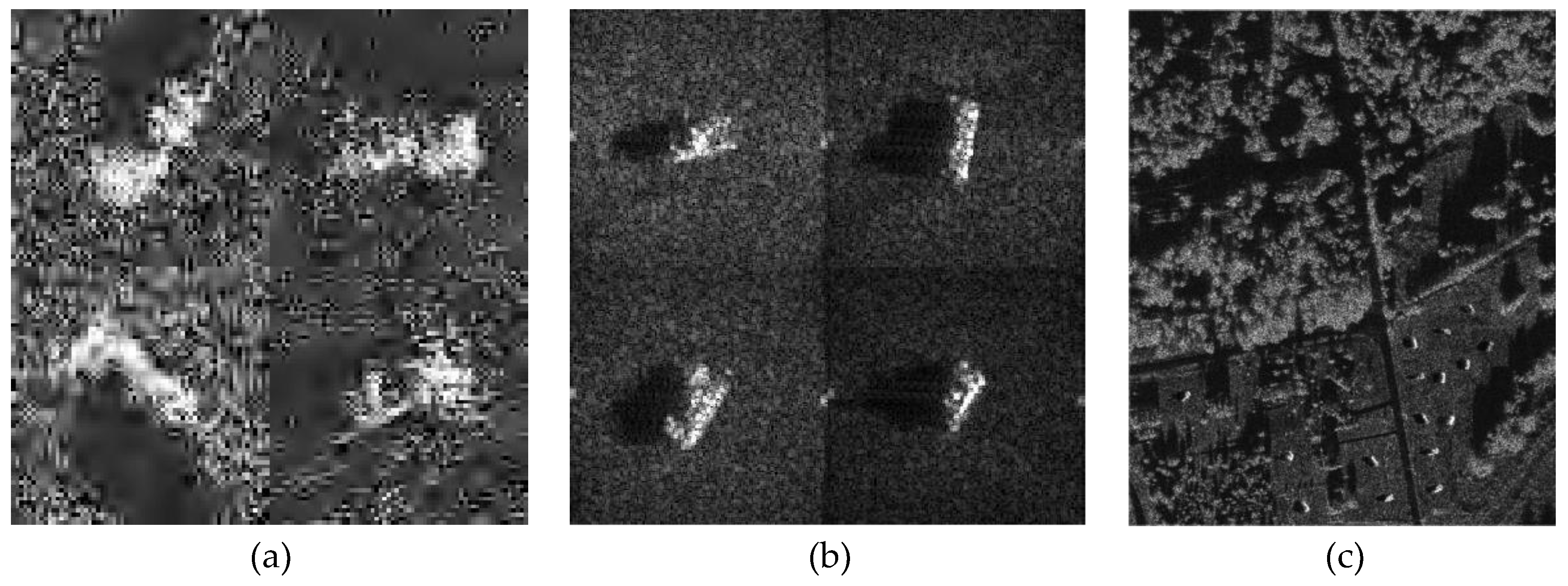
Figure 2.
The pipeline of construct the synthetic dataset.
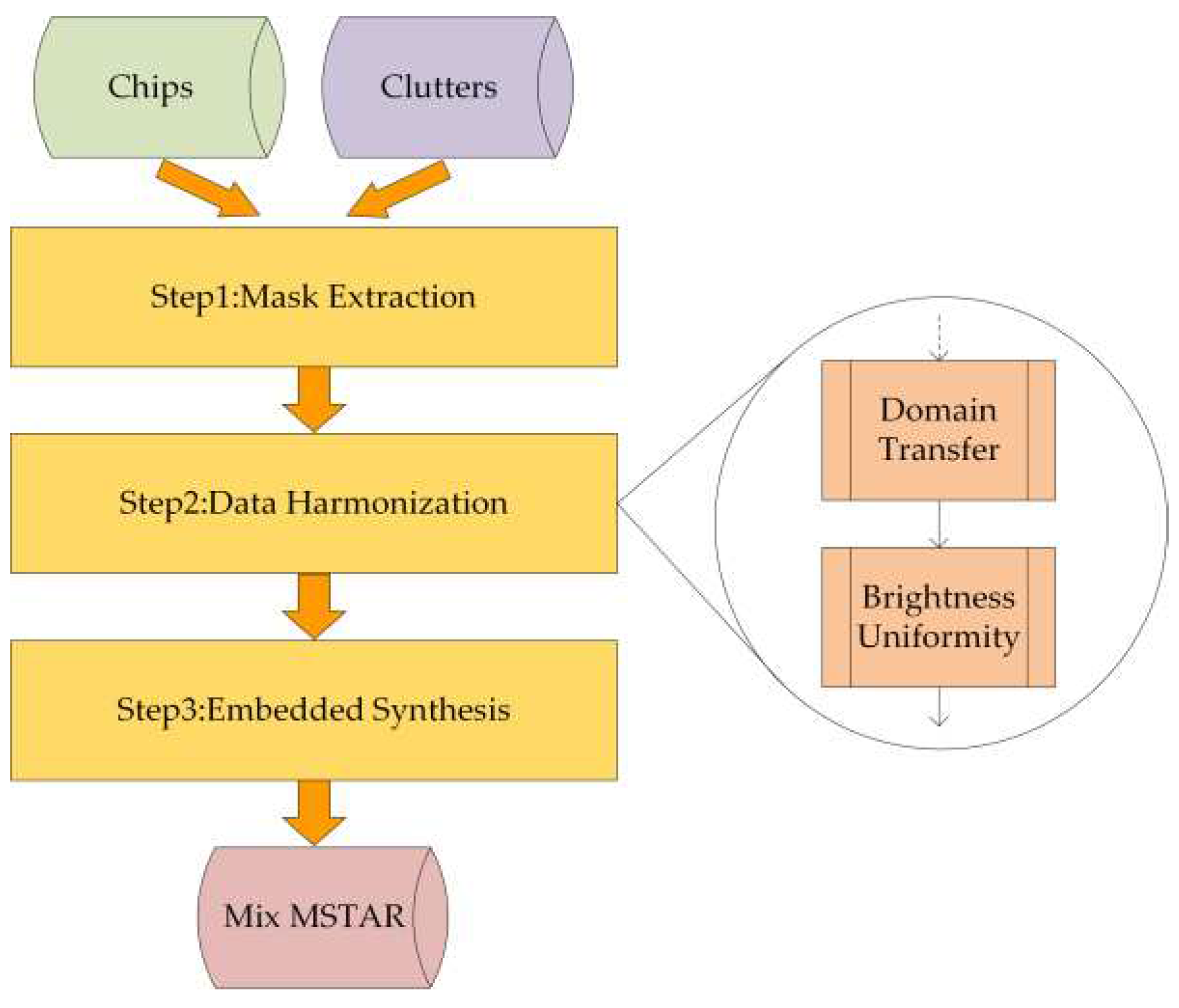
Figure 3.
Vehicle segmentation label, containing a mask of the vehicle and its shadow and a rotated bounding box of its visually salient part. (a) The label of the vehicle when the boundary is relatively clear; (b) The label of the vehicle when the boundary is blurred.
Figure 3.
Vehicle segmentation label, containing a mask of the vehicle and its shadow and a rotated bounding box of its visually salient part. (a) The label of the vehicle when the boundary is relatively clear; (b) The label of the vehicle when the boundary is blurred.
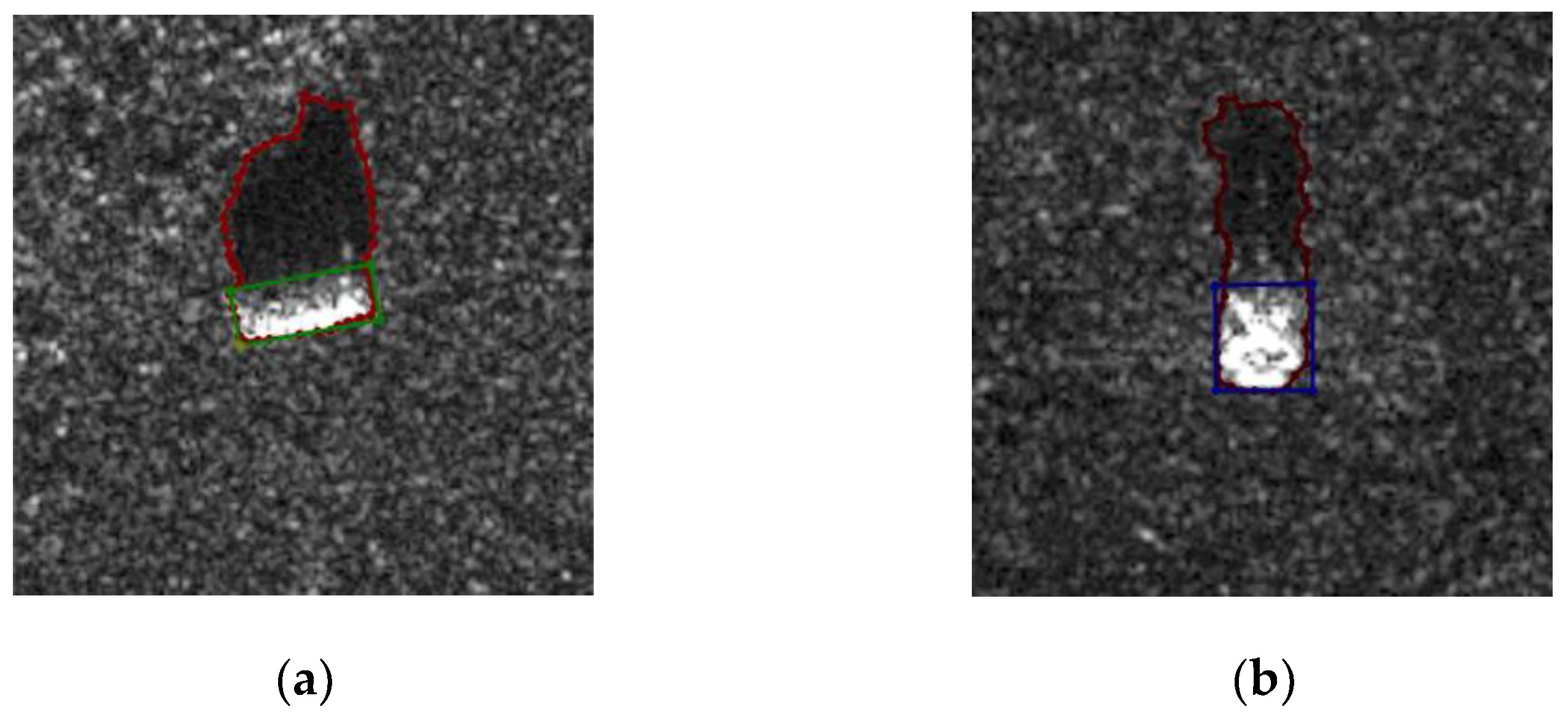
Figure 4.
(a) The pipeline of extracting grass and calculating the cosine similarity; (b) The histogram of the grass in Chips and Clutters.
Figure 4.
(a) The pipeline of extracting grass and calculating the cosine similarity; (b) The histogram of the grass in Chips and Clutters.
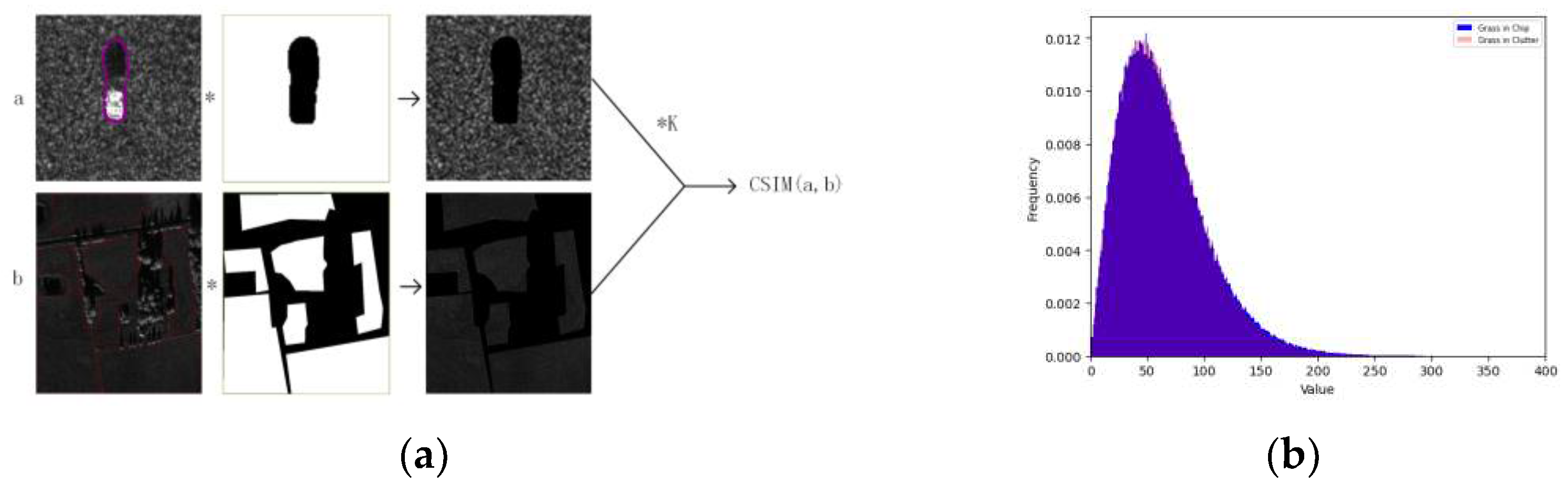
Figure 5.
A picture from the test set with 10346*1784 pixels (a) Densely ranked vehicles; (b) Sparsely ranked vehicles; (c) Town scene; (d) Field scene.
Figure 5.
A picture from the test set with 10346*1784 pixels (a) Densely ranked vehicles; (b) Sparsely ranked vehicles; (c) Town scene; (d) Field scene.
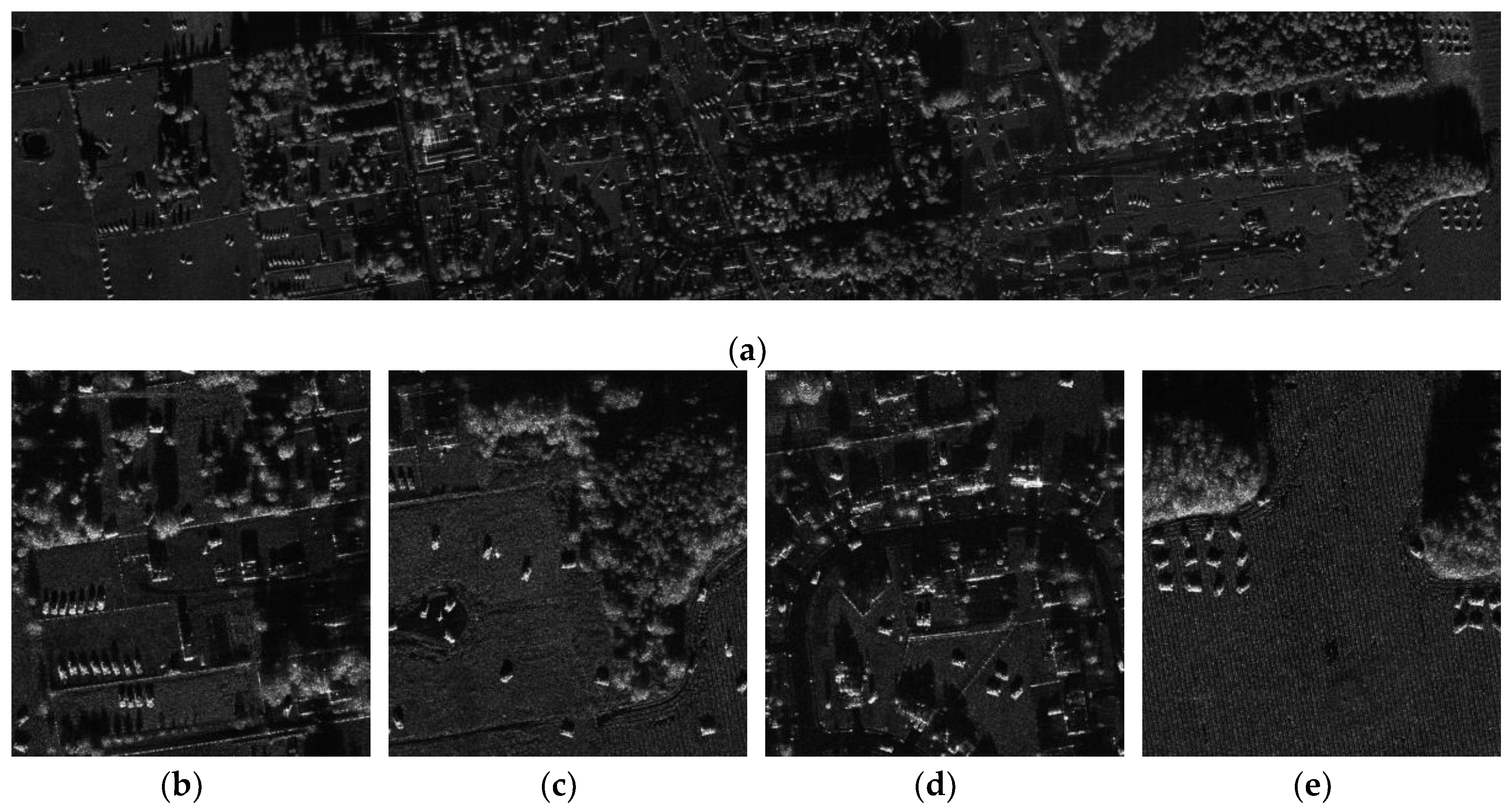
Figure 6.
Data statistics of Mix MSTAR (a) The area distribution of different categories of vehicles; (b) Histogram of number of annotated instances per image; (c) The number of vehicles in different azimuths; (d) The length - width distribution and aspect ratio distribution of vehicles.
Figure 6.
Data statistics of Mix MSTAR (a) The area distribution of different categories of vehicles; (b) Histogram of number of annotated instances per image; (c) The number of vehicles in different azimuths; (d) The length - width distribution and aspect ratio distribution of vehicles.
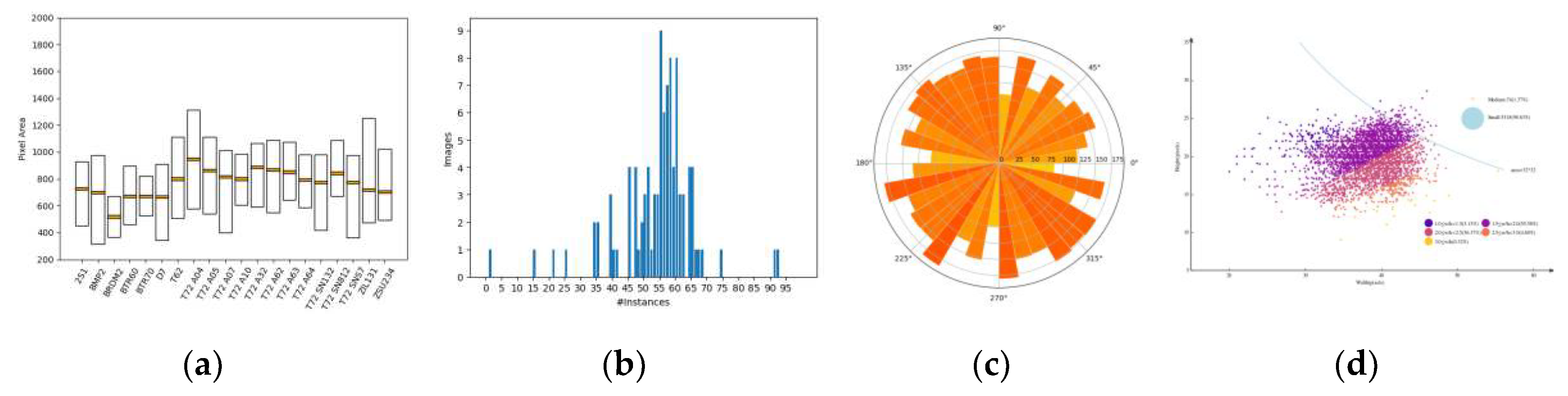
Figure 16.
(a) Confusion matrix of Oriented RepPoints on Mix MSTAR; (b) The P-R curves of models on Mix MSTAR.
Figure 16.
(a) Confusion matrix of Oriented RepPoints on Mix MSTAR; (b) The P-R curves of models on Mix MSTAR.
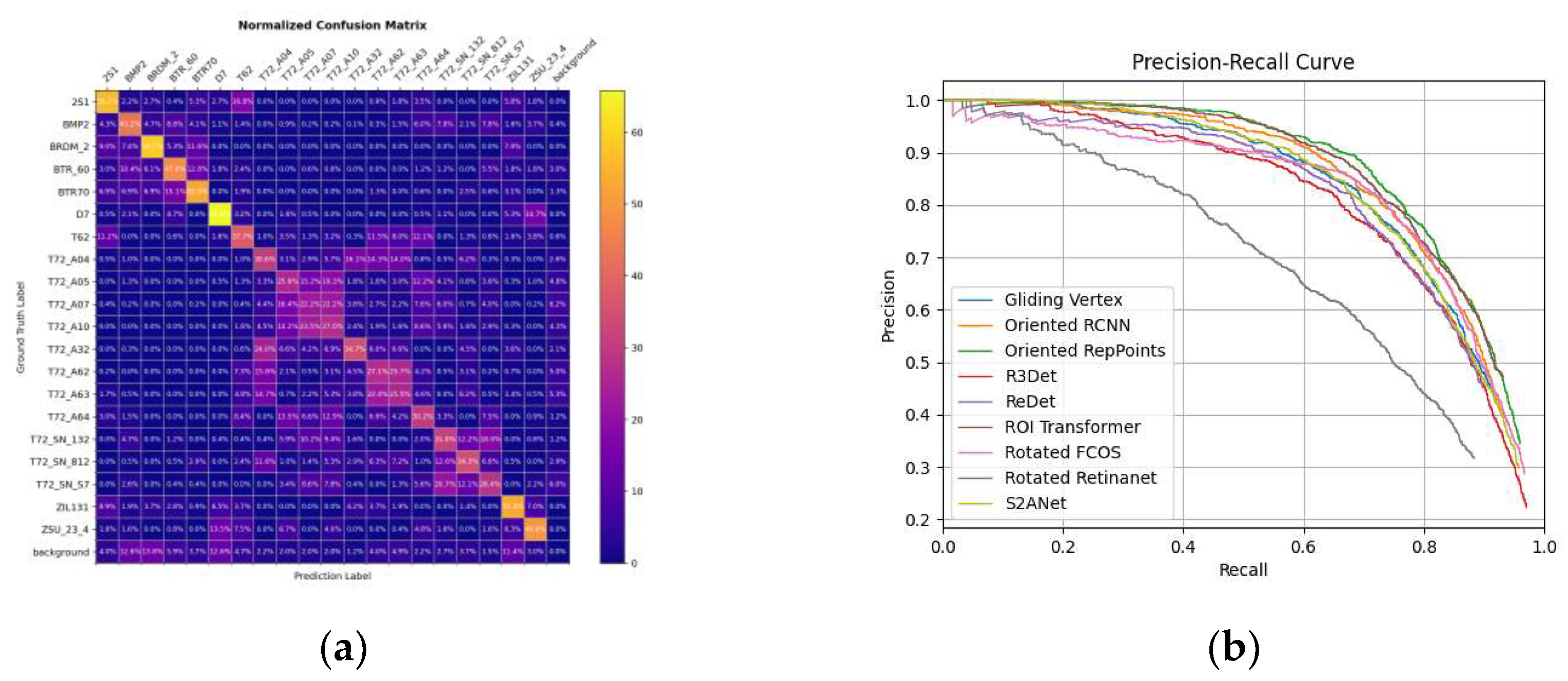
Figure 17.
Some detection result of different models on Mix MSTAR. (a) Ground truth; (b) Result of S2A-Net; (c) Result of ROI Transformer; (d) Result of Oriented RepPoints.
Figure 17.
Some detection result of different models on Mix MSTAR. (a) Ground truth; (b) Result of S2A-Net; (c) Result of ROI Transformer; (d) Result of Oriented RepPoints.
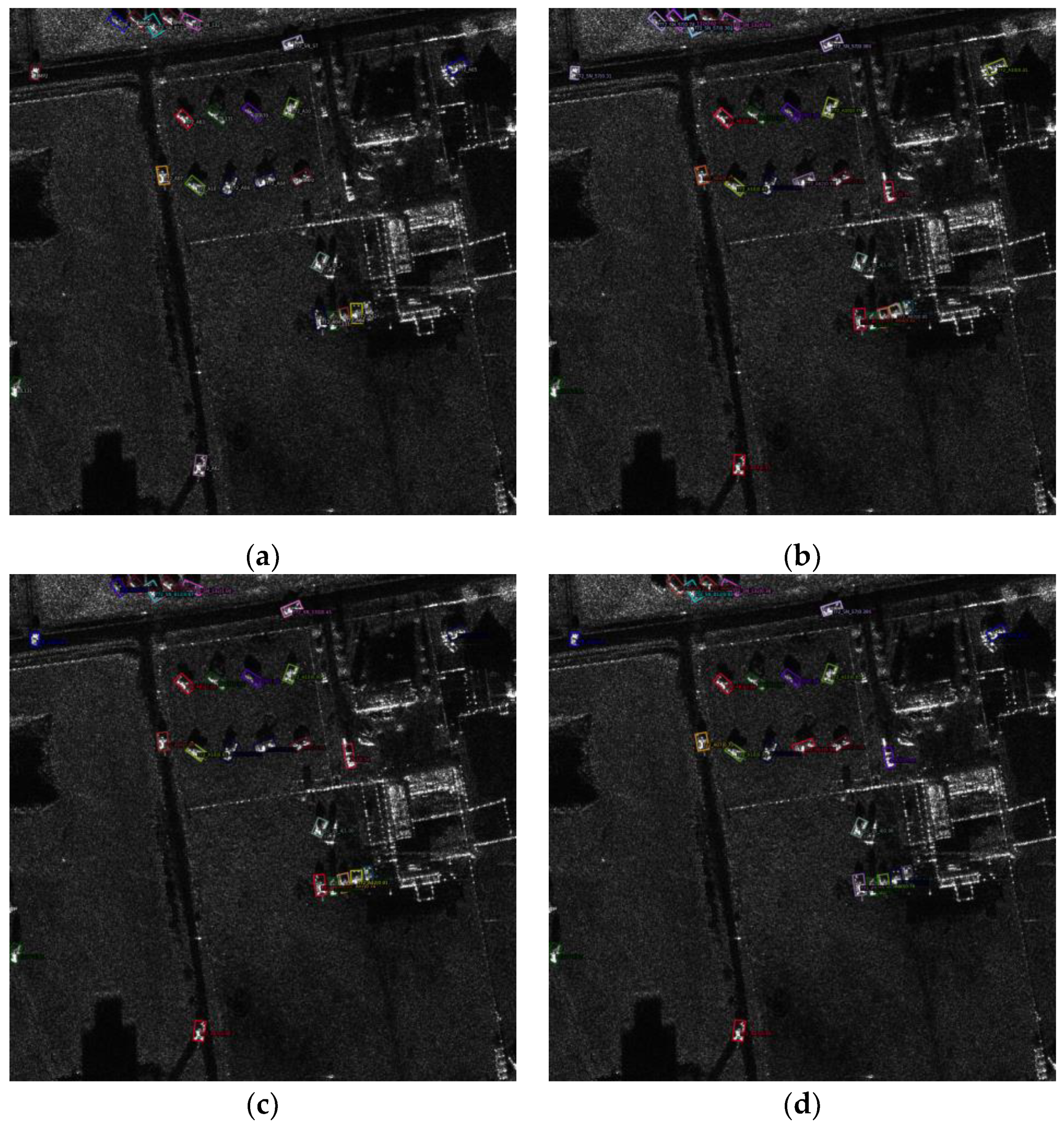
Figure 18.
(a) The result of ROI Transformer on concatenated Chips; (b) Class activation map of concatenated Chips.
Figure 18.
(a) The result of ROI Transformer on concatenated Chips; (b) Class activation map of concatenated Chips.
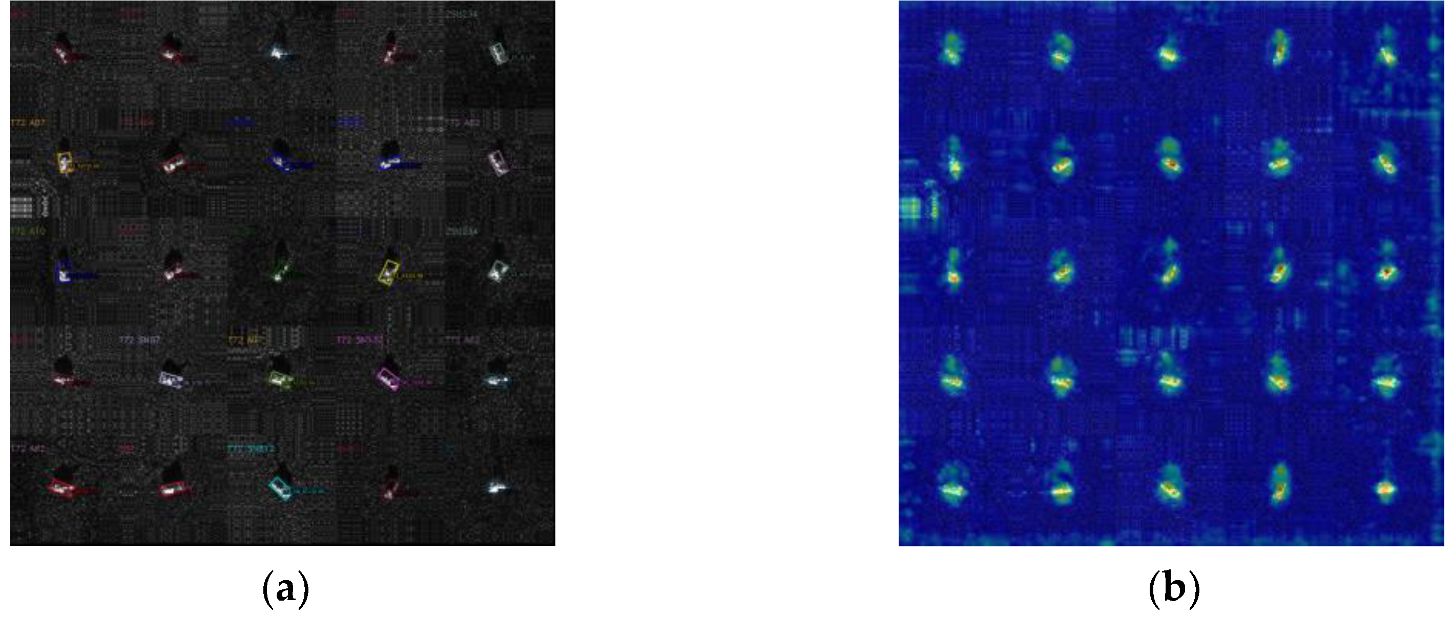
Figure 19.
(a) (c) T72 A05 Chips; (f) (g) T72 A07 Chips; (b) (d) Class activation map of T72 A05 Chips;(f) (h) Class activation map of T72 A07 Chips.
Figure 19.
(a) (c) T72 A05 Chips; (f) (g) T72 A07 Chips; (b) (d) Class activation map of T72 A05 Chips;(f) (h) Class activation map of T72 A07 Chips.
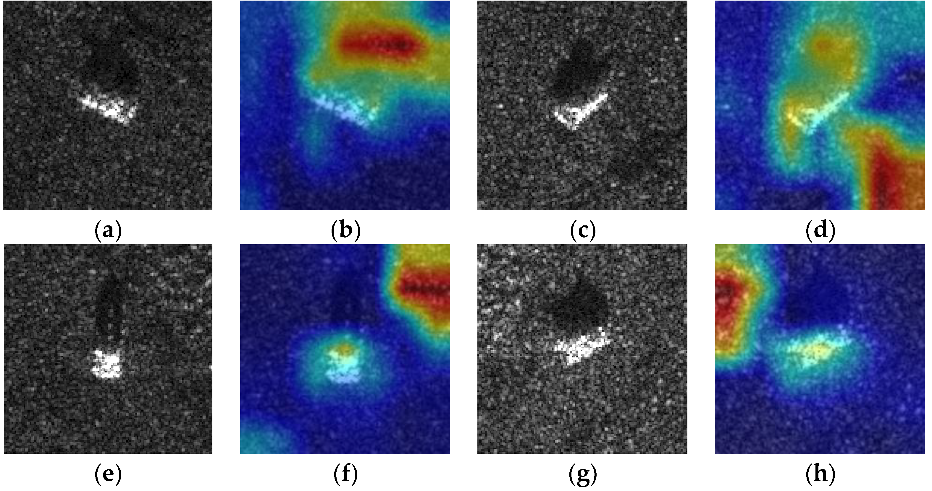
Figure 20.
The loss of pretrained/unpretrained models during training on Mini SAR. (a) Rotated Retinanet; (b) S2A-Net; (c) R3Det; (d) ROI Transformer; (e) Oriented RCNN; (f) ReDet; (g) Gliding Vertex; (h) Rotated FCOS; (i) Oriented RepPoints.
Figure 20.
The loss of pretrained/unpretrained models during training on Mini SAR. (a) Rotated Retinanet; (b) S2A-Net; (c) R3Det; (d) ROI Transformer; (e) Oriented RCNN; (f) ReDet; (g) Gliding Vertex; (h) Rotated FCOS; (i) Oriented RepPoints.
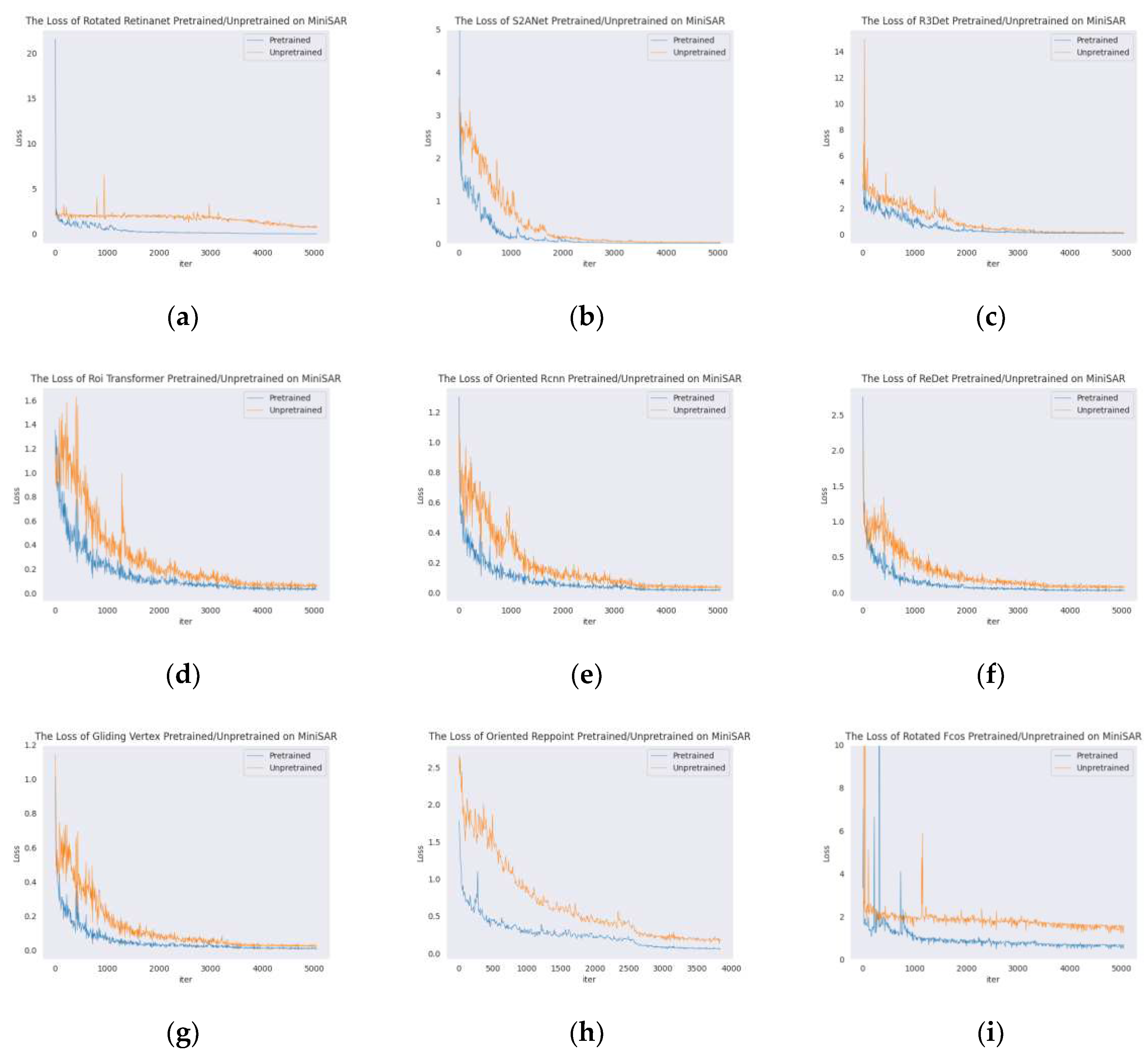
Figure 21.
The mAP of pretrained/unpretrained models during training on Mini SAR. (a) Rotated Retinanet; (b) S2A-Net; (c) R3Det; (d) ROI Transformer; (e) Oriented RCNN; (f) ReDet; (g) Gliding Vertex; (h) Rotated FCOS; (i) Oriented RepPoints.
Figure 21.
The mAP of pretrained/unpretrained models during training on Mini SAR. (a) Rotated Retinanet; (b) S2A-Net; (c) R3Det; (d) ROI Transformer; (e) Oriented RCNN; (f) ReDet; (g) Gliding Vertex; (h) Rotated FCOS; (i) Oriented RepPoints.
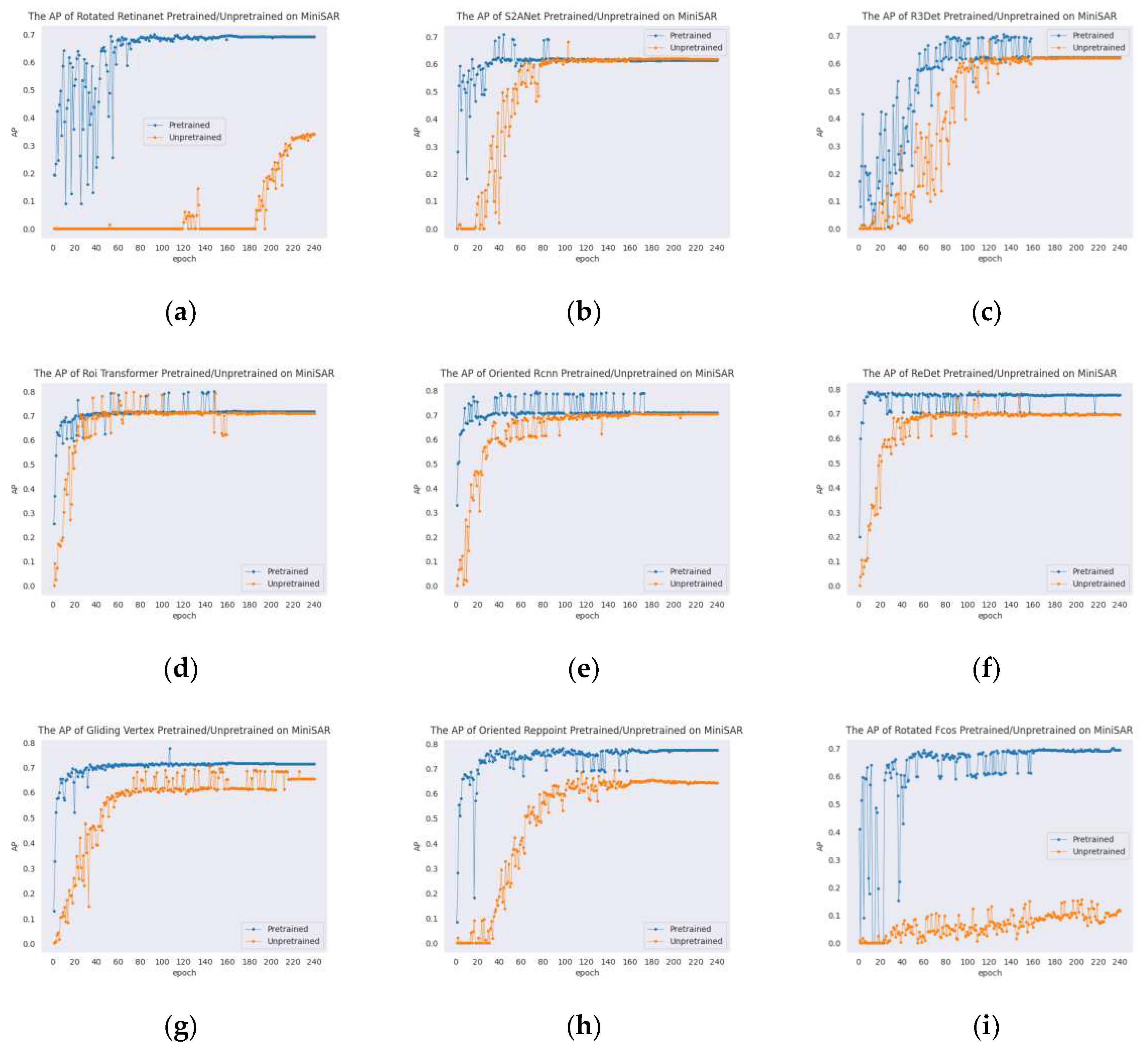
Figure 22.
Some detection result of Rotated Retinanet on Mini SAR. (a) Ground truth; (b) Rotated Retinanet trained on Mini SAR only; (c) Rotated Retinanet pretrained on Mix MSTAR; (d) Rotated Retinanet train on Mini SAR and Mix MSTAR.
Figure 22.
Some detection result of Rotated Retinanet on Mini SAR. (a) Ground truth; (b) Rotated Retinanet trained on Mini SAR only; (c) Rotated Retinanet pretrained on Mix MSTAR; (d) Rotated Retinanet train on Mini SAR and Mix MSTAR.
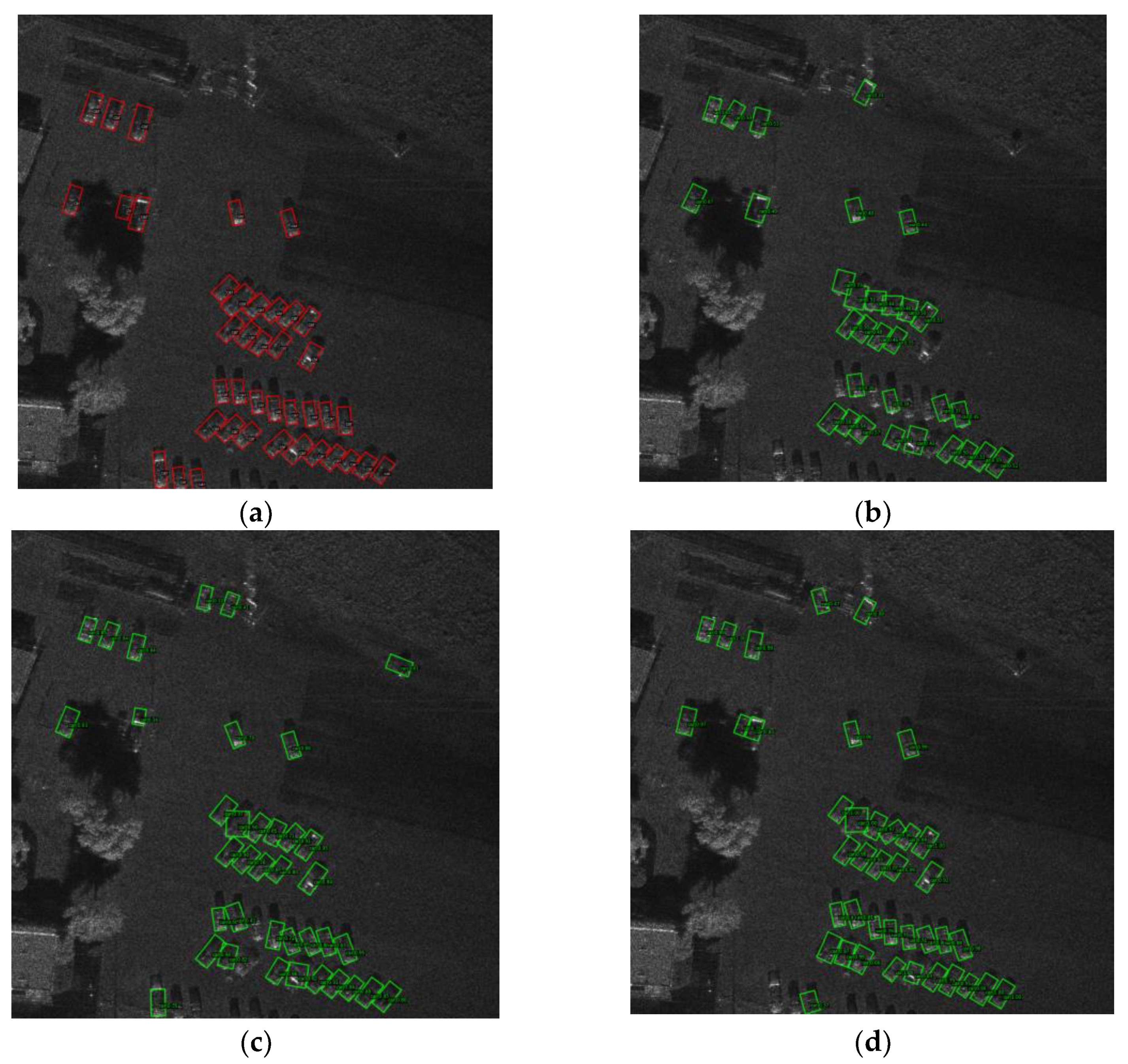
Figure 23.
The style transfer of optical and SAR by using CycleGAN. (a) A optical car image with label from DOTA domain; (b) Transferred image on Mix MSTAR domain.
Figure 23.
The style transfer of optical and SAR by using CycleGAN. (a) A optical car image with label from DOTA domain; (b) Transferred image on Mix MSTAR domain.
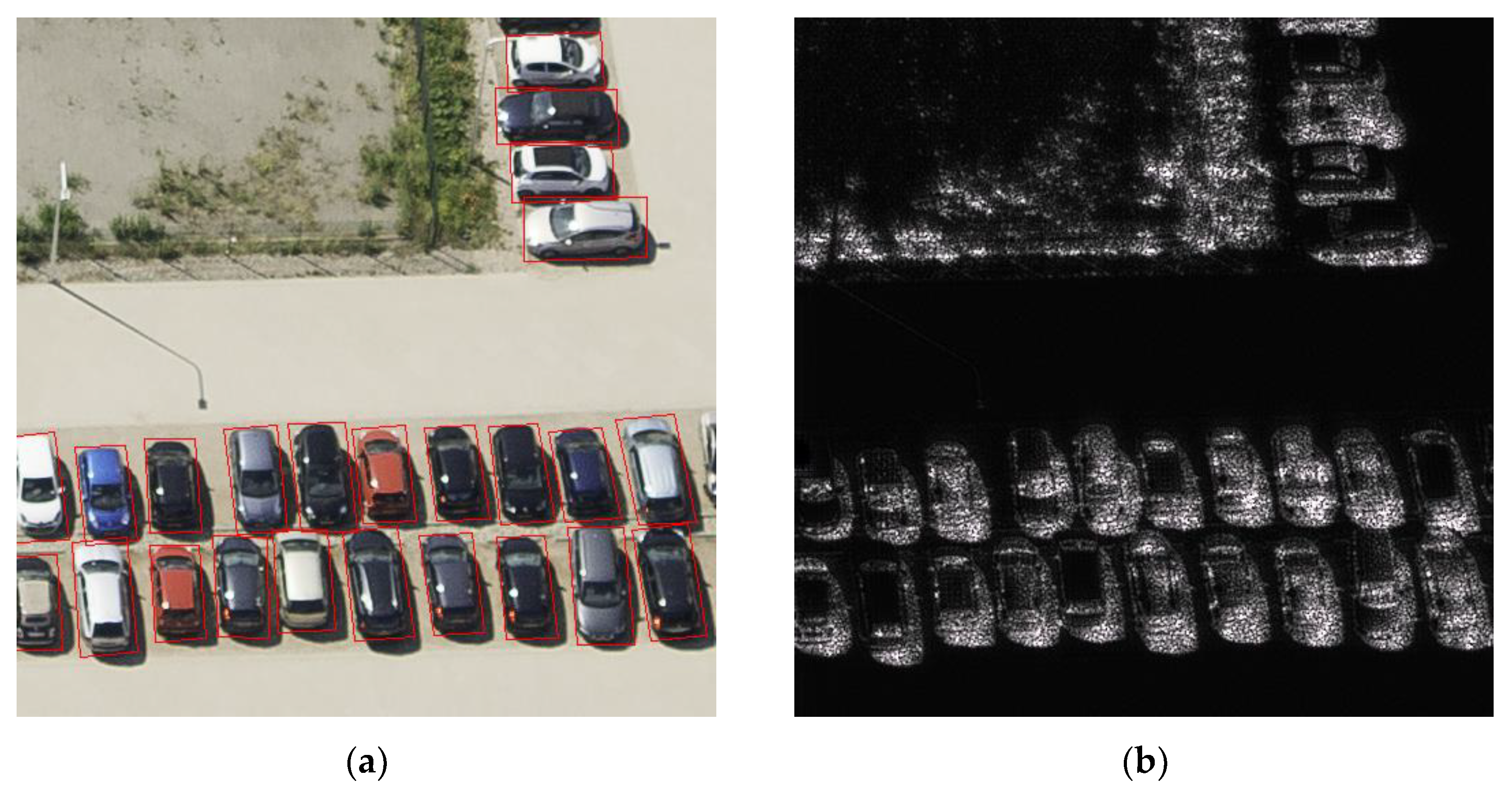
Figure 24.
Detection result of Redet on FARAD KA BAND. (a) Ground truth; (b) Result.
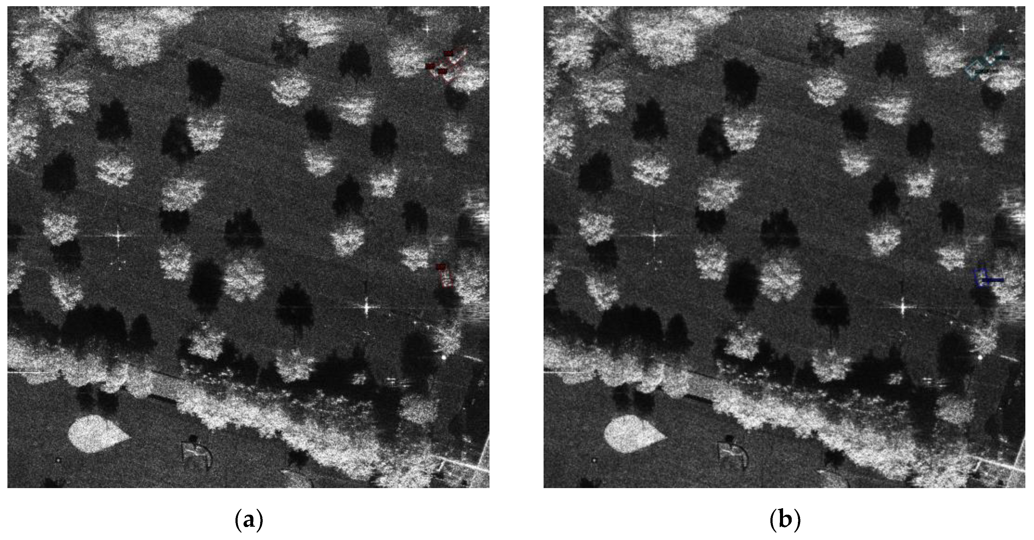

Table 1.
Detailed information of existing public SAR vehicle datasets with large scenes.
| Datasets | Resolution (m) | Image Size (pixel) | Images (n) | Vehicle Quantity | Noise Interference | |
|---|---|---|---|---|---|---|
| FARAD X BAND [13] | 0.1016*0.1016 | 1682*3334- 5736*4028 |
30 | Large | √ | |
| FARAD KA BAND [14] | 0.1016*0.1016 | 436*1288- 1624*4080 |
175 | Large | √ | |
| Spotlight SAR [15] | 0.1000*0.1000 | 3000*1754 | 64 | Small | × | |
| Mini SAR [16] | 0.1016*0.1016 | 2510*1638- 2510*3274 |
20 | Large | × | |
| MSTAR [10] | Clutters | 0.3047*0.3047 | 1472*1784- 1478*1784 |
100 | 0 | × |
| Chips | 0.3047*0.3047 | 128128- 192*193 |
20000 | Large | × | |
Table 2.
Basic radar parameter of Chips and Clutters in MSTAR.
| Collection Parameters | Chips | Clutters |
|---|---|---|
| Center Frequency | 9.60 GHz | 9.60 GHz |
| Bandwidth | 0.591 GHz | 0.591 GHz |
| Polarization | HH | HH |
| Depression | 15° | 15° |
| Resolution(m) | 0.3047*0.3047 | 0.3047*0.3047 |
| Pixel Spacing(m) | 0.202148*0.203125 | 0.202148*0.203125 |
| Platform | airborne | airborne |
| Radar Mode | spot light | strip map |
| Data type | float32 | uint16 |
Table 3.
Analysis of grassland data from Chips and Clutters in the same period.
| Grassland | Collection Date | Mean | Std | CV(std/mean) | CSIM |
|---|---|---|---|---|---|
| BMP2 SN9563 | 1995.09.01 - 1995.09.02 |
0.049305962 | 0.030280159 | 0.614127740 | 0.99826 |
| BMP2 SN9566 | 0.046989963 | 0.028360445 | 0.603542612 | 0.99966 | |
| BMP2 SN C21 | 0.046560729 | 0.02830699 | 0.607958479 | 0.99958 | |
| BTR70 SN C71 | 0.046856523 | 0.028143257 | 0.600626235 | 0.99970 | |
| T72 SN132 | 0.045960505 | 0.028047173 | 0.610245101 | 0.99935 | |
| T72 SN812 | 0.04546104 | 0.027559057 | 0.606212638 | 0.99911 | |
| T72 SNS7 | 0.041791245 | 0.025319219 | 0.605849838 | 0.99260 | |
| Clutters | 1995.09.05 | 63.2881255 | 37.850263 | 0.598062633 | 11 |
1 The CSIM of Clutters equal to 1 means compare themself.
Table 4.
Original imaging algorithm and improved imaging algorithm.
| Original imaging algorithm | Improved imaging algorithm |
|---|---|
| Input: Amplitude in MSTAR Data a>0, enhance=T or F | Input: Amplitude in MSTAR Data a>0, Threshold thresh |
| Output: uint8 image img | Output: uint8 image img |
| 1: fmin←min(a), fmax←max(a) | 1: for pixel∈a do |
| 2: frange←fmax-fmin, fscale←255/frange | 2: if pixel>thresh then |
| 3: a←(a-fmin)/fscale | 3: pixel←thresh |
| 4: img←uint8(a) | 4: scale←255/thresh |
| 5: if enhance then | 5: img←uint8(a/scale) |
| 6: hist8←hist(img) | 6: Return img |
| 7: maxPixelCountBin←index[max(hist8)] | |
| 8: minPixelCountBin←index[min(hist8)] | |
| 9: if minPixelCountBin>maxPixelCountBin then | |
| 10: thresh←minPixelCountBin-maxPixelCountBin | |
| 11: scaleAdj←255/thresh | |
| 12: img←img*scaleAdj | |
| 13: else | |
| 14: img←img*3 | |
| 15: img←uint8(img) | |
| 16: Return img |
Table 5.
The division of Mix MSTAR.
| Class | Train | Test | Total |
|---|---|---|---|
| 2S1 | 192 | 82 | 274 |
| BMP2 | 195 | 392 | 587 |
| BRDM2 | 192 | 82 | 274 |
| BTR60 | 136 | 59 | 195 |
| BTR70 | 137 | 59 | 196 |
| D7 | 192 | 82 | 274 |
| T62 | 191 | 82 | 273 |
| T72 A04 | 192 | 82 | 274 |
| T72 A05 | 192 | 82 | 274 |
| T72 A07 | 192 | 82 | 274 |
| T72 A10 | 190 | 81 | 271 |
| T72 A32 | 192 | 82 | 274 |
| T72 A62 | 192 | 82 | 274 |
| T72 A63 | 192 | 82 | 274 |
| T72 A64 | 192 | 82 | 274 |
| T72 SN132 | 137 | 59 | 196 |
| T72 SN812 | 136 | 59 | 195 |
| T72 SNS7 | 134 | 57 | 191 |
| ZIL131 | 192 | 82 | 274 |
| ZSU234 | 192 | 82 | 274 |
| Total | 3560 | 1832 | 5392 |
Table 6.
Performance Evaluation of models on Mix MSTAR.
| Category | Model | Params(M) | FLOPs(G) | FPS | mAP | Precision | Recall | F1-score |
|---|---|---|---|---|---|---|---|---|
| One-stage | Rotated Retinanet | 36.74 | 218.18 | 29.2 | 61.03±0.75 | 30.98 | 89.36 | 46.01 |
| Refine-stage | S2A-Net | 38.85 | 198.12 | 26.3 | 72.41±0.10 | 31.57 | 95.74 | 47.48 |
| R3Det | 37.52 | 235.19 | 26.1 | 70.87±0.31 | 22.28 | 97.11 | 36.24 | |
| Two-stage | ROI Transformer | 55.39 | 225.32 | 25.3 | 75.17±0.24 | 46.90 | 93.27 | 62.42 |
| Oriented RCNN | 41.37 | 211.44 | 26.5 | 73.72±0.45 | 38.24 | 93.56 | 54.29 | |
| ReDet | 31.7 | 54.48 | 18.4 | 70.27±0.75 | 45.83 | 89.99 | 60.73 | |
| Gliding Vertex | 41.37 | 211.31 | 28.5 | 71.81±0.19 | 44.17 | 91.78 | 59.64 | |
| Anchor-free | Rotated FCOS | 32.16 | 207.16 | 29.7 | 72.27±1.27 | 27.52 | 96.47 | 42.82 |
| Oriented RepPoints | 36.83 | 194.35 | 26.8 | 75.37±0.80 | 34.73 | 95.25 | 50.90 |
Table 7.
AP50 of each category on Mix MSTAR.
| Class | Rotated Retinanet | S2A-Net | R3Det | ROI Transformer |
Oriented RCNN | ReDet | Gliding Vertex | Rotated FCOS | Oriented RepPoints | Mean |
|---|---|---|---|---|---|---|---|---|---|---|
| 2S1 | 87.95 | 98.02 | 95.16 | 99.48 | 97.52 | 95.48 | 95.38 | 97.22 | 98.16 | 96.0 |
| BMP2 | 88.15 | 90.69 | 90.62 | 90.82 | 90.73 | 90.67 | 90.65 | 90.66 | 90.80 | 90.4 |
| BRDM2 | 90.86 | 99.65 | 98.83 | 99.62 | 99.03 | 98.14 | 98.39 | 99.72 | 99.22 | 98.2 |
| BTR60 | 71.86 | 88.52 | 88.07 | 88.02 | 85.67 | 88.84 | 86.18 | 86.55 | 86.54 | 85.6 |
| BTR70 | 89.03 | 98.06 | 95.36 | 97.57 | 97.68 | 92.53 | 97.02 | 96.67 | 95.06 | 95.4 |
| D7 | 89.76 | 90.75 | 93.38 | 98.02 | 95.70 | 93.42 | 95.51 | 95.52 | 96.21 | 94.3 |
| T62 | 78.46 | 88.66 | 91.20 | 90.29 | 92.39 | 86.53 | 89.70 | 89.99 | 90.20 | 88.6 |
| T72 A04 | 37.43 | 56.71 | 50.23 | 55.97 | 55.42 | 50.44 | 50.01 | 50.46 | 53.40 | 51.1 |
| T72 A05 | 31.09 | 40.71 | 43.10 | 46.17 | 48.27 | 44.56 | 45.93 | 42.09 | 50.04 | 43.5 |
| T72 A07 | 29.50 | 40.28 | 40.13 | 37.13 | 38.22 | 33.40 | 38.49 | 33.61 | 44.37 | 37.2 |
| T72 A10 | 27.99 | 39.82 | 36.00 | 40.71 | 36.81 | 34.04 | 34.44 | 40.67 | 47.57 | 37.6 |
| T72 A32 | 69.24 | 79.96 | 83.05 | 82.57 | 80.77 | 77.48 | 77.02 | 74.56 | 78.65 | 78.1 |
| T72 A62 | 41.06 | 49.49 | 50.05 | 54.32 | 47.31 | 41.97 | 45.71 | 53.77 | 54.00 | 48.6 |
| T72 A63 | 38.10 | 51.07 | 46.45 | 53.63 | 50.06 | 43.79 | 49.27 | 49.44 | 53.05 | 48.3 |
| T72 A64 | 35.51 | 58.28 | 57.54 | 67.37 | 66.65 | 57.95 | 63.38 | 58.47 | 66.14 | 59.0 |
| T72 SN132 | 34.18 | 54.95 | 45.71 | 59.85 | 58.16 | 56.80 | 52.23 | 54.35 | 65.38 | 53.5 |
| T72 SN812 | 49.27 | 72.01 | 61.86 | 77.42 | 74.23 | 65.13 | 71.34 | 73.33 | 72.14 | 68.5 |
| T72 SNS7 | 43.61 | 59.37 | 56.77 | 66.43 | 65.70 | 57.43 | 64.56 | 64.43 | 67.62 | 60.7 |
| ZIL131 | 96.06 | 96.24 | 97.76 | 99.00 | 97.88 | 98.78 | 96.16 | 95.24 | 99.58 | 97.4 |
| ZSU234 | 91.55 | 95.03 | 96.17 | 99.09 | 96.15 | 98.04 | 94.90 | 98.65 | 99.26 | 96.5 |
| mAP | 61.03 | 72.41 | 70.87 | 75.17 | 73.72 | 70.27 | 71.81 | 72.27 | 75.37 | 71.4 |
Table 8.
Best mAP of pretrained/unpretrained models on Mini SAR validation set.
| Model | Unpretrained | Pretrained |
|---|---|---|
| Rotated Retinanet | 38.00±15.52 | 71.40±0.75 |
| S2A-Net | 65.63±1.94 | 69.81±0.89 |
| R3Det | 66.30±2.66 | 70.35±0.18 |
| ROI Transformer | 79.42±0.61 | 80.12±0.01 |
| Oriented RCNN | 70.49±0.47 | 80.07±0.24 |
| ReDet | 79.47±0.58 | 79.64±0.31 |
| Gliding Vertex | 70.71±0.20 | 77.64±0.49 |
| Rotated FCOS | 10.82±3.94 | 74.93±2.60 |
| Oriented RepPoints | 72.72±2.04 | 79.02±0.39 |
Table 9.
mAP of pretrained/unpretrained/mixed trained models on Mini SAR.
| Model | Trained on Mini SAR only | Pretrained on Mix MSTAR | Add Mix MSTAR |
|---|---|---|---|
| Rotated Retinanet | 38.00±15.52 | 71.40±0.75 | 78.62±0.42 |
| Rotated FCOS | 10.82±3.94 | 74.93±2.60 | 77.70±0.10 |
Disclaimer/Publisher’s Note: The statements, opinions and data contained in all publications are solely those of the individual author(s) and contributor(s) and not of MDPI and/or the editor(s). MDPI and/or the editor(s) disclaim responsibility for any injury to people or property resulting from any ideas, methods, instructions or products referred to in the content. |
© 2023 by the authors. Licensee MDPI, Basel, Switzerland. This article is an open access article distributed under the terms and conditions of the Creative Commons Attribution (CC BY) license (http://creativecommons.org/licenses/by/4.0/).
Copyright: This open access article is published under a Creative Commons CC BY 4.0 license, which permit the free download, distribution, and reuse, provided that the author and preprint are cited in any reuse.


