
Submitted:
07 August 2023
Posted:
08 August 2023
You are already at the latest version
Abstract
Six mode shapes, including bending and torsion, were documented for five different basketball rims and backboards at the United States Military Academy, West Point, New York, USA. The frequency and damping ratio of each mode shape were also determined. The empirical process began with the time-domain excitation and response of each rim-backboard system. The impulse of excitation came from an impact hammer separately applied to sequentially, to each node. The sinusoidal response was gathered from an accelerometer at a fixed location, node 1. Each time-domain excitation-response was then converted to a frequency domain Bode plot for each node by a B&K 2034 Signal Analyzer, giving transfer functions of output/input versus frequency. Structural Measurements System (SMS) Software was used to fit mode shapes to the Bode plots. Each of the six mode shapes were fitted to the Bode plots of each node at a specific modal frequency. Each of the six mode shapes were a function of the locations of the nodes, and the Bode plot gathered at each node.
The first and second modes were critical for showing that the Energy Rebound Testing Device statistically correlated with the energy transferred to the rim and backboard. A known perturbation mass was selectively attached to the rim, to help isolate the dynamic masses and spring rates for the rim and backboard, to ascertain the kinetic energy transferred to the rim had a 95.67% inverse correlation with rim stiffness.
Keywords:
Basketball Rim and Backboard
; Modal Analysis
; Frequency
; Damping
1. Introduction
This research centered on the request by Dr. Jerry Krause, that the Department of Civil and Mechanical Engineering at the United States Military Academy at West Point, New York demonstrate whether the Fair-Court® Energy Rebound Testing Device was capable of detecting the stiffness of basketball rims. Although the authors all had a background in vibrations, none of us had ever studied basketball rims and backboards before. Thus, the first part of this study involved understanding the vibratory mode shapes of five basketball rims and backboards, with and without a shot-clock. Once this knowledge was gained, the basketball rim and backboard were treated as a two mass, two spring lumped-parameter model. Isolating the spring rates and masses of the rim and backboard was done via the use of a known perturbation mass applied to the outer end of the rim. The statistical correlation between energy absorbed reading from the ERTD and the spring rate of the rim concluded that the ERTD statistically correlated at R=95.67% with rim stiffness, and hence rim elasticity, over a 35.3% to 58.2% energy absorption range. Thus, we concluded that the ERTD was indeed a viable means of testing basketball rims and backboards, to help to add consistency to the physics of this sport.
2. Materials and Methods
The process diagram for the Structural Measurements System (SMS) Software is shown in Figure 1. This SMS software ran on a portable computer.
Each of the rim-backboard systems without a shot clock had the 38 nodes shown in Figure 2. The Cartesian coordinates of the 38 nodes were declared in Define Geometry and are listed in Table 1. The origin of the Cartesian coordinate system was the center of the circular rim, 381 mm (15 inches) from the backboard. The first 8 nodes were laid out counterclockwise, in an octagonal pattern, to document the 457 mm (18 inch) internal-diameter circular rim. The circular rim comprised a 15.9 mm (5/8 inch) diameter circular torus with a mass of 2.3 kg. The remaining 30 nodes documented the backboard. A steel bracket, defined by nodes 4-9-16-5, was used to attach the steel rim to the glass backboard. Layout of the grid on each actual rim and backboard was very tedious and usually took more time than the gathering of the excitation-response measurements. A large T-Square used in mechanical drawing proved very helpful.
The 38 nodes in Table 1 had to be properly sequenced to display the geometry shown in Figure 1. This sequencing, also done in Define Geometry, is shown in Table 2. The three columns of Line Numbers in Table 2 are in bold to make the line definitions in Table 2 easier to read. The action of lifting the pen, designated by an X, was done to avoid unwanted diagonal lines. Once Table 2 was completed, the rim-backboard shown in Figure 2 was displayed via Show Structures, Figure 1. As the rim-backboard was being assembled, Show Structures was periodically accessed to detect any mistakes before they pervasively propagated.
Once Define Structure was completed, the process went to Acquire Measurements, Figure 1. The instrumentation used in Acquire Measurements is shown in Figure 3. The 2644 line-driver charge-amplifiers were used to convert low level signals from the 8200 force transducer and the 4393 accelerometer. The 2644 charge amplifiers were always used together for both channel A (excitation) and channel B (response) when using the impact hammer. The orientation of the 2644 was critical. The externally threaded end of each 2644 had to be pointed towards the B&K 2034 analyzer or no measurements could be taken. Use of the 2644 was described by Serridge and Licht.
The B&K 8202 impact hammer (excitation) was used to individually gently tap each of the 38 nodes of Table 1 in succession. Rim nodes 1-8 were struck in the -Z direction and backboard nodes 9-38 were struck in the -X direction. The fixed location of the B&K 4393 accelerometer (response) was node 1, and the accelerometer was oriented in the vertical +Z direction as declared in New Project, Figure 1. The 4393 accelerometer was adhered to the rim via beeswax.
Table 3 shows six possible configurations of the 8202 impact hammer which could be used to adjust the frequency range of the excitation. Three tips were available: steel, plastic, and hard rubber. The softer the tip, the more the upper frequency of excitation was attenuated. Further reduction in the upper frequency of excitation could be achieved by adding an extra mass. For this study, the hard rubber tip and the extra mass were used, to limit the excitation to 0-340 Hz. We had no interest in vibrations in the kHz range, so we did not excite the rim-backboard system at that level. Additionally, we did not want any damage to the rim or backboard, perceived or actual, so use of the steel tip was never considered.
Use of the 8202 impact hammer was part art and part science. The goal was to impart a single-hit impulse at each node in Table 1. Then the response to the impulse at that node was measured by the 4393 accelerometer at node 1. It was critical that the impulse hammer never have a double-hit, as such a double-hit would have made impossible the gathering the desired output/input Bode plot. Thus, there was a certain amount of art in the wrist-action of the user, to impart a single-hit impulse that was not too severe yet not too soft. One subjective clue as to the adequacy of the application of the impact hammer was the low-frequency sound made by the rim-backboard. Thus, aural feedback was very important.
Table 4 gives the windowing and gains assigned to the 8202 impact hammer and the 4393 accelerometer
Once each of the 38 nodes were struck five times by the 8202 impact hammer, to average out noise, the excitation-response data gathered by the B&K 2034 Analyzer was stored as a *.FRF (Frequency Response Function) file in the portable computer by the SMS software. It was important to have a separate project for each rim-backboard, so that new *.FRF files for one project did not overlay previously measured *.FRF files for another project.
Figure 4 shows the magnitude versus frequency of a typical Bode plot of excitation/response. Near the bottom of Figure 4, rectangular windows were shown to be declared, per Table 4. At the bottom right corner of Figure 4, the settings of 1.01 mV/N for channel A (8202 impact hammer) and 318 µV/m/s2 for channel B (4393 accelerometer) are shown.
Once all of the Bode plots were calculated for the 38 nodes in Table 1, Structural Measurements System (SMS) Software was used to fit mode shapes to the Bode Plots using the polynomial method. To fit each mode shape, cursors were used to manually bracket clearly discernable peaks in a Bode plot, for the processing of a mode shape attributed to that peak in magnitude, such as shown in Figure 5.
Table 5 shows that there were six peaks of interest below 100 Hz for the rim-backboard without a shot-clock. We took advantage of the band option of the SMS software, which allowed the identification of multiple modes within one band. The approximate left and right cursor locations used to bracket each peak are listed in Table 5.
The six modes identified by use of Table 5 are shown in Figure 6, Figure 7, Figure 8, Figure 9, Figure 10 and Figure 11 for the case of a Hydra-Rib rim and backboard without a shot clock. Both vector and contour plots are shown for each mode shape to assist the reader. The first two modes of a Hydra-Rib with a shot clock are shown in Figure 12 and Figure 13. The modal frequency and damping are listed for each mode shape.
3. Results
The first two rim-backboard modes, Figure 6 and Figure 7, were equivalent to a two-mass, two-spring system. In Figure 6, the rim and backboard were in phase, thus representing the lowest modal frequency of 23.62 Hz. In Figure 7, the rim and backboard were 180o out of phase, thus increasing the modal frequency to 33.08 Hz. These two modes correspond exactly to the eigenvectors of a 2-spring, 2-mass system, as shown on the left of Figure 6 and Figure 7.
A lot was happening in Figure 8 and Figure 9. However, a first-order approximation is that modes 3 and 4 were influenced by the backboard plate bending as a simple plane. In Figure 8, the plane of the backboard was bending about the Z (vertical) axis. However, in Figure 9, the plane of the backboard was bending as the Y (horizontal) axis. Since the Y dimension of the backboard was 1.83 m, and the Z dimension was shorter at 1.22 m, per Table 6, the modal frequency of 41.54 Hz, in Figure 8, is lower than the modal frequency of 51.45 Hz, Figure 9. The circular rim (nodes 1-8) appeared to be hinging where it attached to the steel mount bracket (nodes 4-9-16-5).
Table 6 gives the parameters of the tempered glass used in each Hydra-Rib backboard. The length and width measurements of the rectangular tempered glass included a surrounding frame.
In Figure 10, the backboard flexed in a dome-like deformation along the X direction, at a higher frequency, 78.14 Hz. This dome-like deformation is somewhat similar to Irvine’s Figure 3, which also had an aspect ratio of 1.5:1. It also appeared to have its four corners constrained by the Hydra-Rib mount. The rim itself was now flexing in a more complicated mode shape.
Figure 11 exhibited the first torsion of the rim about the X-axis. This was at the highest modal frequency, 94.38 Hz, which we pursued.
The modal frequencies and damping ratios in Figure 6, Figure 7, Figure 8, Figure 9, Figure 10 and Figure 11 are summarized in the left frequency-damping data column of Table 7, below. All six modes of the rim-backboard were lightly damped, with the damping ratio ranging between 0.46% ≤ ζ ≤ 5.21%. Thus, the damped natural frequencies and the natural frequencies were essentially equal.
This study then included the Hydra-Rib basketball rim and backboard with a shot clock, as shown in Figure 12.
In Table 8, six additional nodes (49-54) were needed to add the shot clock and the steel bracket connecting the steel rim and glass backboard was augmented with two additional nodes (47-48). The rim (now nodes 1-16) was augmented with eight additional nodes to model the rim as a sixteen-sided hexadecagon (previously an octagon).
In Figure 12, there was simply not enough room to show all sixteen nodes comprising the circular rim. However, node 1, where the 4393 accelerometer was attached with beeswax, is shown at the very front end of the circular rim. Rim nodes 8 and 10 are also shown, because these six nodes 8-17-47-48-24-10 now comprise the steel bracket holding the steel rim (nodes 1-16) in place.
The 54 nodes in Table 8 had to be properly sequenced to display the geometry shown in Figure 12. This sequencing, also done in Define Geometry, is shown in Table 9. The three columns of Line Numbers in Table 9 are in bold to make the line definitions in Table 9 easier to read. The action of lifting the pen, designated by an X, was done to avoid unwanted diagonal lines. Once Table 9 was completed, the rim-backboard shown in Figure 12 was displayed via Show Structures, Figure 1. As the rim-backboard was being assembled, Show Structures was periodically accessed to detect any mistakes before they pervasively propagated.
Figure 13, above, shows the first and second modes of the Hydra-Rib with a shot clock. Analogous to the first two modes shown in Figure 6 and Figure 7, the two modes shown in Figure 13 were equivalent to a two-mass, two-spring system. In Figure 13, the rim and backboard were in phase for the first mode, thus representing the lowest modal frequency of 24.72 Hz. For the second mode in Figure 13. the rim and backboard were 180o out of phase, thus increasing the modal frequency to 29.93 Hz. This data is summarized in the right-most column of Table 7, above.
Once the first six modes of vibration were understood for the rim-backboard, the decision was made to focus on the first two modes, in order to isolate the rim stiffness by means of a perturbation mass MP hung from node 1, and compare that to the energy reading of the Energy Rebound Testing Device, ERTD. The ERTD used a dropped mass to measure the energy transferred to the rim.
The Fair-Court® Energy Rebound Testing Device (ERTD) mimicked dropping a basketball on the outer end of the rim. The ERTD used a 0.74 kg (26 ounce) drop-mass to approximate the mass of a basketball. The drop distance was 0.76 m (30 inches) to a compression spring. This compression spring caused the drop-mass to rebound. The ERTD was suspended from the end of the rim, as shown in Figure 14. The drop-mass was raised to a stop 0.76 m above the compression spring, then released. The drop-mass had two cylindrical portions, the smaller of which was black, and the larger 100 mm (dZ) long portion was shiny. The duration in time for the mass to drop and rebound (dt) was measured via a LM339N Quad Voltage Comparator. Thus, the drop and rebound velocities (dZ/dt) were both measured. From these velocities, the ratio of the change in kinetic energy (drop – rebound) of the drop-mass divided by the drop kinetic energy was expressed as a percentage.
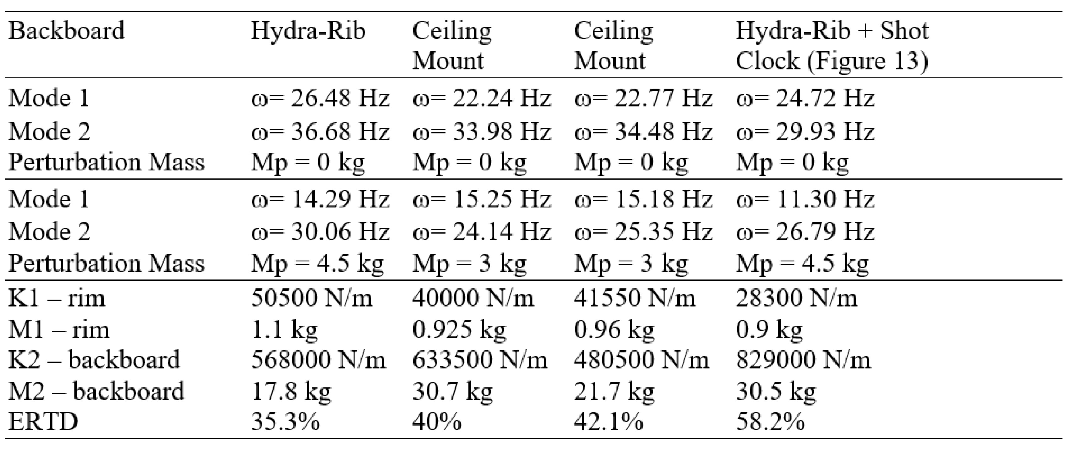
As shown in Figure 15, the first two modes of vibration were modeled as a two-spring, two-mass lumped parameter system. Masses M1 and M2 represented the dynamic masses and spring rates K1 and K2 represented the dynamic spring rate of the rim and backboard, respectively, at node 1, Figure 12. Determining K1, M1, K2, and M2 required four equations for these four unknowns. The quadratic characteristic equation used to determine the eigenvalues λ is shown in Figure 15. These eigenvalues were the square of the respective natural frequency in radians per second. The use of perturbation mass Mp provided two eigenvalue equations, and no perturbation mass (Mp=0) provided the additional two eigenvalue equations needed. Four natural frequencies, two modes with and without a perturbation mass Mp, were measured in Hertz via the modal analysis methods described above. These four natural frequencies were then converted to radians per second and squared, to obtain the four eigenvalues used in Figure 15 to calculate K1, M1, K2, and M2, Table 10.
ERTD readings for the four rim-backboards in Table 10 are also shown. The correlation =PEARSON function in Excel gave a cross-correlation coefficient of 95.67% in the inverse correlation between the reading of the Energy Rebound Testing Device and the rim spring rate (stiffness) K1, from the data listed in Table 10. The ERTD reading in percent versus rim spring rate K1 in kN/m is shown in Figure 16.
The least-squares equation for the ERTD reading, Figure 16, was:
ERTD % = 85.7368 – 1.04364*K1, where the spring rate of K1 was in kN/m.
Thus, the percentage reading of the ERTD increased as the K1 became softer, which is exactly what Dr. Krause hoped we would find. This meant that the ERTD was a portable and easy to use measure of rim stiffness and it could be used to provide more consistency to the sport of basketball.
4. Discussion and Conclusions
Article 4 of Section 15. Baskets-Ring of the 2022-2023 NCAA Men’s Basketball Rules Handbook states “All competitive rings shall be tested for rebound elasticity once before the season before the first date of competition and once before the postseason. The rebound elasticity requirement shall be 35% to 50% energy absorption and within a 5% differential between baskets on the same court.” Thus, the Energy Rebound Testing Device could help ensure that the rim (ring) spring rates were similar on both ends of the court, so that as teams switched ends during the basketball game, that the rims were consistent.
Funding
This research received no external funding.
Author Contributions:
Lieutenant Colonel (retired) Daniel J. Winarski, Army Reserves, mobilization designated to the Department of Civil and Mechanical Engineering, United States Military Academy at West Point. PhD, Mechanical Engineering, University of Michigan, 1976; MS, Mechanics, University of Colorado, 1973; BS, Mechanical Engineering, University of Michigan, 1970. USMA courses taught: EM-486 Vibration Engineering, EM-364 Mechanics of Materials, EM-302 Statics and Dynamics. IBM Tucson, Arizona: retired with more than 540 issued patents worldwide. Brigadier General (retired) Kip P. Nygren, Professor and Head, Department of Civil and Mechanical Engineering, United States Military Academy at West Point, New York 1995- 2007. PhD, Aerospace Engineering, Georgia Tech, 1986; MS, Aeronautical & Astronautical Engineering, Stanford University, 1978; BS, United States Military Academy, 1969. USMA courses taught: ME-362 Fluid Mechanics, ME-401 Introduction to Mechanical Engineering Design, ME-489 Advanced Individual Study, ME-471 Dynamic Modeling and Control, EM-486 Vibration Engineering, ME-302 Statics and Dynamics, EM-301 Thermodynamics, ME-483 Aerospace Systems Design, ME-481 Aircraft Performance & Static Stability, ME-488, Aircraft Flight Dynamics, ME-388 Helicopter Aeronautics, and ME-387 Introduction to Aerodynamics. Published papers and presentations in the areas of dynamics of structures, engineering education, energy systems and history of technology. Tyson Y. Winarski: Professor of Practice of Intellectual Property, Sandra Day O’Connor College of Law, Arizona State University. MS, Electrical Engineering, Arizona State University, 2001; Juris Doctorate, Arizona State University, 1998; BS, Mechanical Engineering, University of Colorado, 1995. In addition to several published articles, his resume includes fifty issued patents in the areas of nanotechnology, artificial intelligence, and blockchain. He is concluding six years on the board of directors of the Grand Canyon Conservancy. He is also a member of the Arizona Bar and the California Bar.
Acknowledgments
This paper is dedicated to and in memory of Dr. Jerry Krause, who was Director of Men's Basketball Operations, Gonzaga University. He also served a 5-year civilian term at the U.S. Military Academy at West Point, where he was Professor of sport philosophy, and Director of Instruction for the department of physical education. Dr. Krause was a long-standing member of the NCAA Rules Committee, was on the Board of Directors of the National Association of Basketball Coaches and served on the Selection Committee of the National Basketball Hall of Fame. He was also a member of the NAIA Basketball Coaches and National Association for Sports and Physical Education Halls of Fame. His Bachelor's degree was from Wayne State University in 1959; Master's degree in 1965 and Doctorate degree in 1967, both from Northern Colorado. Dr. Krause had authored many books on coaching basketball, produced many instructional videos, and served as a consultant to many athletic organizations. It was Dr. Krause who inspired and supported this study.
Conflicts of Interest
The authors declare no conflict of interest.
References
- “Assembly, Operation & Maintenance Manual: Fair-Court® Official Basketball Equipment Testing System, No. ERTD2003NCAA.” Copyright 2003 by the Porter Athletic Equipment Company. Available online: https://cdn.arenacommerce.com/basketballproductsinternational/Porter%20Fair-Court%20Rim%20Testing%20System_090109030803-fair-court-instructions.pdf.
- “Product Data: Piezoelectric Charge Accelerometer Types 4393 and 4393-V.” Copyright 2018-08 by Brüel & Kjaer. Available online: https://www.bksv.com/media/doc/bp2043.pdf and https://www.bksv.com/en/transducers/vibration/accelerometers/charge/4393.
- “Technical Documentation: Impact Hammer Type 8202.” Copyright May, 1993 by Brüel & Kjaer, Available online: https://media.hbkworld.com/m/7a8ee3f9bea9db2b/original/Impact-Hammer-Type-8202.pdf.
- Serridge, Mark and Licht, Torben. “Piezoelectric Accelerometers and Vibration Preamplifiers: Theory and Application Handbook.” November, 1987. Available online: https://www.bksv.com/media/doc/bb0694.pdf.
- Irvine, Tom. “The Natural Frequency of a Rectangular Plate Point-Supported at each Corner, Revision C.” August 1, 2011. Available online: http://www.vibrationdata.com/tutorials2/plate_point_corner.pdf.
- 2022-2023 NCAA Men’s Basketball Rules Handbook, updated November 7, 2022. Manuscript Prepared By: Art Hyland, Secretary-Rules Editor, NCAA Men’s Basketball Rules Committee. Edited By: Andy Supergan, Assistant Director of Playing Rules and Officiating. Available online: http://www.ncaapublications.com/productdownloads/BK23-20221107.pdf.
Figure 1.
Process Diagram for SMS Software.
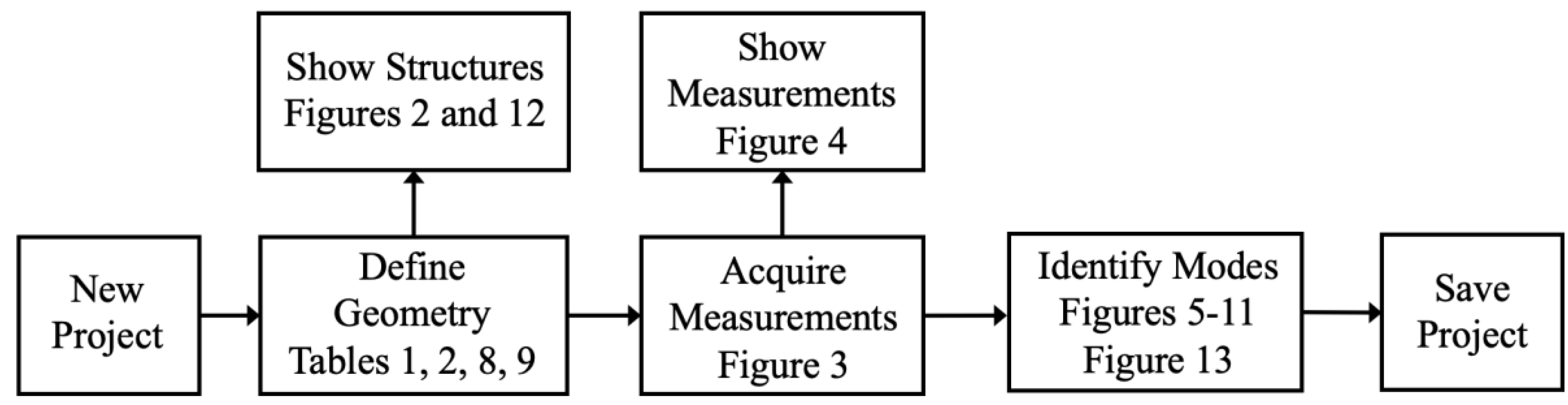
Figure 2.
Layout of 38 rim-backboard nodes.
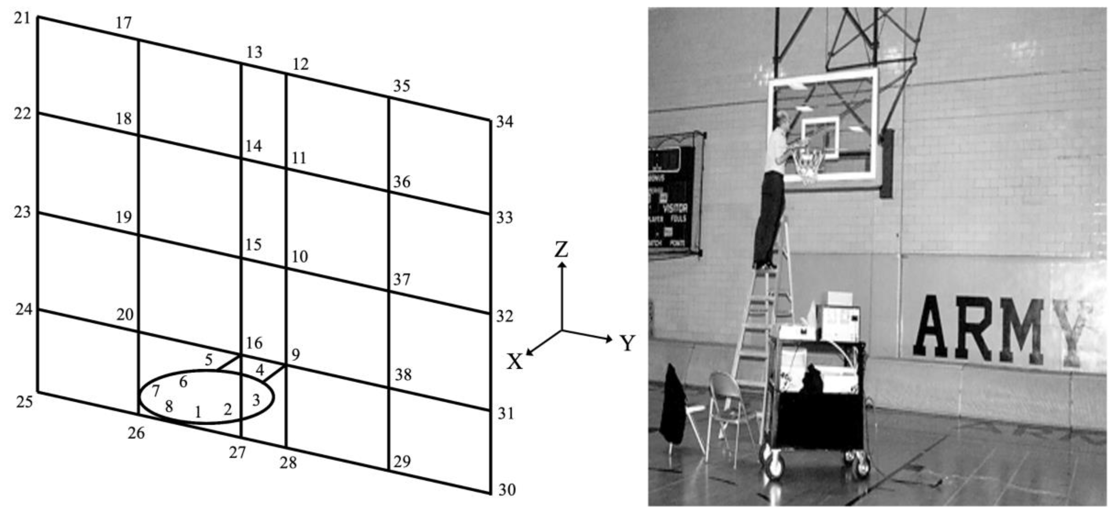
Figure 3.
8202 Impact Hammer and 4393 Accelerometer Instrumentation.
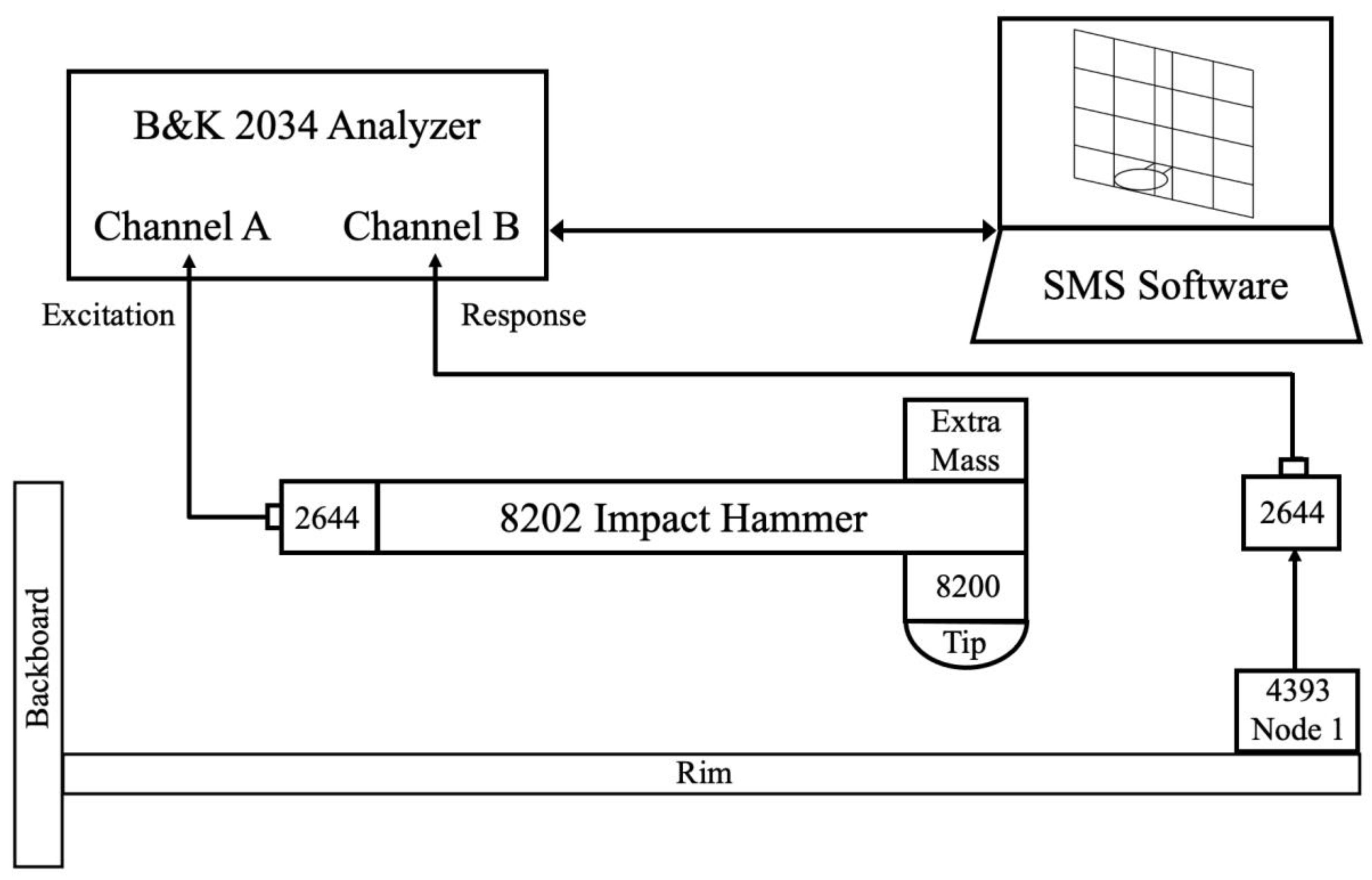
Figure 4.
Magnitude versus Frequency of a Typical Bode Plot of Excitation/Response.
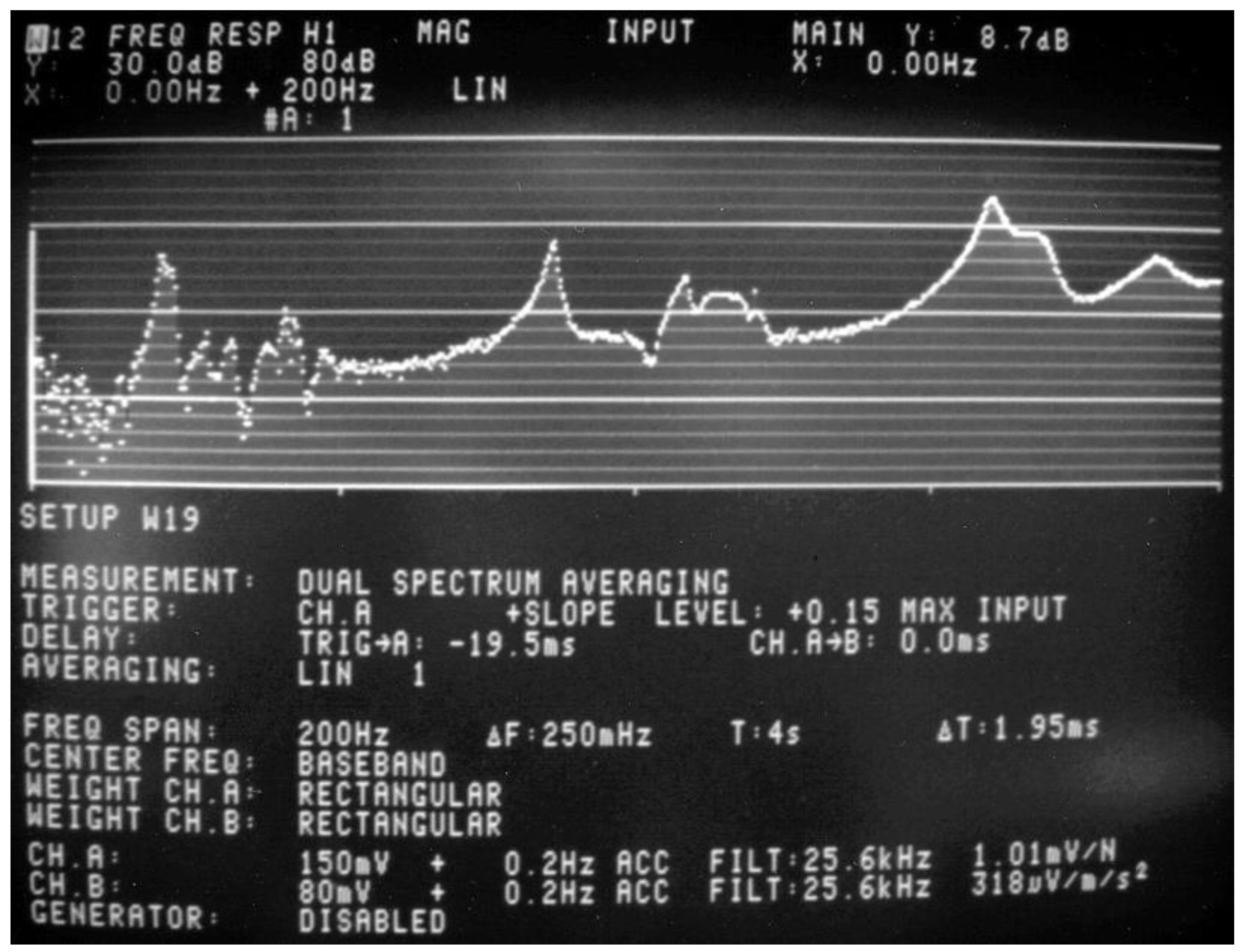
Figure 5.
Example of Manually Bracketing a Peak of Interest with Left and Right Cursors.
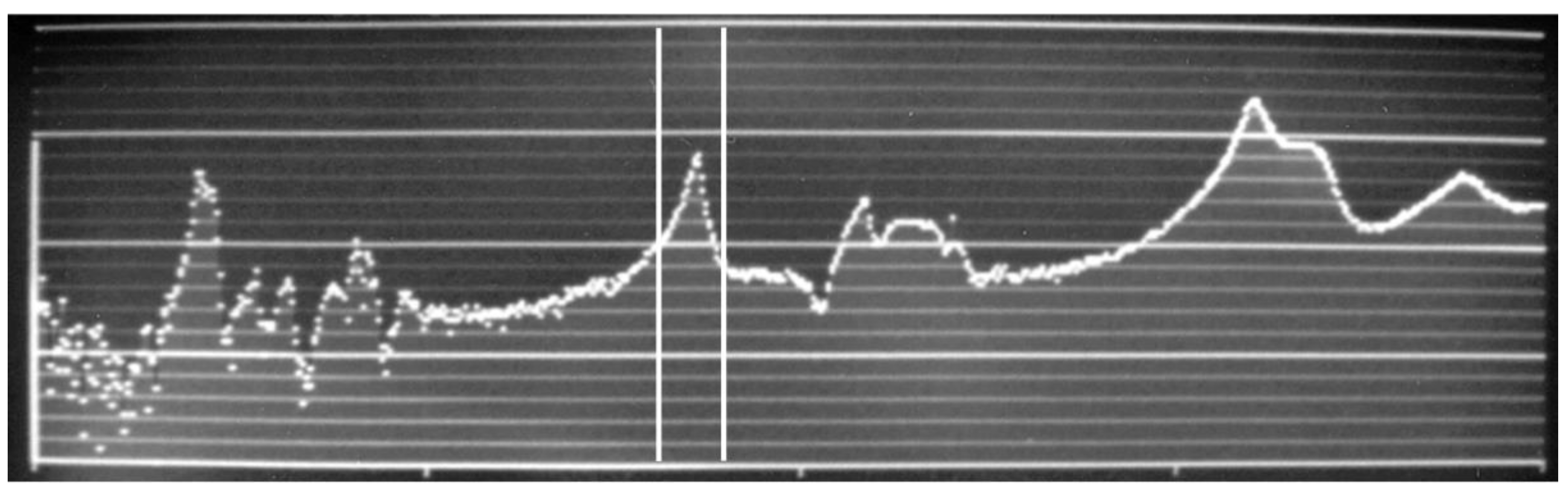
Figure 6.
Mode-1: ω = 23.62 Hz, Damping Ratio ζ = 2.66%.
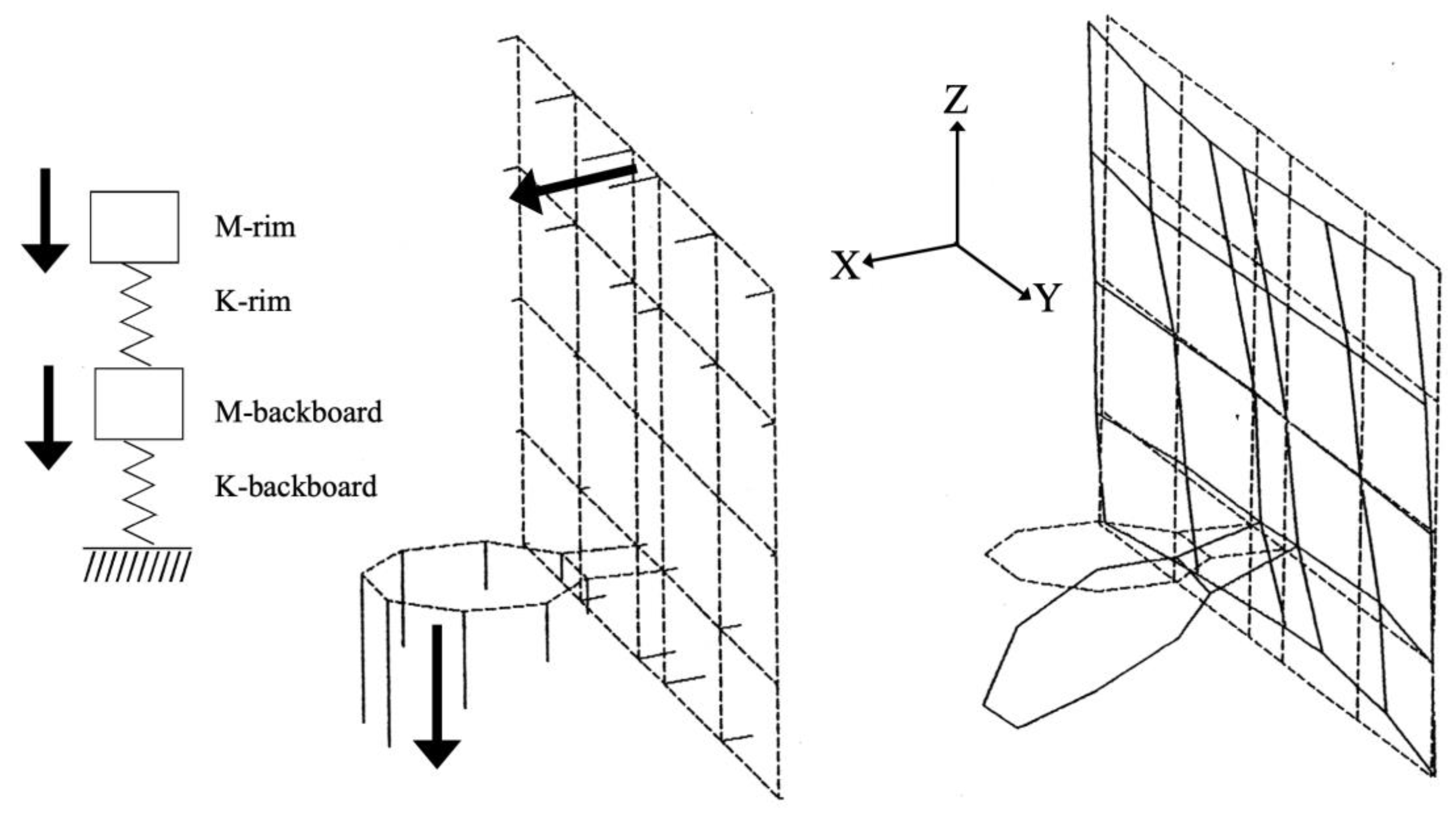
Figure 7.
Mode-2: ω = 33.08 Hz, Damping Ratio ζ = 2.55%.
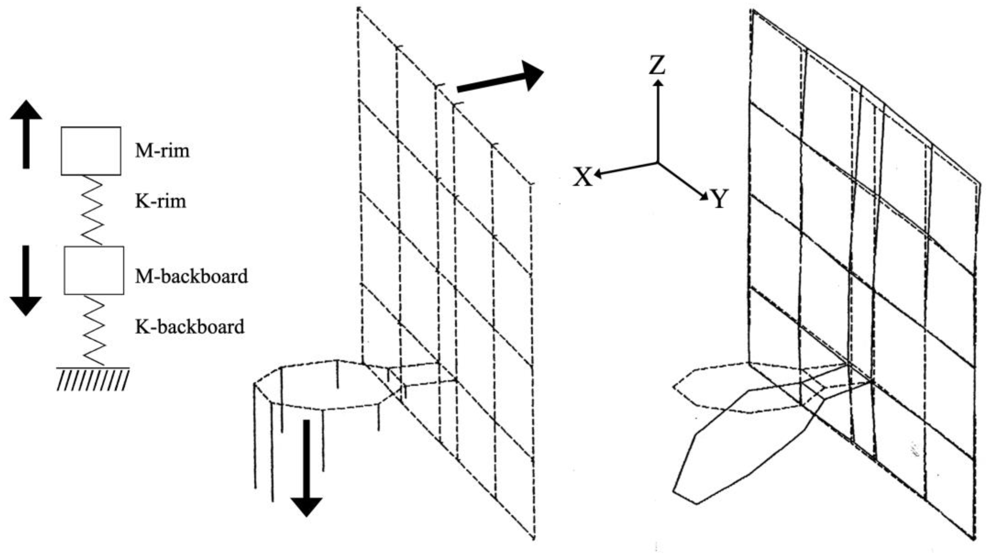
Figure 8.
Mode-3: ω = 41.54 Hz, Damping Ratio ζ = 3.69%.
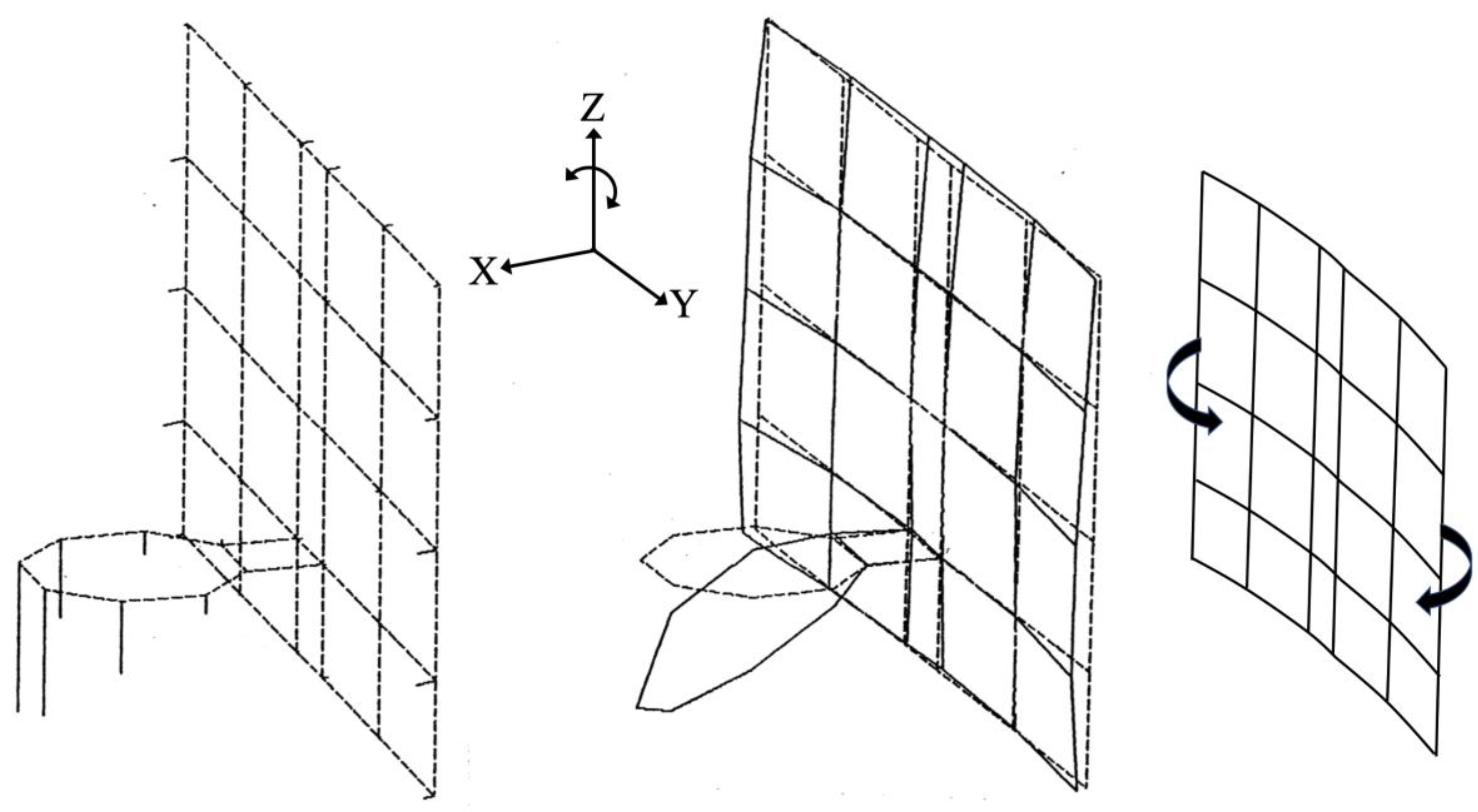
Figure 9.
Mode-4: ω = 51.45 Hz, Damping Ratio ζ = 1.31%.
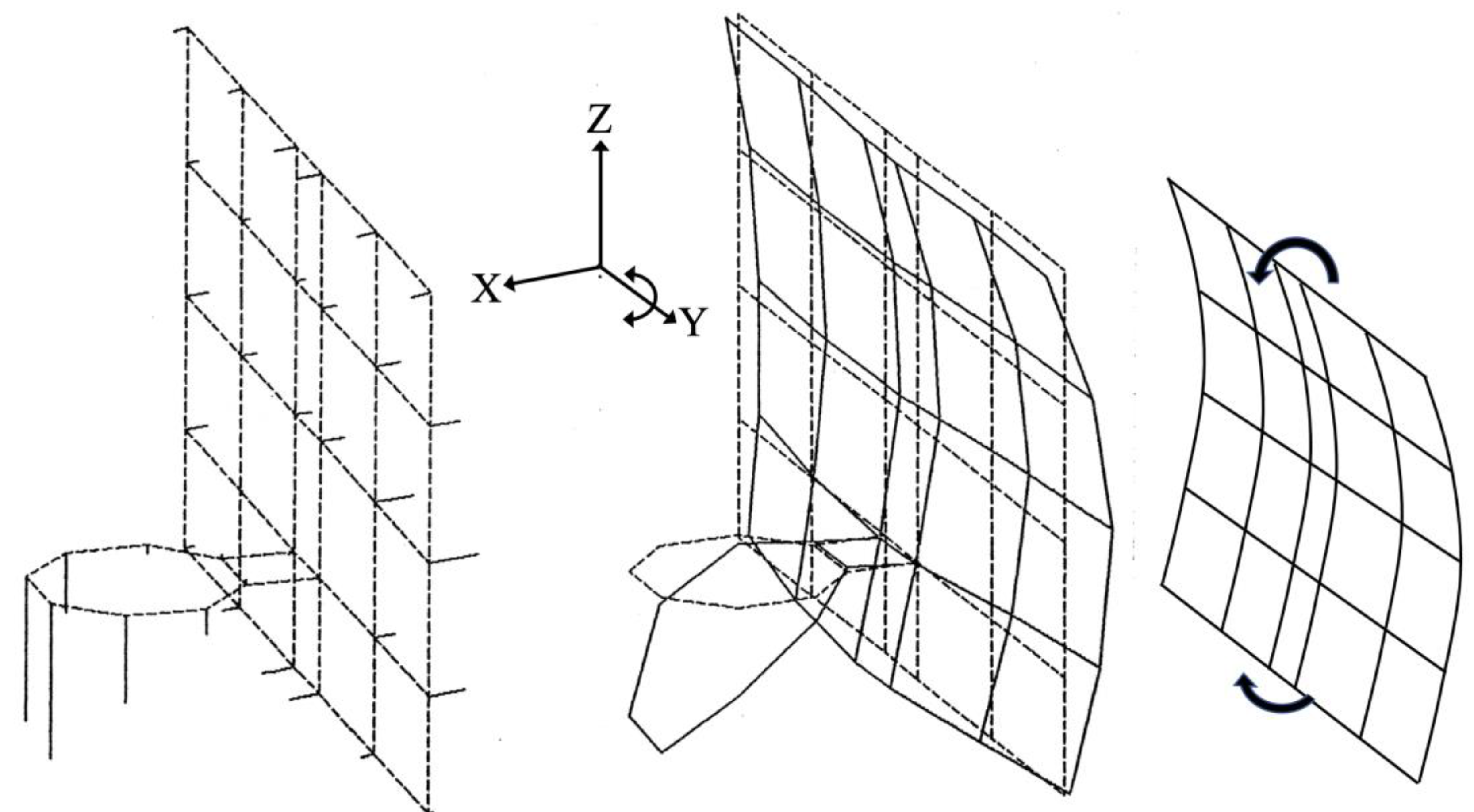
Figure 10.
Mode-5: ω = 78.14 Hz, Damping Ratio ζ = 1.46%.
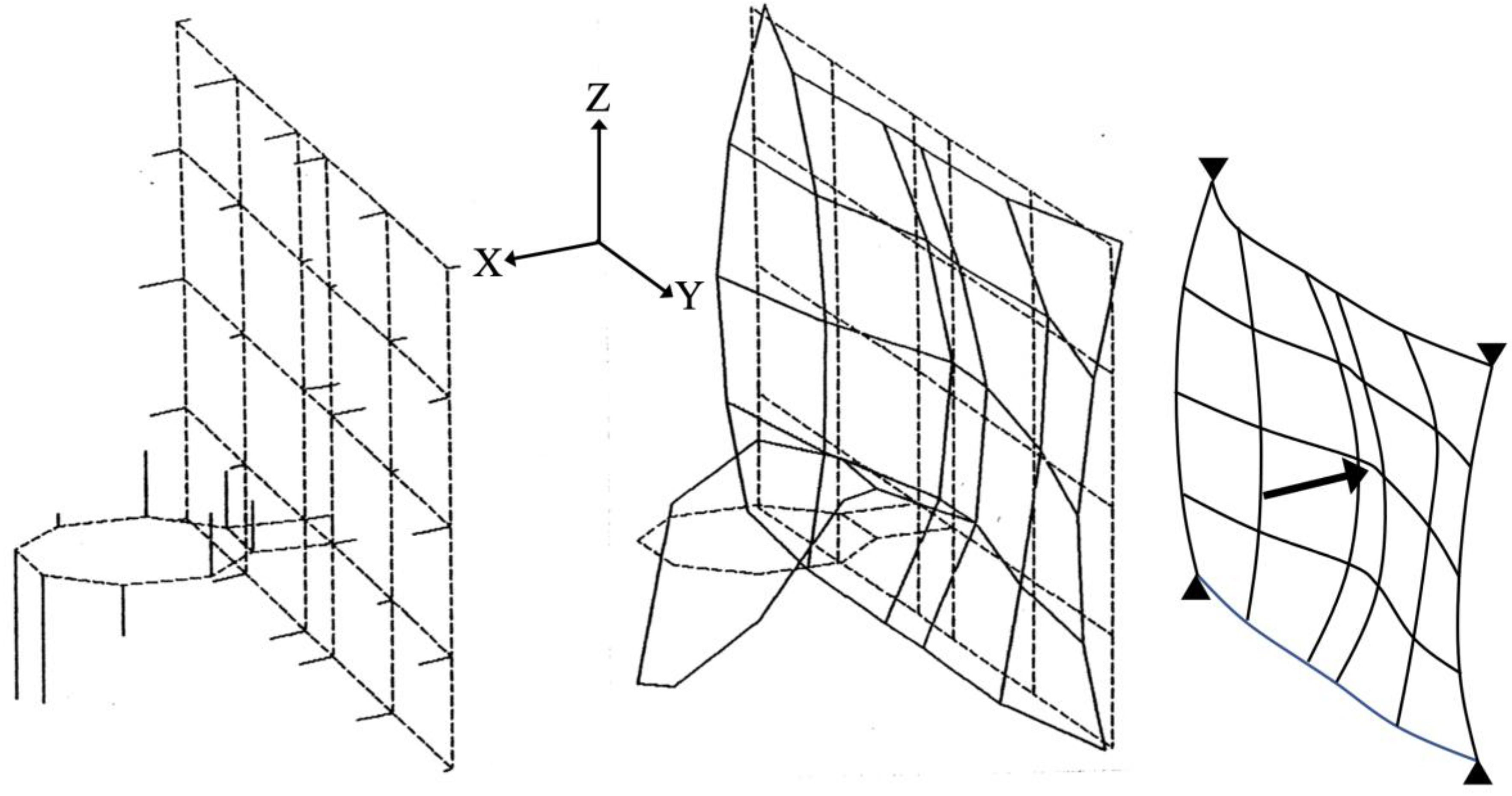
Figure 11.
Mode-6: ω = 94.38 Hz, Damping Ratio ζ = 2.85%.
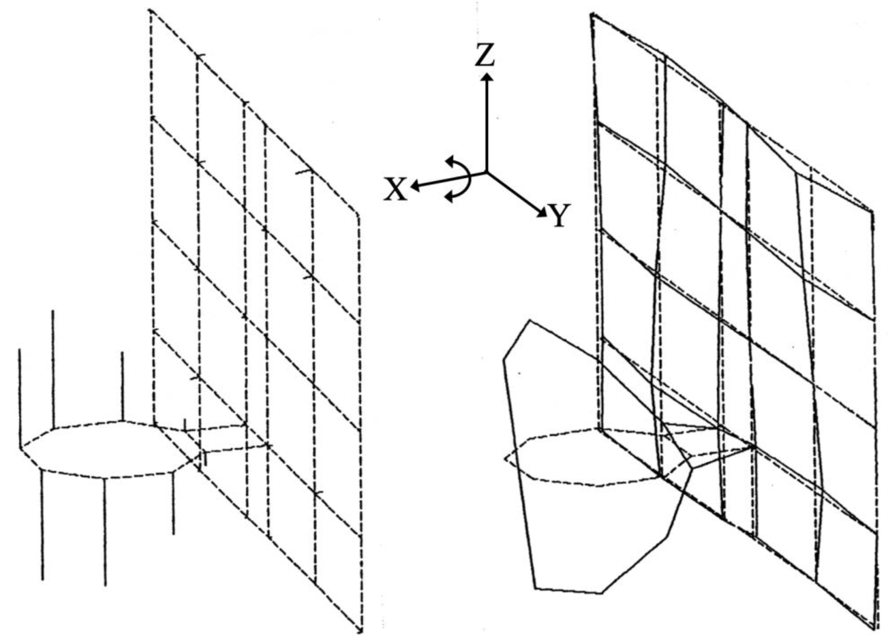
Figure 12.
Hydra-Rib Basketball Rim and Backboard with a Shot Clock.
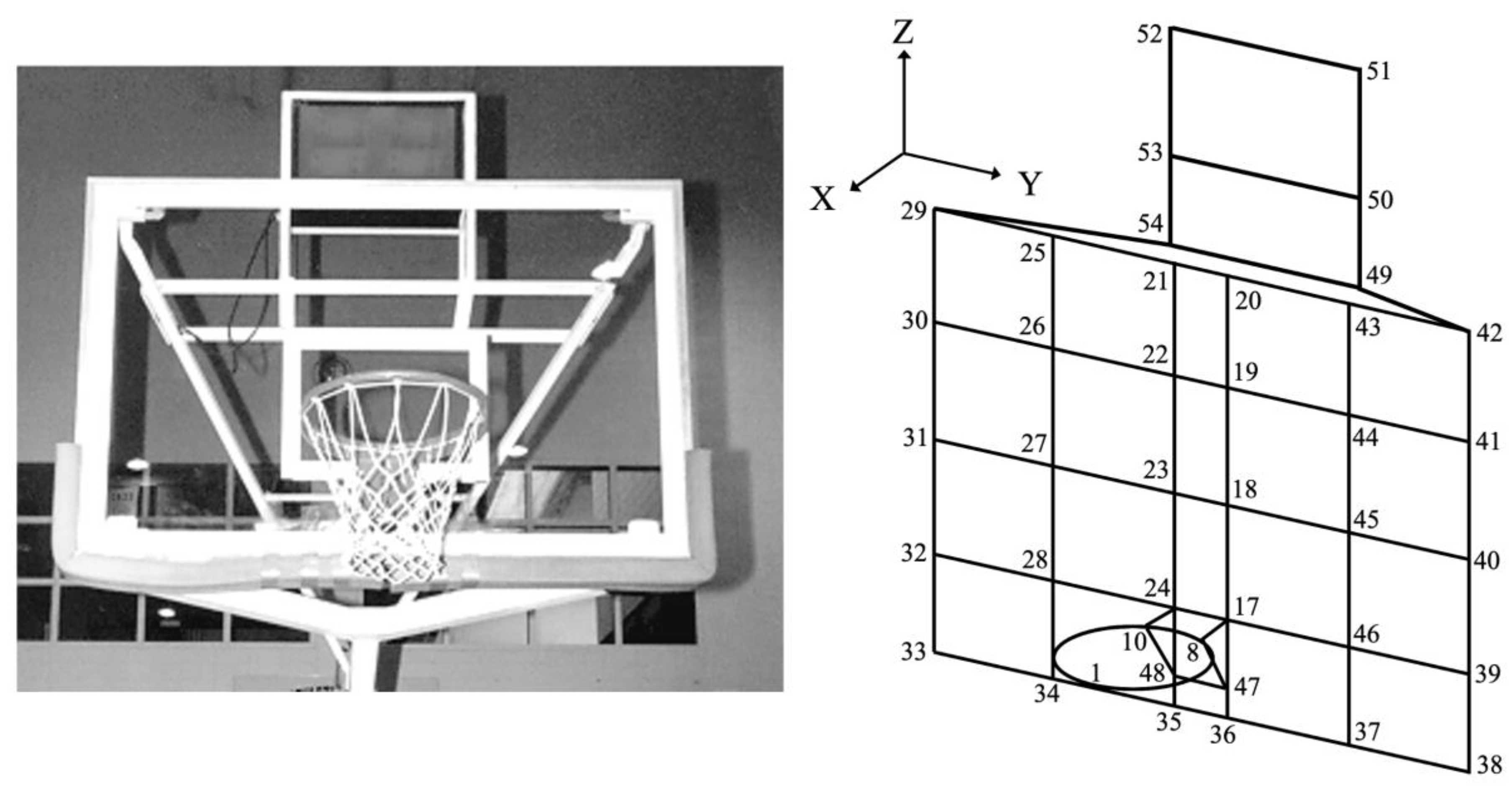
Figure 13.
Hydra-Rib with Shot Clock: Mode 1 (24.72 Hz) and Mode 2 (29.93 Hz).
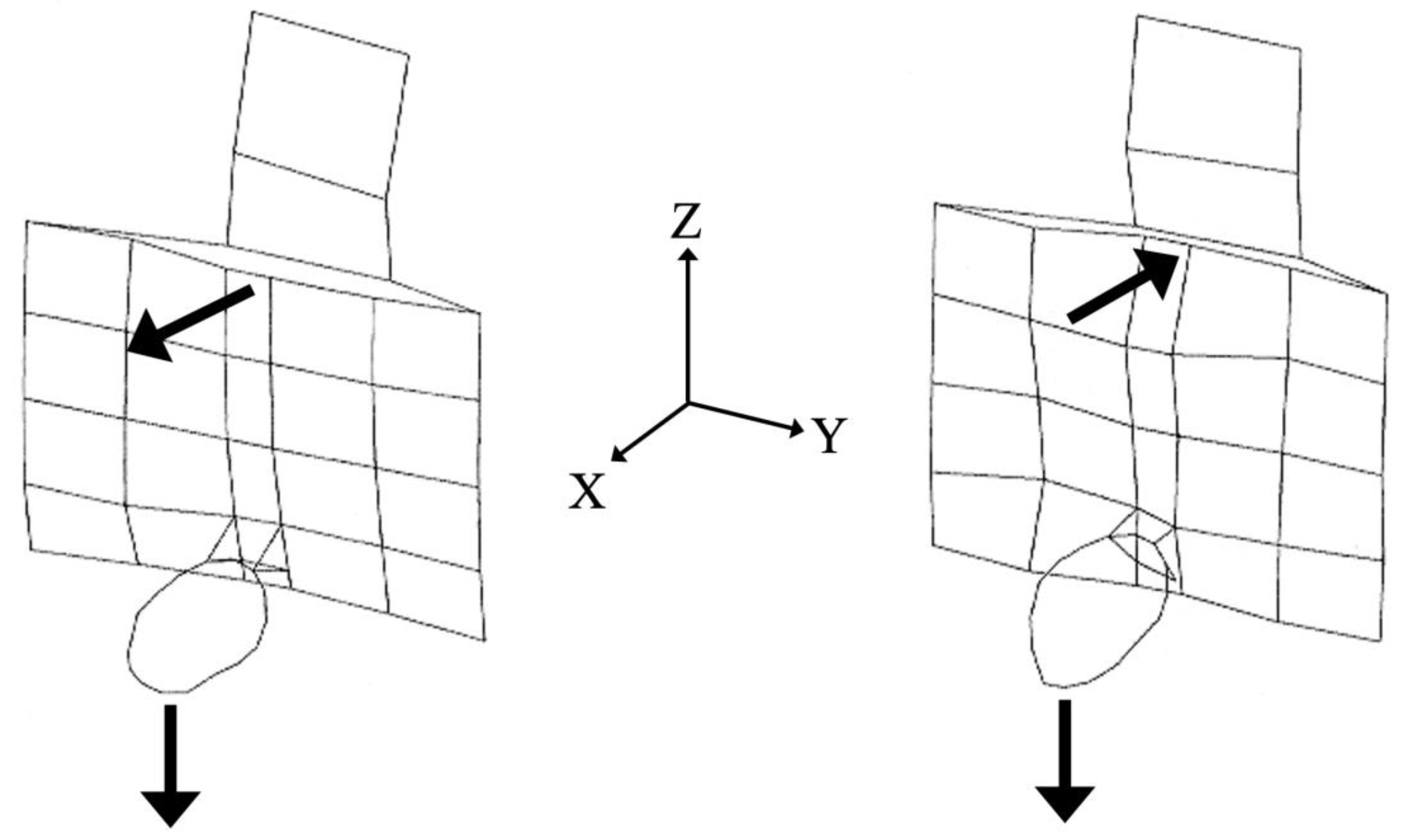
Figure 14.
Perturbation Mass Mp and Energy Rebound Testing Device, ERTD.
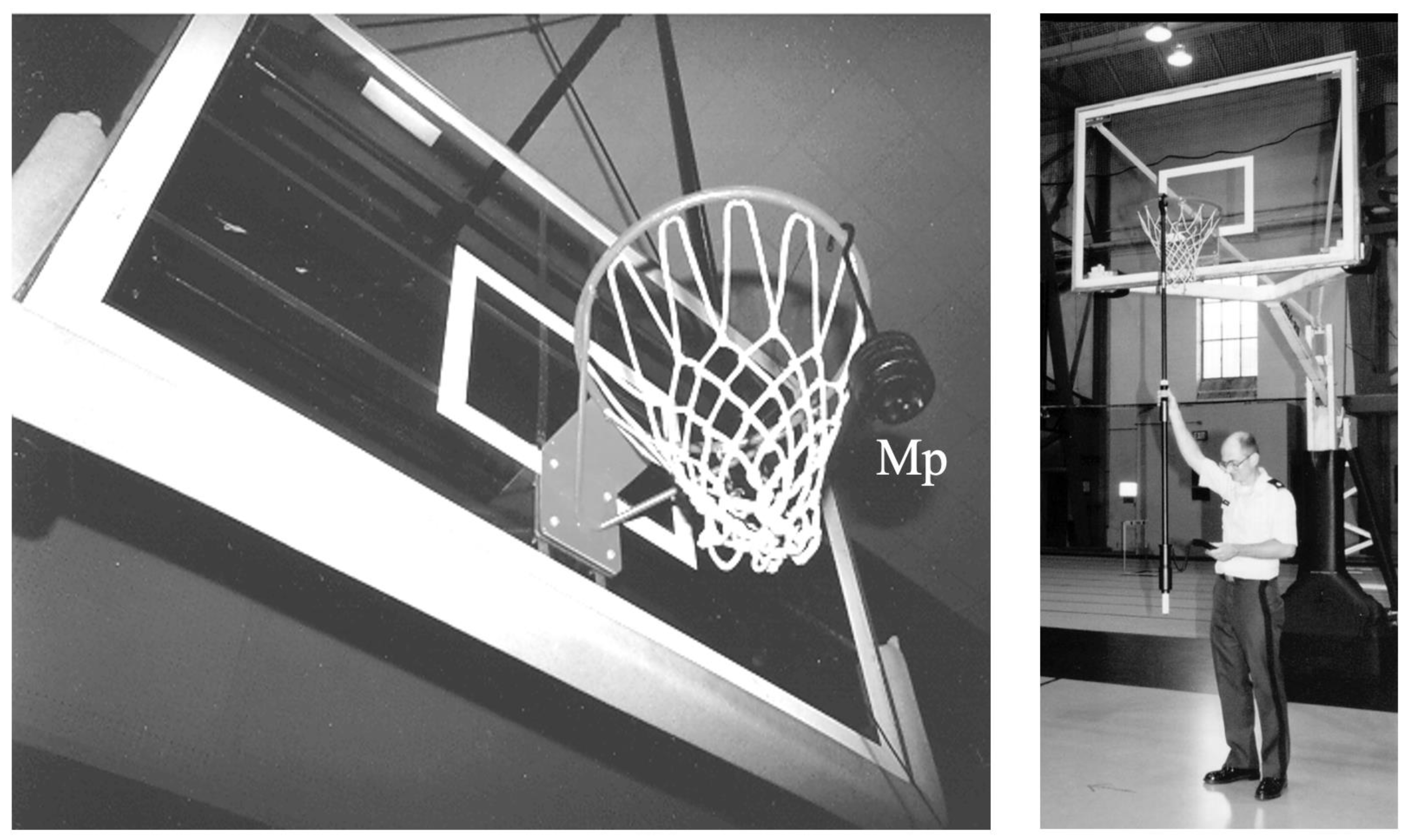
Figure 15.
Quadratic Equation for Eigenvalues λ as a function of Perturbation Mass Mp.
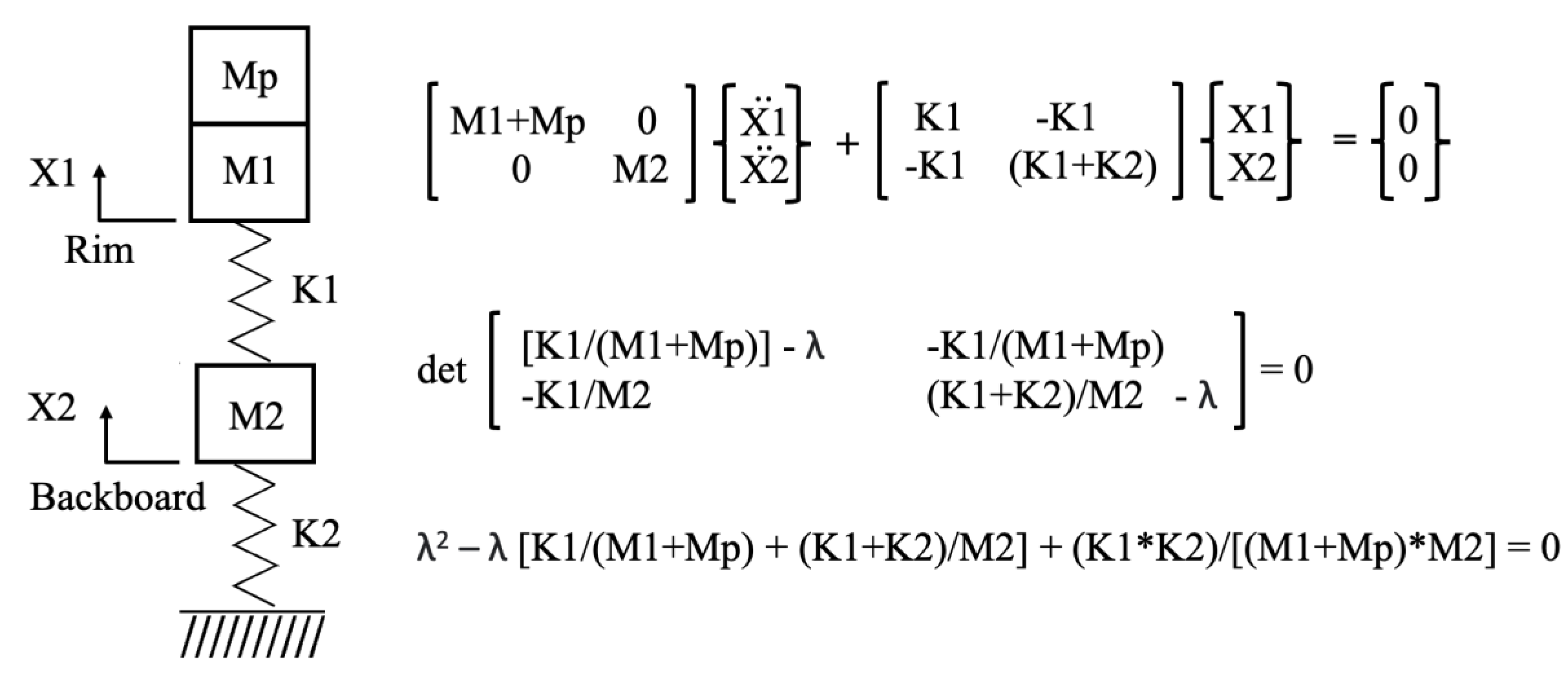
Figure 16.
ERTD reading in percent versus rim spring rate K1 in kN/m.
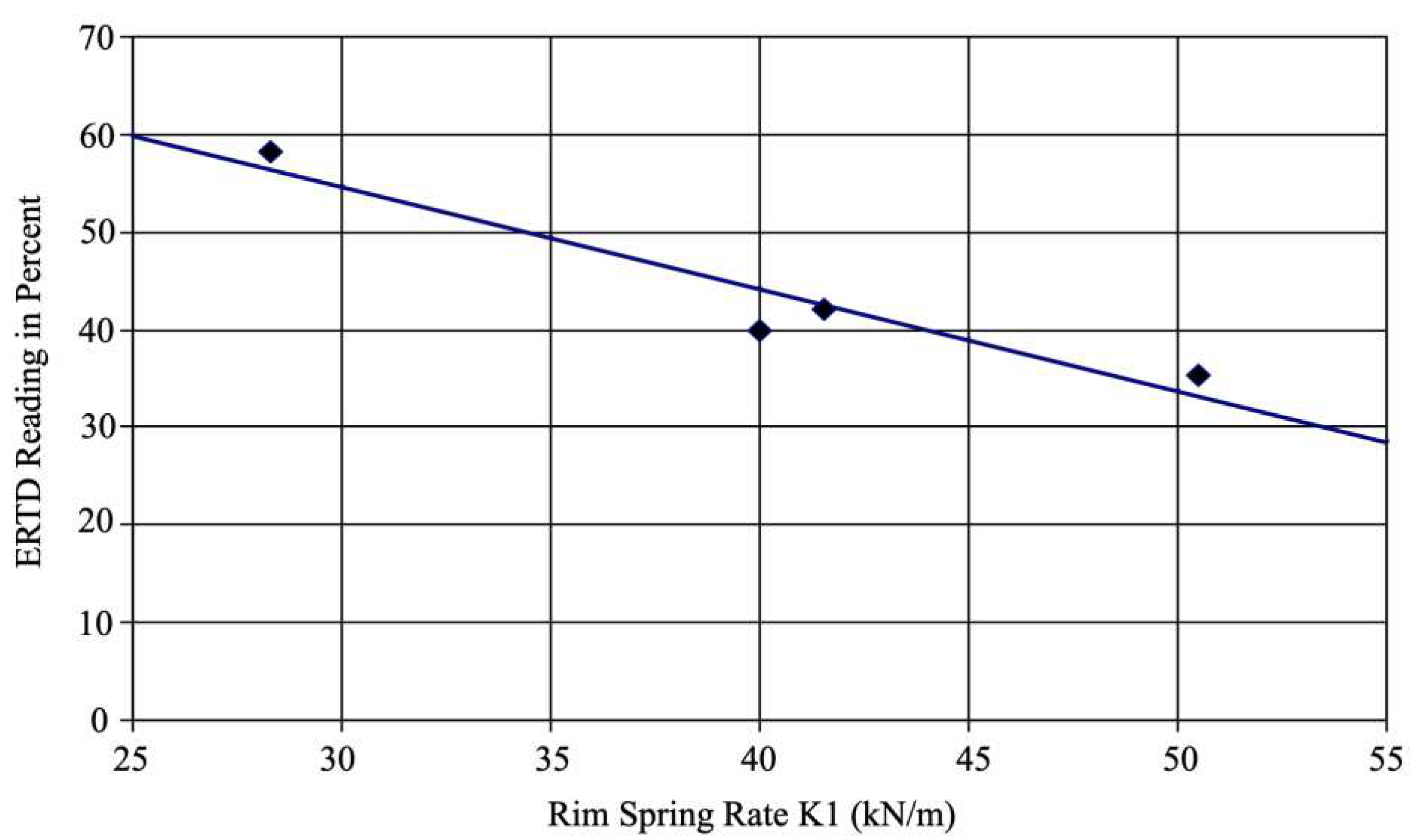

Table 1.
38 Nodes of Basketball Rim and Backboard: Cartesian Coordinates in millimeters.
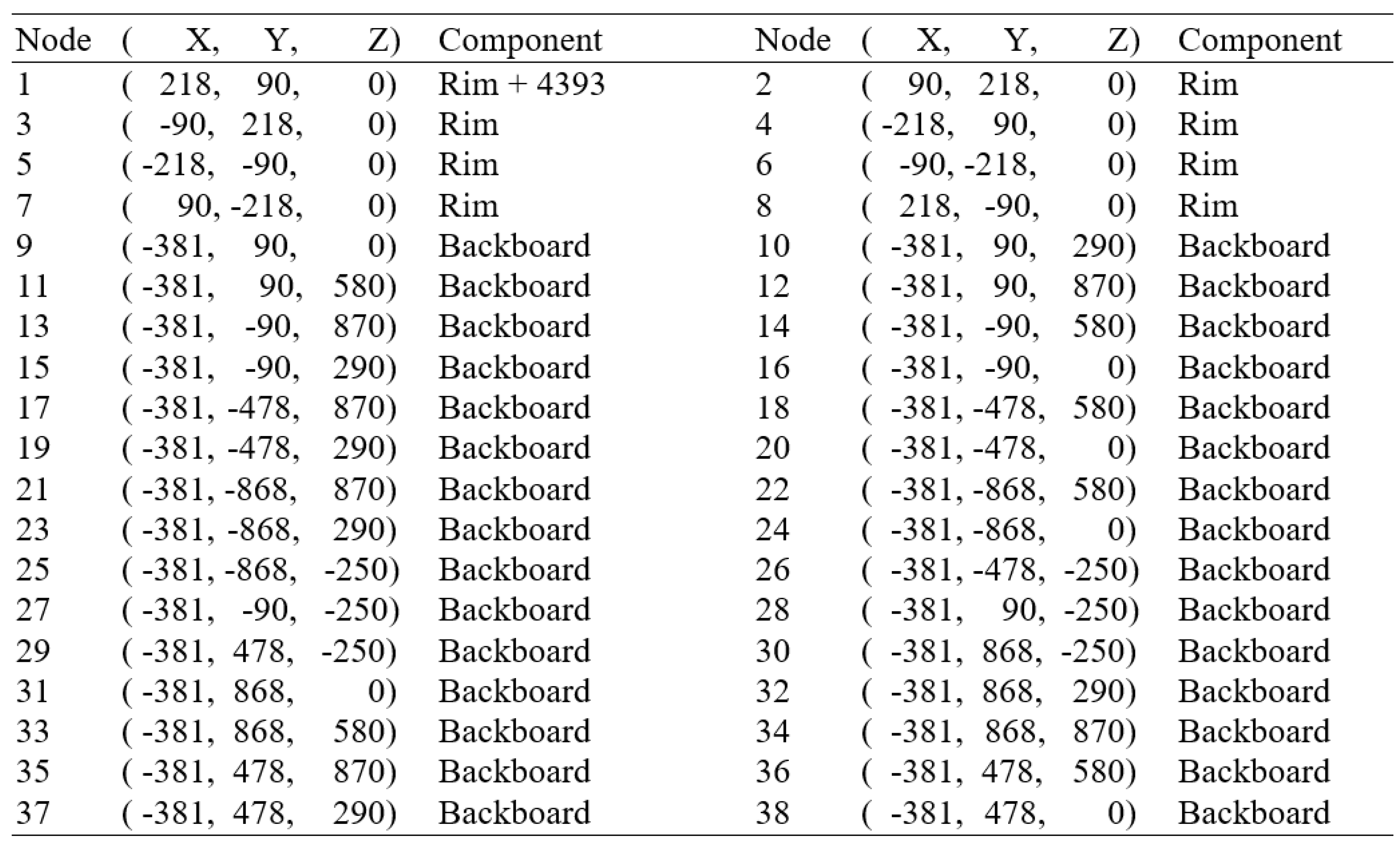
Table 2.
Display Sequence of 54 Lines Connecting 38 Nodes of Basketball Rim and Backboard.
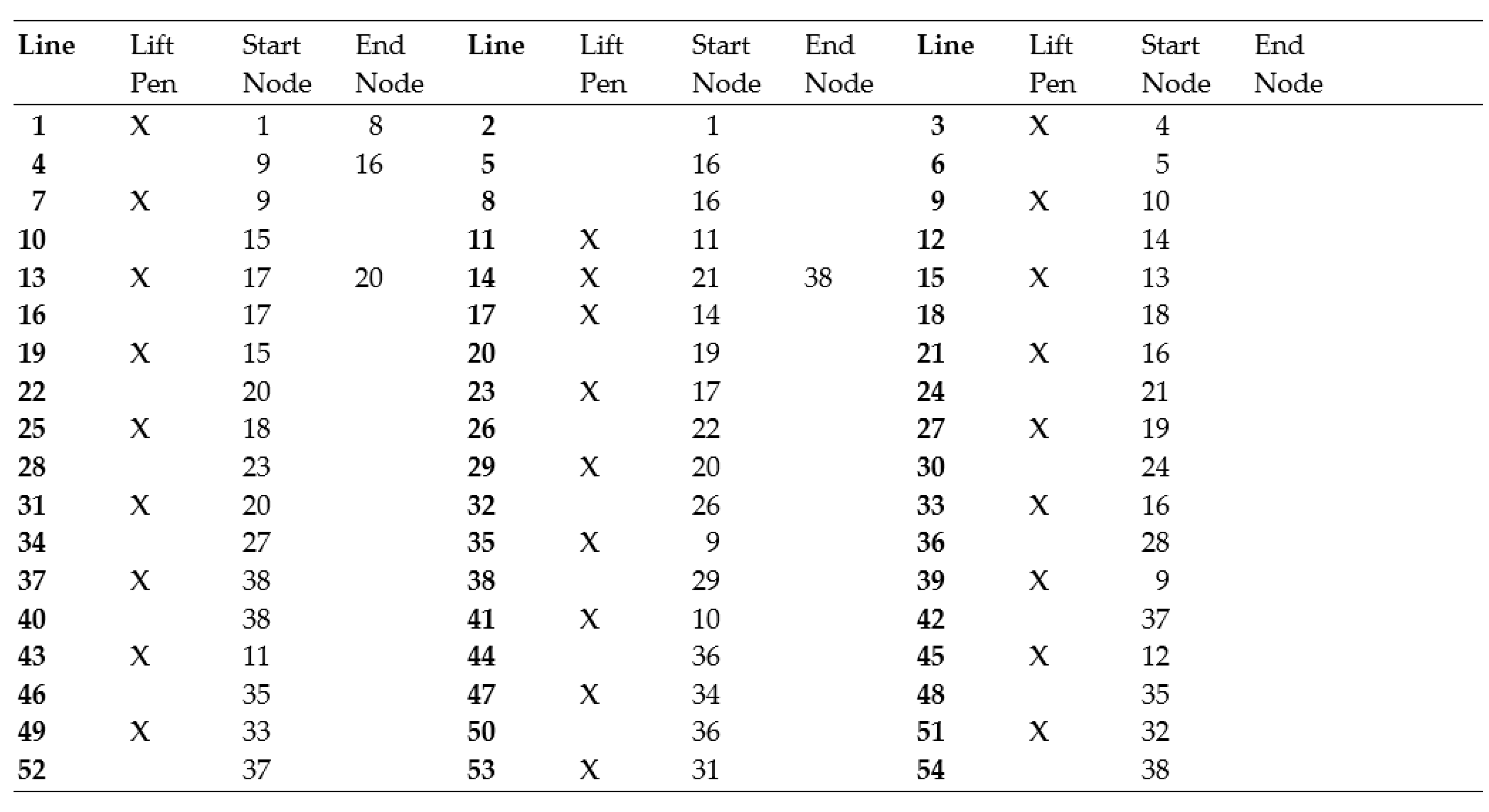
Table 3.
Frequency Ranges of Excitation for Various Impact Hammer Configurations.
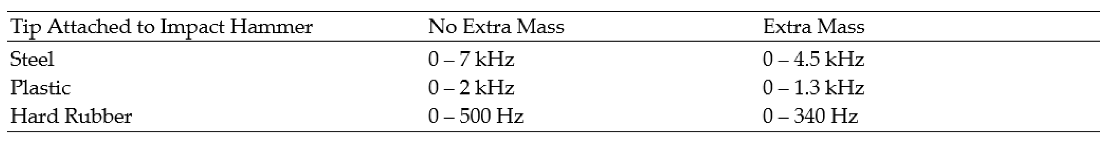
Table 4.
Windowing and Gains Assigned to 8202 Impact Hammer and 4393 Accelerometer.
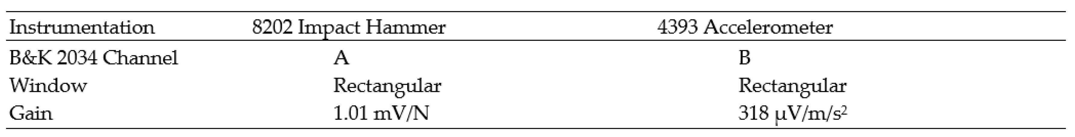
Table 5.
Six Peaks of Interest in Bode Plots with corresponding Left-Right Cursor Locations.
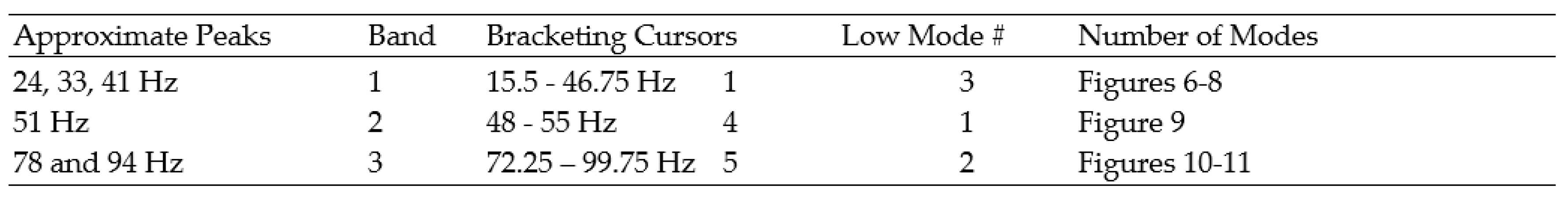
Table 6.
Tempered Glass in Hydra-Rib Backboards.

Table 7.
Summary of the Six Modes, their Frequencies and Damping Ratios ζ.
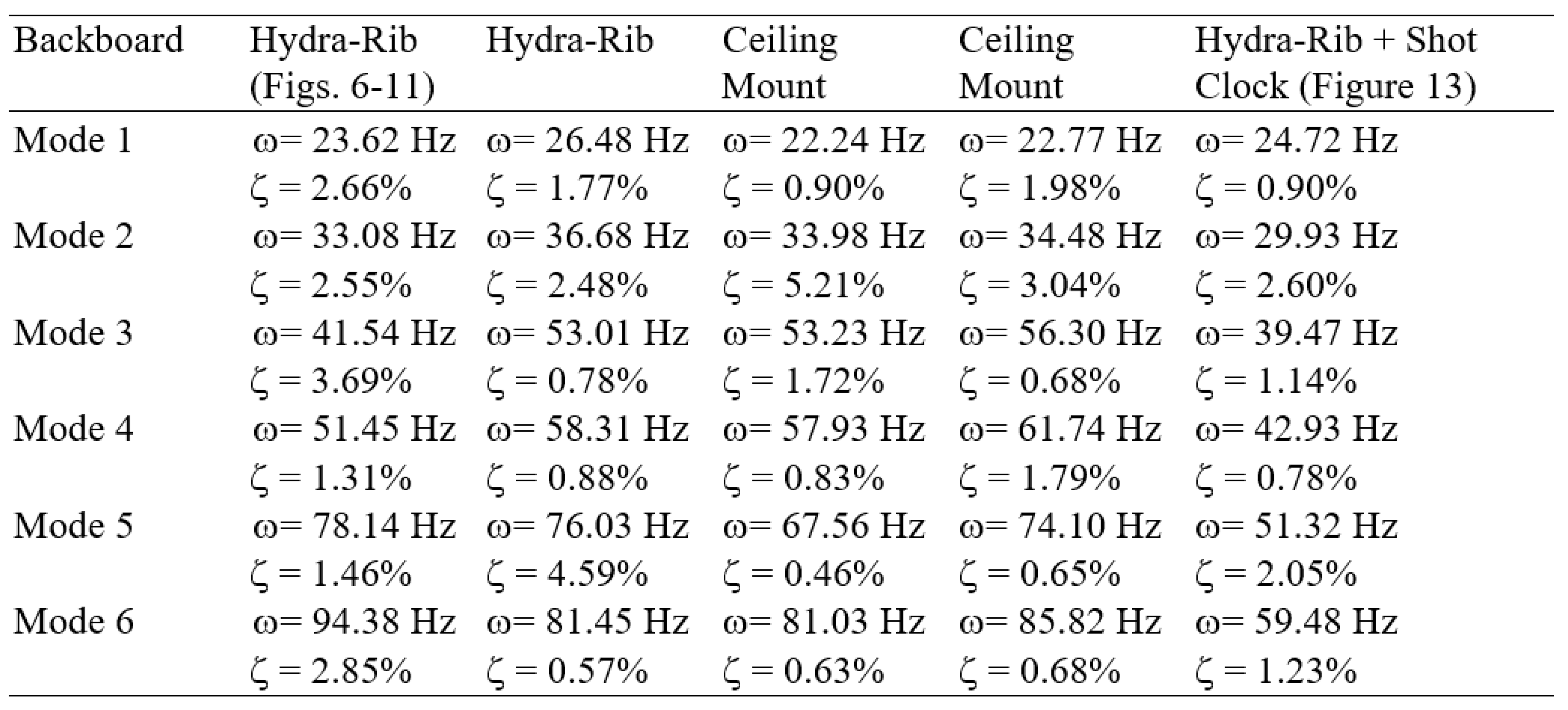
Table 8.
54 Nodes of Basketball Rim, Backboard, and Shot-Clock (in millimeters).
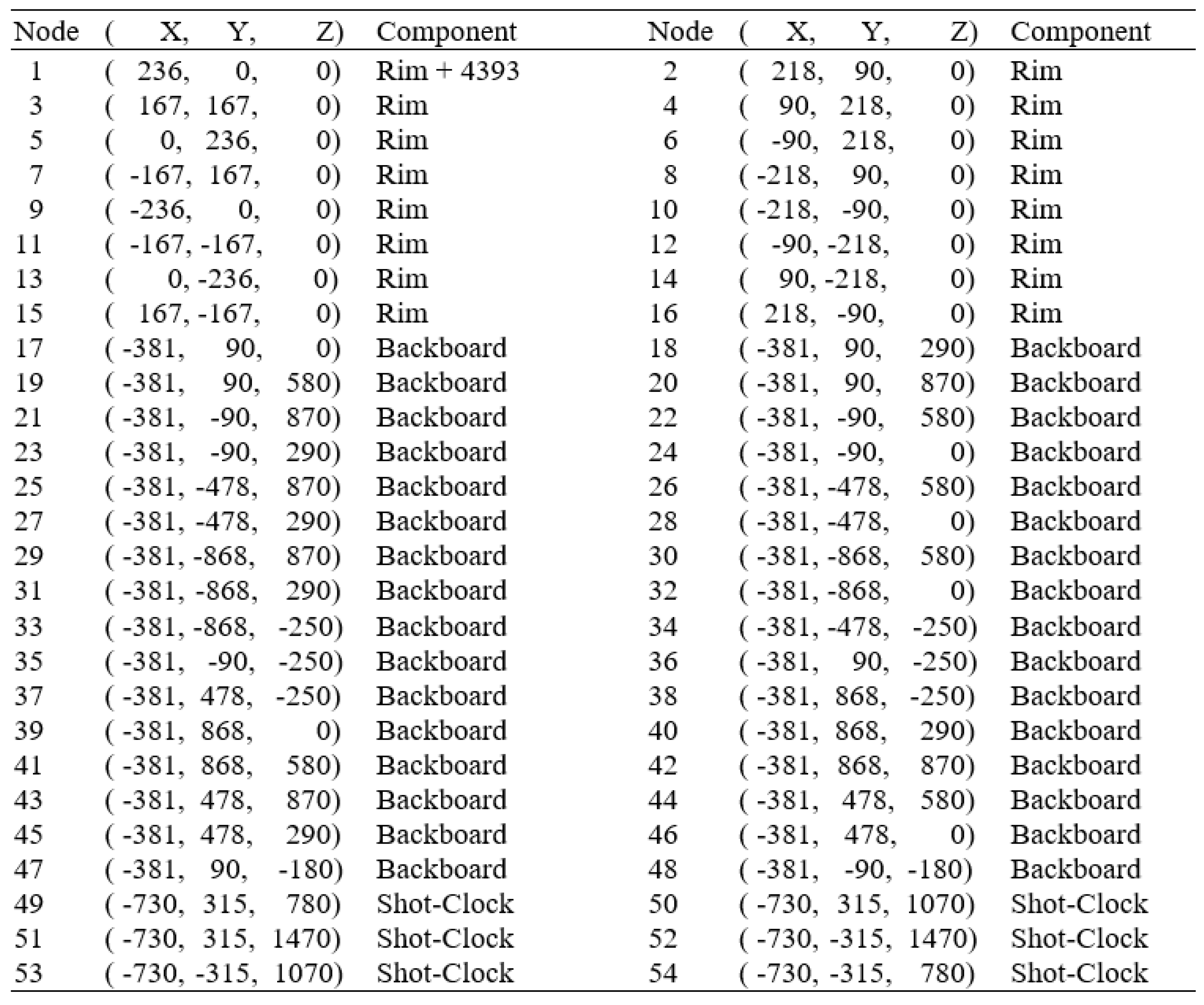
Table 9.
Display Sequence of 63 Lines Connecting 54 Nodes of Rim, Backboard, Shot-Clock.
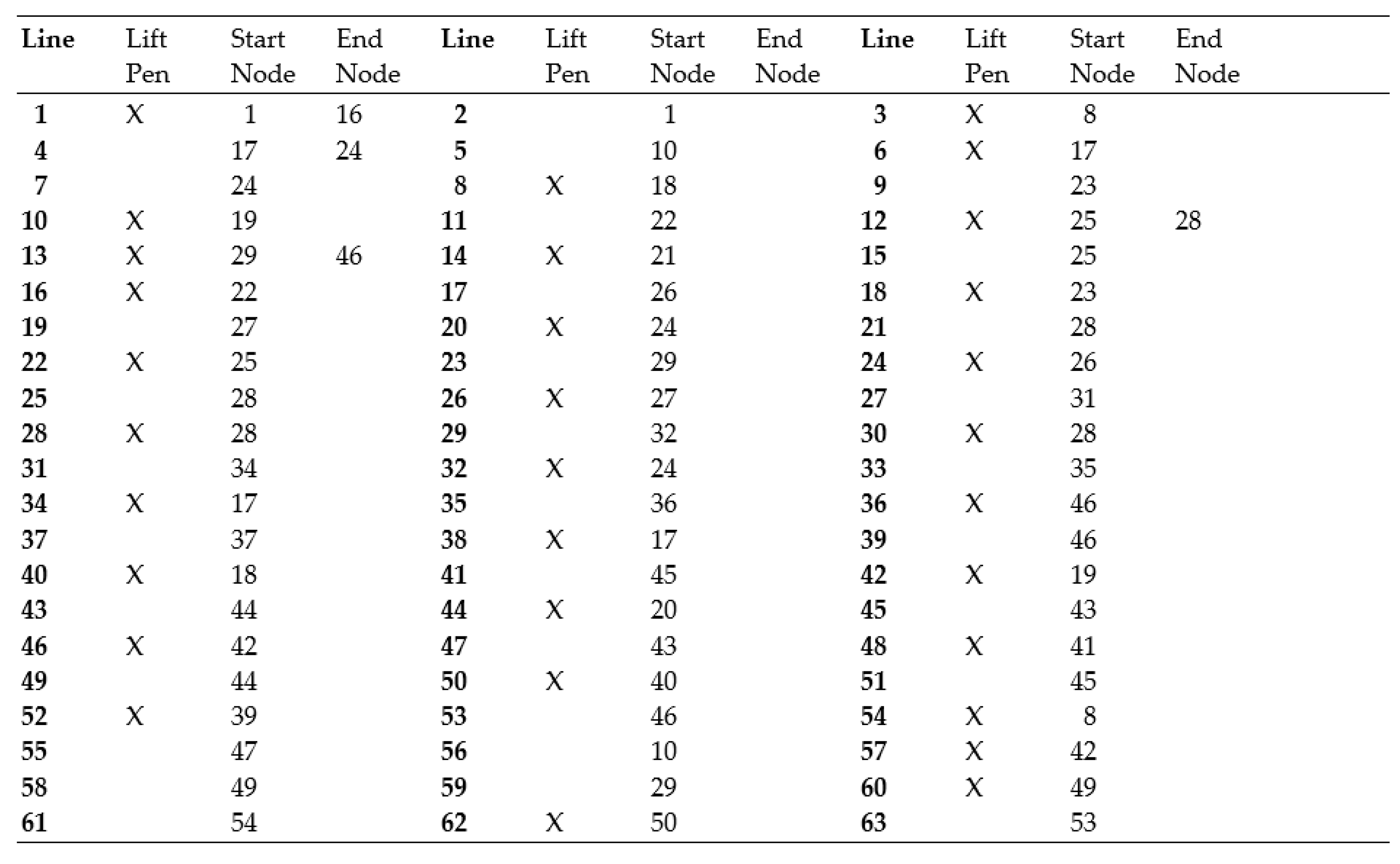
Table 10.
Calculation of Spring Rates and Masses of Rim and Backboard and ERTD Reading.
Disclaimer/Publisher’s Note: The statements, opinions and data contained in all publications are solely those of the individual author(s) and contributor(s) and not of MDPI and/or the editor(s). MDPI and/or the editor(s) disclaim responsibility for any injury to people or property resulting from any ideas, methods, instructions or products referred to in the content. |
© 2023 by the authors. Licensee MDPI, Basel, Switzerland. This article is an open access article distributed under the terms and conditions of the Creative Commons Attribution (CC BY) license (http://creativecommons.org/licenses/by/4.0/).
Copyright: This open access article is published under a Creative Commons CC BY 4.0 license, which permit the free download, distribution, and reuse, provided that the author and preprint are cited in any reuse.


