
Submitted:
07 August 2023
Posted:
08 August 2023
You are already at the latest version
Abstract
The accuracy of estimating changes in terrestrial water storage (TWS) using Gravity Recovery and Climate Experiment (GRACE) level-2 products is limited by the leakage effect resulting from post-processing and the weaker signal magnitude in adjacent areas. TWS anomaly in Dnieper River basin, where characteristic with medium scale and adjacent weak TWS anomaly, is estimate in this work. Two categories of leakage error repaired method (including forward modeling, Data-driven, single and multiple scaling factor) are employed. Root mean square error (RMSE) and Nash-Sutcliffe Efficiency (NSE) are used to evaluate the efficiency of methods. Compare to independent methods, TWS anomaly inverted by multiple scaling factor depending on CPC Soil Moisture model is more accurate in terms with RMSE 2.32 and NSE 0.88, which scaling factors corresponding to trend term 1.02, annual term 1.04, and semi-annual term 1.14. Further, comprehensive climate insights behind of the TWS anomaly were confirmed. The temperate continental climate of this River basin is shown, according to the variation of TWS anomaly in spatial domain. Snowmelt is significant role in TWS anomaly of Dnieper River basin, which is accord with the precipitation record and the 14 years temperature spatial distribution of February. Overall, we compare TWS anomaly recovered by single and multiple scaling method, the leakage signal originates mainly from semi-annual term of the TWS anomaly.
Keywords:
GRACE
; terrestrial water storage (TWS) anomaly
; leakage error recover
; Dnieper River basin
; climate pattern
1. Introduction
Terrestrial water storage (TWS), the summation of surface water, soil moisture, groundwater, ice, snow, and biosphere, is the critical component of the water cycle [1]. Reliable inversion of the TWS anomaly plays a key role in understanding the global or regional hydrological process and provides crucial information for water management. The research on regional hydrological TWS anomaly is limited by the in situ measurements of TWS. This is because current measurement methods and the characteristic of point-wise observation cannot obtain all of the TWS anomaly components. Along with rapid remote sensing development, particularly the implementation of the Gravity Recovery and Climate Experiment (GRACE) satellite mission, global or regional TWS research is possible. GRACE and its successor GRACE Follow on (GRACE-FO) have provided precise observations of the global temporal gravity field for the first time, which access to detect the TWS anomaly directly.
In practice, the monthly gravity fields, sets of spherical harmonics (SH) coefficients truncated at a certain degree, are used to infer regional TWS anomaly. However, the SH coefficients provided by GRACE RL-2 products should be filtered because of the inherent noise, including N-S “stripes” noise and short wavelength noise. The first filter, the Gaussian filter dedicated to solving short-wavelength noise, was devised by Wahr et al. [2]. It is an isotropic filter depending on the degree only. Some non-isotropic filters have been proposed in the literature. Based on the Gaussian filter, Han et al. have developed a filter that reconstructed the averaging radii as a function of order, in which the averaging process depends on the degree as well as order [3]. Swenson and Wahr designed a filter to remove the stripes noise so that the correlated errors are fit by a polynomial with an empirical moving window [4]. Following the ideal of Swenson and Wahr, Chambers and Chen modified it more concisely. They leave some portion of spherical harmonic coefficients unchanged, then fit the remnant even and odd coefficient pairs by the least squares and remove a polynomial of order 4 [5,6,7]. Duan et al. introduce two additional empirical parameters to the window width formula used by Swenson and Wahr [8]. This refined approach is based on the error pattern of the SH coefficients but also complicated the determination of unchanged portion and window width. Zhang et al. have devised another non-isotropic filter called the fan filter, which is a 2-D double filter including degree and order simultaneously [9]. There are many prior covariance-dependent filters as the variance-dependent filter and empirical orthogonal function filter [10,11], but we did not list them all.
The noise that existed in the SH coefficients was suppressed by amounts of filters that attenuated the signal as well. Besides, the regional average process for basin scale research also dampens the signal’s amplitude. The leakage error has generally been divided into two types. One type is the “leakage-in” error, caused by signals from adjacent areas leaking to interest one. The other type is the “leakage-out” error, which signals leakage is opposite to the “leakage-in” [12].
Many techniques or strategies have been proposed to repair signal attenuation and leakage errors. Generally, leakage error repair approaches are divided into two categories, that is the model-independent approach and the model-dependent approach. Hydrological or meteorological models are usually adopted for model-dependent approaches to calculate the scaling factor. Landerer and Swenson simulate the relationship between filtered and unfiltered global gravity fields by model GLDAS-NOAH and infer the scaling factor [13]. Pokhrel et al. employ the GRACE results repaired by the scaling factor approach and assess the role of groundwater in the Amazon water cycle [14]. The hydrological model PCR-GLOBWB is used to generate the scaling factor for recovering the TWS anomaly of the Yangtze River basin [15]. As convenient, it has been widely applicated in global or regional TWS anomaly research. At the same time, it is dependent on certain hydrological models possessing discrepant performance in different regions.
The other leakage error repair approach category is model-independent without auxiliary model data. Baur and Sneeuw conducted a methodology of point-mass modeling to evaluate Greenland ice mass loss to avoid leakage effects arising from the filter process [16]. Chen et al. have analyzed the mechanism of leakage error from the SH truncation and spatial filtering detail and devised a method of constrained forward modeling to counteract that error [17]. Mu et al. proposed an approach of Tikhonov regularization with the L-curve method to reduce the leakage effect based on the correction equation established by Tang [18]. They successfully estimated the mass change rate in Greenland and Antarctica [19]. Vishwakarma et al. confirmed that signal leakage not only affect the amplitude but also the phase exhibited in the time domain and proposed a strategy to approach attenuation and phase shift called the Data-driven method [20,21].
Though lots of approaches have been proposed for precise inversion of TWS anomaly on a regional scale. However, most research concentrated on regions or river basins like Amazon, Greenland, Indus, Antarctica, Yangtze River, Tibetan Plateau, Congo, Nile, and so on [22,23,24,25,26,27,28]. Those regions are characteristic of larger areas (>106 km2) or stronger signals attributed to mass changes. Even though some literature focuses on the medium and small basins [29], such as Finland, the Liao River basin, and the Aral Sea basin [30,31,32,33], distinctly mass changes or redistributions also demonstrate in those regions. However, rarely focus have been switched to the regions with medium scale and weak adjacent areas.
The climatic conditions in the Dnieper River basin are complex, for the spatial heterogeneity of precipitation from northwest to southeast impact of temperate continental climate [34]. The complex climate feature will be captured by inversed TWS anomaly from GRACE temporal gravity field. The main aim of this study is to obtain the accurate TWS anomaly in the Dnieper River basin using GRACE data. To that end, two categories of leakage error repair approaches were tested. Furthermore, we have revealed the comprehensive climate significance behind the TWS anomaly in terms of spatial and time domains by the inversed GRACE results combined with hydrological and meteorological data.
2. Materials
2.1. Study Area
The Dnieper River Basin, shown in Figure 1, is one of the largest rivers in Europe and covers an area of 511 thousand km2 [35]. The River basin spans three countries, Russia, the Republic of Belarus, and Ukraine, and includes many sub-streams [36]. The Dnieper River is perennial originally from the south of the Valdai Hills in Russia and flows through Russia, Belarus, and Ukraine, and finally empties into the Black Sea 30 kilometers southwest of Kherson [34]. The Dnieper River has four main tributaries, and six reservoirs are built along the river [37].
Conventionally, with Kyiv and Zaporizhzhia as the boundary, the Dnieper River has been decomposed into three parts (upstream, midstream, and downstream). For the upstream, it is mainly located in a forest area with Peat-podzolic soil. Besides, this area has a well-developed river network, accounting for four-fifths of the annual flow of the whole basin, with the most significant and longest tributaries, i.e., the Berezina River. The midstream and downstream it is mainly covered by steppes with black soil. however, most of those regions had been reclaimed for agriculture.
The climate of the Dnieper River basin is warm and humid. From northwest to southeast, the continental climate is gradually prominent. The precipitation in this basin exhibits the properties of decreasing from north to south. Turning to the adjacent areas of the Dnieper River basin, the Black Sea is the distinctive region dominated by the Mediterranean climate. TWS anomaly of the Black Sea from GRACE is vulnerable to contamination from land hydrology due to the relatively weak fluctuation of mass change contrasted to adjacent land areas. Besides, the Dnieper River basin is the main region supplying the crops for Europe, even globally. Considering the factors of climate and agriculture, the performance of the TWS anomaly estimated from GRACE for the Dnieper River basin is imperative.
2.2. Datasets
In this work, GRACE Level2 (Release 06) monthly gravity data sets combined with other climate and hydrological data sets are used for extracting information about mass changes. Details of the data sets can be found in Table 1.
2.2.1. GRACE Data
GRACE solutions are expressed by spherical harmonic coefficients up to degrees 60 or 96. The relation between spatial resolution and spherical harmonic coefficients can be approximately 20000km/L. so the GRACE RL-06 results can attend a theoretical maximal spatial scale of 330km or 220km. The newly released RL-06 models mainly come from three scientific centers: the Center for Space Research (CSR), Geo-Forschungs-Zentrum (GFZ) Potsdam, and Jet Propulsion Laboratory (JPL). All data sets can be obtained from the website in Table 1. In this study, we adopt the RL-06 products with a maximal degree of 96 from CSR—the study period from January 2003 to December 2016 has 151 monthly solutions. As the influences of gravity satellite operations, 17 months of solutions are missing in the study period.
Following the general procedure, the C20 coefficient is replaced by independent measurement from satellite laser ranging (Technical Note TN-11) [38]. The degree 1 coefficients have been replaced by estimations using the method of Sun et al. (Technical Note TN-13) [39]. Next, the glacial isostatic adjustment (GIA) effect is removed with the method suggested by Geru A et al. due to the Dnieper River basin being located in an area influenced by the last glacial period [40].
2.2.2. Snow Water Equivalent and Soil Moisture from GLDAS and CPC
Snow water equivalent (SWE) and soil moisture (SM) derived from the GLDAS are adopted for analyzing the TWS change in the Dnieper River basin [41]. Global Land and Data Assimilation System (GLDAS) was developed jointly by the National Aeronautics and Space Administration (NASA) Goddard Earth Science Data Information and Services Center (GES DISC) and National Oceanic and Atmospheric Administration (NOAA) National Center for Environmental Prediction (NCEP) [42]. Up to now, GLDAS drives four land surface models (LSMs): Noah, Catchment (CLSM), the Community Land Model (CLM), and the Variable Infiltration Capacity (VIC). The datasets are organized as the spatial 1°×1° or 0.25°×0.25° resolution and 3-hourly, daily, and monthly temporal resolution separately [43,44]. In this article, we select the Noah datasets of version 2.1 from 2003 to 2016 with monthly time resolution and 1°×1° spatial resolution. The variates, including SM at a depth of 0 to 200 cm, SWE are used to simulate the TWS in the Dnieper River basin.
The CPC (Climate Prediction Center) Soil Moisture V2 data are used to simulate the TWS for validation. The CPC soil moisture data sets provide the monthly and daily global soil moisture data at the resolution of 0.5° from 1948 to the present [45,46]. The data sets are obtained by a land model, with the driving input fields including CPC monthly precipitation overland and global temperature from global reanalysis [47].
2.2.3. Total Water Storage form WGHM
The priori total water storage (TWS) information is needed as input when using the scaling method to restore the GRACE leakage effect described in 2.3.3. Here WaterGAP Global Hydrology Model standard version (WGHM 2.2d), a sub-model of the model of WaterGAP 2, is used to extract TWS anomalies. Excluding water in the glaciers, WGHM encompasses soil, snow, and canopy components in the vertical direction and lakes, man-made reservoirs, wetlands, groundwater, and rivers in the lateral direction. The WGHM 2.2d has a time from 1901 to 2016, 0.5° spatial resolution, and monthly temporal resolution. The WGHM data is extracted and resampled as 1° by 1° grid data from 2003 to 2016 to compare with GRACE results [48].
2.2.4. Precipitation from GPCC
Usually, the TWS anomaly detected by GRACE is closely related to precipitation at the river basin. For analysis and verification, the precipitation of the Dnieper River basin from GPCC products is introduced. The precipitation data from the Global Precipitation Climatology Center (GPCC) are constructed based on 124000 in situ measuring stations distributed worldwide [49]. All GPCC products are available in the spatial resolutions of 1°, 0.5°, 0.25° and 2.5° latitude and longitude, and the temporal resolution of month [50]. In the paper, we adopt the data sets from 2003-2016 in 1° spatial resolution.
3. Methods
3.1. GRACE Data Processing
Generally, the gravity field of the Earth is expressed by the relation of between geoid S and SH coefficients as in eq.1,
Where and are colatitude and longitude, is the average radius of the Earth, is normalized associated Legendre functions, and and are the SH coefficients which have provided by GRACE RL-06 products.
The gravity changes could be inferred using the multiple monthly GRACE RL-06 harmonic coefficients. In other words, the mass transition with time within the Earth or above its surface is extracted. The harmonic coefficients from GSM files have already removed the effect of the atmosphere, tides, and ocean. The remaining sources of time-variable mass changes are treated as a thin layer at the earth’s surface. Therefore, one can approximate the vertically integrated mass as a surface mass density [2]. Equation 2, given by John Wahr, is adopted,
Where is the average density of the Earth, are the load love numbers obtained from Han and Wahr [51], and / are the variation of the coefficients. In practice, we convert to equivalent water height (EWH) by:
A two steps filter strategy has been implemented in this paper, as the original GRACE signal includes the noise of high frequency and correlation. The south-north noise in the different odd and even high-degree coefficients for the same order has been first confirmed by Swenson and Wahr [4]. To suppress it, a method devised by Chen et al. in 2009 has been used [52]. The basic idea of this means is supposing the fitted results as the correlation error. For the coefficients 6 and above it, a polynomial of fourth order is constructed and fitted by the least square method. Then the polynomial results are removed from corresponding spherical harmonic coefficients derived from GRACE observation. Next, to reduce the high-frequency noise, a Gaussian filter with a halfwave length of 300 km is carried out following as eq.4,
Where are smoothing factor of Gaussian associated with degrees of harmonic coefficients.
A regional average kernel function is used to extract the Dnieper River basin mass change,
Generally, is expanded as an SH function. According to the orthogonality of harmonic function, coefficients of , ,and , will be calculated and then be employed for extracting the basin mass change combining with eq. 6,
Where is the regional anomaly of EWH, all other symbols in eq. 6 are the same as aforesaid. But from the view of signal processing, the average kernel function is equal to a rectangular filter in the spectral domain, leading to signal leakage. The weighting function method widely used in the digital signal processing domain is adopted to reduce the leakage caused by the sidelobe effect in the filter. Here the weighting function is defined as a cosine function of latitude, and then the local mass changes can obtain by the eq. 7,
However, the signal has been damped due to spherical harmonic truncation and Gaussian spatial smoothing. In this article, the forward modeling (FM) method, Data-driven method, and scaling method are used to restore the GRACE observed signal.
3.2. Forward Modelling Approach
The FM approach is a procedure of iteration, and a brief instruction is represented as follows:
- (1)
- we regard the GRACE observations as the initial mass anomalies in the Dnieper basin. That means the mass variation within the Dnieper River basin is defined as GRACE observations, and beyond the areas are considered zero.
- (2)
- the initial mass anomalies are expanded to the SH coefficients at the degrees and orders 96. In addition, a 300 km Gaussian filter is applied same as GRACE L2 data sets done. Then the forward model mass anomaly is obtained.
- (3)
- the residual between the initial mass anomaly and the forward modeling mass anomaly is added to the initial mass anomaly. In previous studies, a scale factor of 1.2 is recommended, which can accelerate the convergence of the iteration, that is, . Here, we choose 0.6 as the scale factor according to the data experiment. The new initial mass is repeated for the second step until the difference is less than a certain threshold or after a certain number of iterations. In this research, we set the number of iterations is 50.
3.3. Scaling Approach
The scaling factor is critical for the scaling approach to recover the damped GRACE observation and depends on the prior hydrological model. The mass variation derived from hydrological models is considered the true mass variation in the river basin. The hydrological model is expanded in SH coefficients, truncated at degrees and orders 96, and smoothed by a 300 km Gaussian filter. The difference between the original hydrological model and the filtered is attributed to the leakage effect.
A single scaling factor for the Dnieper River basin is obtained by fitting the unfiltered model time series and filtered time series with the least square method, that is:
Where k is the scaling factor. Three single scaling factors are subsequently obtained by filtering the hydrological model GLDAS, CPC, and WGHM at the river basin scale.
Generally, TWS variation expressed by time series includes the terms of long trend and seasonal period as depicted in Figure 3. A reasonable approach is that the time series of unfiltered and filtered models GLDAS, CPC, and WGHM are decomposed into long trend term, seasonal and residual components as eq. 9,
For this purpose, a least squares model is used for fitting the time series as eq. 10.
Where is the TWS anomaly averaging over the Dnieper River basin at the month, A represents the TWS anomaly for the mean times, B is the long trend linear terms, k is the numbers of period, is the period, and are the amplitudes of the cosine and sine terms of the same period , and is residuals. Nevertheless, the periods could not be determined directly from the time series of hydrological models.
3.4. Data-driven Approach
In the time domain analysis, Vishwakarma has shown that the filtering process not only weakens the amplitude of the time series but also changes the phase [21]. There are two forms of Data-driven approaches. One is the scaled form which can be described as equation (11):
Where is the corrected time series, is the time series obtained from filtered GRACE spherical harmonic coefficients models, is leakages obtained by toe times phase shift, and s is the scale factor.
For equation (11), is obtained by the method described in sec 3.1. the scale factor s is calculated by the equation (12). We skip over the process of derivation and give the equation as,
Where denotes the surface of the earth, is the kernel function same as equation (5), is the filtered kernel function. The scale factor s is independent of any other hydrological models.
For the leakages calculation, we need to filter the GRACE field twice. The leakage time series and are calculated by equations (31) and (32) represented in Vishwakarma’s paper [20]. Then we shift the to with the phase difference and calculate the mean ratio between them. Finally, we shift the with the phase difference and multiply the mean ratio.
Another type of Data-driven approach is called deviation Data-driven. Unlike the scale Data-driven approach, the modified approach introduced the deviation item instead of the scale factor. We give the method directly as,
Where is determined by . more details about the scale and deviation Data-driven approach can be found in Vishwakarma [21].
3.5. Uncertainty Estimates and Validation Method
For evaluating the relative efficiency of different approaches, several assessment indexes are applied to quantitatively analyze the uncertainty of estimates of TWS anomaly that are restored by FM, Data-driven, and scaling approaches. The root mean square error (RMSE) is taken to assess the uncertainty of the restored GRACE-derived TWS anomaly, which is described as follows,
Where is the corrected time series deriving from GRACE, is the time series of true mass variation in a river basin, and n is the number of months in the study period. In practice, we propose to use the MASCON products released by CSR as the true mass variation. An RMSE close to zero indicates excellent agreement between the restored and true values.
Similar to the RMSE method, Nash-Sutcliffe Efficiency (NSE) is often used to evaluate the performance of approaches.
Where is the mean of the true value, and other symbols are the same as above. An NSE value close to 1 means great performance for the corrected results.
3.6. Cross Wavelet Transform
Especially, a time-frequency method is introduced to validate the components of seasonal variation from the results simulated by hydrological models, that is, cross wavelet transform (XWT). XWT is devised by A. Grinsted et al. first, and the basic idea is to examine two-time series together in the time-frequency domain to extract the features of trend or periodicities [53]. The XWT was applied to the time series of GRACE observation and the one simulated from hydrological models. Then, one could examine whether a region with large common power and a consistent phase relationship exists. This region may illustrate and validate the climate variability derived from GRACE. XWT is constructed by two continual wavelet transforms given the CWT results of two time series derived from GRACE and hydrological models.
4. Results and Discussion
As mentioned in Section 2, four approaches are used to reduce the leakage error combined with three hydrological models. We show the corrected results as two groups according to the model properties. One is the auxiliary model-independent approach, including the FM and Data-driven approaches, and another is dependent types containing the single and multiple factor approaches.
4.1. Results of Model Independent Approach
We represent the TWS change in Figure 2, Figure 3 and Figure 4 and the performance in Table 2, which is inversed by the model-independent approaches, including the FM and Data-driven approaches.
4.1.1. Convergency of Forward Modeling Approach
Figure 2 shows the trend of TWS anomaly recovered by the FM approach described in Section 3.2 in the spatial domain. Comparing the a) and b) in Figure 2, the mass changes rate is recovered from -12±-1.44 mm/a to -14.1±-1.7 mm/a after recovery by FM approach. After the filter process that is the same as GRACE, the recovered mass rate c) is -10.7±-1.28 mm/a, close to the initial mass rate a). Though a) and c) have the characteristic of boundaries both at the values of -5 mm/a and -10 mm/a, those forms of expression vary. For Figure a), the mass rate varies in a fan region formed by the boundary, while for Figure c), the mass rate varies in ring regions formed by the boundaries. In Figure c), boundaries tend to converge. In other words, the leakage error effect is converged behind the FM approach’s correction. The residuals between the initial mass rate and the filtered mass rate are depicted in d) of Figure 2 to analyze the effect of the FM approach. As d) shows, most of the region in the Dnieper River basin mass rates close to zero. But there are two regions with residuals of about 4 mm/a and -5 mm/a in the northwest and southeast of the Dnieper River basin. Those residual anomalies may not be neglected, considering the range of water height variation. This discrepancy may appear apparently in the time domain.
Figure 3 shows the time series of the TWS anomaly corrected by the FM approach in the Dnieper River basin from 2003 to 2016. In contrast to the time series derived from CSR Mascon products, the corrected time series have a fine consistency. All the results represent the same variation trend. The TWS anomaly exhibits a rising trend from 2003 to 2006 and represents a declining trend for the rest of the research period. If we examine the efficiency of the FM approach for two parts at the demarcation point of 2006, the deficiency of the FM method may be revealed. From 2003 to 2006, the difference between the corrected and Mascon time series was magnified. In other words, the FM method increases the trend of separation between filtered time series and ‘true’ time series. After 2006, the corrected time series is more closed to the ‘true’ time series. The FM method property may cause the reason for this phenomenon, that it is more sensitive to the trend of time series. That is to say, at the increasing period, the FM method magnifies the increasing trend, and vice versa.
4.1.2. Phase Shift Error Caused by Data-driven Method
Besides the FM method, two Data-driven approaches have been conducted for the same river basin. Figure 4 shows the results recovered by two forms of Data-driven approach in the time domain. A first observation is that all corrected time series are well agreed with the ‘true’ time series. Both recovered time series show a trend closer to the ‘true’ time series than the filtered results. Two forms of Data-driven approaches have reduced the deviation caused by the filtering process, but the scale Data-driven approach is less efficient than the deviation form. Nevertheless, both forms have relatively abnormal peaks in the spring of 2005, 2011, and 2015. The reason for this may be the influence of the Data-driven approach. For the processing procedure of the Data-driven approach, a critical step is the phase difference calculation for the filtered time series. Examining the filtered time series, the characteristic of bimodal distribution is manifested in the spring of 2005, 2011, and 2015. When calculating the phase difference of the filtered time series, the bimodal distribution could be distorted by the results as a phase shift. For instance, the peak of the time series corrected by the scale Data-driven approach in the spring of 2005 shift near two months ahead of the ‘true’ one.
4.1.3. Comparison of Model Independent Approaches
The uncertainty estimates of two kinds of independent approaches by the means are described in Section 3.5 and shown in Table 2. The deviation Data-driven approach performs best with 2.7 RMSE and 0.84 NSE, respectively. The rest of the independent approaches are almost equal capability to weaken the effects of leakage. Particularly, we will give more words about the scale Data-driven approach. From Table 2, the results repaired by the scale Data-driven approach are the worst in terms of RMSE and NSE. Compared with the deviation Data-driven approach, the magnifying process calculated by multiplying the scaling factor k magnified the attenuated amplitude and residual errors simultaneously. It is important to note that the scaling factor k in the scale Data-driven method only depends on the regional kernel function. That is to say, the scale Data-driven approach is independent of any auxiliary hydrological or meteorological models. Based on the above analysis, the deviation Data-driven approach is more accurate for repairing damaged signals caused by filtering in the three model-independent approaches.
4.2. Results of Model Dependent Method.
Like Section 4.1, the TWS anomalies inversed by single and multiple scaling factor approaches are shown in Figure 5, Figure 6, Figure 7 and Figure 8.
4.2.1. Inefficiency for Multiple Trends by Single Scaling Factor Approach
Corresponding to model-independent approaches, two model-dependent approaches are implemented in this article that is single and multiple scaling factor approaches. Following the method described in Section 3.3, the restrained signal derived from GRACE products is restored and depicted in Figure 5, Figure 6, Figure 7 and Figure 8.
In Figure 5, The recovered trend of TWS anomaly by the single factors calculated from three hydrological models holds a similar variation pattern. The TWS anomaly is decreasing from northwest to southeast, which agrees with the feature of the climate of the Dnieper River basin. There is almost no distinction between filtered results (a) and corrected results (b) and (c). Those trends follow the scaling factors 1.073 and 1.072 calculated from the hydrological model WGHM and GLDAS. It is implied that both WGHM and GLDAS are less sensitive to the Dnieper River basin. Compared with Figure (a), the trend of TWS anomaly in Figure (d) has been enhanced visibly. The TWS change rate has been recovered from -12±-1.44 mm/a to -13±-1.56 mm/a with the single factor 1.082 derived from the CPC soil moisture model. Despite the consequence of (d) in Figure 5 possessing an obvious variation, there is no evidence to confirm that it is relatively more effective in leakage error repairing. Further analysis of the efficiency of the single factor approach will be conducted in the time domain.
In Figure 6, the TWS anomalies corrected by the single factor approach, derived from the hydrological model GLDAS and WGHM, are barely seen. This situation is in agreement with the trend depicted in the spatial domain. Like the FM method, the time series in Figure 6 are divided into two parts in 2006. From 2003 to 2006, all corrected time series are away from the ‘true’ time series relative to the filtered one. From 2007 to 2016, the corrected time series are close to the ‘true’ time series. This phenomenon existed in both Figure 5 and 6, implying that the corrected trend term dominates the results recovered by the single factor approach. All the results mentioned above depicted in both spatial and time domains seem to suggest the best one is corrected by a scaling factor of 1.082 derived from the CPC model. On the contrary, the more proper results gained by the single factor 1.072 calculated from the GLDAS model from the view of RMSE and NSE. In other words, the efficiency of the single factor approach is opposite to the value of the scaling factor. This state of affairs reveals that the main portion of leakage error caused by the filter process is not all from the trend term for the Dnieper River basin. Hence, the annual and sei-annual terms of TWS anomaly also need to be considered apart from the trend term.
4.2.2. The Period Determination by Cross Wavelet Transform
Generally, the calculation of multiple scaling factors assumes that the time series of TWS anomaly simulated by models can be decomposed into the trend, annual and semi-annual terms. In practice, there is no evidence explicitly to support it. In this article, the XWT method is employed to investigate the periodical relatives between the filtered GRACE time series and the one simulated by hydrological models. The XWT results are shown in Figure 7, presented by the time and frequency domain. Compared with the first row in Figure 7, there are no changes in the periodical property in the second row. That is to say, the filtered process attenuated the signal energy but did not influence the periodical property. It is explicit that the peak of power in the first and second columns is approximately concentrated over the annual cycle. The third column includes a power sub-peak at the semi-annual cycle. Then, conclusions could be made that the trend and annual scaling factors can be calculated from the WGHM and GLDAS models. The semi-annual scaling factor can be derived from the CPC model except for the trend and annual one. The scaling factors are listed in Table 2.
4.2.3. The Semi-annual Cycle Variation of TWS Anomaly Extracted by Multiple Scaling Factor Method
According to the XWT, we have calculated the multiple scaling factors by the WGHM, GLDAS, and CPC models, respectively. As listed in Table 2, the performance of RMSE and NSE is inversely proportional to the scaling factors of the trend term, which is identical to the analysis in the single factor method. There is no obvious difference between the three corrected annual amplitude variations because all scaling factors of the annual term listed in Table 2 are close to 1. Hence, the semi-annual amplitude variation in the Dnieper River basin is concerned only and exhibited in Figure 8. Almost all off semi-annual changes of TWS anomaly are positive, and the maximum variation is located in the region of the middle and lower reaches of the Dnieper River basin. The most reasonable region of maximum variation may be located upstream of the Dnieper River basin, according to the feature of continental climate. The reason for this contradictory situation may be the effect of water redistribution in that the reservoirs and irrigated farmland are mainly set in the middle and lower reaches. Compared with (a), the area enclosed by fluorescent green in (b) is narrowing obviously, which implies that semi-annual amplitude changes have been enhanced. It needs to note the difference in the color bars in (a) and (b).
The time series in Figure 9 were disposed of as in Section 4.1 again for analyzing the efficiency of the multiple factor approach based on three hydrological models. From 2003 to 2006, the phase shift caused by the phase difference calculation of the Data-driven approach is not been seen. However, the trend of separation between the ‘true’ time series and the corrected ones by the WGHM and GLDAS is also apparent. This anomaly situation is identity to the conclusion that the leakage error is not mainly come from the trend term. For the rest, the time series, including filtered and recovered, appear a fine agreement with the ‘true’ time series. The best corrected TWS anomaly of the Dnieper River basin is obtained by the multiple factor approach based on the CPC model, Combined with Figure 8 and the RMSE and NSE in Table 2. The semi-annual term is magnified maximally with the factor 1.14, compared with the rest seasonal terms derived from CPC models. The results indicate that the leakage error comes mainly from the semi-annual term of TWS anomaly.
4.3. Climate Feature and Snowmelt States in Dnieper River Basin
To further investigate the climate insight behind the TWS anomaly, the relations between the filtered GRACE results and the one derived from the CPC model have been depicted in Figure 10. It appears strong seasonal fluctuation in the TWS anomaly derived from the GRACE and CPC model. The value of TWS anomaly attained maximum and minimum every March and October, respectively. Furthermore, there is a trend of decline of TWS anomaly from northwest to southeast in the Dnieper River basin. The feature of continental climate has been revealed by GRACE from the view of both the spatial and time domain. The peaks of GRACE TWS anomaly are usually logged behind the maximum TWS of the CPC model for approximately one month. This suggests that it takes about a month for the GRACE response to reflect the results of the CPC model. The inverted results by GRACE include components of water balance such as soil moisture, surface water, ice or snow, biosphere, and groundwater. Nevertheless, soil moisture is the only component of the CPC model. Concerning the amplitude, it is lower for CPC to GRACE.
In addition to the hydrological model CPC, it is feasible to introduce the climatological model GPCC for exploring the hydrological process together. At first sight, there is no obvious correlation between the precipitation anomaly extracted from the GPCC model and the TWS anomaly derived from the GRACE or CPC model. Even there is a common abnormal situation every year that the maximum precipitation is in summer or autumn while the peaks of TWS anomaly are in spring. The snowmelt may be critical to understanding this abnormity, considering the characteristics of climate in the Dnieper River basin. Usually, it has little impact on the hydrological process in low-latitude regions. However, the Dnieper River basin is located in the middle latitude and holds a long period of low temperature from November to February of next year. The snow could preserve in a low-temperature period and begin melt in every March. Excepted for runoff, The snowmelt converted to soil moisture by osmosis. It may be a reasonable interpretation of the property of seasonal variation expressed by GRACE in the time-spatial domain. In conclusion, snowmelt is the main water resource for the Dnieper River basin.
4.4. Climate Change Impacts in Dnieper River Basin
Making a general view of all data experiments, the common greater deviation existed in 2015, which has not been discussed and interpreted. It needs to be emphasized that the time series of GRACE in Figure 10 is obtained by interpolation for the data of missing months to match with the time of the CPC. As mentioned above, the situation in 2015 is within the period of declination of TWS anomaly. This case and the trend of decline are analyzed together in terms of temperature. The temperature anomaly of February is shown in the spatial domain, considering the peaks that appear every year and the alternating month of winter and spring. From Figure 11, the temperature anomaly rose from 2008 to 2012 and 2015 to 2016 and decreased from 2013 to 2014 in the south of the Dnieper River basin, the main precipitation region. The variations are identical well with the peaks shown from CPC and lagged about one month appeared from GRACE. In other words, the variations of peaks and trends are relevant to the temperature anomaly.
Besides the trend of decline, there existed an extreme situation in the minimum valley value in September 2015. As reported by Henny et al., Europe, particularly in the center and eastern Europe, has experienced a long drought from summer to early autumn. From Figure 12, the temperature In August 2015 is more than 3°C higher than the seasonal mean. Moreover, the rainfall of the Dnieper River basin is relatively low in the same month. As a result, the minimum precipitation would be found in August 2015, and detected by the GEACE in September, caused by the propagation delay from precipitation to GRACE.
Turning attention to the peaks from GRACE in 2015, the snowmelt appeared and transformed to soil moisture before winter was over, which arose from the temperature anomaly rise of February in Figure 11. The TWS anomaly from GRACE will attend to the maximum in March or April, and hold a subpeak in February, which same as shown in 2011 or 2012. However, there was only a peak in February 2015. Regarding the subpeak in June, we don’t discuss more as it is obtained by interpolation. From the perspective of mathematics, the filter process is a weighted average process done in the frequency domain described in Section 3.1. The signal outside the study region will be aliased into the Dnieper River basin if the signal inside is relatively weak. Considering the drought state of 2015, the variation of TWS is the minimum at the year’s level in the study period. Therefore, the deviation is likely to cause by the influence of the filter process and the relatively low signal power in the Dnieper River basin in 2015.
5. Conclusions
Although the observations provided by GRACE have been used to explore and monitor the TWS anomaly at the scale of global or regional, few discussions focused on the medium river basin closing to a weak signal area.
In this study, we focus on the TWS anomaly in the Dnieper River basin, where is the medium river basin close to weak signal areas. First, to obtain the reliable TWS anomaly, two types of inversion approaches are tested by a series of data experiments with GRACE Level2 products. The inversion results are analyzed in the spatial and time domain and compared to those extracted from Mascon products to verify their reliability (sections 3.1 and 3.2). Then, the TWS derived from GRACE is combined with other meteorological and hydrological models to reveal the insights implied in the TWS anomaly (section 3.3). Finally, we discuss and analyze the deviation and extremely low variation in 2015. Correspondingly, the main conclusions of this article are as follows:
1. Based on numerical study for model-independent approaches, it can be concluded that: (a) The FM method is more sensitive to the TWS anomaly trend term and makes the trend variation converge at a ±10mm/a. As this unique feature, the residuals between the corrected time series and the ‘true’ one are expanded during the research period with an increasing trend. (b) In the Data-driven approach, the effectivity of leakage error correction is higher than in the FM approach in terms of the RMSE and NSE. Nevertheless, the phenomenon of phase shift appeared in the years with the double peaks in the time domain, which distorted the corrected results.
2. Numerical tests for model-dependent approaches show that: (a) The single scaling factor approach is unsuitable for repairing the leakage error with multiple trends simultaneously. (b) Combined with the result analysis of the single factor method, the multiple scaling factor method confirms that the main resource of leakage error is from semi-annual term rather than the trend and annual terms in the TWS of the Dnieper River basin. Furthermore, the periodic terms are determined on the time-frequency domain by the XWT transform method instead of empirical assumption.
3. Through a comprehensive analysis, the best TWS anomaly inversion is achieved by multiple scaling factor approach with the CPC model in terms of 2.32 RMSE, 0.88 NSE, which 1.02,1.04, and 1.14 scaling factors corresponding to trend, annual and semi-annual terms.
4. GRACE observations showed in the spatial domain are consistent with the climatic feature of the Dnieper River basin, that the continental climate is gradually significant from the northwest to the southeast. The snowmelt is the main source of TWS of the Dnieper River basin by analyzing the variation of GRACE observation, the regional temperature, precipitation, and the catchment area. The temperature changes also lead to the trend changes in TWS anomaly over the research period. Moreover, the response time for GRAECE to precipitation is approximately a month or two in the warm period and four or fifth months in the cold period.
5. The largest discrepancy between the GRACE observation and Mascon results is caused by the mechanism of filter calculation in the frequency domain, coupled with the drought event that occurred in 2015. Similarly, combined with the precipitation data, the extremely low TWS at the summer turns to autumn is recognized by the GRACE.
Author Contributions
Conceptualization, T.Z., and W.L; software, T.Z., and W.L; validation, T.Z., B.J., and S.B.; formal analysis, T.Z.; writing—review and editing, S.B., and B.J. All authors have read and agreed to the published version of the manuscript.
Funding
This research was funded by the National Natural Science Foundation of China (no. 41971416, 42122025) and the Shandong Province Natural Science Foundation (no. ZR2022QD025).
Data Availability Statement
The datasets analyzed in this study are listed in Table 1.
Acknowledgments
All authors gratefully acknowledge the Center for Space Research at the University of Texas, Professor Hannes Müller Schmied, NOAA PSL, the German Meteorological Service, and NASA for providing GRACE data, WGHM model outputs, CPC Soil Moisture V2 model, GPCC full monthly precipitation data, and GLDAS land surface model.
Conflicts of Interest
The authors declare no conflict of interest.
References
- Cazenave, A.; Chen, J.J.E.; Letters, P.S. Time-variable gravity from space and present-day mass redistribution in the Earth system. Earth Planet. Sci. Lett. 2010, 298, 263–274. [Google Scholar] [CrossRef]
- Wahr, J.; Molenaar, M.; Bryan, F. Time variability of the Earth’s gravity field: Hydrological and oceanic effects and their possible detection using GRACE. J. Geophys. Res. : Solid Earth 1998, 103, 30205–30229. [Google Scholar] [CrossRef]
- Han, S.-C.; Shum, C.K.; Jekeli, C.; Kuo, C.-Y.; Wilson, C.; Seo, K.-W. Non-isotropic filtering of GRACE temporal gravity for geophysical signal enhancement. Geophys. J. Int. 2005, 163, 18–25. [Google Scholar] [CrossRef]
- Swenson, S.; Wahr, J. Post-processing removal of correlated errors in GRACE data. Geophys. Res. Lett. 2006, 33. [Google Scholar] [CrossRef]
- Chambers, D.P. Evaluation of new GRACE time-variable gravity data over the ocean. Geophys. Res. Lett. 2006, 33. [Google Scholar] [CrossRef]
- Chen, J.L.; Wilson, C.R.; Tapley, B.D.; Blankenship, D.D.; Ivins, E.R. Patagonia Icefield melting observed by Gravity Recovery and Climate Experiment (GRACE). Geophys. Res. Lett. 2007, 34. [Google Scholar] [CrossRef]
- Chen, J.L.; Wilson, C.R.; Tapley, B.D.; Grand, S. GRACE detects coseismic and postseismic deformation from the Sumatra-Andaman earthquake. Geophys. Res. Lett. 2007, 34, n. [Google Scholar] [CrossRef]
- Duan, X.J.; Guo, J.Y.; Shum, C.K.; van der Wal, W. On the postprocessing removal of correlated errors in GRACE temporal gravity field solutions. J. Geod. 2009, 83, 1095–1106. [Google Scholar] [CrossRef]
- Zhang, Z.-Z.; Chao, B.F.; Lu, Y.; Hsu, H.-T. An effective filtering for GRACE time-variable gravity: Fan filter. Geophys. Res. Lett. 2009, 36. [Google Scholar] [CrossRef]
- Schrama, E.J.O.; Wouters, B. Revisiting Greenland ice sheet mass loss observed by GRACE. J. Geophys. Res. 2011, 116. [Google Scholar] [CrossRef]
- Chen, J.L.; Wilson, C.R.; Seo, K.W. Optimized smoothing of Gravity Recovery and Climate Experiment (GRACE) time-variable gravity observations. J. Geophys. Res. : Solid Earth 2006, 111, n. [Google Scholar] [CrossRef]
- Baur, O.; Kuhn, M.; Featherstone, W.E. GRACE-derived ice-mass variations over Greenland by accounting for leakage effects. J. Geophys. Res. 2009, 114. [Google Scholar] [CrossRef]
- Landerer, F.W.; Swenson, S.C. Accuracy of scaled GRACE terrestrial water storage estimates. Water Resour. Res. 2012, 48. [Google Scholar] [CrossRef]
- Pokhrel, Y.N.; Fan, Y.; Miguez-Macho, G.; Yeh, P.J.F.; Han, S.-C. The role of groundwater in the Amazon water cycle: 3. Influence on terrestrial water storage computations and comparison with GRACE. J. Geophys. Res. : Atmos. 2013, 118, 3233–3244. [Google Scholar] [CrossRef]
- Long, D.; Yang, Y.; Wada, Y.; Hong, Y.; Liang, W.; Chen, Y.; Yong, B.; Hou, A.; Wei, J.; Chen, L. Deriving scaling factors using a global hydrological model to restore GRACE total water storage changes for China’s Yangtze River Basin. Remote Sens. Environ. 2015, 168, 177–193. [Google Scholar] [CrossRef]
- Baur, O.; Sneeuw, N. Assessing Greenland ice mass loss by means of point-mass modeling: a viable methodology. J. Geod. 2011, 85, 607–615. [Google Scholar] [CrossRef]
- Chen, J.L.; Wilson, C.R.; Li, J.; Zhang, Z. Reducing leakage error in GRACE-observed long-term ice mass change: a case study in West Antarctica. J. Geod. 2015, 89, 925–940. [Google Scholar] [CrossRef]
- Mu, D.; Yan, H.; Feng, W.; Peng, P. GRACE leakage error correction with regularization technique: Case studies in Greenland and Antarctica. Geophys. J. Int. 2017. [Google Scholar] [CrossRef]
- Tang, J.; Cheng, H.; Liu, L. Using nonlinear programming to correct leakage and estimate mass change from GRACE observation and its application to Antarctica. J. Geophys. Res. : Solid Earth 2012, 117, n. [Google Scholar] [CrossRef]
- Dutt Vishwakarma, B.; Devaraju, B.; Sneeuw, N. Minimizing the effects of filtering on catchment scale GRACE solutions. Water Resour. Res. 2016, 52, 5868–5890. [Google Scholar] [CrossRef]
- Vishwakarma, B.D.; Horwath, M.; Devaraju, B.; Groh, A.; Sneeuw, N. A Data-Driven Approach for Repairing the Hydrological Catchment Signal Damage Due to Filtering of GRACE Products. Water Resour. Res. 2017, 53, 9824–9844. [Google Scholar] [CrossRef]
- Zhou, H.; Dai, M.; Wang, P.; Wei, M.; Tang, L.; Xu, S.; Luo, Z. Assessment of GRACE/GRACE Follow-On Terrestrial Water Storage Estimates Using an Improved Forward Modeling Method: A Case Study in Africa. Front. Earth Sci. 2022, 9. [Google Scholar] [CrossRef]
- Jia, Y.; Lei, H.; Yang, H.; Hu, Q. Terrestrial Water Storage Change Retrieved by GRACE and Its Implication in the Tibetan Plateau: Estimating Areal Precipitation in Ungauged Region. Remote Sens. 2020, 12. [Google Scholar] [CrossRef]
- Chen, Z.; Zhang, X.; Chen, J. Monitoring Terrestrial Water Storage Changes with the Tongji-Grace2018 Model in the Nine Major River Basins of the Chinese Mainland. Remote Sens. 2021, 13. [Google Scholar] [CrossRef]
- Yang, P.; Wang, W.; Zhai, X.; Xia, J.; Zhong, Y.; Luo, X.; Zhang, S.; Chen, N. Influence of Terrestrial Water Storage on Flood Potential Index in the Yangtze River Basin, China. Remote Sens. 2022, 14. [Google Scholar] [CrossRef]
- Shah, D.; Mishra, V. Strong Influence of Changes in Terrestrial Water Storage on Flood Potential in India. J. Geophys. Res. : Atmos. 2020, 126. [Google Scholar] [CrossRef]
- Sneeuw, M.J.T.J.T.R.N. The total drainable water storage of the Amazon River Basin a first estimate using GRACE. Water Resour. Res. 2018, 54, 3290–3312. [Google Scholar]
- Hasan, E.; Tarhule, A. Trend dynamics of GRACE terrestrial water storage in the Nile River Basin. Preprints.Org 2019. [Google Scholar] [CrossRef]
- Zhang, L.; Yi, S.; Wang, Q.; Chang, L.; Tang, H.; Sun, W. Evaluation of GRACE mascon solutions for small spatial scales and localized mass sources. Geophys. J. Int. 2019, 218, 1307–1321. [Google Scholar] [CrossRef]
- Jiao, J.; Pan, Y.; Bilker-Koivula, M.; Poutanen, M.; Ding, H. Basin Mass Changes in Finland From GRACE: Validation and Explanation. J. Geophys. Res. : Solid Earth 2022, 127. [Google Scholar] [CrossRef]
- Li, Q.; Liu, X.; Zhong, Y.; Wang, M.; Zhu, S. Estimation of Terrestrial Water Storage Changes at Small Basin Scales Based on Multi-Source Data. Remote Sens. 2021, 13. [Google Scholar] [CrossRef]
- Chen, X.; Jiang, J.; Li, H. Drought and Flood Monitoring of the Liao River Basin in Northeast China Using Extended GRACE Data. Remote Sens. 2018, 10. [Google Scholar] [CrossRef]
- Yang, X.; Wang, N.; Liang, Q.; Chen, A.a.; Wu, Y. Impacts of Human Activities on the Variations in Terrestrial Water Storage of the Aral Sea Basin. Remote Sens. 2021, 13. [Google Scholar] [CrossRef]
- Didovets, I.; Krysanova, V.; Hattermann, F.F.; del Rocío Rivas López, M.; Snizhko, S.; Müller Schmied, H. Climate change impact on water availability of main river basins in Ukraine. J. Hydrol. : Reg. Stud. 2020, 32. [Google Scholar] [CrossRef]
- Davybida, L.; Kuzmenko, E. Assessment of Observation Network and State of Exploration as to Groundwater Dynamics within Ukrainian Hydrogeological Province of Dnieper River. Geomat. Environ. Eng. 2018, 12. [Google Scholar] [CrossRef]
- Pichura, V.; Potravka, L.; Skrypchuk, P.; Stratichuk, N. Anthropogenic and Climatic Causality of Changes in the Hydrological Regime of the Dnieper River. J. Ecol. Eng. 2020, 21, 1–10. [Google Scholar] [CrossRef]
- YUKIN, V.V.G.M.V.M. EVALUATION OF CONTAMINATION LEVEL OF DNIEPER RIVER. Bioavailab. Ojorganic Xenobiotics Envirornment 1999, 35–56. [Google Scholar]
- Cheng, M.; Ries, J. The unexpected signal in GRACE estimates of C20. J. Geod. 2017, 91, 897–914. [Google Scholar] [CrossRef]
- Sun, Y.; Riva, R.; Ditmar, P. Optimizing estimates of annual variations and trends in geocenter motion and J 2 from a combination of GRACE data and geophysical models. J. Geophys. Res. : Solid Earth 2016, 121, 8352–8370. [Google Scholar] [CrossRef]
- A, G.; Wahr, J.; Zhong, S. Computations of the viscoelastic response of a 3-D compressible Earth to surface loading: an application to Glacial Isostatic Adjustment in Antarctica and Canada. Geophys. J. Int. 2012, 192, 557–572. [Google Scholar] [CrossRef]
- Rodell, M.; Houser, P.R.; Jambor, U.; Gottschalck, J.; Mitchell, K.; Meng, C.J.; Arsenault, K.; Cosgrove, B.; Radakovich, J.; Bosilovich, M.; et al. The Global Land Data Assimilation System. Bull. Am. Meteorol. Soc. 2004, 85, 381–394. [Google Scholar] [CrossRef]
- Kumar, S.V.; Jasinski, M.; Mocko, D.M.; Rodell, M.; Borak, J.; Li, B.; Beaudoing, H.K.; Peters-Lidard, C.D. NCA-LDAS Land Analysis: Development and Performance of a Multisensor, Multivariate Land Data Assimilation System for the National Climate Assessment. J. Hydrometeorol. 2019, 20, 1571–1593. [Google Scholar] [CrossRef]
- Carroll, M.L.; Townshend, J.R.; DiMiceli, C.M.; Noojipady, P.; Sohlberg, R.A. A new global raster water mask at 250 m resolution. Int. J. Digit. Earth 2009, 2, 291–308. [Google Scholar] [CrossRef]
- Li, B.; Rodell, M.; Kumar, S.; Beaudoing, H.K.; Getirana, A.; Zaitchik, B.F.; Goncalves, L.G.; Cossetin, C.; Bhanja, S.; Mukherjee, A.; et al. Global GRACE Data Assimilation for Groundwater and Drought Monitoring: Advances and Challenges. Water Resour. Res. 2019, 55, 7564–7586. [Google Scholar] [CrossRef]
- van den Dool, H. Performance and analysis of the constructed analogue method applied to U.S. soil moisture over 1981–2001. J. Geophys. Res. 2003, 108. [Google Scholar] [CrossRef]
- Jin Huang, G.M. , Van Den Dool, Konstantine, P. Georgakakos. Analysis of model-calculated soil moisture over the United States (1931–1993) and applications to long-range temperature forecasts. 1996, 9, 1350–1362. [Google Scholar]
- Fan, Y. Climate Prediction Center global monthly soil moisture data set at 0.5° resolution for 1948 to present. J. Geophys. Res. 2004, 109. [Google Scholar] [CrossRef]
- Hannes Müller Schmied, D.C. , Stephanie Eisner, Martina Flörke, Claudia Herbert, Christoph Niemann, Thedini Asali Peiris, Eklavyya Popat, Felix Theodor Portmann, Robert Reinecke, Maike Schumacher,Somayeh Shadkam, Camelia-Eliza Telteu,Tim Trautmann, and Petra Döll. The global water resources and use model WaterGAP v2.2d___model description and evaluation. Geosci. Model Dev. 2021, 14, 1037–1079. [Google Scholar] [CrossRef]
- Adler, R.F.; Sapiano, M.; Huffman, G.J.; Wang, J.; Gu, G.; Bolvin, D.; Chiu, L.; Schneider, U.; Becker, A.; Nelkin, E.; et al. The Global Precipitation Climatology Project (GPCP) Monthly Analysis (New Version 2.3) and a Review of 2017 Global Precipitation. Atmos. (Basel) 2018, 9. [Google Scholar] [CrossRef]
- Becker, A.; Finger, P.; Meyer-Christoffer, A.; Rudolf, B.; Schamm, K.; Schneider, U.; Ziese, M. A description of the global land-surface precipitation data products of the Global Precipitation Climatology Centre with sample applications including centennial (trend) analysis from 1901-present. Earth Syst. Sci. Data 2013, 5, 71–99. [Google Scholar] [CrossRef]
- Dazhong Han, J.W. The viscoelastic relaxation of a realistically stratified earth, and a further analysis of postglacial rebound. Geiphys. J. Int 1995, 120, 287–311. [Google Scholar]
- Chen, J.L.; Wilson, C.R.; Tapley, B.D.; Yang, Z.L.; Niu, G.Y. 2005 drought event in the Amazon River basin as measured by GRACE and estimated by climate models. J. Geophys. Res. 2009, 114. [Google Scholar] [CrossRef]
- A. Grinsted, J.C.M., S. Jevrejeva. Application of the cross wavelet transform and wavelet coherence to geophysical time series. Nonlinear Process. Geophys. 2004, 11, 561–566. [Google Scholar] [CrossRef]
Figure 1.
Topography of Dnieper basin. The area delineated by the red line is the study area, and the light red line represents the Dnieper River. The nations’ capitals Within the Dnieper River basin are shown in black dots: Kyiv, Minsk, and Moscow.
Figure 1.
Topography of Dnieper basin. The area delineated by the red line is the study area, and the light red line represents the Dnieper River. The nations’ capitals Within the Dnieper River basin are shown in black dots: Kyiv, Minsk, and Moscow.
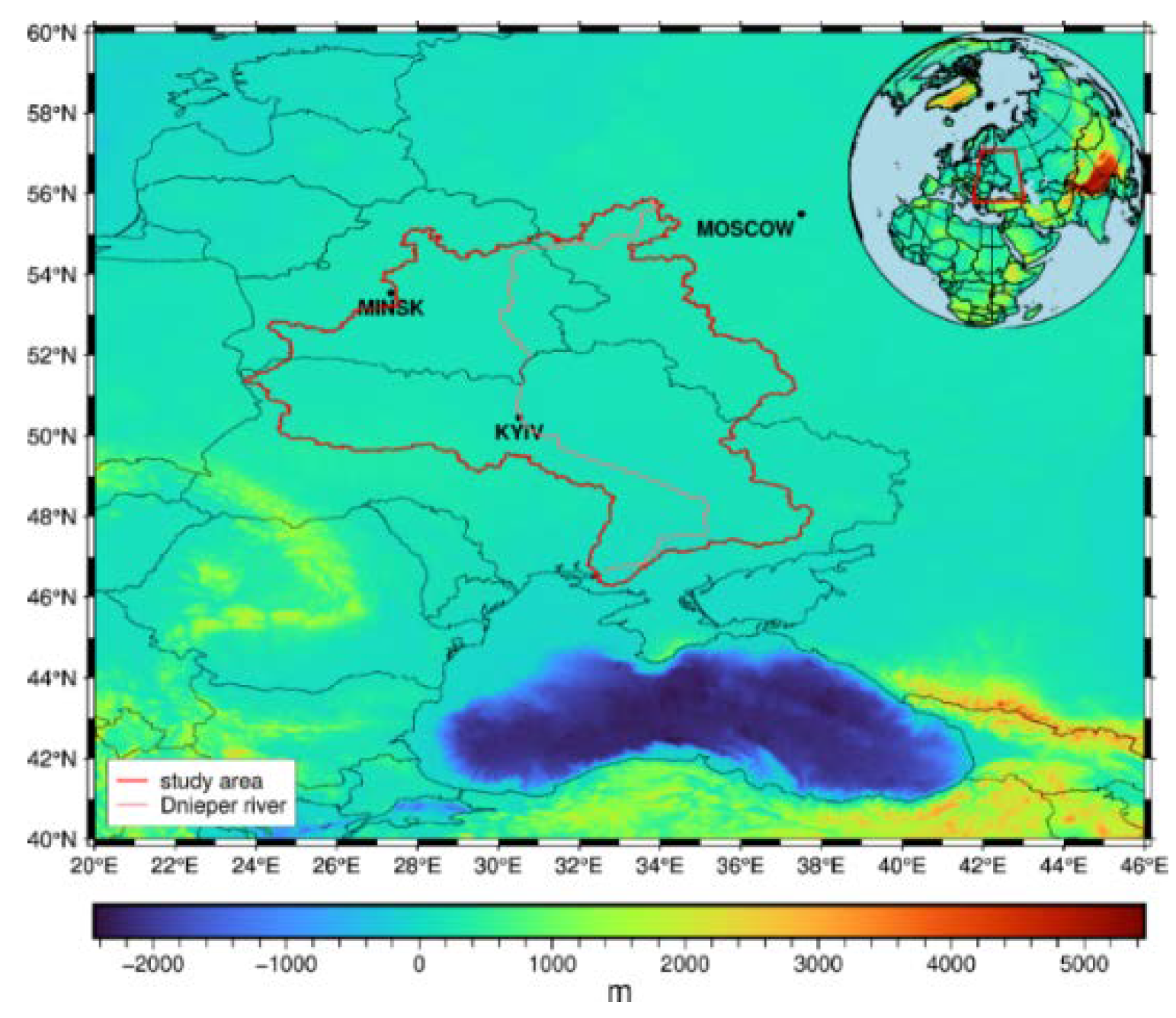
Figure 2.
The trend of TWS anomaly from forward modeling (Unit: mm/a). a) The initial mass rates of the Dnieper River basin from the results of GRACE observation with decorrelation and a 300 km Gaussian filter. b) Forward modeling ‘true’ mass rates of the Dnieper River basin after a 50 times iteration procedure with an acceleration factor of 0.6. c) The mass rates are handled with the same filter approach as a) computed from b). d) The difference in mass rate between a) and c).
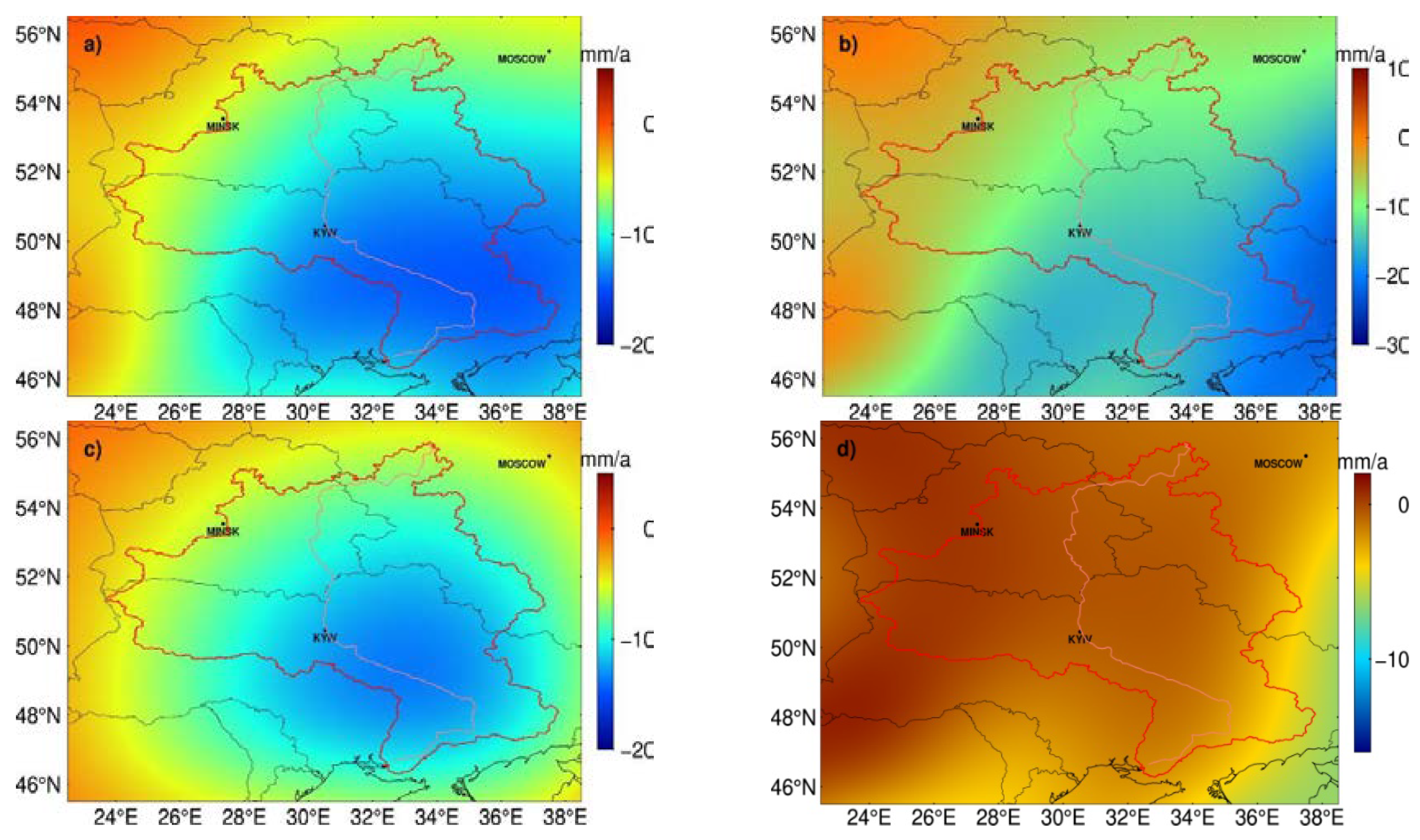
Figure 3.
GRACE time series of TWS anomaly that has been conducted with decorrelation and Gaussian filter (blue), Mascon time series (red) extracted from CSR RL06 Mascon Solutions (version 02), forward modeling (FM) ‘true’ time series modeled by a 50 iterate procedure (green), and forward modeling ‘true’ time series filtered with the same filters of GRACE (purple), the residuals time series between recovered and ‘true’ time series.
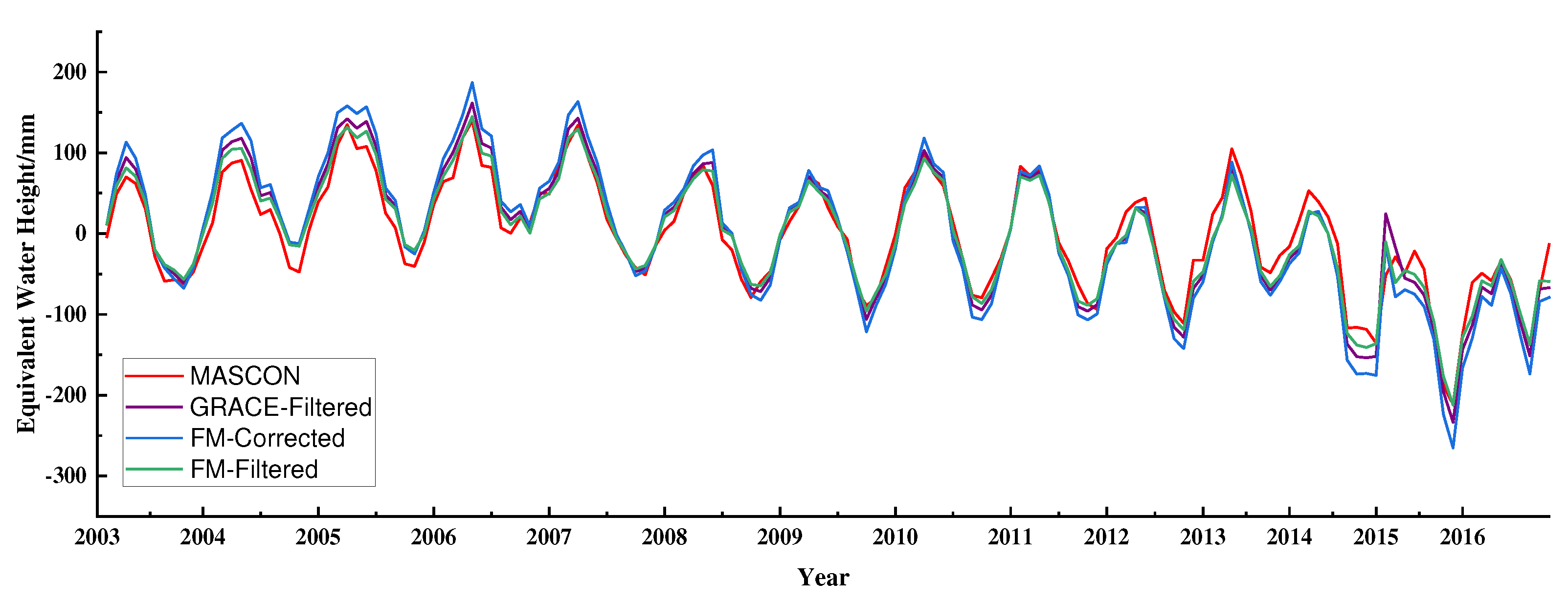
Figure 4.
GRACE time series of total water storage that has been conducted with decorrelation and Gaussian filter (purple), Mascon time series (red) extracted from CSR RL06 Mascon Solutions (version 02), forward modeling (FM) ‘true’ time series modeled by a 50 iterate procedure (green), and forward modeling ‘true’ time series filtered with the same filters of GRACE (purple), the residuals time series between.
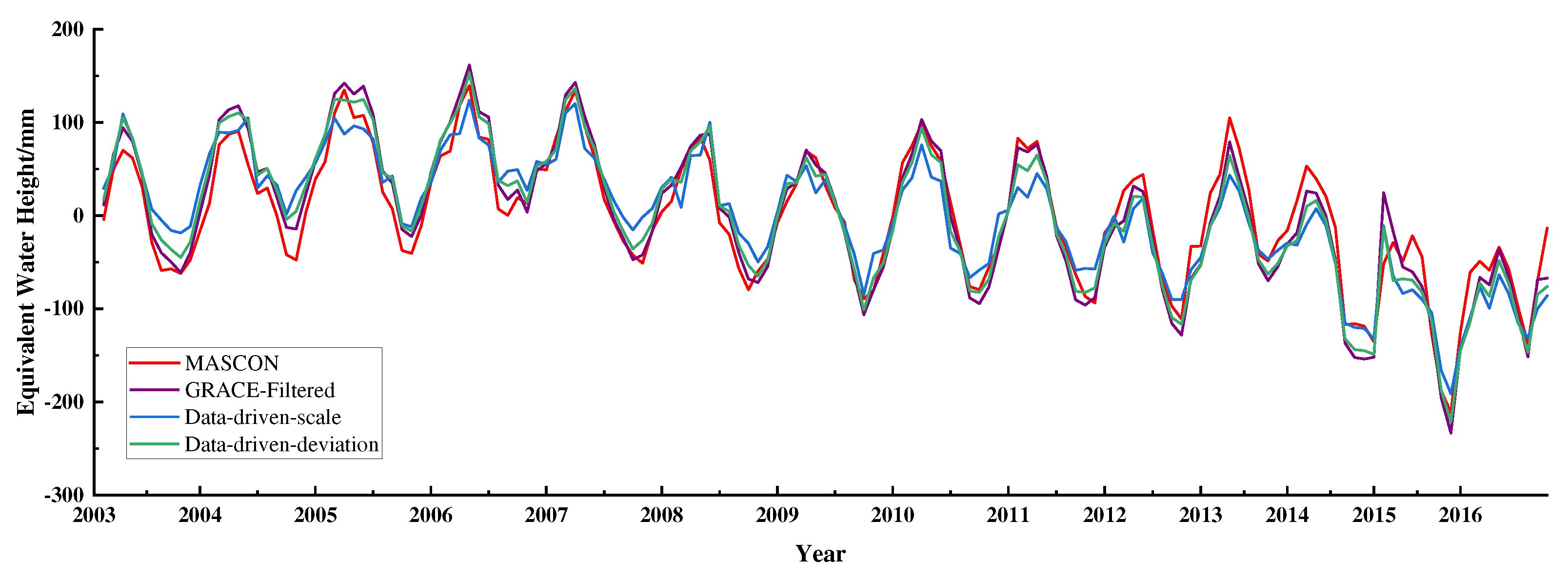
Figure 5.
The trend of TWS anomaly, (a) is GRACE filtered results, (b) is the recovered results by the single factor derived from WGHM, (c) is the recovered results by the single factor derived from GLDAS, (d) is the recovered results by the single factor derived from CPC.
Figure 5.
The trend of TWS anomaly, (a) is GRACE filtered results, (b) is the recovered results by the single factor derived from WGHM, (c) is the recovered results by the single factor derived from GLDAS, (d) is the recovered results by the single factor derived from CPC.
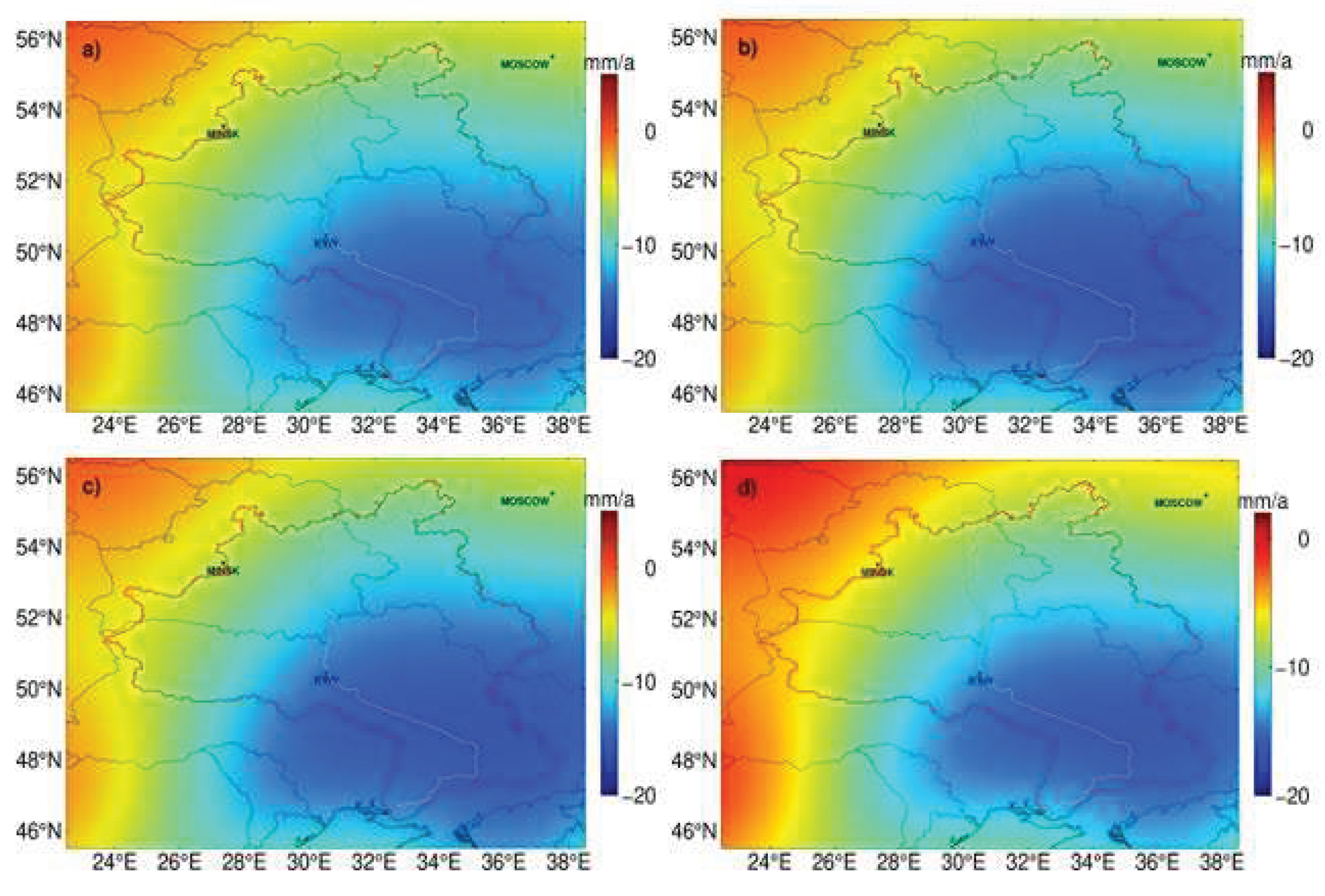
Figure 6.
The time series of TWS anomaly recovered by single factor approach, the ‘true’ time series for validation obtained from CSR MASCON products (red), the time series after the filter process, the time series recovered by a scaling factor calculated from the WGHM (green), and GLDAS (blue), and CPC (orange) models.
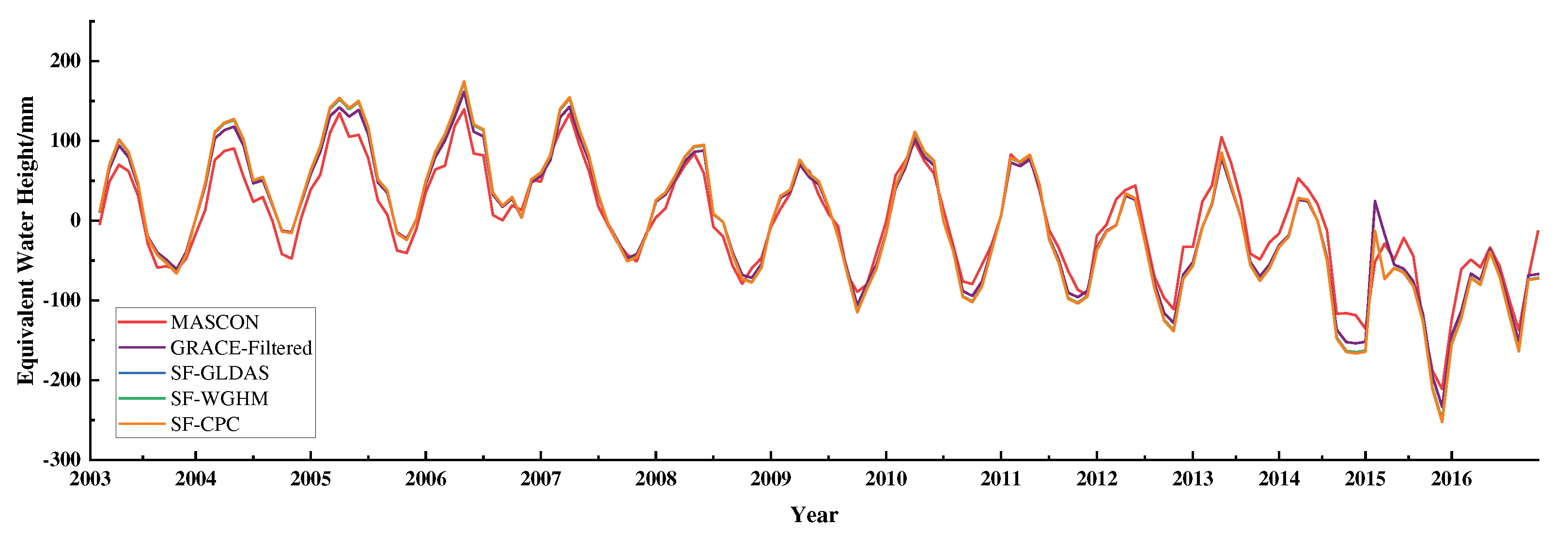
Figure 7.
The XWT of time series between GRACE time series of TWS anomaly and three-time series of TWS anomaly simulated from hydrological models. The first row is the results of XWT that GRACE filtered time series with unfiltered time series derived from WGHM, GLDAS, and CPC models; the second row is the results of XWT that GRACE filtered time series with filtered time series derived from WGHM, GLDAS, and CPC models.
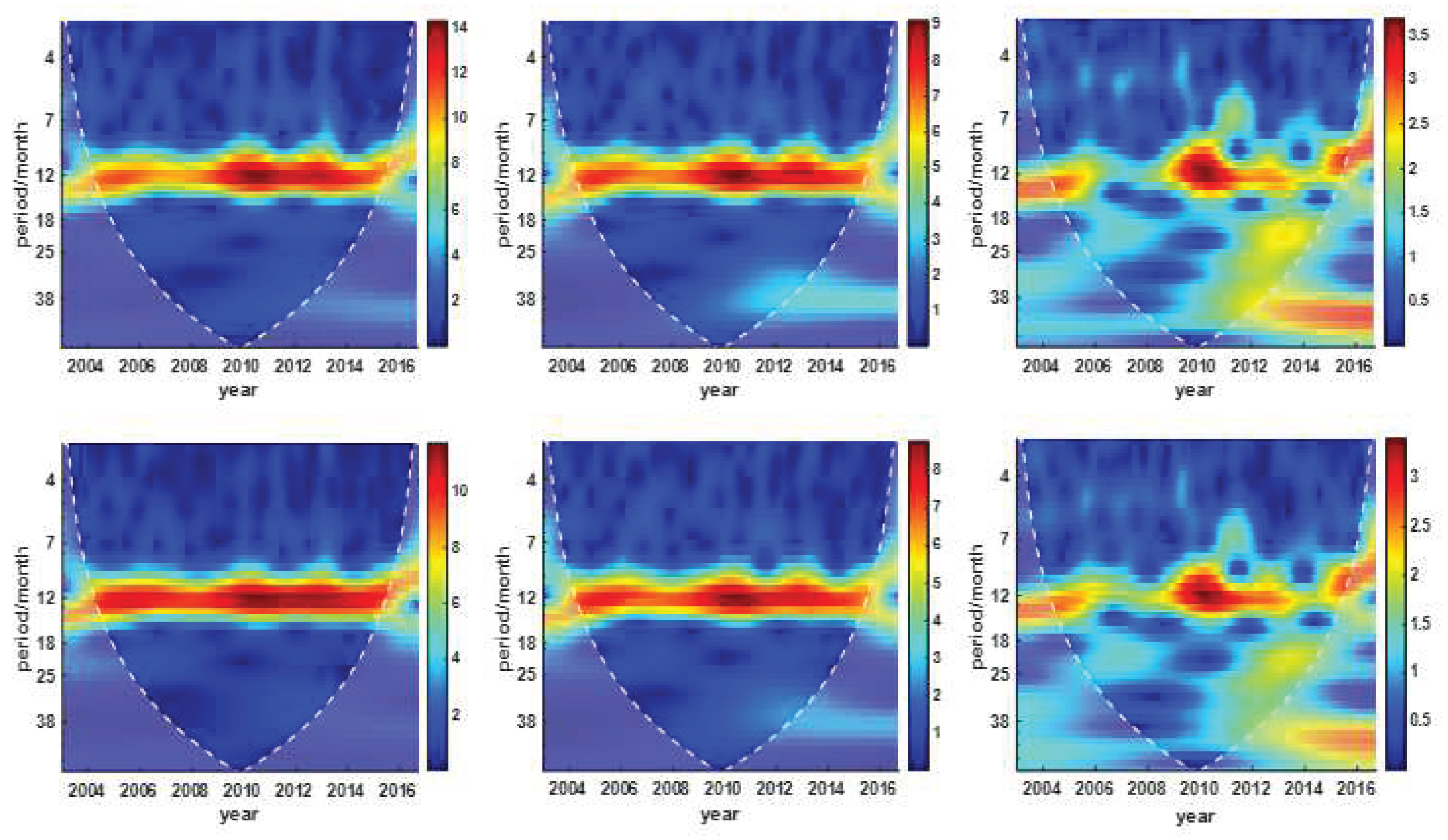
Figure 8.
The semi-annual amplitude variation of TWS anomaly in the Dnieper River basin that corrected by a multiple factor approach. (a) the semi-annual amplitude variation of TWS anomaly separated from the filtered GRACE results, (b) the one corrected by multiple factor approach based on (a).
Figure 8.
The semi-annual amplitude variation of TWS anomaly in the Dnieper River basin that corrected by a multiple factor approach. (a) the semi-annual amplitude variation of TWS anomaly separated from the filtered GRACE results, (b) the one corrected by multiple factor approach based on (a).
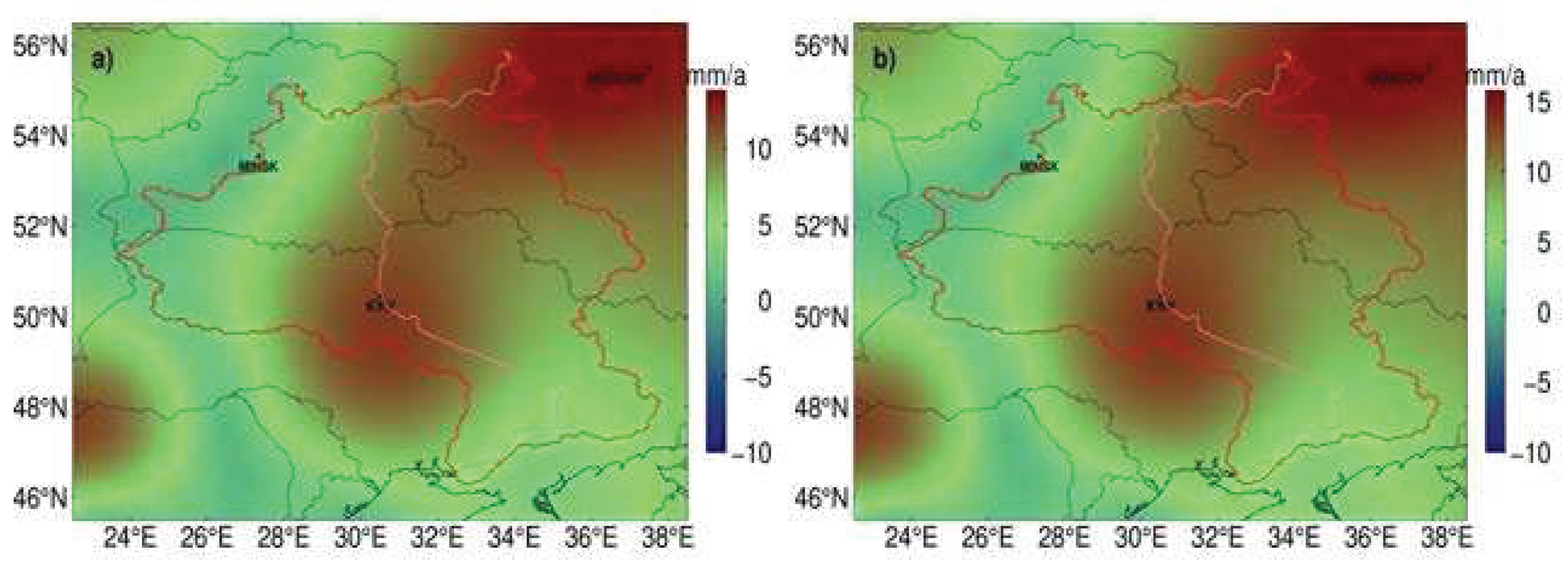
Figure 9.
The time series of TWS anomaly in the Dnieper River basin for multiple scaling factor approach.
Figure 9.
The time series of TWS anomaly in the Dnieper River basin for multiple scaling factor approach.
Figure 10.
The correlation of TWS anomaly between the obtained GRACE (solid line), CPC (dash line), and GPCC (bar).
Figure 10.
The correlation of TWS anomaly between the obtained GRACE (solid line), CPC (dash line), and GPCC (bar).
Figure 11.
The temperature anomaly of every February from 2003 to 2016 in the spatial domain.
Figure 12.
The temperature anomaly of August and September 2015 in the spatial domain.

Table 1.
List of the data sets.
| Data Name | Data Version | Resolution | Period | Data Access |
|---|---|---|---|---|
| GRACE | CSR, R06L2 | 96 degrees and orders, monthly | 2003- 2016 |
ftp://isdcftp.gfz-potsdam.de/grace-fo/ |
| Snow Water Equivalent | GLDAS Noah,version2.1 | 1°by1°,monthly | 2003- 2016 |
https://disc.gsfc.nasa.gov/ |
| Soil Moisture | GLDAS Noah,version2.1 | 1°by1°,monthly | 2003- 2016 |
https://disc.gsfc.nasa.gov/ |
| Total Water Storage | WGHM, Version2.2d | 0.5°by0.5°,monthly | 2003-2016 | https://doi.pangaea.de/ |
| Precipitation | GPCC, Full Monthly Version 2020 | 0.25°by 0.25°,monthly | 2003-2016 | https://opendata.dwd.de/ |
| Soil Moisture | CPC Soil Moisture V2 | 0.5°by0.5°,monthly | 2003-2016 | https://psl.noaa.gov/data |
Table 2.
Comparison of the Mascon time series and the reconstructed time series are derived from the different recovered approaches.
Table 2.
Comparison of the Mascon time series and the reconstructed time series are derived from the different recovered approaches.
| model | FM | Data-driven | SF | MF | |||||||||||
|---|---|---|---|---|---|---|---|---|---|---|---|---|---|---|---|
| — | R | NSE | R | NSE | k | R | NSE | K | R | NSE | K1 | K2 | K3 | R | NSE |
| — | 3.22 | 0.77 | 2.70 | 0.84 | 1.33 | 3.40 | 0.75 | — | — | — | — | — | — | — | — |
| WGHM | — | — | — | — | — | — | — | 1.073 | 2.61 | 0.85 | 1.23 | 1.02 | — | 3.09 | 0.79 |
| GLDAS | — | — | — | — | — | — | — | 1.072 | 2.60 | 0.85 | 1.11 | 1.06 | — | 2.64 | 0.85 |
| CPC | — | — | — | — | — | — | — | 1.082 | 2.66 | 0.84 | 1.02 | 1.04 | 1.14 | 2.32 | 0.88 |
Note. R denotes the RMSE errors (Unit: cm), NSE is Nash-Sutcliffe efficiency, k is the scale factor, and k1, k2, and k3 are the scaling factors for trend, annual and semiannual items.
Disclaimer/Publisher’s Note: The statements, opinions and data contained in all publications are solely those of the individual author(s) and contributor(s) and not of MDPI and/or the editor(s). MDPI and/or the editor(s) disclaim responsibility for any injury to people or property resulting from any ideas, methods, instructions or products referred to in the content. |
© 2023 by the authors. Licensee MDPI, Basel, Switzerland. This article is an open access article distributed under the terms and conditions of the Creative Commons Attribution (CC BY) license (http://creativecommons.org/licenses/by/4.0/).
Copyright: This open access article is published under a Creative Commons CC BY 4.0 license, which permit the free download, distribution, and reuse, provided that the author and preprint are cited in any reuse.


