Submitted:
02 August 2023
Posted:
03 August 2023
Read the latest preprint version here
Abstract
In this article, the Shannon entropy measure was used to evaluate the change in precipitation and temperature conditions. Due to the short, low-volume sequences of analyzed precipitation and temperature data, a bootstrap method was used in the procedure for calculating Shannon entropy. The analysis used minimum and maximum values of monthly precipitation totals and average monthly temperatures for 377 catchments distributed across the globe. 110-year data sequences from 1901 to 2010 were analyzed. Entropy values for the estimated parameters of the generalized extreme value distribution (GEV) were calculated for the accepted data. Entropy value calculations were performed for the left-hand constraint, based on minimum values, and for the right-hand constraint, based on maximum values. Based on the analysis of precipitation and temperature sequences, trend forms were identified for the left and right Shannon entropy values. This made it possible to obtain information on the directions of changes occurring in the area of minimum and maximum values in the field of monthly precipitation and average temperatures in the analyzed catchments. The study showed the existence of Shannon entropy trends. Evaluation of entropy trends for precipitation and temperature sequences was performed using non-parametric tests. Mann -Kendall tests at the 5% significance level were used in the trend analyses. The Pettitt test was performed to determine the point of change in trend for precipitation and temperature data. The analysis performed was supported by graphical presentations.
Keywords:
Shannon entropy
; bootstrap method
; GPCC data
; NOAA data
; monthly precipitation
; average temperature
; climate trends
; Mann Kendall test
; Pettitt test
1. Introduction
Climate extremes such as droughts, floods, extreme temperatures or storms have the potential to have a significant impact on economic sectors that are closely linked to climate, such as water management, agriculture, food security, energy security, forestry, health and tourism. Changes in these sectors could have far-reaching consequences for countries whose economies rely more heavily on these sectors [1,2,3]. Most previous research work on climate change, unfortunately, overlooks or downplays the importance of the variability of extreme climatic conditions. The variability of these characteristics is an important aspect of climate change risk assessment, as it affects the intensity and frequency of extreme events. The IPCC report points out [4,5,6] that expected changes in the variability of precipitation and temperature in the future will be characterized by a high degree of uncertainty. In light of these facts, there is a need to develop methods and algorithms that can improve the efficiency of predicting and estimating the intensity of climate hazards [3,7]. The Earth's atmospheric system is too complex to be described deterministically. This means that predicting its future state is difficult or impossible [8]. It is an open system and driven mainly by the continuous influx of solar radiation and the Earth's rotation. The system is too large to solve deterministically due to: the number of data needed to describe its state, incomplete instrumentation to monitor its state, the lack of a correct way to spatially partition the system for long-term analysis, and the lack of accurate historical data before 1900. Therefore, stochastic analyses can be useful in assessing the variability of climate conditions [8]. Analyses of entropy directions show that if global warming were to continue, a decrease in thermodynamic entropy would mean more free energy driving the weather; an increase in informational entropy would mean difficulty in predicting which way the process would go [8]. One potential tool to help with this is the Shannon entropy trend assessment. Entropy analysis can provide information on the degree of irregularity, unpredictability and variability in climate systems, which can be valuable for developing more accurate forecasts and strategies for managing risks associated with extreme climate events.
Climate change is a phenomenon that leads to significant spatial and temporal heterogeneity in the impact of these changes on biological systems, health and sectors of economies [9]. Studies show that global increases in average temperature mask significant differences in temperature increases between land and sea, and small areas and large regions [10,11,12]. Climate change also inevitably results in changes in the frequency, intensity, spatial extent, duration and timing of extreme weather and climate events [1,2,3]. One can analyze extreme values in the context of changes in the types and parameters of probability distributions, trends in statistical characteristics (e.g., minimum, maximum values) [13]. One can also look at the variation of extreme values through the characteristics of the tails of extreme distributions [14,15,16]. It is also possible to monitor the change in Shannon entropy and its trends as a measure of climate variability and the extremes following this variability.
Shannon entropy is a measure of the degree of disorder or unpredictability in a system, and an increase in entropy can indicate greater climate variability. Analysis of Shannon entropy and other measures of a statistical nature can be useful for assessing climate variability and extremes. This will enable a better understanding of the effects of climate change on different systems and take appropriate measures to adapt and reduce its negative consequences. Shannon entropy trend analysis of the climate system, taking into account the interaction between precipitation and temperature [2,17,18,19], is extremely important for several reasons. Positive feedback in the climate system can lead to an increase in entropy due to complex changes in precipitation and temperature. For example, an increase in temperature can increase the intensity of rainfall, which in turn leads to extreme flooding events. This phenomenon is amplified because more precipitation can also influence further increases in temperature, resulting in more rainfall.
Precipitation and temperature play a key role in the global energy and water cycle [17,20,21,22,23] and their variability can lead to floods, droughts and other natural disasters. Analysis of the variability of temperature and precipitation extremes is necessary because of their impact on many aspects of the natural and human environment. In the article, based on long-term sequences of precipitation and temperature, it is shown that the process of variability of minimum and maximum values, can lead to significant changes in the local environment. Such changes can affect the distribution of plant and animal species, weather patterns, agriculture and the economy, and many other aspects of the environment and life. Knowledge of the nature of the changes and the time scales of these phenomena is used to reduce the risks of all types of hazards, including floods and drought. Proper understanding of the nature of variability in extreme phenomena is key to developing strategies related to mitigation [12,24,25] and minimizing the impact of anthropogenic factors [25,26,27].
Projections indicate that as the planet warms, climate and weather variability will increase. Changes in the frequency and intensity of extreme climatic events and in the instability of weather patterns will have significant consequences for both human and natural systems. By the end of this century, the frequency of extreme conditions, such as heat stress, droughts and floods, is expected to increase, with numerous negative impacts beyond those resulting from changes in average values alone [1,2,3]. Given the uncertainty associated with forecasts of changes in extremes and the limited confidence in these forecasts, it is important to conduct trend analyses and extreme value analyses based on the longest possible measurement sequences. Both the low certainty of forecasts and the high confidence in them do not exclude the possibility of extreme changes. In the context of limitations in understanding climate processes in different regions, there is a possibility of extreme changes with low probability, however with significant impact. Changes in extremes are observed, and there is evidence that some of these changes are due to anthropogenic influences [1,2,3]. Analysis of historical observations of climate variables indicates anthropogenic changes in climate [28,29,30]. The study of changes in the amount of precipitation and temperature variability [16,31,32,33,34,35], depending on the observed period, show changes in trends and allow us to assess the form of the directions of these occurring changes [36,37,38,39]. However, attributing individual extreme events to these influences remains a challenge. An example of this is the analysis performed as part of the work on climate variability at different periods and scales in a given region (e.g., in the rhythm of multi-decadal oscillations) [40,41]. It has been noted that precipitation variability in Europe is mainly influenced by the ocean-atmosphere circulation, especially the North Atlantic Oscillation (NAO). Consequently, the complexity of ocean-atmosphere interactions makes it difficult to detect the main driving forces of the oscillation and their influence on the variability of extreme events in the region [42]. Finally, the observed changes in the magnitude, frequency and timing of extreme events obtained represent one of the first analyses of this under-researched phenomenon where patterns have been shown to be complex and not always consistent with previous studies [6,19,28,43].
Despite the existence of limitations and uncertainties regarding climate variability projections and their impact on biological systems, health and sectors of economies, the need for adaptation measures cannot be underestimated. There is a pessimistic forecast of future weather and climate variability on short time scales and large spatial scales [44]. There is an increase in the frequency and intensity of climate hazards. Phenomena resulting from climate variability are not only becoming more common, but also their intensity is increasing by shortening the duration of these phenomena. In addition, it is possible to observe a change in the direction of the phenomena in the short term and the dynamics of extreme values [45]. Minimizing the impact of increasing climate risks requires a combination of climate-influencing actions and adaptive capacity in the planning process [44]. Assessments indicate an increased likelihood of future critical events, partly due to positive feedbacks in the climate system [46]. The impacts of these events are estimated to be large, making the risks significant [47]. Therefore, despite current limitations and uncertainties, there is an urgent need for adaptation measures to minimize the impact of increasing climate risks on various economic sectors, health, security and biological systems.
The increase in entropy affects the unpredictability of the weather and makes it difficult to plan adaptation activities. There can be a sudden transition from one extreme state to another in a short period of time. An increase in entropy in the climate system increases the degree of chaos and unpredictability. This, in turn, leads to greater weather variability, more frequent occurrence of extreme climatic events and difficulty in predicting long-term trends. Increased entropy can negatively affect economic sectors, such as agriculture, which need stable weather conditions for efficient production. However, increased entropy can also lead to greater biodiversity, as organisms must adapt to more variable environmental conditions. In the climate system, there is a complex interaction between polarization feedback [45] and increased entropy. Polarization feedback refers to the change in direction and intensity of climate phenomena over a short period of time. Abrupt jumps between weather extremes, such as sudden changes from drought to torrential rains or from extreme cold to heat, are examples of polarization feedback. The feedback of polarization and entropy increase is that the phenomena reinforce each other. Rapid changes in weather, characteristic of polarization, can contribute to greater weather variability and an increase in entropy. In turn, an increase in entropy can affect larger jumps between extreme weather states, further intensifying polarization. Therefore, understanding positive feedbacks in the climate system, polarization and entropy in the climate system can be important to better understand climate change and develop effective management and adaptation strategies. The interactions of climate variables can affect the occurrence of hurricanes, tornadoes and droughts. In addition, these interactions can affect a measure of risk that includes threats to life, livelihoods, health, well-being, ecosystems, species, economic, social and cultural resources, as well as services (including ecosystem services) and infrastructure. Risk results from the interaction between system vulnerability and exposure, and between system exposure and forcing [10,18,48]. As a result, one phenomenon can amplify or weaken another, complicating the process of understanding the scale of climate change. Anthropogenic factors, such as industrial activity, deforestation, land use transformation, pollutant emissions and greenhouse gas emissions [17,26,27,49,50], can affect the variability of extreme values and polarization of climate factors [10,45,51,52,53].
Shannon entropy finds application in climate change analysis by enabling the measurement of the degree of disorder and complexity of climate change distributions. It can help identify trends, cyclicality, fluctuations and anomalies in climate data, as well as forecast future changes based on historical data. It can be used to analyze various aspects of climate, such as variability in temperature, precipitation, wind variability, water levels, etc. The application of Shannon entropy can also help evaluate the effectiveness of measures to reduce human impact on climate, such as reducing greenhouse gas emissions, changing land use and crop types, changing agri-food production and its spatial distribution, types of industrial infrastructure, and developing renewable energy sources. In this way, Shannon entropy can be useful in scientific research, climate policy and planning for environmental protection.
2. Methodology
Today, there is a growing body of scientific evidence confirming that human activities are influencing climate change, contributing to shorter durations of high-intensity precipitation and longer periods of high temperature and low precipitation. The variability of extreme events, such as floods and droughts, is increasingly apparent and can be attributed to the erratic nature and intensity of human activities. Therefore, the study of climate variability factors related to monthly precipitation and average monthly temperatures is key to understanding climate change at the regional level and developing strategies to manage water resources and reduce the risk of floods and droughts.
The minimum and maximum values of monthly precipitation and the minimum and maximum values of average monthly temperatures during the year were adopted for the analysis. In view of the purpose of the analysis, i.e. assessing long-term climate variability, it is better to perform analyses on averages rather than on extreme values for several reasons. Such analyses have greater statistical stability. Averages have less variability than extreme values, which means that for the same data we will get a smaller standard error of the average estimator than of the extreme value estimator. Statistical stability is particularly important for long-term analyses, since variability in values can affect the interpretation of results and decision-making. Another argument is the larger number of observations, since analysis on averages can be performed for a larger number of observations than analysis on extreme values, allowing for more representative results. It should be noted that analyses on averages are a better reflection of reality, allowing to obtain information on typical values, which are more representative of long-term changes than extreme values. In addition, extreme values can be the result of random factors or unpredictable events that do not reflect typical conditions. In summary, for the search for long-term changes, analysis on averages is more statistically stable, allows for a larger number of observations, and better reflects typical values, which is important for decision-making and action planning.
Calculations of Shannon entropy variability were made for the "left tail" based on the following, respectively: minimum values of monthly precipitation and minimum values of average monthly temperature. For the "right tail," calculations of Shannon entropy variability were made for, respectively, on the basis of maximum values of monthly precipitation and maximum values of average monthly temperature. Due to the small-volume dataset, a bootstrap technique [54,55,56,57,58] was used to evaluate the distributions of extreme values of minimum and maximum values of Shannon entropy variability. It should be noted that for the evaluation of the "left tail" parameters, distribution parameters estimated based on minimum values were taken, while for the "right tail" distribution parameters were estimated based on maximum values.
3. Bootstrap Resampling Technique
In the present study, a bootstrap resampling technique was used to estimate the parameters of the distribution of extreme precipitation and temperature values.. The main idea of bootstrap is to generate large samples with replacement by resampling the original samples based on the assumption that the samples are independent and identically distributed. This method is recommended not only for its computational efficiency, but as an easy-to-implement approach that generates bootstrap replications without relying on the assumption of true distribution [58]. It can be implemented by relying only on the information obtained from the sample value.
The steps of the bootstrap method used in this study are described as follows:
-
population sequences of annual minimum and maximum values from monthly precipitation and annual minimum and maximum values from monthly average temperatures were created:
- -
- for the left tail:
- -
- for the right tail:
The number of elements in both the precipitation and temperature sequence does not reliably assess the value of the probabilities of events classified in the left and right tails. A 1000-fold number of draws from the 70-element sequence was assumed. Since the possibility of assessing Shannon entropy trends was assumed, it was assumed that the 70 element strings would be created in the following recursive manner:
for the left tail
- -
- for the right tail:
Thus, forty 70-element strings were arbitrarily obtained. These strings constituted a resource for 1000-fold bootstrap drawing. In this way, 40 sequences 1000 times drawn by the bootstrap method were created on the basis of which Shannon entropy was calculated for both precipitation and temperature for minimum and maximum values.
- 2.
- it was assumed that the series of annual minimum and maximum monthly precipitation and average temperature were original samples, the total length of multi-year records.
- 3.
- bootstrap samples of the minimum and maximum series of precipitation and temperature were drawn using the bootstrapping process, which involves randomly selecting values to replace the original sample.
- 4.
- the above analysis was carried out on all analyzed catchments.
For each, drawn string, the Anderson-Darling test (ADT) was performed to confirm the possibility of describing the drawn string with the generalized extreme value distribution (GEV) distribution at the 5% significance level. Otherwise, the results of such an experiment were not taken into account, proceeding to the next draw. For the estimation of the parameters of the "left tail" of the GEV, the compliance of the ADT test at the 5% significance level was achieved at 91%, for the "right tail" at 99.6%. In the next step, the parameters of the generalized distribution of extreme values were estimated using the maximum likelihood method [57,59,60,61].The ADT test was adopted because of the priority given to values from the tails of the distribution, which is important for extreme distributions. In subsequent steps, the value of Shannon's entropy estimator was calculated at a significance level of 5% [55]. The above methodology was applied to each of the 377 catchments analyzed. The analysis code was developed in Matlab software.
4. Fitting the GEV Distribution
Modeling the variability of climate extremes requires accounting for extremes in such phenomena as precipitation, temperature, evaporation, atmospheric pressure and others [62]. In modeling extreme values, an approach that uses a sequence of observations extracted from equal periods, such as a maximum from monthly totals or a minimum from monthly precipitation totals for a given year, is widely used. Similarly, for a maximum from average temperatures or a minimum from average temperatures for a given year, it assumes that the set of extremes is independent and identically distributed, being fitted to a probability distribution model such as the generalized extreme value distribution (GEV). As the impact of climate change has become an important issue, many efforts have been made to account for non-stationarity in hydrological applications. One popular approach is to apply various non-stationary models to non-stationary data and select an appropriate model based on model diagnostics. Due to its adaptability to changes in the data structure, non-stationary model parameter estimation based on maximum likelihood is usually used for this purpose [57,60,61,63]. To date, this approach has been widely studied and can be described as a "user-friendly" method. However, from a statistical point of view, there is a problem regarding ergodicity in non-stationary extreme value modeling [55,64].
The ergodicity assumption is often used in time series analysis because it allows the use of statistical methods that require independence of samples. Thus, it is possible to infer the properties of time series from a single realization. However, it is important to note that the ergodicity assumption can be a simplification that is not always met in practice. Time series can be composed of various factors, such as trends, seasonality, cyclicality or jumps, which can violate ergodicity [65,66]. To account for these non-standard properties of time series, other approaches such as autocorrelation analysis, power spectral density analysis [43,67], or spatial temporal dependence analysis are also used in practice. Although the assumption of ergodicity is often used in the statistical analysis of time series, caution should be exercised and other methods should be considered, which can take into account the specific properties of the series under study [57,64],
The aforementioned approach, for non-stationary hydrological data, based on the estimation of parameters of a non-stationary model, based on the highest reliability, is one of the most commonly used in practice. However, when dealing with extreme values, the problem of ergodicity can introduce additional difficulties in data analysis. Ergodicity refers to the property of a stochastic process that is equivalent in its behavior in a statistical sense, no matter what time points are observed. In the case of non-stationary processes, such as climate change, it cannot be assumed that extreme values will have the same statistical properties over time. This is why with non-stationary processes, including climate change, ergodicity-based approaches can lead to incorrect statistical conclusions. One solution is to use non-stationary models that take into account the non-stationarity of the process. It is also necessary to use appropriate statistical tools, such as hypothesis tests, that account for nonstationarity in the data. Despite the fact that nonstationarity is already widely taken into account in climate change research, the problem of ergodicity in extreme data analysis still needs research attention [55,57,64].
The parameters refer to the shape parameter, scale and position [68].
5. Shannon Entropy
Shannon's entropy measures the indeterminacy and unpredictability of information. In the case of climate change, entropy can help analyze the various factors influencing climate change and predict its effects in the future. It can help identify changes in atmospheric conditions, such as changes in temperature, precipitation and pressure, that may affect climate change. Entropy can also help analyze complex interactions between different climate factors, such as atmospheric circulation, ocean circulation and the amount of solar radiation. It can also be used to assess the risk of climate change, in evaluating the probability of different climate change scenarios and in determining the degree of uncertainty associated with these scenarios. In addition, entropy can help identify different patterns of climate change, such as climate cycles in which periodic changes in solar radiation and ocean circulation affect climate change. Entropy can also be used to determine the complexity of the climate and its systems, which can help understand how different factors affect climate change. Finally, entropy analysis can help develop strategies to manage the risks associated with climate change, which is particularly important as the number of climate change-related disasters such as hurricanes, floods and droughts increases. Shannon entropy finds application in climate change analysis by enabling the measurement of the degree of disorder and complexity of climate change distributions. It can help identify trends, cyclicality, fluctuations and anomalies in climate data, as well as forecast future changes based on historical data. It can be used to analyze various climate factors and evaluate the effectiveness of measures to reduce the impact of human activities on climate.
The groundbreaking work of C.E. Shannon, considered the founder of mathematical information theory, stating that the most representative of information processes, as processes that reduce uncertainty, is the expected amount of information understood as the entropy of the source [8,55,70]. The concept of entropy has been used in the study of physical systems, and was defined on the occasion of the second law of thermodynamics. The measure of entropy defined by C.E. Shannon on the basis of information theory has been applied in subsequent years in many scientific fields, including statistics and computer science. Today, information theory is still mainly concerned with communication systems, but applications of the concept of entropy in the analysis of the behavior of a variety of systems, including economic and social systems, financial systems, climate systems are emerging, and subsequent years have brought numerous generalizations of Shannon's measure of entropy [8].
In information theory, the definition of the entropy measure of a random variable with a discrete distribution { is preceded by the formulation of conditions for the entropy function:
The conditioning system proposed by Shannon assumed that entropy should satisfy the following conditions:
- the function should be continuous with respect to all probabilities which means that small changes in probabilities should correspond to a small change in entropy.
- if all n events of random variable X are equally likelythen the function should grow monotonically as n increases.
- The function should be symmetric, which means that the entropy value is invariant to the permutation of the probabilities
- The function should be coherent, which means that if the realization of events takes place in two consecutive stages, the initial entropy should be a weighted sum of the entropies of each stage. There is exactly one [71], with constant -variable function satisfying the above conditions, and it is given by the formula:
The constant determines the unit of entropy. If the unit of entropy is the bit and the entropy function takes the form:
Entropy is a measure of the uncertainty associated with the probability distribution with which the values of the discrete variable X occur.
The probabilistic entropy measure described by the formula has the following properties:
- Shannon entropy takes non-negative values ,
- Shannon's entropy takes the value zero when one of the values of the discrete random variable occurs with probability equal to unity, and the others with probabilities equal to zero,
- Shannon entropy takes the largest value equal to when all probabilities are equal to each other ,
- Shannon's entropy is concave,
- Shannon entropy satisfies the additivity property for a pair of discrete independent random variables and :
In the present study, Shannon entropy values were calculated for the values of extreme monthly precipitation totals and extreme monthly mean temperatures. The sequences thus created provided data for further analyses related to the evaluation of entropy dynamics.
6. Variability of entropy
In the paper, entropy was calculated separately for minimum values and maximum values. A measure was proposed to take into account the variability of distributions describing extreme values. The evaluation of the variability of Shannon entropy was made on the basis of the values of calculated trends. A measure of the Euclidean norm was proposed here [72,73,74,75,76].
The Euclidean norm can be written as:
where:
- - coordinates of the vector
In this study, the variability was determined based on Shannon entropy trends separately in the form of distributions describing minimum values and distributions describing maximum values. Finally, it also allowed calculating the resultant variability of Shannon's entropy by taking the entropy trends for precipitation phenomena and temperature phenomena separately as vector coordinates. Finally, a measure was proposed that takes into account the variability of both precipitation and temperature extremes.
where:
– Shannon entropy trend for minimum rainfall values,
– Shannon's entropy trend for maximum rainfall values,
– Shannon's entropy trend for minimum temperature values,
– Shannon's entropy trend for maximum temperature values,
– variation of Shannon's entropy for extreme precipitation values,
– variation of Shannon's entropy for extreme temperature values,
– variation of Shannon's entropy for extreme values of precipitation and temperature.
The Euclidean norm is one of many ways to measure the dynamics of climate variability, and its calculation based on Shannon entropy trends for temperature and precipitation extremes can help understand climate variability. It can be used to compare different time periods and geographic regions to assess whether the dynamics of climate variability are increasing, decreasing, or remaining constant. However, the Euclidean norm itself does not provide insight into the causes of these changes, but only informs about the degree of variability itself. It is worth noting that calculating the Euclidean norm from Shannon's entropy trends for minimum and maximum temperature and precipitation values is one of many possible ways to analyze climate entropy variability, and should be considered as a complement to other research methods, not as the only method of analysis.
7. Data Preparation for Analysis
The paper relies on grid data of monthly precipitation totals from the Global Precipitation Climatology Center (GPCC) released products and grid data of monthly mean temperatures from National Oceanic and Atmospheric Administration (NOAA) products. The data correspond to a spatial resolution of 0.5°x 0.5° and are consistent in spatial and temporal extent. Products from both GPCC and NOAA are made available via the Internet [77,78,79,80]. These data are not made available in real time.
This paper examines global Shannon entropy trends of monthly precipitation totals and monthly mean temperatures from an area of 377 river basins distributed over all continents. Assuming 509.9 million square kilometers of land area, 12.76% of the land area is included in the analysis. Table 1 shows the areas covered by the analysis.
GPCC and NOAA data, were converted to catchment areas. This yielded a sequence of monthly precipitation and temperatures, which became the subject of the analyses presented in this article. The analyses covered the years 1901 to 2010.
8. Statistical Tests Used
In evaluating the form of entropy trends for both precipitation and temperature, a bootstrap resampling technique was used to create sequences for calculating Shannon entropy and estimating GEV distribution parameters. The form of the trends was verified with the Mann-Kendall test (MKT) at the 5% significance level. In addition, entropy trend change points were determined using the Pettitt change point test (PCPT) at the 5% significance level. If the change point was positively verified at the 5% level of significance, a new trend form was determined for the new sub-series using the MKT test. The possibility of using the GEV distribution, for each, analyzed sequence of extreme values, the AD test was carried out at the 5% level of significance.
To examine the trend in a given time series, the MKT test was used [81,82]. This test is independent of the type of distribution and we do not need to assume any special form of data distribution function [83]. This test has been widely recommended by the World Meteorological Organization for public use, moreover, it has been used in many scientific papers to evaluate the trend of water resources data [13,29,82]. The magnitude of the trend is estimated using a nonparametric median-based slope estimator proposed by Sen [84] and extended by Hirsch [85]. In this study, this test was used to examine the Shannon entropy trend.
A number of methods [13,43,82,86,87], can be used to determine time series change points. In this analysis, the nonparametric Pettitt change point test [88] was used to detect the occurrence of change. The Pettitt change point test (PCPT) is a nonparametric abrupt change test in a time sequence. It is used to detect the turning point at which a sudden change occurred, the so-called "spike" in the time sequence. The TP involves comparing the sum of the ranks of two subsets of data, which are divided by a threshold value, to determine whether there is a statistically significant change in the time sequence. This test can be used to analyze data with any distribution, and the test result does not depend on the assumption of normality of the data. The result of the Pettitt test is the value of the test statistic, which is compared with the critical value for the significance level to determine whether the null hypothesis of no abrupt change in the time sequence can be rejected.
PCPT is widely used to detect changes in observed climatic as well as hydrological time series [13,89,90,91]. In the present study, the existence of change points in the Shannon entropy time series for extreme values of monthly precipitation totals and monthly mean temperatures was checked. For time series showing a significant change point, the trend test was applied to the sub-series, and if the change point is not significant, the trend test will be applied to the entire time series [13].
9. Analysis of Shannon’s Entropy Trend Variation
The study of Shannon entropy trends of extreme precipitation and temperature values is an important tool in the study of climate variability, which has important implications for hydrology and water resources [15,28,30,33,92]. Analysis of historical observations makes it possible to accurately assess the variability of precipitation and temperature according to the observed period and allows us to determine the form of the directions of these ongoing changes. Shannon entropy trends allow detection of trends and changes in these trends in extreme data. This makes it possible to accurately determine the impact of climate change on the environment and water resources. Studies of the variability of extreme values of precipitation and temperature are particularly important in the context of predicting the effects of hydrological floods and droughts, which can have serious consequences for humanity and the environment [28,29,30,51]. The use of statistical techniques, such as Shannon entropy trend analysis, makes it possible to more accurately predict these effects and take appropriate preventive measures. Finally, the use of statistical techniques in the study of climate variability is particularly important in the context of predicting the variability of extreme events [14,28,56,93,94,95,96,97]. Shannon entropy trends allow for a more accurate analysis of these phenomena and allow for an understanding of their causes and effects. This allows more effective action to protect the environment and water resources. They are important measures of climate variability, and their analysis makes it possible to understand the complex relationships between these two variables. Knowledge of entropy variability and the relationship between precipitation and temperature can allow us to understand the magnitude of atmospheric phenomena such as El Niño and La Niña cycles. In addition, the analysis of the interrelationships between these variables is important for assessing the polarization of climate phenomena and enables measures to be taken to reduce the negative effects of climate change.
The Intergovernmental Panel on Climate Change (IPCC) predicts that increased greenhouse gas emissions following the industrialization of the world, due to large-scale burning of fossil fuels, human interference and land use change, will increase global temperatures [18,27,30,98]. Natural forces and human activities contribute significantly to changing climate patterns, i.e., increasing land and ocean surface temperatures, changing spatial and temporal patterns of precipitation, increasing the frequency of extreme events, rising sea levels and intensifying El Niño [12,15,30,31,79]. Rapid changes, both in mean and variance, can be associated with both climate (e.g., shifts in climate regimes) and anthropogenic effects (e.g., construction of dams and reservoir systems, changes in land use/land cover and agricultural practices, relocation of measurement points) [10,99]. Statistical analyses must be interpreted in conjunction with observed physical [30,100,101], social and economic phenomena [30,34,102,103]. Therefore, the study and prediction of temporal trends in the entropy of extreme precipitation and temperature values is very useful in social and urban planning [104].
Analysis of the variability of Shannon entropy for GEV distributions of minimum and maximum values of precipitation and temperature can provide important information on the temporal variability and occurrence of extreme events caused by climate change [39]. Shannon's entropy is a measure of uncertainty or variability in the data distribution, meaning that the higher the entropy value, the greater the variability in the data distribution. In the case of climate change, an increase in Shannon entropy can indicate increasing variability in climatic conditions and more extreme events. In addition, a comparison of Shannon entropy values for minimum and maximum values of precipitation and temperature can provide information on the variability and polarization of extreme events.
This paper focuses on the variability of Shannon entropy in long-term sequences of precipitation and temperature to assess the polarization of climate phenomena. Shannon's entropy was used as a measure of the indeterminacy and unpredictability of climate phenomena: precipitation and temperature, which made it possible to study the degree of variability of these sequences over time. An increase in Shannon entropy in precipitation sequences indicates increased variability in precipitation and potentially extreme weather events, such as intense rains or droughts. Conversely, an increase in Shannon entropy in temperature sequences signals increased temperature variability and the potential for extreme events such as heat waves or extreme cold. Analysis of the variability of Shannon entropy makes it possible to identify areas where the climate is becoming more polarized. Higher entropy values indicate greater climate variability and unpredictability, which can lead to significant changes in the local environment. These changes include shifts in the distribution of plant and animal species, changes in weather patterns and changes in sea level [24]. Shannon entropy calculations of long-term precipitation and temperature sequences are extremely important in studying climate variability and assessing the polarization of climate phenomena. They allow a better understanding of climate dynamics and identify areas of greater variability and unpredictability.
The variability of entropy trends is one of the key indicators of climate change, and its analysis can help understand future changes in precipitation and temperature. A decrease in entropy trends for precipitation may suggest that the region is experiencing periods of drought or extreme precipitation, which could result in flooding. An increase in entropy trends for precipitation can indicate greater variability in the amount and timing of precipitation, which can lead to difficulties in managing water resources. Variability in temperature entropy trends can affect plant development, biological processes and animal migration [105,106]. A decrease in temperature entropy trends may suggest a more stable climate, but at the same time may lead to a lack of adaptation of organisms to changing conditions. An increase in temperature entropy trends can indicate increasingly unstable climate conditions, which can lead to the risk of extreme weather events such as heat waves or storms.
The study of the entropy trend change point, that is, a change in the direction or nature of precipitation and temperature trends, can be the result of various atmospheric factors and phenomena. This study does not analyze the causes of changes in the direction or nature of trends. On the other hand, it is possible to note in general terms what causes may cause this change:
- changes in atmospheric circulation: changes in atmospheric circulation, such as changes in winds, atmospheric currents or high and low pressure systems, can affect local precipitation patterns [108],
- changes in ocean surface temperature: ocean surface temperature is an important factor affecting regional precipitation patterns, ocean temperature anomalies such as El Niño and La Niña can affect precipitation changes [109],
- urbanization: urban development and land use changes can affect local precipitation patterns through the so-called "heat island effect" and changes in air circulation [52],
- global climate change: climate changes related to human activities, such as greenhouse gas emissions and global warming, can affect changes in precipitation patterns on global and regional scales [52],
- ocean-atmosphere interactions: changes in ocean-atmosphere interactions, such as ocean currents and the phenomenon of deep ocean upwelling, can affect regional precipitation patterns [52],
- industrial development: the growth of industrial activities, particularly greenhouse gas emissions and air pollution associated with industrial activities, can affect climate change and precipitation patterns. Emissions of greenhouse gases such as carbon dioxide (CO2) and methane (CH4) cause global warming, which can affect regional precipitation patterns, in addition, air pollutants emitted by industry can affect cloud formation and rain [53],
- agricultural development in particular changes in land use, can affect local precipitation patterns, excessive deforestation and changes in soil use can affect air circulation and moisture, which can affect local precipitation patterns, in addition, fertilization and irrigation practices in agriculture [52,53],
- other natural factors: in some cases, changes in temperature trends can be the result of natural climate changes, such as solar-magnetic cycles, changes in ocean circulation [21].
10. Results of the Analyses and Discussion
In the present study, Shannon entropy trends were examined on the basis of long-term sequences of monthly precipitation totals and monthly mean temperatures for 377 catchments from the area of 6 WMO regions. From the analyzed data, sequences of minimum and maximum values of precipitation and temperatures were selected. In evaluating the form of entropy trends for both precipitation and temperature, the bootstrap resampling technique was used to create Shannon entropy sequences and estimate GEV distribution parameters. The form of the trends was verified with the MKT test at the 5% significance level. In addition, the change points of the entropy trends were determined using the PCPT test at the 5% significance level. If the change point was positively verified at the 5% significance level, a new trend form was determined for the new sub-series using the MKT test. The applicability of the GEV distribution, for each, analyzed sequence of extreme values was evaluated using the ADT test at the 5% significance level. The results of the analyses were presented graphically. Graphical presentations of each aspect of the analysis performed allow easier and more precise observation of the trend of changes.
Figure 1 shows the Shannon entropy trends for the values of minimum monthly precipitation totals. The least negative values of entropy trends for minimum monthly precipitation values occurred in the river catchments shown in Table 2. It should be emphasized that in the catchment of the Daule River: Ecuador, the decreasing trend worsens, almost doubling from a value of (-0.040) to (-0.074). The turn of 1980/1990 is a period of changing trends.
Fewer extreme drought or intense rainfall events can be expected in these catchments, which can have a positive impact on agriculture and water resources. Lower entropy for minimum precipitation may indicate more predictable precipitation patterns, which facilitates water resources planning and management.
The largest values of entropy trends for the minimum values of monthly precipitation occurred in the river catchments shown in Table 3. It should be noted that in the catchment of the Anyuy River: Russian Federation there is a decrease of more than 4 times the Shannon entropy from the value of 0.036 to 0.008 in 1990. The beginning of the 1990s is a period of changing trends. In the case of the catchment area of the Khatanga River: Russian Federation, there is a trend reversal from a value of 0.033 to a value of (-0.002). The trend collapse occurred in 1990.
In these catchments, the increase in entropy for minimum precipitation means greater variability and instability of atmospheric conditions, which can lead to longer periods of drought. This is particularly unfavorable for agriculture, as it causes a decrease in crop yields and worsens the food situation.
Figure 2 shows Shannon entropy trends for the values of maximum monthly precipitation totals. The lowest values of entropy trends for the maximum values of monthly precipitation occurred in the river catchments shown in Table 4. In the case of the catchment of the St. Johns River: United States, a twofold deepening of the trend is shown, from a value of (-0.010) to (-0.020) in 1994. In the catchment of the Santa Cruz River: Argentina, there is a deepening of the trend almost fourfold, from a value of (-0.008) to a value of (-0.022) in 1997.
The following can be expected in these catchments: a reduction in variability in rainfall intensity, which can affect water cycles and natural processes that are important for ecosystem health. However, an increase in the stability of high-intensity precipitation may at the same time lead to flooding, which can have serious consequences for infrastructure and human life and health.
The largest entropy trend values for maximum monthly precipitation values occurred in the river catchments presented in Table 5. In the catchment of the Volta River: Ghana, a twofold decrease in trend values from 0.014 to 0.008 in 1990 was shown, and similarly in the Anyuy Russian Federation river catchment from 0.025 to 0.013 in 1990.
The processes in these catchments indicate an increase in rainfall variability. This can affect water cycles and natural processes that are important for ecosystem health. On the one hand, an increase in maximum precipitation can benefit the ecosystems of dry regions, which need more water. On the other hand, increased maximum precipitation can lead to flooding and soil erosion. In that case, reducing the variability of maximum precipitation would be beneficial to the health of ecosystems. In the context of climate change, increased maximum precipitation is one of the expected effects of global warming.
Figure 3 shows the Shannon entropy trends for the values of minimum monthly average temperatures. The lowest values of entropy trends for minimum monthly average temperatures occurred in the catchments shown in Table 6. The Churchill River: Canada catchment showed a twofold increase in trend from a value of (-0.007) to (-0.003) in 1987.
In these catchments, the direction of the change in temperature entropy may suggest that temperature variability is less compared to the past, so the climate is becoming more stable.
The largest entropy trend values for minimum monthly average temperatures occurred in the catchments presented in Table 7. The three catchments of Svarta, Skagafiroi: Iceland, Thjorsa: Iceland and Joekulsa A Fjoellu: Iceland showed the largest trend values of 0.016 to 0.019. For the first two catchments, there was a threefold decrease in trend values to a magnitude of 0.006 to 0.005. For the third catchment, a year of trend change of 1988 was shown, while the value of the new trend at the 5% significance level was not determined.
An increase in temperature entropy can increase extreme weather conditions such as droughts, heat waves, hurricanes and storms, which can have negative effects on human, animal and environmental health. Increasing the entropy of minimum temperatures may be beneficial for agriculture and vegetation growth. However, more research is needed to better understand the effects of changes in temperature entropy and develop strategies to adapt to climate change.
Figure 4 shows Shannon entropy trends for the values of maximum monthly average temperatures. The lowest values of entropy trends for maximum monthly average temperatures occurred in the catchments presented in Table 8. In the case of the catchment of the Nadym River: Russian Federation, a doubling of the trend from a value of (-0.011) to a value of (-0.021) in 1991 is shown. In the catchment of the Loa River: Chile, there is a reversal of the weather pattern and a change in the direction of the trend from a value of (-0.011) to a value of 0.003 in 1983.
In these catchments, the trend of maximum temperature entropy is decreasing, this means that the variability in high temperatures is decreasing, which may suggest that extreme heat becomes less common. This could have a beneficial effect on human health, but could also affect ecosystems, including plants, animals and microorganisms that are adapted to certain temperatures.
The largest entropy trend values for maximum monthly average temperatures occurred in the catchments presented in Table 9. The catchment of the Juba River: Somalia has a twofold decrease in trend values from 0.010 to a value of 0.005 in 1990.
An increase in temperature entropy can increase extreme weather conditions such as droughts, heat waves, hurricanes and storms, which can have negative effects on human, animal and environmental health.
Figure 5 shows the spatial location of catchments in which the greatest dynamics of Shannon entropy trends for minimum and maximum precipitation values were recognized at the 5% significance level.
Figure 6 shows the spatial location of the catchments in which the greatest dynamics of Shannon entropy trends for minimum and maximum temperature values were recognized at the 5% significance level.
Figure 7 shows the spatial location of the catchments in which the greatest dynamics of Shannon entropy trends for minimum and maximum values of precipitation and temperature were recognized at the 5% significance level. The maximum values of the norm take the magnitude of 0.049 [bit/year] for the DALY: AUSTRALIA river catchment, the smallest 4e-16 [bit/year] for the KOVDA: RUSSION FEDERATION river catchment, Table 10.
Note that the dynamics of Shannon entropy for minimum and maximum monthly average precipitation compared to the dynamics of Shannon entropy for minimum and maximum monthly average temperatures is greater than 1 and takes values from 2.0 to 19.8, Table 10. The almost 20 times greater dynamics in the Anyuy: Russian Federation river catchment in the area of precipitation compared to the dynamics of temperature, means that the variability of extreme precipitation values in this catchment is much greater than the variability of extreme temperature values. In other words, extreme precipitation events are more varied and extreme than extreme temperature events. This may indicate that the area experiences more extreme and varied precipitation-related weather conditions, such as floods, storms, heavy rains, droughts, etc., than temperature-related ones, such as heat waves and freezing temperatures.
11. Summary
The study evaluated Shannon entropy values for minimum and maximum monthly precipitation values and minimum and maximum monthly average temperature values from 1901 to 2010. The bootstrap method was used to evaluate entropy trends. As a result, Shannon's entropy trend values were obtained to assess the variability of climatic conditions in the area of 377 catchments. The analysis presented here was based on annual minimum and maximum values calculated from mean values. Analysis on averages is more statistically stable, allows for a larger number of observations and better reflects typical values, which is important for detecting persistent trends and ongoing changes.
The relationships of Shannon's entropy trends in extreme precipitation and extreme temperature defined in this paper can be briefly characterized as follows:
- an increase in the entropy of extreme precipitation can be associated with greater variability in the occurrence and intensity of precipitation, which can affect extreme weather events such as downpours, floods or droughts,
- a decrease in the entropy of extreme precipitation may indicate reduced variability in the occurrence of extreme precipitation, which could mean more stable precipitation patterns in an area,
- an increase in the entropy of extreme temperature may reflect greater variability in temperature extremes, such as heat waves or sudden temperature drops,
- a decrease in the entropy of extreme temperature may indicate less variability in extreme temperatures, which may suggest more stable thermal conditions in an area,
- a positive correlation between the entropy of extreme precipitation and the entropy of extreme temperature may indicate that changes in precipitation and temperature are occurring in similar patterns, which may be due to the influence of the same climatic factors,
- a negative correlation between the entropy of extreme precipitation and the entropy of extreme temperature may indicate that variations in these two variables occur in opposite directions, which may be due to different factors affecting precipitation and temperature,
- an increase in the entropy of extreme precipitation with a decrease in the entropy of extreme temperature may indicate variability in the occurrence of precipitation without much change in extreme temperature,
- a decrease in the entropy of extreme precipitation with a simultaneous increase in the entropy of extreme temperature may indicate less variability in precipitation with greater variability in temperature,
- the lack of a relationship between trends in the entropy of extreme precipitation and trends in the entropy of extreme temperature may suggest that the variability in these two variables is independent of each other and due to different factors.
Understanding the relationships between the entropy trends of minimum and maximum precipitation and temperature can help analyze climate change and forecast extreme weather events. The analyses carried out richly documented the conditions of climate variability in the areas of precipitation and temperature, key factors affecting the environment and water resources, which is particularly important for predicting the effects of floods and hydrological droughts, which have serious consequences for humanity and the environment.
Funding
This research received no external funding.
Data Availability Statement
Data available upon request due to necessary commentary.
Conflicts of Interest
The author declare no conflict of interest.
References
- Rummukainen, M. Changes in climate and weather extremes in the 21st century. Wiley Interdiscip. Rev. Clim. Chang. 2012, 3, 115–129. [Google Scholar] [CrossRef]
- Viner, D.; Ekstrom, M.; Hulbert, M.; Warner, N.K.; Wreford, A.; Zommers, Z. Understanding the dynamic nature of risk in climate change assessments—A new starting point for discussion. Atmos. Sci. Lett. 2020, 21, 1–8. [Google Scholar] [CrossRef]
- Lal, P.N.; et al. National systems for managing the risks from climate extremes and disasters, vol. 9781107025. 2012.
- Zhang, X.; et al. Indices for monitoring changes in extremes based on daily temperature and precipitation data. Wiley Interdiscip. Rev. Clim. Chang. 2011, 2, 851–870. [Google Scholar] [CrossRef]
- Metz, B.; Meyer, L.; Bosch, P. Climate change 2007 mitigation of climate change. Clim. Chang. 2007 Mitig. Clim. Chang. 2007, 9780521880114, 1–861. [Google Scholar] [CrossRef]
- Kharin, V.V.; Zwiers, F.W.; Zhang, X.; Hegerl, G.C. Changes in temperature and precipitation extremes in the IPCC ensemble of global coupled model simulations. J. Clim. 2007, 20, 1419–1444. [Google Scholar] [CrossRef]
- Wanson, K.L.; Tsonis, A.A. Has the climate recently shifted? Geophys. Res. Lett. 2009, 36. [Google Scholar] [CrossRef]
- Williams, J.M. Entropy shows that global warming should cause increased variability in the weather. Glob. Warm. 2000, 1.5.2. [Google Scholar] [CrossRef]
- Ramirez-Villegas, J.; et al. Climate analogues: finding tomorrow’s agriculture today. Work. Pap. No. 12 2011, 12, 40. [Google Scholar]
- Thornton, P. K.; Ericksen, P. J.; Herrero, M.; Challinor, A. J. Climate variability and vulnerability to climate change : a review. Global change biology 2014, 20, 3313–3328. [Google Scholar] [CrossRef] [PubMed]
- Pfleiderer, P.; Schleussner, C.F.; Mengel, M.; Rogelj, J. Global mean temperature indicators linked to warming levels avoiding climate risks. Environ. Res. Lett. 2018, 13. [Google Scholar] [CrossRef]
- Bernstein, G.Y.L.; Bosch, P.; Canziani, O.; Chen, Z.; Christ, R.; Davidson, O.; Hare, W.; Huq, S.; Karoly, D.; Kattsov, V.; Kundzewicz, Z.; Liu, J.; Lohmann, U.; Manning, M.; Matsuno, T.; Menne, B.; Bert, M. Climate Change 2007 : An Assessment of the Intergovernmental Panel on Climate Change. Change 2007, 446, 12–17. Available online: http://www.ipcc.ch/pdf/assessment-report/ar4/syr/ar4_syr.pdf.
- Jaiswal, R.K.; Lohani, A.K.; Tiwari, H.L. Statistical Analysis for Change Detection and Trend Assessment in Climatological Parameters. Environ. Process. 2015, 2, 729–749. [Google Scholar] [CrossRef]
- Angélil, O.; et al. Comparing regional precipitation and temperature extremes in climate model and reanalysis products. Weather Clim. Extrem. 2016, 13, 35–43. [Google Scholar] [CrossRef] [PubMed]
- Katz, R. Statistics of Extremes in Climatology and Hydrology. Adv. Water Resour. 2002, 25, 1287–1304. [Google Scholar] [CrossRef]
- Heim, R.R. An overview of weather and climate extremes - Products and trends. Weather Clim. Extrem. 2015, 10, 1–9. [Google Scholar] [CrossRef]
- Christensen, J.H.; et al. Climate phenomena and their relevance for future regional climate change. Clim. Chang. 2013 Phys. Sci. Basis Work. Gr. I Contrib. to Fifth Assess. Rep. Intergov. Panel Clim. Chang. 2013, 9781107057, 1217–1308. [Google Scholar] [CrossRef]
- Sillmann, J.; et al. Understanding, modeling and predicting weather and climate extremes: Challenges and opportunities. Weather Clim. Extrem. 2017, 18, 65–74. [Google Scholar] [CrossRef]
- Venegas-Cordero, N.; Kundzewicz, Z.W.; Jamro, S.; Piniewski, M. Detection of trends in observed river floods in Poland. J. Hydrol. Reg. Stud. 2022, 41. [Google Scholar] [CrossRef]
- Santos-Gómez, J.D.; Fontalvo-García, J.S.; Osorio, J.D.G. Validating the University of Delaware’s precipitation and temperature database for northern South America. Dyna 2015, 82, 86–95. [Google Scholar] [CrossRef]
- Delgado-Bonal, A.; Marshak, A.; Yang, Y.; Holdaway, D. Analyzing changes in the complexity of climate in the last four decades using MERRA-2 radiation data. Sci. Rep. 2020, 10, 1–8. [Google Scholar] [CrossRef]
- Duan, Q.; Duan, A. The energy and water cycles under climate change. Natl. Sci. Rev. 2020, 7, 553–557. [Google Scholar] [CrossRef]
- Pechlivanidis, I.G.; Olsson, J.; Bosshard, T.; Sharma, D.; Sharma, K.C. Multi-basin modelling of future hydrological fluxes in the Indian subcontinent. Water (Switzerland) 2016, 8, 1–21. [Google Scholar] [CrossRef]
- Persson, J.; et al. No polarization-expected values of climate change impacts among European forest professionals and scientists. Sustain. 2020, 12. [Google Scholar] [CrossRef]
- Thornton, P.K.; Ericksen, P.J.; Herrero, M.; Challinor, A.J. Climate variability and vulnerability to climate change : a review. Global change biology 2014, 20, 3313–3328. [Google Scholar] [CrossRef] [PubMed]
- Chai, Y.; et al. Homogenization and polarization of the seasonal water discharge of global rivers in response to climatic and anthropogenic effects. Sci. Total Environ., vol. 709, p. 13 6062, 2020. [Google Scholar] [CrossRef] [PubMed]
- Colmet-Daage, A.; et al. Evaluation of uncertainties in mean and extreme precipitation under climate change for northwestern Mediterranean watersheds from high-resolution Med and Euro-CORDEX ensembles. Hydrol. Earth Syst. Sci. 2018, 22, 673–687. [Google Scholar] [CrossRef]
- Romanowicz, R.J.; et al. Climate Change Impact on Hydrological Extremes: Preliminary Results from the Polish-Norwegian Project. Acta Geophys. 2016, 64, 477–509. [Google Scholar] [CrossRef]
- Palaniswami, S.; Muthiah, K. Change point detection and trend analysis of rainfall and temperature series over the vellar river basin. Polish J. Environ. Stud. 2018, 27, 1673–1682. [Google Scholar] [CrossRef] [PubMed]
- Groves, D.G.; Yates, D.; Tebaldi, C. Developing and applying uncertain global climate change projections for regional water management planning. Water Resour. Res. 2008, 44, 1–16. [Google Scholar] [CrossRef]
- Nobre, G.G.; Jongman, B.; Aerts, J.; Ward, P.J. The role of climate variability in extreme floods in Europe. Environ. Res. Lett. 2017, 12. [Google Scholar] [CrossRef]
- Petrow, T.; Merz, B. Trends in flood magnitude, frequency and seasonality in Germany in the period 1951–2002. J. Hydrol. 2009, 371, 129–141. [Google Scholar] [CrossRef]
- Herschy, R.W. The world’s maximum observed floods. Flow Meas. Instrum. 2002, 13, 231–235. [Google Scholar] [CrossRef]
- Ziernicka-Wojtaszek, A.; Kopcińska, J. Variation in atmospheric precipitation in Poland in the years 2001-2018. Atmosphere (Basel). 2020, 11. [Google Scholar] [CrossRef]
- Singh, P.; Gupta, A.; Singh, M. Hydrological inferences from watershed analysis for water resource management using remote sensing and GIS techniques. Egypt. J. Remote Sens. Sp. Sci. 2014, 17, 111–121. [Google Scholar] [CrossRef]
- Gómez, J.D.; Etchevers, J.D.; Monterroso, A.I.; Gay, C.; Campo, J.; Martínez, M. Spatial estimation of mean temperature and precipitation in areas of scarce meteorological information. Atmosfera 2008, 21, 35–56. [Google Scholar]
- Zhang, X.; Vincent, L.A.; Hogg, W.D.; Niitsoo, A. Temperature and precipitation trends in Canada during the 20th century. Atmos. - Ocean 2000, 38, 395–429. [Google Scholar] [CrossRef]
- Scatena, N.N.K.S.F. Trend Detection in Annual Temperature & Precipitation using the Mann Kendall Test – A Case Study to Assess Climate Change on Select States in the Northeastern United States. Mausam 2015, 66, 1–6. [Google Scholar]
- Dankers, R.; Hiederer, R. Extreme Temperatures and Precipitation in Europe: Analysis of a High-Resolution Climate Change Scenario. JRC Sci. Tech. Reports 2008, 82. [Google Scholar]
- Tabari, H.; Madani, K.; Willems, P. The contribution of anthropogenic influence to more anomalous extreme precipitation in Europe. Environ. Res. Lett., vol. 15, no. 10, p. 10 4077, 2020. [Google Scholar] [CrossRef]
- Tabari, H.; Willems, P. Lagged influence of Atlantic and Pacific climate patterns on European extreme precipitation. Sci. Rep. 2018, 8, 1–11. [Google Scholar] [CrossRef] [PubMed]
- Willems, P. Multidecadal oscillatory behaviour of rainfall extremes in Europe. Clim. Change 2013, 120, 931–944. [Google Scholar] [CrossRef]
- Radziejewski, M.; Bardossy, A.; Kundzewicz, Z.W. Detection of change in river flow using phase randomization. Hydrol. Sci. J. 2000, 45, 547–558. [Google Scholar] [CrossRef]
- Vermeulen, S.J.; et al. Addressing uncertainty in adaptation planning for agriculture. Proc. Natl. Acad. Sci. U. S. A. 2013, 110, 8357–8362. [Google Scholar] [CrossRef]
- Twaróg, B. Assessing the Polarisation of Climate Phenomena Based on Long-Term Precipitation and Temperature Sequences. 2023, 37. [Google Scholar] [CrossRef]
- Cory, R.M.; Crump, B.C.; Dobkowski, J.A.; Kling, G.W. Surface exposure to sunlight stimulates CO2 release from permafrost soil carbon in the Arctic. Proc. Natl. Acad. Sci. U. S. A. 2013, 110, 3429–3434. [Google Scholar] [CrossRef] [PubMed]
- Lenton, T.M.; Livina, V.N.; Dakos, V.; Van Nes, E.H.; Scheffer, M. Early warning of climate tipping points from critical slowing down: Comparing methods to improve robustness. Philos. Trans. R. Soc. A Math. Phys. Eng. Sci. 2012, 370, 1185–1204. [Google Scholar] [CrossRef] [PubMed]
- Cardona, O.D.; et al. Determinants of risk: Exposure and vulnerability. Manag. Risks Extrem. Events Disasters to Adv. Clim. Chang. Adapt. Spec. Rep. Intergov. Panel Clim. Chang. 2012, 9781107025, 65–108. [Google Scholar] [CrossRef]
- Kundzewicz, Z.W.; Robson, A. Detecting Trend and Other Changes in Hydrological Data. World Clim. Program. - Water 2000, 158. Available online: http://water.usgs.gov/osw/wcp-water/detecting-trend.pdf.
- Rosenzweig, M.; Parry. Potential impact of climate change on world food supply. Nature 1992, 367, 133–138. [Google Scholar] [CrossRef]
- Easterling, D.R.; Kunkel, K.E.; Wehner, M.F.; Sun, L. Detection and attribution of climate extremes in the observed record. Weather Clim. Extrem. 2016, 11, 17–27. [Google Scholar] [CrossRef]
- Pachauri, R.K.; Meyer, L.A.; Plattner, G.K.; Stocker, T. Synthesis Report. Contribution of Working Groups I, II and III to the Fifth Assessment Report of the Intergovernmental Panel on Climate Change; 2014. [Google Scholar]
- Mahmoud, S.H.; Gan, T.Y. Impact of anthropogenic climate change and human activities on environment and ecosystem services in arid regions. Sci. Total Environ. 2018, 633, 1329–1344. [Google Scholar] [CrossRef] [PubMed]
- Singh, K.; Xie, M. Bootstrap Method. Int. Encycl. Educ. Third Ed. 2010, 46–51. [Google Scholar] [CrossRef]
- DeDeo, S.; Hawkins, R.X.D.; Klingenstein, S.; Hitchcock, T. Bootstrap methods for the empirical study of decision-making and information flows in social systems. Entropy 2013, 15, 2246–2276. [Google Scholar] [CrossRef]
- Vavrus, S.J.; Notaro, M.; Lorenz, D.J. Interpreting climate model projections of extreme weather events. Weather Clim. Extrem. 2015, 10, 10–28. [Google Scholar] [CrossRef]
- Kim, H.; Kim, T.; Shin, J.Y.; Heo, J.H. Improvement of Extreme Value Modeling for Extreme Rainfall Using Large-Scale Climate Modes and Considering Model Uncertainty. Water (Switzerland) 2022, 14. [Google Scholar] [CrossRef]
- Ng, J.L.; Aziz, S.A.; Huang, Y.F.; Mirzaei, M.; Wayayok, A.; Rowshon, M.K. Uncertainty analysis of rainfall depth duration frequency curves using the bootstrap resampling technique. J. Earth Syst. Sci. 2019, 128, 1–15. [Google Scholar] [CrossRef]
- MATLAB Documentation. Available online: https://www.mathworks.com/help/matlab/ (accessed on 19 March 2021).
- Chowell, G.; Luo, R. Ensemble bootstrap methodology for forecasting dynamic growth processes using differential equations: application to epidemic outbreaks. BMC Med. Res. Methodol. 2021, 21, 34. [Google Scholar] [CrossRef]
- Huser, R.; Davison, A.C. Space-time modelling of extreme events. J. R. Stat. Soc. Ser. B Stat. Methodol. 2014, 76, 439–461. [Google Scholar] [CrossRef]
- Coles, S. An Introduction to Statistical Modeling of Extreme V (llues. Department of Mathematics, Bristol: Springer, 2016.
- Ross, S.M. Introduction to Probability and Statistics, no. 5. Academic Press is an imprint ofElsevier, 2014.
- Kolokytha, E.; Oishi, S.; Teegavarapu, R.S.V. Sustainable water resources planning and management under climate change. 2016.
- Ufr, S. Volatility features in Frequency-Severity Catastrophe models with application of Generalized Linear Models and Multifractal theory Application of derivative-reinsurance instruments.
- Mills, T.C. Applied Time Series Analysis: A Practical Guide to Modeling and Forecasting. 2019.
- Froyland, G.; Giannakis, D.; Lintner, B.R.; Pike, M.; Slawinska, J. Spectral analysis of climate dynamics with operator-theoretic approaches. Nat. Commun. 2021, 12, 1–21. [Google Scholar] [CrossRef]
- “MATLAB ® Mathematics R2021a,” 1984, Accessed: May 04, 2023. [Online]. Available: www.mathworks.com. 04 May.
- De Michele, C.; Avanzi, F. Superstatistical distribution of daily precipitation extremes: A worldwide assessment. Sci. Rep. 2018, 8, 1–11. [Google Scholar] [CrossRef] [PubMed]
- Vajapeyam, S. Understanding Shannon’s Entropy metric for Information. 2014; 1–6. Available online: http://arxiv.org/abs/1405.2061.
- Chakrabarti, C.G.; Chakrabarty, I. Shannon entropy: Axiomatic characterization and application. Int. J. Math. Math. Sci. 2005, 2005, 2847–2854. [Google Scholar] [CrossRef]
- Langdon, J.G.R.; Lawler, J.J. Assessing the impacts of projected climate change on biodiversity in the protected areas of western North America. Ecosphere 2015, 6. [Google Scholar] [CrossRef]
- Fan, X.; Miao, C.; Duan, Q.; Shen, C.; Wu, Y. Future Climate Change Hotspots Under Different 21st Century Warming Scenarios. Earth’s Futur. 2021, 9. [Google Scholar] [CrossRef]
- Rapp, B.E. Vector Calculus. Microfluid. Model. Mech. Math. 2017, 137–188. [Google Scholar] [CrossRef]
- Rohat, G.; Goyette, S.; Flacke, J. Characterization of European cities’ climate shift – an exploratory study based on climate analogues. Int. J. Clim. Chang. Strateg. Manag. 2018, 10, 428–452. [Google Scholar] [CrossRef]
- Lindfield, G.; Penny, J. Linear Equations and Eigensystems. Numer. Methods 2019, 73–156. [Google Scholar] [CrossRef]
- T. C., P.; Vose, R.S. An overview of the global historical climatology network-daily database. Bull. Am. Meteorol. Soc. 1997, 78, 897–910. [Google Scholar] [CrossRef]
- Donat, M.G.; et al. Updated analyses of temperature and precipitation extreme indices since the beginning of the twentieth century: The HadEX2 dataset. J. Geophys. Res. Atmos. 2013, 118, 2098–2118. [Google Scholar] [CrossRef]
- Becker, A.; et al. A description of the global land-surface precipitation data products of the Global Precipitation Climatology Centre with sample applications including centennial (trend) analysis from 1901-present. Earth Syst. Sci. Data 2013, 5, 71–99. [Google Scholar] [CrossRef]
- Rudolf, B.; Beck, C.; Grieser, J.; Schneider, U. Global Precipitation Analysis Products of the GPCC. Internet Pbulication, 2005; 1–8. Available online: ftp://ftp-anon.dwd.de/pub/data/gpcc/PDF/GPCC_intro_products_2008.pdf.
- Mann, H.B. Nonparametric Tests Against Trend. Econometrica 1945, 13, 245–259. [Google Scholar] [CrossRef]
- Salarijazi, M. Trend and change-point detection for the annual stream-flow series of the Karun River at the Ahvaz hydrometric station. African J. Agric. Reseearch 2012, 7, 4540–4552. [Google Scholar] [CrossRef]
- Yue, S.; Pilon, P.; Phinney, B.; Cavadias, G. The influence of autocorrelation on the ability to detect trend in hydrological series. Hydrol. Process. 2002, 16, 1807–1829. [Google Scholar] [CrossRef]
- Sen, P.K. Estimates of the Regression Coefficient Based on Kendall’s Tau. J. Am. Stat. Assoc. 1968, 63, 1379–1389. [Google Scholar] [CrossRef]
- Hirsch, R.M.; Slack, J.R.; Smith, R.A. Techniques of trend analysis for monthly water quality data. Water Resour. Res. 1982, 18, 107–121. [Google Scholar] [CrossRef]
- Buishand, T.A. Some methods for testing the homogeneity of rainfall records. J. Hydrol. 1982, 58, 11–27. [Google Scholar] [CrossRef]
- Gupta, A.K.; Chen, J. Parametric Statistical Change Point Analysis. Angew. Chemie Int. Ed. 6(11), 951–952., pp. 2013– 2015, 2021. [Google Scholar] [CrossRef]
- Pettitt, A.N. A Non-Parametric Approach to the Change-Point Problem. J. R. Stat. Soc. Ser. C (Applied Stat. 1979, 28, 126–135. [Google Scholar] [CrossRef]
- Verstraeten, G.; Poesen, J.; Demarée, G.; Salles, C. Long-term (105 years) variability in rain erosivity as derived from 10-min rainfall depth data for Ukkel (Brussels, Belgium): Implications for assessing soil erosion rates. J. Geophys. Res. Atmos. 2006, 111, 1–11. [Google Scholar] [CrossRef]
- Kundzewicz, Z.W.; Radziejewski, M. Methodologies for trend detection. IAHS-AISH Publ. 2006, 538–549. [Google Scholar]
- Conte, L.C.; Bayer, D.M.; Bayer, F.M. Bootstrap Pettitt test for detecting change points in hydroclimatological data: case study of Itaipu Hydroelectric Plant, Brazil. Hydrol. Sci. J. 2019, 64, 1312–1326. [Google Scholar] [CrossRef]
- Blöschl, G.; et al. Twenty-three unsolved problems in hydrology (UPH)–a community perspective. Hydrol. Sci. J. 2019, 64, 1141–1158. [Google Scholar] [CrossRef]
- Mudelsee, M.; Börngen, M.; Tetzlaff, G.; Grünewald, U. Extreme floods in central Europe over the past 500 years: Role of cyclone pathway ‘Zugstrasse Vb,’” J. Geophys. Res. D Atmos. 2004, 109, 1–21. [Google Scholar] [CrossRef]
- Michaelides, S.; Levizzani, V.; Anagnostou, E.; Bauer, P.; Kasparis, T.; Lane, J.E. Precipitation: Measurement, remote sensing, climatology and modeling. Atmos. Res. 2009, 94, 512–533. [Google Scholar] [CrossRef]
- Das, N.; Bhattacharjee, R.; Choubey, A.; Ohri, A.; Dwivedi, S.B.; Gaur, S. Time series analysis of automated surface water extraction and thermal pattern variation over the Betwa river, India. Adv. Sp. Res. 2021, 68, 1761–1788. [Google Scholar] [CrossRef]
- Reinking, R.F. An approach to remote sensing and numerical modeling of orographic clouds and precipitation for climatic water resources assessment. Atmos. Res. 1995, 35, 349–367. [Google Scholar] [CrossRef]
- López-Bermeo, C.; Montoya, R.D.; Caro-Lopera, F.J.; Díaz-García, J.A. Validation of the accuracy of the CHIRPS precipitation dataset at representing climate variability in a tropical mountainous region of South America. Phys. Chem. Earth, Parts A/B/C 2022, 127, 103184. [Google Scholar] [CrossRef]
- Roy, S.S.; Balling, R.C. Trends in extreme daily precipitation indices in India. Int. J. Climatol. 2004, 24, 457–466. [Google Scholar] [CrossRef]
- Chapman, J. A nonparametric approach to detecting changes in variance in locally stationary time series. 2020, 1–12. [Google Scholar] [CrossRef]
- Swanson, K.L.; Tsonis, A.A. Has the climate recently shifted ? 2009, 36, 2–5. [Google Scholar] [CrossRef]
- Lewis, S.C.; King, A.D. Evolution of mean, variance and extremes in 21st century temperatures. Weather Clim. Extrem. 2017, 15, 1–10. [Google Scholar] [CrossRef]
- Twaróg, B. Characteristics of multi-annual variation of precipitation in areas particularly exposed to extreme phenomena. Part 1. the upper Vistula river basin. E3S Web Conf. 2018, 49. [Google Scholar] [CrossRef]
- Balhane, S.; Driouech, F.; Chafki, O.; Manzanas, R.; Chehbouni, A.; Moufouma-Okia, W. Changes in mean and extreme temperature and precipitation events from different weighted multi-model ensembles over the northern half of Morocco. Clim. Dyn. 2022, 58, 389–404. [Google Scholar] [CrossRef]
- Mesbahzadeh, T.; Miglietta, M.M.; Mirakbari, M.; Sardoo, F.S.; Abdolhoseini, M. Joint Modeling of Precipitation and Temperature Using Copula Theory for Current and Future Prediction under Climate Change Scenarios in Arid Lands (Case Study, Kerman Province, Iran). Adv. Meteorol., vol. 2019, 2019. [Google Scholar] [CrossRef]
- Iverson, L.R.; McKenzie, D. Tree-species range shifts in a changing climate: Detecting, modeling, assisting. Landsc. Ecol. 2013, 28, 879–889. [Google Scholar] [CrossRef]
- Franklin, J. Mapping Species Distributions: Spatial Inference and Prediction. Oryx 2010, 44, 615–615. [Google Scholar] [CrossRef]
- Allan, R.P.; Soden, B.J. Atmospheric warming and the amplification of precipitation extremes. Science (80-. ) 2008, 321, 1481–1484. [Google Scholar] [CrossRef]
- Li, Z.; Shi, Y.; Argiriou, A.A.; Ioannidis, P.; Mamara, A.; Yan, Z. A Comparative Analysis of Changes in Temperature and Precipitation Extremes since 1960 between China and Greece. Atmosphere (Basel). 2022, 13. [Google Scholar] [CrossRef]
- Smith, T.M.; Reynolds, R.W.; Peterson, T.C.; Lawrimore, J. Improvements to NOAA’s historical merged land-ocean surface temperature analysis (1880-2006). J. Clim. 2008, 21, 2283–2296. [Google Scholar] [CrossRef]
- Stocker, T.F.; et al. Physical Climate Processes and Feedbacks. Clim. Chang. 2001 Sci. Bases. Contrib. Work. Gr. I to Third Assess. Rep. Intergov. Panel Clim. Chang. 2001, 881. [Google Scholar]
- Pitt, M.A. Increased Temperature and Entropy Production in the Earth’s Atmosphere: Effect on Wind, Precipitation, Chemical Reactions, Freezing and Melting of Ice and Electrical Activity. J. Mod. Phys. 2019, 10, 966–973. [Google Scholar] [CrossRef]
Figure 1.
Shannon entropy trends for values of minimum monthly precipitation totals.
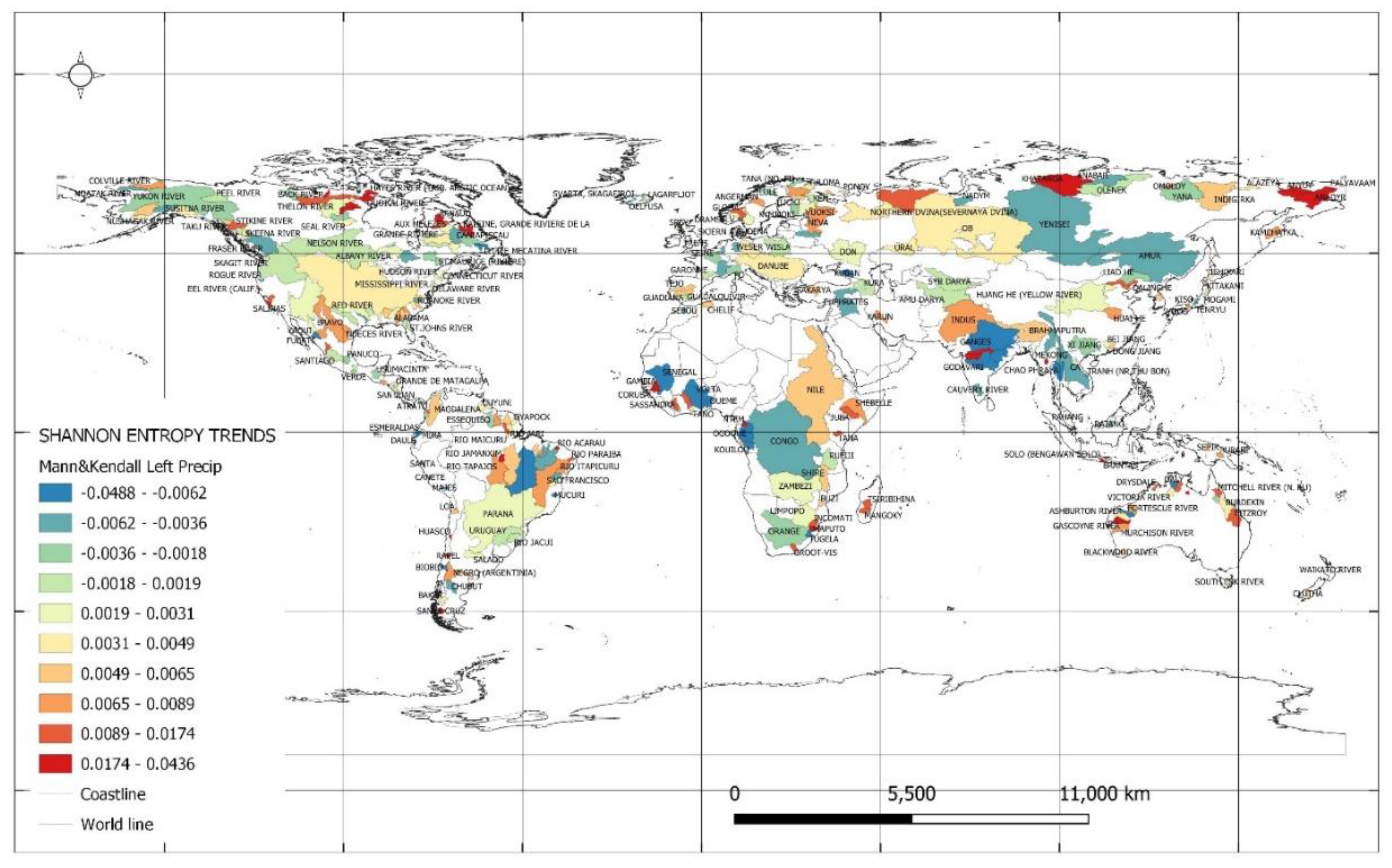
Figure 2.
Shannon entropy trends for values of maximum monthly precipitation totals.
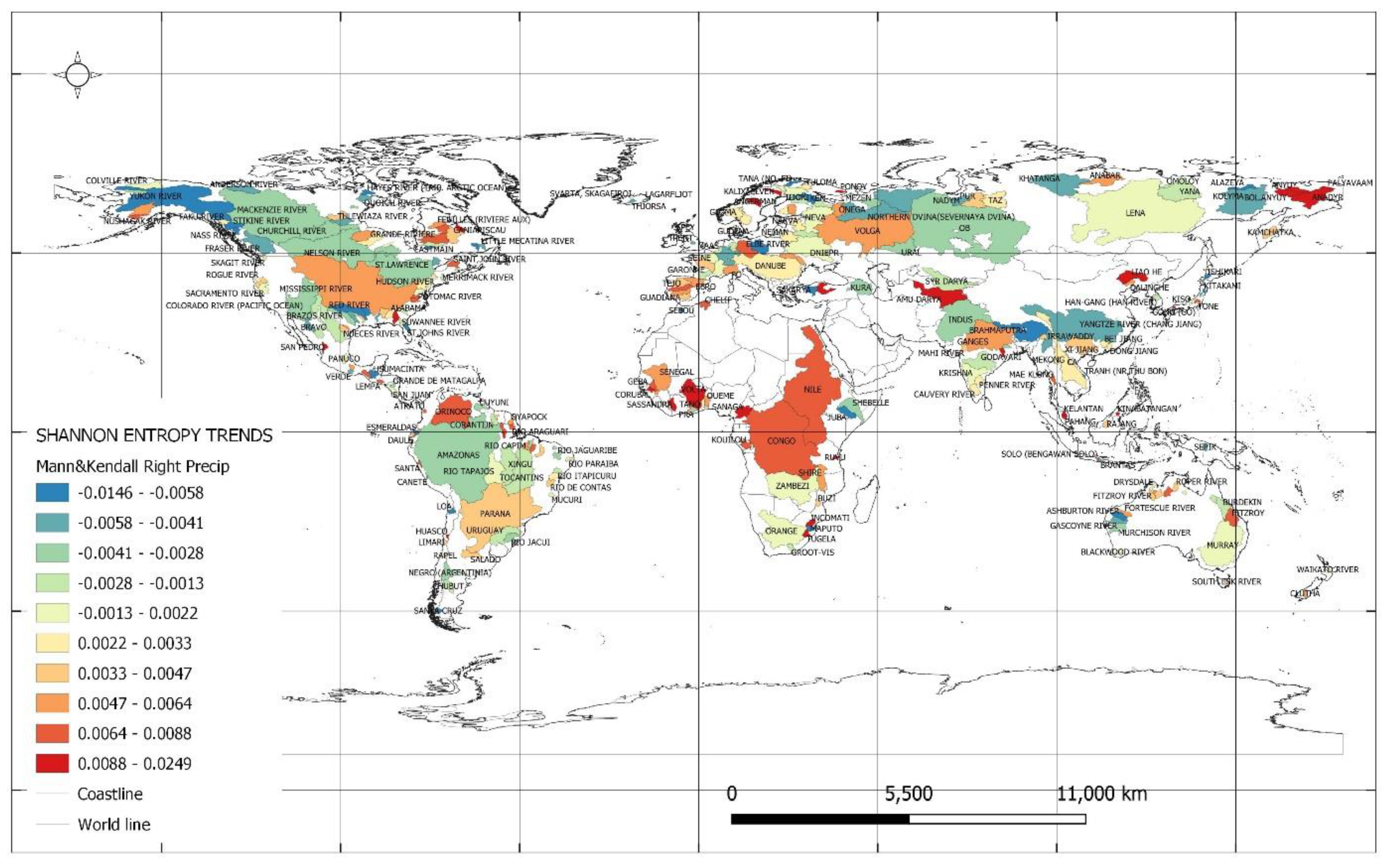
Figure 3.
Shannon entropy trends for minimum values of monthly average temperatures.

Figure 4.
Shannon entropy trends for maximum values of monthly average temperatures.
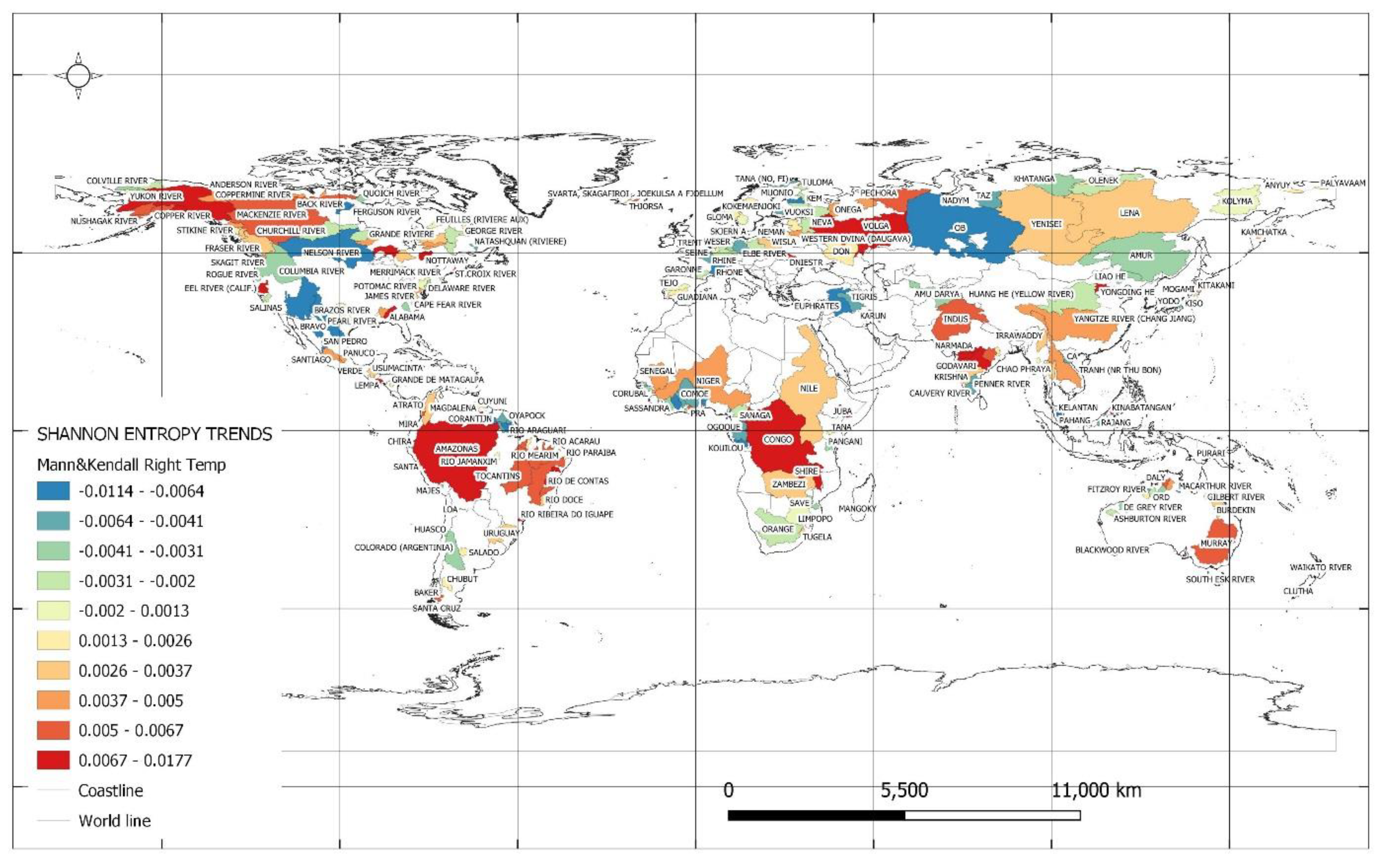
Figure 5.
Catchments in which the highest dynamics of Shannon entropy trends for minimum and maximum precipitation values were recognized at the 5% significance level.
Figure 5.
Catchments in which the highest dynamics of Shannon entropy trends for minimum and maximum precipitation values were recognized at the 5% significance level.
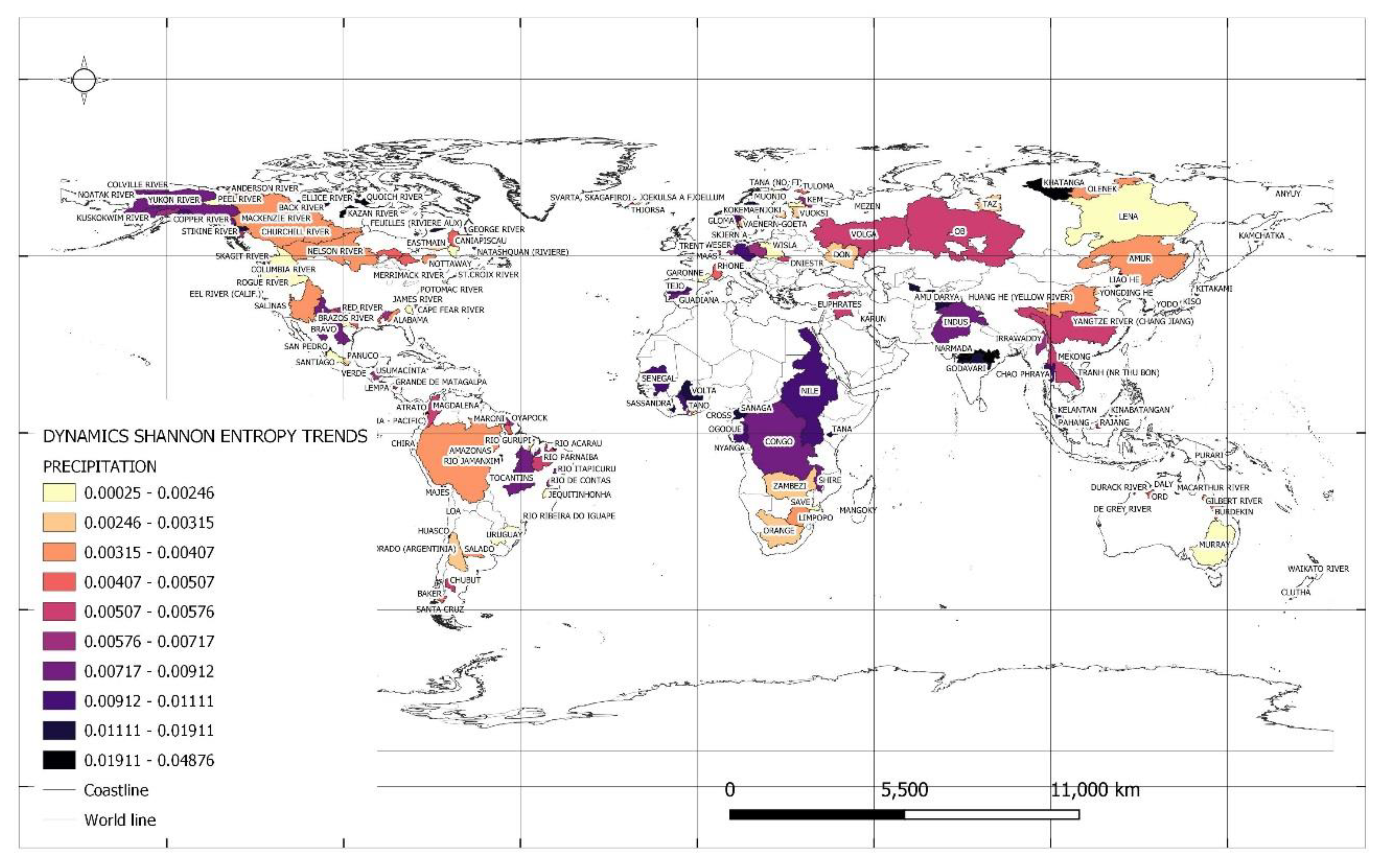
Figure 6.
Catchments in which the highest dynamics of Shannon entropy trends for minimum and maximum temperature values were recognized at the 5% significance level.
Figure 6.
Catchments in which the highest dynamics of Shannon entropy trends for minimum and maximum temperature values were recognized at the 5% significance level.
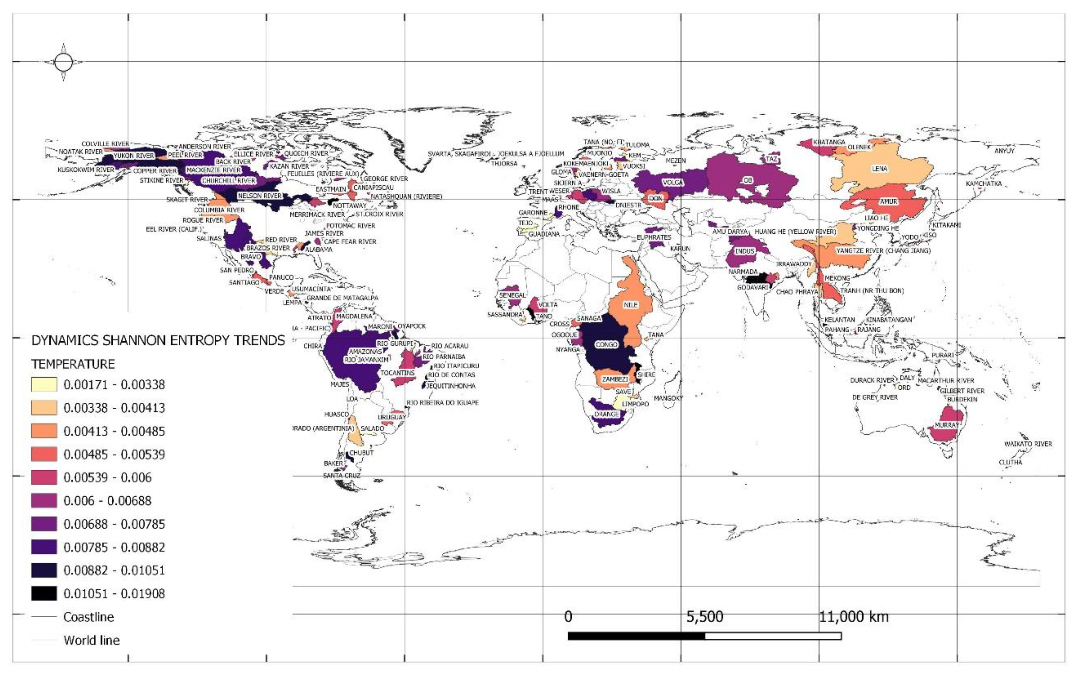
Figure 7.
Catchments in which the greatest dynamics of Shannon entropy trends for extremes of precipitation and temperature were recognized at the 5% significance level.
Figure 7.
Catchments in which the greatest dynamics of Shannon entropy trends for extremes of precipitation and temperature were recognized at the 5% significance level.
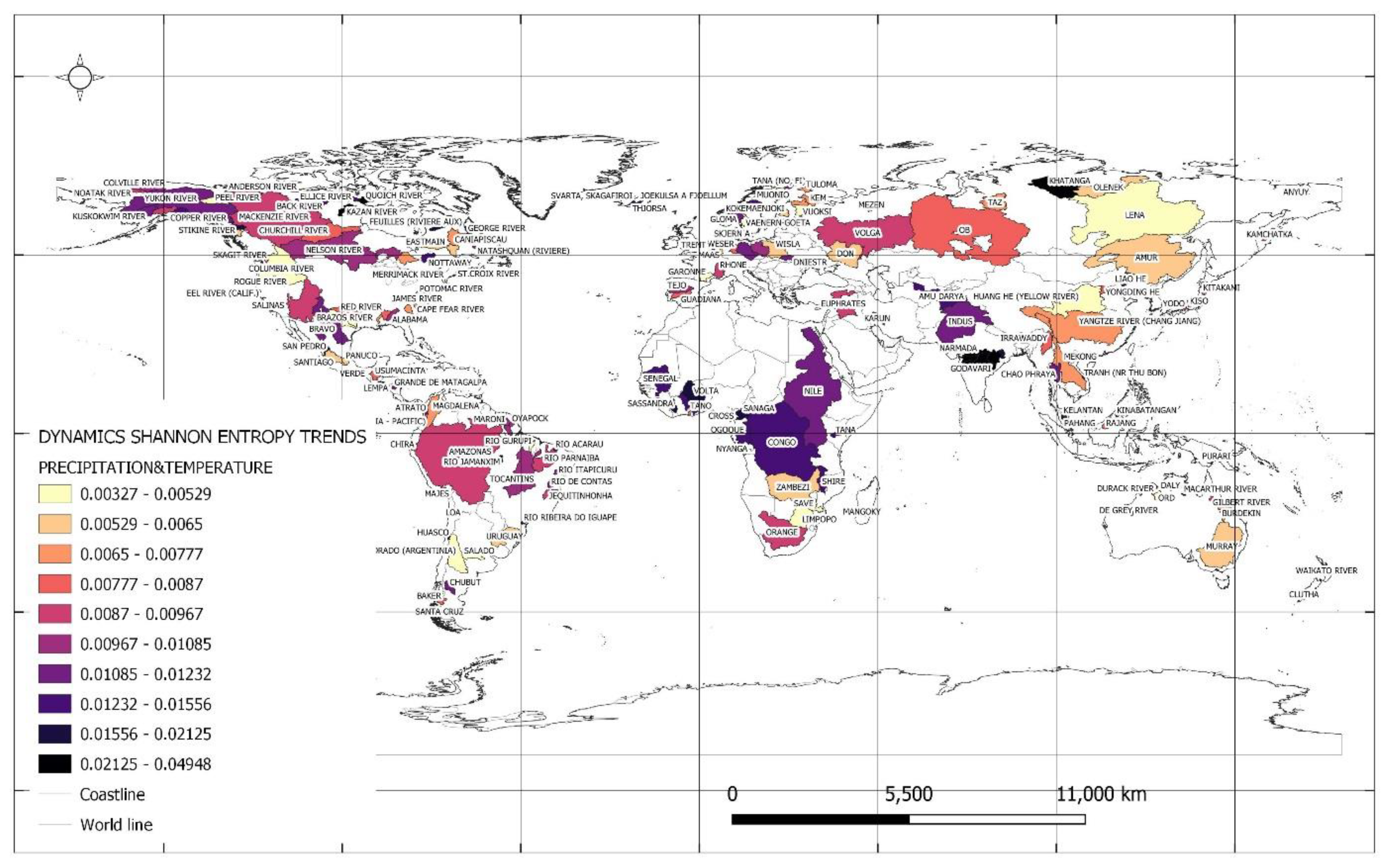

Table 1.
Areas covered in the WMO regions analysis [45].
Table 1.
Areas covered in the WMO regions analysis [45].
| Region | Continent | Lands area | Area catchment | Coverage of the continents |
|---|---|---|---|---|
| WMO | mln km2 | mln km2 | % | |
| 1 | Africa | 30.3 | 8.43 | 27.83% |
| 2 | Asia | 44.3 | 20.3 | 45.86% |
| 3 | South America | 17.8 | 12.6 | 70.57% |
| 4 | North America | 24.2 | 13.0 | 53.87% |
| 5 | Australia and Oceania | 8.5 | 1.1 | 13.07% |
| 6 | Europe | 10.5 | 6.7 | 64.10% |
| Antarctica | 13.1 | 0.0 | 0.00% | |
| Lands together | 148.7 | 65.1 | 43.77% | |
| Earth, total | 509.9 | 65.1 | 12.76% |
Table 2.
River basins in which the smallest decreasing values of Shannon entropy trends were found for minimum monthly precipitation values at the 5% level of significance.
Table 2.
River basins in which the smallest decreasing values of Shannon entropy trends were found for minimum monthly precipitation values at the 5% level of significance.
| Name of river | Name of country | Area catchment | Slope of Shannon entropy, min values | Year of change of slope of Shannon entropy min values | Slope of Shannon entropy, min values -subseries |
|---|---|---|---|---|---|
| [km2] | [bit/year] | [bit/year] | |||
| Daly | Australia | 47000 | -0.049 | 1990 | -0.025 |
| Daule | Ecuador | 8690 | -0.040 | 1988 | -0.074 |
| Mahanadi River | India | 132090 | -0.036 | 1986 | -0.006 |
| Canete | Peru | 4900 | -0.033 | 1990 | -0.017 |
| Fuerte | Mexico | 34247 | -0.026 | 1990 | -0.009 |
| Vinces | Ecuador | 4400 | -0.023 | 1990 | -0.014 |
| Little Mecatina River | Canada | 19100 | -0.017 | 1989 | |
| Kouilou | Congo | 55010 | -0.015 | 1984 | |
| Biobio | Chile | 24029 | -0.014 | 1989 | -0.012 |
| Esmeraldas | Ecuador | 18800 | -0.014 | 1991 | -0.010 |
Table 3.
River catchments in which the largest increasing values of Shannon entropy trends were found for minimum monthly precipitation values at the 5% level of significance.
Table 3.
River catchments in which the largest increasing values of Shannon entropy trends were found for minimum monthly precipitation values at the 5% level of significance.
| Name of river | Name of country | Area catchment | Slope of Shannon entropy, min values | Year of change of slope of Shannon entropy min values | Slope of Shannon entropy, min values -subseries |
|---|---|---|---|---|---|
| [km2] | [bit/year] | [bit/year] | |||
| Sittang River | Myanmar | 14660 | 0.044 | 1990 | 0.031 |
| Quoich River | Canada | 30100 | 0.040 | 1990 | 0.016 |
| Macarthur River | Australia | 10400 | 0.039 | 1990 | 0.032 |
| Bol. Anyuy | Russian Feder. | 49600 | 0.038 | 1990 | 0.011 |
| Ellice River | Canada | 16900 | 0.037 | 1989 | 0.019 |
| Anyuy | Russian Feder. | 30000 | 0.036 | 1990 | 0.008 |
| Baleine, Grande River | Canada | 29800 | 0.035 | 1990 | 0.014 |
| Khatanga | Russian Feder. | 275000 | 0.033 | 1990 | -0.002 |
| Tapti River | India | 61575 | 0.030 | 1991 | 0.006 |
| Narmada | India | 89345 | 0.029 | 1992 | 0.001 |
| Ferguson River | Canada | 12400 | 0.029 | 1990 | 0.031 |
Table 4.
River basins in which the smallest decreasing values of Shannon entropy trends were found for maximum monthly precipitation values at the 5% level of significance.
Table 4.
River basins in which the smallest decreasing values of Shannon entropy trends were found for maximum monthly precipitation values at the 5% level of significance.
| Name of river | Name of country | Area catchment | Slope of Shannon entropy, max values | Year of change of slope of Shannon entropy max values | Slope of Shannon entropy, max values -subseries |
|---|---|---|---|---|---|
| [km2] | [bit/year] | [bit/year] | |||
| Sakarya | Turkey | 55322 | -0.015 | 1987 | -0.025 |
| Stikine River | United States | 51593 | -0.014 | 1987 | |
| Brahmaputra | Bangladesh | 636130 | -0.010 | 1988 | -0.005 |
| St. Johns River | United States | 22921 | -0.010 | 1994 | -0.020 |
| Juba | Somalia | 179520 | -0.009 | 1994 | -0.004 |
| Loa | Chile | 33570 | -0.009 | 1990 | |
| Tana (No, Fi) | Norway | 14165 | -0.009 | 1992 | -0.013 |
| Ashburton River | Australia | 70200 | -0.008 | 1995 | |
| Tranh (Nr Thu Bon) | Viet Nam | 9153 | -0.008 | 1994 | -0.020 |
| Santa Cruz | Argentina | 15550 | -0.008 | 1997 | -0.022 |
Table 5.
River catchments in which the largest increasing values of Shannon entropy trends were found for monthly precipitation maxima at the 5% significance level.
Table 5.
River catchments in which the largest increasing values of Shannon entropy trends were found for monthly precipitation maxima at the 5% significance level.
| Name of river | Name of country | Area catchment | Slope of Shannon entropy, max values | Year of change of slope of Shannon entropy max values | Slope of Shannon entropy, max values -subseries |
|---|---|---|---|---|---|
| [km2] | [bit/year] | [bit/year] | |||
| Anyuy | Russian Feder. | 30000 | 0.025 | 1990 | 0.013 |
| Rio Maicuru | Brazil | 17072 | 0.018 | 1984 | |
| Bol. Anyuy | Russian Feder. | 49600 | 0.018 | 1990 | |
| San Pedro | Mexico | 25800 | 0.017 | 1995 | |
| Brahmani River | India | 39033 | 0.016 | 1990 | 0.017 |
| Anadyr | Russian Feder. | 156000 | 0.016 | 1990 | 0.007 |
| Sassandra | Cote D'ivoire | 62000 | 0.016 | 1990 | 0.005 |
| Kinabatangan | Malaysia | 10800 | 0.016 | 1988 | |
| Ponoy | Russian Feder. | 15200 | 0.016 | 1989 | 0.010 |
| Volta | Ghana | 394100 | 0.014 | 1990 | 0.008 |
Table 6.
River catchments in which the smallest decreasing values of Shannon entropy trends were found for minimum monthly average temperatures at the 5% level of significance.
Table 6.
River catchments in which the smallest decreasing values of Shannon entropy trends were found for minimum monthly average temperatures at the 5% level of significance.
| Name of river | Name of country | Area catchment | Slope of Shannon entropy, min values | Year of change of slope of Shannon entropy min values | Slope of Shannon entropy, min values -subseries |
|---|---|---|---|---|---|
| [km2] | [bit/year] | [bit/year] | |||
| Rio Ribeira Do Igu | Brazil | 12450 | -0.012 | 1990 | |
| Chubut | Argentina | 16400 | -0.010 | 1987 | |
| Ellice River | Canada | 16900 | -0.008 | 1994 | |
| Orange | South Africa | 850530 | -0.008 | 1986 | -0.011 |
| Gilbert River | Australia | 11800 | -0.008 | 1998 | -0.010 |
| Penobscot River | United States | 19464 | -0.008 | 1991 | |
| Loa | Chile | 33570 | -0.008 | 1997 | -0.009 |
| Syr Darya | Kazakhstan | 402760 | -0.007 | 1989 | -0.009 |
| Churchill River | Canada | 287000 | -0.007 | 1987 | -0.003 |
| Mono | Benin | 21575 | -0.007 | 1987 | -0.010 |
Table 7.
River basins in which the largest increasing values of Shannon entropy trends were found for minimum monthly average temperatures at the 5% level of significance.
Table 7.
River basins in which the largest increasing values of Shannon entropy trends were found for minimum monthly average temperatures at the 5% level of significance.
| Name of river | Name of country | Area catchment | Slope of Shannon entropy, min values | Year of change of slope of Shannon entropy min values | Slope of Shannon entropy, min values -subseries |
|---|---|---|---|---|---|
| [km2] | [bit/year] | [bit/year] | |||
| Svarta, Skagafiroi | Iceland | 393 | 0.019 | 1990 | 0.006 |
| Thjorsa | Iceland | 7380 | 0.016 | 1988 | 0.005 |
| Joekulsa A Fjoellu | Iceland | 7074 | 0.016 | 1988 | |
| Lempa | El Salvador | 18176 | 0.013 | 1989 | 0.011 |
| Pra | Ghana | 22714 | 0.013 | 1987 | 0.010 |
| Thames | United Kingdo | 9948 | 0.010 | 1991 | 0.007 |
| Grande De Matagalp | Nicaragua | 14646 | 0.009 | 1990 | 0.011 |
| Comoe | Cote D'ivoire | 69900 | 0.009 | 1990 | 0.012 |
| Grisalva | Mexico | 37702 | 0.009 | 1988 | |
| Sabine River | United States | 24162 | 0.009 | 1991 | 0.007 |
Table 8.
River basins in which the smallest decreasing values of Shannon entropy trends were found for maximum monthly average temperatures at the 5% level of significance.
Table 8.
River basins in which the smallest decreasing values of Shannon entropy trends were found for maximum monthly average temperatures at the 5% level of significance.
| Name of river | Name of country | Area catchment | Slope of Shannon entropy, max values | Year of change of slope of Shannon entropy max values | Slope of Shannon entropy, max values -subseries |
|---|---|---|---|---|---|
| [km2] | [bit/year] | [bit/year] | |||
| Nadym | Russian Feder. | 48000 | -0.011 | 1991 | -0.021 |
| Loa | Chile | 33570 | -0.011 | 1983 | 0.003 |
| Ferguson River | Canada | 12400 | -0.011 | 1983 | |
| Kouilou | Congo | 55010 | -0.011 | 1986 | -0.018 |
| Pahang | Malaysia | 19000 | -0.009 | 1993 | |
| Kelantan | Malaysia | 11900 | -0.009 | 1998 | |
| Karun | Iran, Islamic | 60769 | -0.009 | 1984 | |
| San Pedro | Mexico | 25800 | -0.008 | 1987 | -0.006 |
| Nelson River | Canada | 1060000 | -0.008 | 1992 | |
| Rhone | France | 95590 | -0.008 | 1989 | -0.003 |
Table 9.
River basins in which the largest increasing values of Shannon entropy trends were found for maximum monthly average temperatures at the 5% level of significance.
Table 9.
River basins in which the largest increasing values of Shannon entropy trends were found for maximum monthly average temperatures at the 5% level of significance.
| Name of river | Name of country | Area catchment | Slope of Shannon entropy, max values | Year of change of slope of Shannon entropy max values | Slope of Shannon entropy, max values -subseries |
|---|---|---|---|---|---|
| [km2] | [bit/year] | [bit/year] | |||
| Godavari | India | 299320 | 0.018 | 1991 | 0.014 |
| Tapti River | India | 61575 | 0.014 | 1988 | 0.008 |
| Mahi River | India | 33670 | 0.013 | 1990 | 0.016 |
| Lempa | El Salvador | 18176 | 0.013 | 1990 | |
| Rio Ribeira Do Igu | Brazil | 12450 | 0.012 | 1992 | 0.012 |
| Narmada | India | 89345 | 0.011 | 1987 | |
| Sacramento River | United States | 60885.7 | 0.010 | 1991 | 0.017 |
| Juba | Somalia | 179520 | 0.010 | 1990 | 0.005 |
| Nottaway | Canada | 57500 | 0.010 | 1991 | 0.008 |
| Dniestr | Moldova, Repu | 66100 | 0.009 | 1990 | 0.014 |
Table 10.
River basins with the highest dynamics calculated from Shannon entropy trend values for minimum and maximum monthly average precipitation and minimum and maximum monthly average temperatures at the 5% significance level.
Table 10.
River basins with the highest dynamics calculated from Shannon entropy trend values for minimum and maximum monthly average precipitation and minimum and maximum monthly average temperatures at the 5% significance level.
| Name of river | Name of country | Area catchment | Dynamic of Shannon entropy of precipitation | Dynamic of Shannon entropy of temperature | Multiplicity of entropy dynamics of precipitation to temperature | Total dynamic of Shannon entropy |
|---|---|---|---|---|---|---|
| [km2] | [bit/year] | [bit/year] | [bit/year] | |||
| Daly | Australia | 47000 | 0.049 | 0.008 | 5.8 | 0.049 |
| Anyuy (Trib. Kolym | Russian Feder. | 30000 | 0.044 | 0.002 | 19.8 | 0.044 |
| Quoich River | Canada | 30100 | 0.041 | 0.007 | 5.7 | 0.041 |
| Macarthur River | Australia | 10400 | 0.039 | 0.008 | 4.8 | 0.040 |
| Ellice River | Canada | 16900 | 0.037 | 0.010 | 3.9 | 0.039 |
| Mahanadi River (Ma | India | 132090 | 0.036 | 0.006 | 6.4 | 0.037 |
| Khatanga | Russian Feder. | 275000 | 0.034 | 0.006 | 5.7 | 0.034 |
| Tapti River | India | 61575 | 0.030 | 0.015 | 2.0 | 0.033 |
| Narmada | India | 89345 | 0.029 | 0.011 | 2.7 | 0.031 |
| Santa Cruz | Argentina | 15550 | 0.026 | 0.007 | 3.8 | 0.027 |
Disclaimer/Publisher’s Note: The statements, opinions and data contained in all publications are solely those of the individual author(s) and contributor(s) and not of MDPI and/or the editor(s). MDPI and/or the editor(s) disclaim responsibility for any injury to people or property resulting from any ideas, methods, instructions or products referred to in the content. |
© 2023 by the authors. Licensee MDPI, Basel, Switzerland. This article is an open access article distributed under the terms and conditions of the Creative Commons Attribution (CC BY) license (http://creativecommons.org/licenses/by/4.0/).
Copyright: This open access article is published under a Creative Commons CC BY 4.0 license, which permit the free download, distribution, and reuse, provided that the author and preprint are cited in any reuse.


