
Submitted:
25 August 2023
Posted:
29 August 2023
You are already at the latest version
Abstract
This article presents an analysis of monthly precipitation totals based on the Global Precipitation Climatology Centre database and monthly mean temperatures based on National Oceanic and Atmospheric Administration data for 377 catchments located around the world. Data sequences covering 110 years from 1901 to 2010 were analysed. The long-term sequences of precipitation and temperature were used to assess the variability of climate extremes, referred to here as polarisation. Measures of polarisation used in the natural sciences are discussed. A simple measure of polarisation was presented and applied to long-term sequences of monthly precipitation totals and monthly mean temperatures. Due to the nature of the proposed polarisation measure, other characteristics of precipitation and temperature sequences are also presented as a background for the discussion of the polarisation index. The study showed the existence of trends related to the polarisation of temperature and precipitation phenomena. As a result of the analysis, trends of polarisation factors in the area of precipitation and temperature were identified in 11 catchments out of the 377 analysed catchments. The trend analysis used Mann-Kendall tests at a level of significance of 5%. The Pettitt test was used to determine the point of trend change for precipitation and temperature data. The whole investigation is supported by rich graphical analyses, and the results are presented in tabular form.
Keywords:
polarisation of climatic phenomena
; GPCC data
; NOAA data
; monthly precipitation
; average temperature
; climate trends
; Mann Kendall test
; Pettitt test
1. Introduction
Analyses of historical observations of climate variables clearly indicate the anthropogenic causes of climate change [1,2,3]. Numerous studies at various spatial and temporal scales have thoroughly explored the impact of projected changes in the climate system on hydrology and water resources [1,3,4,5,6]. After air temperature, fresh water is proving to be the second most reactive environmental variable to climate change [1,7,8,9,10]. Despite the numerous existing studies and analyses of the temporal and spatial characteristics of precipitation and temperature, the timeliness of these studies is becoming increasingly appreciated [11,12,13,14,15,16,17,18], especially in the context of documenting the impact of human activities on regional climate factors [19,20,21]. Increasing computational capabilities and comprehensive analyses based on long measurement series [8,22,23] are attracting attention, especially in the context of the search for the justification of theses on the polarisation of extreme climatic events [1,24,25,26,27,28,29,30].
The polarisation of climatic elements is a phenomenon in which certain climatic elements or features tend to separate into two extreme or opposite categories [31,32]. This means that over time, certain climatic features become more clearly concentrated in the two opposite extremes, which can lead to increased variability and diversity in atmospheric conditions. Polarisation can manifest itself as a clear separation between extremes of temperature, precipitation or other climatic parameters, with implications for long-term patterns and trends in the climate of an area. The property of bimodality emphasises the concentration of features in two opposite extremes [8,33,34,35]. The polarisation of precipitation events can be defined as a process in which the frequency and intensity of extreme precipitation events, such as rainstorms, hail, storms or floods, increases. Simultaneously, the "normal" precipitation condition is becoming less frequent. In the case of temperature phenomena, polarisation can be defined as a process in which the frequency and intensity of extreme temperatures, such as heat waves or extreme cold, increases. Again, the "normal" state of temperatures is becoming increasingly rare. Both of these phenomena are part of a broader process of climate change that affects atmospheric circulation and processes, leading to increased weather variability and a greater risk of extreme weather. Polarisation can be interpreted as a change in the nature of the occurrence of extreme events, where extreme events, specifically extreme temperatures and precipitation, are becoming more frequent, while "normal" conditions are becoming less frequent.
The increased interest in climatic factors such as precipitation and temperature [13,36,37] is also due to the consequences of floods and periods of hydrological drought [38]. Studies of the variability of precipitation and temperature over different periods [5,9,14,39,40,41] have made it possible to analyse statistical trends and assess the signal of these changes [37,42,43,44]. The results of these analyses provide information about the moments of trend change and the form of them. In the context of the importance of the variability of climatic factors, it is important to apply statistical techniques [4,45] that allow the detection of changes and trends [2,43], in among other sources, data relating to monthly precipitation totals and monthly average temperatures.
Climate change predicted by the IPCC (Intergovernmental Panel on Climate Change) occurs as a result of increases in greenhouse gas emissions, which are mainly caused by the industrialisation of the world, the burning of fossil fuels and changes in land use [3,10,46,47]. According to the Intergovernmental Panel on Climate Change [48], both natural forces and human activities contribute to changes in climate patterns, including increases in land and ocean surface temperatures, changes in spatial and temporal precipitation patterns, increases in the frequency of extreme events, rising sea levels and increased El Niño [3,4,36,39]. It is clearly emphasised that human influence significantly outweighs the action of natural forces. The warming of the Earth is evident in data that show a 0.6°C increase in global temperature from 1901 to 2001 [48]. To see changes in precipitation and temperature trends, anomalous values and statistical models are used to measure the timing of the trend change and its magnitude. The change in trends of various climate variables can be quantified using global atmospheric circulation models (GCMs) or, for example, using statistical models that identify the moment of change of the trend and its magnitude [8].
Many studies have shown that climatic variability has a significant impact on river flow values, which are sensitive to both precipitation and temperature. The polarisation of climatic phenomena has been demonstrated by researchers [40], who found increasing trends mainly in flood magnitude in German river catchments, which was attributed to climate change. In addition, seasonal analyses have shown that these changes were greater in winter than in summer. Rapid changes in both mean and variance can be attributed to both climate (e.g., changes in climate regimes) and anthropogenic effects (e.g., construction of dams and reservoir systems, changes in land use and vegetation cover, changes in the location of measurement points) [49,50]. Statistical analyses must be interpreted in the context of observed physical [3,7,51], social and economic phenomena [3,14,19,52]. Therefore, predicting temporal trends in precipitation and temperature is very useful in social and urban planning [53].
The world's rivers play a key role in linking the atmosphere, hydrosphere and biosphere by transporting 40% of precipitation runoff and 95% of sediment to the oceans [54,55]. The shaping of river flow depends on many factors, such as precipitation, temperature, evaporation, soil conditions, landforms and land use changes [56]. With the available long-term precipitation and temperature data, it is very important to conduct long-term analyses of this data in order to understand the polarisation of climate phenomena and its potential consequences [57]. In addition, such analyses provide valuable information that can be used to develop decision-making tools for the purposes of effectively managing extreme events, such as droughts and floods, and to mitigate ecological damage in regions particularly vulnerable to these hazards [57].
When assessing climate polarisation, a process in which certain climatic features become concentrated in two opposing categories, there are strong links between precipitation and temperature [39,57,58]. An increase in global temperatures can lead to an increase in the amount of water vapour in the atmosphere. More water vapour in the atmosphere increases the potential for cloud formation and precipitation, especially in areas with higher temperatures where there is access to more thermal energy As a result, more water vapour may in turn increase precipitation, meaning that areas with higher temperatures may experience more precipitation. Conversely, lower temperatures can result in reduced precipitation. In extreme cases, such as prolonged droughts or floods, fluctuations in temperature and precipitation can have catastrophic consequences, including the failure of crops and damage to property [1,50,59].
Long-term data series make it possible to identify temperature and precipitation trends and help to determine whether a region is experiencing changes in polarity. Furthermore, the analysis of precipitation-temperature interactions provides a better link between important atmospheric phenomena, such as El Niño and La Niña cycles [60,61], which affect global climate patterns. An example of this is the fact that rising temperatures can affect the occurrence of intense precipitation, while reduced precipitation can contribute to extreme heat waves [50]. It is import to consider the amount of precipitation and temperature along with other climate phenomena as their interaction can affect the overall effect of climate polarisation [62]. Understanding magnitudes and the relationship between precipitation and temperature is crucial for assessing the polarisation of climate phenomena and its consequences for the environment, economy and society. This knowledge is essential with regard to taking preventive measures in order to mitigate the negative effects of climate change.
The main topic of this study is the analysis of long-term sequences of precipitation and temperature data in terms of the possibility of introducing the concept of polarisation of climate extremes. Section one reviews the literature and presents the background of the variability of extreme climate events that provide the basis for analysing the polarisation phenomenon. Section two presents the temporal and spatial extent of the data that was used in the analysis. Section three characterizes the phenomenon of the polarisation of extreme climate events in the areas of precipitation and temperature, and discusses the impact of polarisation on important consequences for ecosystems, economies and infrastructure. The fourth section presents the approaches used in constructing a measure of polarisation and presents a proposal for the introduction of a static measure based on a stationary time series and a dynamic time series based on trends. The fifth and sixth sections present known statistical techniques in trend analysis and trend change point recognition. The seventh section discusses and evaluates the results of the performed analyses. The eighth section presents conclusions.
2. Preparation of Data for Analysis
The great interest in analysing long precipitation sequences stems from the need to assess climate change and its impacts on all spatial and temporal scales. This demand has led to the initiation and support of many research and monitoring programs conducted by international organisations. In this context, the Global Precipitation Climatology Centre (GPCC) was established on behalf of the World Meteorological Organization (WMO) in 1989. This institution is supported and operated by the Deutscher Wetterdienst (DWD, Germany's National Meteorological Service) as a German contribution to the World Climate Research Program (WCRP). The main objective of the GPCC is the global analysis of monthly precipitation on the Earth's surface based on "in situ" precipitation station data [36,63]. An equally important institution is the NOAA (National Oceanic and Atmospheric Administration) the US government agency for the study of the atmosphere, oceans and climate. It conducts research and monitoring of climate change, including collecting, processing, analysing, updating and making long-term precipitation and temperature sequences available [64,65].
The goal of the aforementioned institutions is to meet user requirements for the accuracy of the data and analysis results made available, as well as the timelines and availability of the product. Among the various types of GPCC and NOAA products, gridded sets of long-term precipitation and temperature data are made available [63,64]. These items of data are not made available in real time. This paper relies on grid data of monthly precipitation totals from the GPCC products made available and grid data of monthly mean temperatures from NOAA products. This data corresponds to a spatial resolution of 0.5°x 0.5°, are consistent in spatial and temporal extent and cover the years 1901 to 2010. Products from both the GPCCC and NOAA are made available via the Internet.
The NOAA (National Oceanic and Atmospheric Administration) and the GPCC (Global Precipitation Climatology Centre) are two institutions that provide the opportunity, based on the available long-term data, to perform analysis and evaluation of the polarisation of climatic phenomena. The NOAA is engaged in the research and monitoring of the atmosphere, oceans and climate around the world. The NOAA collects data from various sources such as satellites, ocean buoys, aircraft and weather stations to assess the state of the climate and predict changes. The GPCC is involved in assessing precipitation around the world. The GPCC uses a variety of data sources, such as weather stations, radar and satellites, to develop global precipitation maps. The two institutions use their knowledge and data to assess changes in climate phenomena, including precipitation and temperatures around the world, and predict how they will change in the future. They are also working with other climate institutions to increase understanding of the climate and to help make decisions about climate change. This paper examines global trends in monthly precipitation totals and monthly mean temperatures from the area of 377 river basins distributed over all of the continents. Assuming 509.9 106 square kilometres of land area on the earth, the analysis covers 12.76% of the total land area of the globe. Table 1 shows the areas covered by the analysis. The regions in the text are identified by code where (Table 1, Figure 1).
GPCC precipitation data and NOAA temperature data by month from 1901 to 2010, calculated from grid data with a spatial resolution of 0.5°x 0.5° ° latitude and longitude, were converted to catchment areas. In this way, a sequence of monthly data was obtained, which became the subject of the analyses presented in this article. GIS interpolation mechanisms were used in the spatial analysis of the data preparation. The monthly precipitation amount and the monthly temperature value were calculated as a weighted average of the corresponding features of the grid surface elements that completely covered the catchment area, taking into account the surface area of these elements.
The area of one of the smallest catchments in this study: SKJERN A (Europe, Denmark) is, according to calculations, 1090 km2. An area of 0.5°x 0.5° at the latitude of Denmark covers an area of 3100 km2. The location of this catchment area, for calculations of precipitation or temperature, requires the consideration of five neighbouring areas of 0.5°x 0.5°. With even such a small catchment area, precipitation and temperature characteristics are averaged. The calculated values of the sequences were subjected to a simple statistical analysis, determining the basic statistics: the minimum and maximum value, the mean and, the standard deviation of the sample. The data was analysed in monthly as well as calendar year cross sections. Analyses of temperature data covered the years 1901 to 2010.
4. The polarisation of precipitation and temperature phenomena
The occurrence of temporal variability and extreme events in air temperature and precipitation is usually assessed by analysing a set of indicators that define variability and extreme conditions. The common understanding of an extreme event is based on the assumption that a "normal" condition exists [44]. In the context of the common understanding of an extreme event, polarisation can be interpreted as a change in the nature of the occurrence of extremes, with extreme events – extreme temperatures and precipitation – becoming more frequent and the "normal" state becoming less frequent. The polarisation of extreme events can result from a variety of factors, including human activity and climate change, which can affect precipitation cycles, the intensity of extreme events and temperature conditions. In this way, polarisation can be interpreted as the evolution of climatic features, resulting in an increase in the frequency of extreme events while destabilising the 'typical' state. Polarisation can have serious consequences for the functioning of ecosystems, the economy and the quality of human life.
Analysis of the polarisation of precipitation and temperature is essential because of their key role in global energy and water cycles and their impact on climate change. Accurate knowledge of precipitation and temperature is particularly important for assessing the amount of available freshwater and managing water resources, which is essential for reducing the risk of floods and droughts. In addition, there is growing scientific evidence that human activities are influencing climate change, contributing to shorter periods of intense precipitation and longer dry periods of high temperature and low precipitation. The polarisation of extreme events, such as floods and droughts, is increasingly evident and can be attributed to the unevenness and intensity of human activity. Investigating the polarisation factors associated with monthly precipitation and monthly average temperatures can significantly influence the development of water management strategies and reduce the risk of extreme climatic events.
This article analyses long-term sequences of precipitation and temperature to assess the polarisation of climate phenomena. The term "polarisation" in terms of precipitation or temperature is used in climate science to describe the process by which some areas of the planet become more extreme in terms of temperature and/or precipitation. This can lead to significant changes in the local environment, including changes in the distribution of plant and animal species, changes in weather patterns and changes in sea level [66]. Long-term sequences of precipitation and temperature are an essential tool for studying climate polarisation. These sequences provide a detailed record of an area's climate over many years, allowing trends and patterns in the data to be identified. By analysing these sequences, it is possible to identify areas where the climate is becoming increasingly polarized and track changes over time. One of the key advantages of using long-term precipitation and temperature sequences is that they provide a high degree of accuracy and precision. The time series are created using advanced measurement techniques, such as data from satellites and weather stations, and are subject to rigorous quality control measures [27,63,67]. As a result, they provide a reliable record of climate data in a given area, enabling precise observations and measurements.
The impact of polarisation can be observed in various areas of life on earth: in ecosystems, the economy and infrastructure, in changes in the size and location of water resources. The impact of polarisation on ecosystems in areas of extreme temperature and precipitation changes affects biodiversity and ecosystem functioning [66]. The polarisation of climatic factors can lead to changes in the distribution of plant and animal species [68,69], which can have negative consequences for entire ecosystems. The consequences of polarisation for agriculture can affect crops and food production [17,41]. In some regions, climate polarisation may lead to a reduction in the amount of available water resources, which in turn affects agricultural production and the health of the industry. The consequences of polarisation for infrastructure can affect roads, bridges, buildings, water and sewage networks and water management systems. In extreme cases, severe damage or destruction can occur. Due to the complex and dynamic nature of the climate [70,71], polarisation is variable and difficult to predict. It is also difficult to predict exactly what the consequences of polarisation will be in a given region. In addition, climate variability means that some regions may experience polarisation in different years, complicating the process of predicting and monitoring changes. The interaction between polarisation and other climate phenomena can trigger certain climatic events, such as hurricanes, tornadoes or droughts. In this way, one phenomenon can amplify or weaken another, complicating the process of understanding the scale of climate change. The influence of anthropogenic factors on the polarisation of climate factors can occur through greenhouse gas emissions [17,47,57,62], among other factors.
Polarisation of climate events refers to changes in the intensity and frequency of influential weather events. NOAA and the GPCC monitor these changes [63,72] to determine the factors influencing the polarisation of climate phenomena, their effects, and ways to reduce the negative consequences associated with these events. Assessing temperature variability is crucial to understanding climate change and its impact on ecosystems and people [73]. All of this information is essential for developing strategies and actions to manage change and to adapt and minimise its negative impacts. NOAA and GPCC are key sources of information for scientists, policymakers and other stakeholders who make decisions about climate change.
5. The concept of polarisation measure
The concept of measuring climate polarisation is based on measuring the degree of diversity and variability of climate elements in a given area. This measure is used to determine the level of polarisation of climate elements in the region of interest. Polarisation refers to the extremes of parameters such as temperature, precipitation, humidity, etc. occurring in a specific area. A high level of polarisation indicates significant differences between maximum and minimum values, which can lead to an increased risk of extreme weather events. The measure of polarisation can be determined from various climatic parameters, such as temperature, precipitation, humidity and atmospheric pressure. This can be calculated on different spatial and temporal scales, for example, for the entire country over the course of a year, for a specific region over the course of a month, or for individual weather stations over the course of a day. Depending on the purpose of the study and the availability of data, the measure of polarisation can be determined for different combinations of parameters. It is worth noting that a high level of polarisation does not necessarily mean unfavourable climatic conditions. For example, some regions have significant temperature differences between summer and winter, which can have a positive impact on seasonal tourism. However, in other cases, high polarisation can lead to serious problems, such as droughts, floods or storms. Therefore, a measure of polarisation can be useful in identifying areas that require special attention when planning climate change adaptation activities.
Different approaches are possible for constructing measures of polarisation in climate phenomena, depending on the type and scale of the data under analysis. One of the basic methods is to use probabilistic techniques based on classical theories of one- or multi-dimensional random variables with distributions built using Copula functions [53,74,75]. Other, simpler methods are based on statistical characteristics [4,10,33,45]. A simple concept is to construct indicators measuring the degree of extremity that a phenomenon can take, for example, by measuring the dispersion relative to the long-term average. An example of such an indicator is the coefficient of variation. Another way to create a polarisation indicator is to define it as the degree of extremity compared to the mean value relative to the variability measured by the dispersion measure [12,76,77]. Such indicators can be based on classical measures, such as variance, standard deviation, mean deviation and the coefficient of variation, or on positional measures, such as range, quartile deviation and the coefficient of variation [33].
Further methods of building indicators are based on the idea of unevenness [78,79], which can also be a measure of polarisation. One such indicator is kurtosis [80], which is influenced by the intensity of extreme values, so it measures what is happening in the "tails" of the distribution. Other types of indicators are measures that have their genesis in economics and econometrics. One such example is the Gini index, also called the Gini coefficient [77,81,82,83,84], built using the Lorentz curve, which describes the degree of concentration of a one-dimensional distribution of a random variable with non-negative values [82]. The Gini index ranges from a minimum value of zero, when all values are equal, to a theoretical maximum of one in an infinite population in which every element except one has a magnitude of zero. In the context of climate change, the Gini index can be used to measure inequality in exposure to the effects of climate change, such as droughts, floods or sea level rises [62]. Higher values of the Gini index indicate greater inequality in the occurrence of these phenomena. Several other examples of measures can be cited, including the following:
- The concentration ratio [85] determines the degree of concentration of values at one end of the distribution and is similar to the Gini coefficient. However, it should be noted that the Gini coefficient may be less useful in analysing asymmetric distributions, which means that other indicators such as the concentration ratio or Lorenz curve should be considered in such cases.
- The GMD (Gini Mean Difference) index [86] is an inequality measure used in statistical and econometric analysis to measure polarisation or inequality in a sample distribution. Unlike the Gini coefficient, which measures unevenness, the GMD index enables the analysis of unevenness in the distribution of any variable, such as income, age, weight, height, precipitation and temperature. The GMD index ranges from zero to one, where zero indicates complete evenness in the distribution and one indicates the concentration of all values in one class. The higher the GMD index value, the greater the unevenness in the variable distribution.
- The Lorenz indicator [78,82] is an inequality indicator in a distribution, which is based on the Lorenz curve. It is often used to measure income inequality but can also be used to measure inequality in other quantitative variables, including climate change studies. Higher values of the Lorenz curve indicate greater inequality in the occurrence of climate change effects such as droughts, floods, or sea level rises, meaning that some regions or social groups are more vulnerable to the effects of climate change than others.
- The Atkinson index [77] is a measure of inequality in the distribution of quantitative variables, which is based on the idea of absolute deviations. It takes into account the differences between groups of values in the distribution; it is similar to the Gini index, but focuses more on average values than extreme values.
- Range relates to values calculated as max-min usually refering to the difference between the maximum and minimum values of a given variable in a specific period of time. In the case of assessing the polarisation of precipitation and temperature, max-min can be used as a measure of the amplitude of these variables in a given period.
In this study, two measures are adopted to evaluate the phenomenon of polarisation, the first is built based on a stationary time series, the second is based on calculated trends.
The first measure is defined as follows:
where:
- the amplitude of change, range, the evaluated changes or ranges are taken over a selected period of time (110 years), the difference between the maximum and minimum value of a characteristic - is a measure that characterizes the empirical area of variation of the studied characteristic;
- standard deviation.
The amplitude of change values can be useful in identifying extreme climate conditions, such as periods of drought or heat waves, as well as periods of intense precipitation or extremely low temperatures. However, max-min as a single measure may be limited in its usefulness because it does not take into account other factors such as the length and intensity of the period, as well as other variables that affect weather conditions. Due to the fact that it ignores all data except for two extreme values, it does not provide information about the diversity of individual feature values in the population. Therefore, along with max-min values, other measures such as mean values, standard deviations, or cumulative indices are typically used to obtain a more comprehensive and diverse view of climate variability. For example, max-min values can be calculated for individual months, seasons or years, and then compared with mean values, standard deviations, or other measures to better describe climate variability over time and space.
The adopted measure, which is the ratio of the max-min values to the standard deviation , can be used as a measure to evaluate the polarisation of precipitation and temperature. The values refer to the amplitude of changes of a given variable over a period of time, while the standard deviation σ refers to the degree of variability of these values around their mean. By applying this measure, we can see how large the amplitude of changes is in relation to the variability around the mean. Values of this measure greater than 1 suggest that the amplitude of changes is greater than the variability around the mean. If the variability is relatively low compared to the amplitude, it may indicate the occurrence of periods of extreme climatic conditions, such as periods of drought or heatwaves, as well as periods of intense rainfall or extremely low temperature. However, the use of a single measure may be limited because it does not take into account other factors affecting climate variability. Therefore, it is worth using it together with other measures that show the character of climate variability. Note that the values of this measure for precipitation and temperature will always take a non-negative value.
The second form of adopted measures could be dynamic indicators showing the variability of the indicator over a longer period of time. The simplest indicators are based on the idea of a trend coefficient. Trend is a long-term feature referring to the general direction of changes over time in the value of a variable. Trend can indicate an increase, decrease, or stabilization of the variable over time. In time series analysis, the trend coefficient is one of the basic elements that help to forecast future values of the variable. The trend can be analysed for different time scales, from short-term cycles to long-term trends [2]. Trend analysis is applied in many fields, such as economics, finance, meteorology, earth sciences, medicine, sociology, and marketing. In scientific research, trend analysis is often used to study changes in long-term time series, such as climate change, demographic changes, or evolution of species.
The second measure is defined as:
where
is the trend of the amplitude of changes, range or difference between the maximum and minimum value of the variable - it is a measure characterizing the empirical range of variability of the studied feature;
is the standard deviation to be evaluated are taken over a selected period of time (110 years).
The above measure can be interpreted as the ratio of the trend in variability of the amplitude to the trend in variability of the standard deviation. The trend in variability of the amplitude refers to the direction and speed of changes in the maximum and minimum values of a given variable over time, while the trend in variability of the standard deviation refers to the direction and speed of changes in the variability of the values of a given variable around their mean over time. Values of this measure greater than 1 suggest that the trend in the increase of amplitude changes is stronger than the trend in the increase of variability around the mean. This means that changes in the maximum and minimum values of a given variable are increasing faster than the variability around their mean, which may indicate the occurrence of extreme weather conditions. In the proposed measure, the trend of the ratio of the indicators was not calculated, but the trend of the numerator and denominator was separately maintained. Both measures are used to assess trends in data, but they differ in how they relate to data variability.
The measure: was not used because max-min changes are normalised by the standard deviation, meaning that high data changes in one direction can be offset by changes in the other direction.
The measure , by contrast, uses two indicators of data variability: trend amplitude and trend standard deviation. The use of amplitude in this formula means that more emphasis is placed on the extreme values of the data, rather than its overall variability. Therefore, when one is interested in more extreme values in the data, the measure adopted may be a better choice.
Note that the values of this measure for precipitation and temperature can be negative as well as positive. In the case of negative values, this means that the trends of polarisation factors (amplitude and variability) will be opposite, in the case of a positive value, the trends of polarisation factors will be consistent.
6. Detecting a change point in the trend
Various methods can be applied to determine change points in a time series [88], [8,89,90,91]. In this analysis, the non-parametric Pettitt change point test (PCPT) [92] was used to detect the occurrence of changes. The Pettitt test (PCPT) is a non-parametric test for detecting sudden changes in a time sequence. It is used to detect the turning point where a sudden change, known as a "jump", occurs in the time series. The Pettitt test (PCPT ) involves comparing the sum of ranks of two subsets of data, which are divided by a threshold value, to determine whether there is a statistically significant change in the time sequence.
This test can be applied to analyse data with any distribution, and the test result is not dependent on the data having a normal distribution. The result of the Pettitt test (PCPT ) is a test statistic value, which is compared with the critical value for the level of significance to determine whether the null hypothesis of no sudden changes in the time sequence can be rejected. The rank is given after sorting and is dependent on the variable that gives the order of the records in the set.
The PCPT has been widely used to detect changes in observed climatic and hydrological time series [8,16,93,94]. The Pettitt test is also applicable to investigate an unknown change point by considering a sequence of random variables , which have a change point at . As a result has a common distribution , but have a different distribution , where . The null hypothesis : no change (but ); is tested against the alternative hypothesis : change (lub ); using the non-parametric statistic where:
for the downward shift and or the upward shift [91]. The confidence level associated with lub is approximately determined by:
When is smaller than the specified confidence level (for example, in this study, 0.95 was adopted), the null hypothesis is rejected. The approximate probability of significance for the change point is defined as:
It is obvious that in the case of a significant change point, the series is segmented at the change point into two sub-time series.
The main aim of this study is to investigate the existence of change points in the time series of monthly sum precipitation and monthly average temperature characteristics. For time series showing a significant change point, the trend test is applied to partial series, and if the change point is not significant, the trend test is applied to the entire time series [8].
7. Trend test
To examine the trend in a given time series, the Mann-Kendall test (MKT) can be applied. Originally, this test was used by Mann [95], and later Kendall in 1975 derived the distribution of the test statistic [91]. This test is independent of the type of distribution and we do not need to adopt any specific form of the data distribution function [96]. This test was widely recommended by the World Meteorological Organization for public applications, and has been used in many scientific studies to assess trends in water resource data [2,8,91]. Therefore, the MKT has been recognised as an excellent tool for trend detection by other scholars in similar applications. It should also be noted that the MKT test considers only the relative values of all elements in the series . for analysis. The test statistic for the MKT test is given by:
where are the consecutive values of the data, and n is the number of elements in the data. Under the null hypothesis of no trend, and assuming that the data are independent and identically distributed with a zero mean and a variance denoted by , which is calculated as ( - the repeated values in the analyzed sequence):
To test a hypothesis, the standard normal distribution is used, denoted as the test statistic , which is defined as follows for the trend test:
In the two-sided test for trend, the null hypothesis is represented as: : there is no trend in the dataset, which will be rejected if the calculated statistic is greater than the critical value of this statistic obtained from the standard normal distribution table corresponding to the previously established level of significance. A positive value of indicates an increasing trend, and a negative value indicates a decreasing trend.
9. Results and Discussion
In the present study, the following properties of long-term sequences of monthly precipitation totals and monthly mean temperatures were investigated for 377 catchments from the area of 6 WMO regions.
The scope of research and calculations included:
- the determination of the values of long-term monthly strings over a period of 110 years;
- the calculation of statistics relating to average values for each calendar month, the minimum value, the maximum value, the mean value and the standard deviation;
- the determination of the values of these trends with the Mann Kendall test (MKT) being used to evaluate the trend values;
- the examination of whether the long-term series showed change points using the Pettitt test (PCPT);
- the examination of whether the sub-series (after the point of change up to 2010) has a significant trend in cases in which the long-term series showed points of change and to what extent this trend has changed.
Of all the catchments analysed in terms of sequences of monthly precipitation totals, only for one catchment of the LAGARFLJOT River located in Iceland (EUROPE) was it shown that four tests (MKT for RANGE, MKT for STD, PCPT for trend change and MKT for new trend) were simultaneously satisfied. This means that at the 5% significance level for this catchment, the measure trend was recognised, the year of the trend change was determined, and additionally the new trend was recognised. The RANGE trend changed not only in value, but also in direction, from negative to positive, from a value of (-0.136) to a value of (0.310) in 1953, and the STD trend changed from a value of (-0.533) to a value of (0.889) also in 1953. In the case described for the LAGARFLJOT catchment, both the values and directions of the RANGE and STD trends changed. The change in the direction of the RANGE trend from negative to positive means that in 1953, there was an increase in the maximum value of monthly precipitation in the study area, while the STD trend indicates that the variability of this phenomenon has also changed. The main reason for these changes is the economic and demographic development in the area. In 1947, the town of Egilsstadir was founded in eastern Iceland on the banks of the Lagarfljót River and became the largest town in eastern Iceland and its main service, transport and administrative centre. It is now the largest settlement in the eastern region. In the 1950s, Iceland saw a surge in the use of oil as a heating medium. This resulted in increased CO2 emissions, rising temperatures and may have caused changes in rainfall patterns [99].
Based on the analysis of monthly precipitation data in the analysed catchments, it should be noted that for 93/377 catchments, i.e. in 25% of the analysed catchments, the trends of polarisation coefficients (RANGE and STD) in monthly precipitation totals were confirmed at the significance level of 5%, while in the remaining 75%, the trends were not confirmed.
Analysing the values (Figure 2) of the polarisation coefficient sequentially in the ten largest catchments ranging from 244,000 – 2,900,000 km2 showed (): NILE (Africa, Egypt): 4.26/0.71, YENISEI (Asia, Russian Federation): 4.25/0.64, JANGCY RIVER: 5.28/ 0.66, GANGES: 3.81/1.24, HUANG HE (Asia, China): 6.11/1.01, BRAHMAPUTRA (Asia, Bangladesh): 5.42/0.94, AMU DARYA (Asia, Uzbekistan): 5.10/0.83, EUPHRATES (Asia, Iraq): 5.93/0.84, SENEGAL (Africa, Senegal): 4.95/1.34, and URUGUAY (South America, Uruguay): 7.15/1.34. The highest value of this assumed polarisation index among the ninety-three catchments was obtained at 12.78 for the COPPER RIVER catchment (North America, United States), and the lowest was at 3.81 for the GANGES River catchment (Asia, India).
Analysing the values (Figure 3) of the trends of polarisation factors, (trend(RANGE) and trend(STD)) were shown at a significance level of 5%. The following values were obtained from the next ten largest catchments ranging from 244,000 – 2,900,000 km2, namely NILE (Africa, Egypt): 2.28, YENISEI (Asia, Russian Fed.): 3.66, YANGTZE RIVER (Asia, China): 4.69, GANGES (Asia, India): 3.20, HUANG HE (Asia, China): 4.02, BRAHMAPUTRA (Asia, Bangladesh): 5.17, AMU DARYA (Asia, Uzbekistan): 3.31, EUPHRATES (Asia, Iraq): 3.81, SENEGAL (Africa, Senegal): 3.00, and URUGUAY (South America, Uruguay): 3.55. The highest value of this assumed polarisation index, among the ninety-three catchments, was obtained at 5.17 for the BRAHMAPUTRA (Asia, Bangladesh) river catchment, the lowest was at 2.28 for the NILE (Africa, Egypt): river catchment.
Figure 4 shows the spatial location of the analysed catchments, where significant trend change points in the polarisation coefficients of monthly precipitation were recognised at the 5% significance level. For the catchments of the rivers of Africa, the years of changes in rainfall trends mainly occur in the late nineteen-sixties to the nineteen-seventies. Changes in trends can be linked to processes of decolonisation, independence and economic development in the area. The apogee of this process occurred between 1960 and 1968, and 1960 is referred to as the 'Year of African Independence' [100]. For the catchments of the rivers of Asia, the years of changes in rainfall trends mainly occur in the range of the nineteen-fifties to the nineteen-sixties in the area of Russia, the nineteen-forties to the nineteen-sixties in the area of China, and from the nineteen-thirties to the nineteen-seventies in the area of India. The 1950s in Russia saw intensive economic development, industrialisation and intensive agricultural development [101]. 1949 was the beginning in China of land reform and nationalisation of the main economic sectors. The 1970s was the Cultural Revolution where economic development collapsed [102]. For the catchment areas of South American rivers, years of changes in precipitation trends mainly occur in the period from the nineteen-forties to the nineteen-seventies. The 1960s and 1970s were a watershed period in the economic development of Latin American countries [103]. In the area of North America, this period is from the nineteen-forties to the nineteen sixties on the west coast and through the nineteen-sixties for the east coast. This is a period of industrial and demographic boom [102]. For the catchments of the rivers of the Australia-Oceania area, trend changes have been shown in the years from the nineteen-fifties to the nineteen-seventies. This is a period of intense industrial development and demographic growth, as well as the decolonisation of Oceania and its economic development [102].
The reasons for the change in precipitation trends in the analysed catchments may be related to a variety of climatic, geographical and anthropogenic factors. Potential causes of changes in rainfall trends by region are outlined below:
- Asia: diversity of topography can affect air mass movements and precipitation formation, changes in atmospheric circulation such as monsoons, increasing urbanisation and infrastructure development can create the so-called 'heat island effect', which affects the microclimate, air pollution including particulate matter which affects condensation and cloud formation [36,104],
- South America: atmospheric circulation fluctuations, including those associated with El Niño and La Niña, topography of the region, including the Andes, deforestation, conversion of land for agriculture and urbanisation [32],
- Australia and Oceania: El Niño - La Niña cycle , changes in ocean circulation - variation in ocean surface temperature and atmospheric pressure between western and eastern areas of the Indian Ocean, deforestation, change in water use and air pollution, intensive agriculture and overexploitation of water resources [32,36].
Based on the analysis of the data of monthly average temperatures in the analysed catchments, it should be noted that for 46/377 catchments, i.e. in 12.2% of the analysed catchments, the trends of polarisation coefficients in the range of temperatures were proven at the significance level of 5%, and in the remaining 88.8, they were not confirmed.
Analysing the values (Figure 5) of the trends of polarisation factors () sequentially in the ten largest catchments with an area of 190,000 – 1,730,000 km2, the following values apply: AMUR: 3.42/-10.07, ORINOCO (South America, Venezuela): 6.10/0.04, GANGES (Asia, India): 3.74/0.25, INDUS (Asia, India): 3.34/0.47, BRAHMAPUTRA (Asia, Bangladesh): 3.39/0.63, SAO FRANCISCO (South America, Brazil): 5.24/0.07, VOLTA (Africa, Ghana): 4.67/0.06, RIO PARNAIBA (South America, Brazil): 5.65/0.04, GODAVARI (Asia, India): 4.29/0.15, URAL (Asia, Kazakhstan): 3.87/3.87. The highest value of this assumed polarisation index among the ninety-three catchments was obtained at 6.97 for the ESMERALDAS River (South America, Ecuador) catchment, and the lowest was at 6.10 for the ORINOCO (South America, Venezuela) River catchment.
Analysing the values (Figure 6) of the trends of the polarisation factors for the next ten largest catchments ranging from 190,000 – 1,730,000 km2, showed: AMUR (Asia, Russian Fed.): 3.42, ORINOCO (South America, Venezuela): 6.10, GANGES (Asia, India): 3.74, INDUS (Asia, India): 3.34, BRAHMAPUTRA (Asia, Bangladesh): 3.39, SAO FRANCISCO (South America, Brazil): 5.24, VOLTA (Africa, Ghana): 4.67, RIO PARNAIBA South America, Brazil): 5.65, GODAVARI (Asia, India): 4.29, URAL (Asia, Kazakhstan): 3.87. The highest value of this assumed polarisation index among the ninety-three catchments was obtained at 6.97 for the ESMERALDAS (South America, Ecuador ) River catchment, the lowest was at 6.10 for the ORINOCO (South America, Venezuela) River catchment.
Figure 7 shows the spatial location of the analysed catchments, where significant trend change points in the polarisation coefficients of monthly mean temperatures were recognised at the 5% significance level. For the catchments of African rivers, the years of changes in precipitation trends mainly occur in the nineteen-sixties to nineteen-eighties. For the catchments of Asian rivers, the years of changes in precipitation trends mainly occur in the nineteen-forties to the nineteen-sixties. For the catchments of South American rivers, years of changes in rainfall trends mainly occur in the nineteen-thirties to the nineteen-sixties. For the catchment area of North America, this period for the west coast is in the years following the start of the nineteen-eighties. For the catchments of the rivers of the Australia-Oceania area, trend changes have been identified in the nineteen-fifties.
Changes in temperature trends in continental catchments are the result of a complex interaction of both natural climatic and anthropogenic factors. The causes of changing trends are outlined below:
The polarisation index taking into account both precipitation and temperature phenomena is shown in Figure 8. On the horizontal axis is the polarisation index of monthly precipitation totals, while on the vertical axis is the polarisation index of monthly average temperatures. The points depicting the polarisation phenomenon farthest from the center of the system indicate a high intensity of polarisation.
The situations of sign compatibility of trend(RANGE) and trend(STD) were used here. It was assumed that if the trends of P2 measure factors are positive then there is a positive sign (+), if the trends of P2 measure factors are negative then there is a negative sign (-). The concordance of the sign of trend(RANGE) and trend(STD) for monthly precipitation and temperature is due to the fact that in most cases, the variability of precipitation is correlated with changes in its maximum and minimum values. Similarly, in the area of temperature, the concordance of the sign of the trend(RANGE) and trend(STD) for monthly temperatures is due to the fact that in most cases, the variability of temperatures is correlated with changes in their maximum and minimum values. The characteristics of the river basins in which polarisation was found in both precipitation and temperature areas also included locations relating to Köppen-Geiger classification (K-G) areas [107,108].
The highest values are found in the VINCES (South America) catchment. This is located on the border of areas: As (equatorial, dry summer), Am (equatorial, monsoonal) and Cfc (warm temperature, fully humid and cool summer). It is characterised by positive values of both trends of precipitation polarisation factors and negative values of both trends of temperature polarisation factors. This indicates an increase in precipitation factor anomalies with a decrease in temperature anomalies. This means that the amount of precipitation may be increasing or there may be more variability in precipitation in the area. In contrast, temperatures are less variable or stable, with decreasing temperature anomalies. An increase in precipitation factor anomalies while temperature anomalies are decreasing indicates a certain inverse relationship between the two factors in the catchment. This means that with higher precipitation, there may be a tendency towards lower temperatures or less extreme temperature changes.
The catchment area of the MANGOKY River (Africa) is located on the island of Madagascar in the regions: Bsh (arid, summer dry, hot arid), Aw (equatorial, winter dry). It is characterised by negative values of both trends of precipitation polarisation factors and negative values of both trends of temperature polarisation factors. This indicates a decrease in the anomalies of precipitation and temperature factors. The decrease in the anomalies of precipitation factors while the decrease in temperature anomalies indicates a certain compatible relationship between the two factors in the catchment. This means that as precipitation anomalies decrease and stabilise, there may be a tendency toward lower temperatures or less extreme temperature changes.
The YONGDING HE river catchment is located in Asia in the Bsk (arid, summer dry) and Dwb (snow, winter dry and warm summer) regions. It is characterised by negative values of both trends of precipitation polarisation factors and negative values of both trends of temperature polarisation factors. This indicates a decrease in the anomalies of precipitation and temperature factors.
The catchment area of the BRAHMAPUTRA River is located in Asia in the regions: ET (polar, polar tundra) and Cwa (warm temperature, winter dry, hot summer). It is characterised by negative values of both trends of precipitation polarisation factors and negative values of both trends of temperature polarisation factors. This indicates a decrease in the anomalies of precipitation and temperature factors.
The TAPTI RIVER catchment is located in Asia in the Aw (equatorial, monsoonal) and As (equatorial, summer dry) regions. It is characterised by positive values of both trends of precipitation polarisation factors and negative values of both trends of temperature polarisation factors. This indicates an increase in precipitation factor anomalies with a decrease in temperature anomalies.
The ATRATO river catchment is located in South America in the Af (equatorial, fully humid) region. It is characterised by positive values of both trends of precipitation polarisation factors and positive values of both trends of temperature polarisation factors. This indicates an increase in precipitation factor anomalies and temperature anomalies. If the region has positive values of both trends of precipitation polarisation factors and positive values of both trends of temperature polarisation factors, this indicates an increase in precipitation factor anomalies and temperature anomalies. Positive values of the precipitation polarisation factor trends suggest an increase in precipitation and greater variability of precipitation in the region. This could mean that precipitation becomes more abundant or more frequent and intense rainfall occurs. Positive trend values of temperature polarisation factors indicate an increase in temperature and greater temperature variability in the region.
The MIRA river catchment is located in South America in the ET (polar, polar tundra ), Cfb (warm temperature, fully humid, warm summer) region. It is characterised by negative values of both trends of precipitation polarisation factors and negative values of both trends of temperature polarisation factors. This indicates a decrease in the anomalies of precipitation and temperature factors.
The ELLICE RIVER catchment is located in North America, on the border of regions: ET (polar, polar tundra) and Dfc (snow, fully humid, cool summer). It is characterised by negative values of both trends of precipitation polarisation factors and negative values of both trends of temperature polarisation factors. This indicates a decrease in the anomalies of precipitation and temperature factors.
The catchment area of the ST. MAURICE river is located in North America, on the border of the Dfb (snow, fully humid, cool summer) and Dfc (snow, fully humid, warm summer) regions. It is characterised by positive values of both precipitation polarisation factor trends and decreasing values of temperature polarisation factor trends. This indicates an increase in precipitation factor anomalies with a decrease in temperature anomalies.
The PURARI River catchment is located in Australasia and Oceania, in the Af (equatorial, fully humid) region. It is characterised by negative values of both trends of precipitation polarisation factors and negative values of both trends of temperature polarisation factors. This indicates a decrease in the anomalies of precipitation and temperature factors.
The DE GREY RIVER catchment is located in Australasia and Oceania, in the Bwh (arid, winter dry, hot arid) region. It is characterised by positive values of both trends of precipitation polarisation factors and negative values of both trends of temperature polarisation factors. This indicates an increase in precipitation factor anomalies with a decrease in temperature anomalies.
Calming of precipitation and temperature anomalies (negative trends in both precipitation and temperature factors) are expected in the BRAHMAPUTRA and YONGDING HE catchments. For the PURARI (Australia and Oceania) and MANGOKY - Africa catchments, calculations indicate a calming of anomalies in both the temperature and precipitation variability area. Temperature and precipitation anomalies are to be expected in the ATRATO: South America catchments.
The analysis of K-G areas and catchments where trends in polarisation coefficients in both the area of monthly precipitation and monthly average temperatures have been recognised at the 5% significance level does not show associations of these catchment areas with the zones proposed by Köppen-Geiger [107,108].
In the calculations performed to determine the polarisation index, in addition to cases of trends with compatible signs (i.e. both positive and negative polarisation coefficients), there were also cases in which catchments showed opposite signs of polarisation coefficient trends in both precipitation and temperature sequence analysis. However, adopting a 5% significance level for the MKT test resulted in the rejection of these cases. The concordance of the sign of the trend (max-min) and trend (STD) for precipitation is due to the fact that in most cases, the variability of precipitation is correlated with changes in its maximum and minimum values. In other words, when there are periods of increased precipitation, we usually also observe higher maximum and minimum values of precipitation, and thus an increase in variability relative to the average value. Similarly, when there are periods of increased drought, there are usually lower maximum and minimum precipitation values, and variability relative to the average is also lower. Note, however, that there are also periods in which maximum and minimum precipitation values may increase or decrease, but variability relative to the average remains constant or changes in the opposite direction.
9. Conclusions
This paper presents an analysis of monthly precipitation totals based on the GPCC database and monthly mean temperatures (NOAA data) for 377 catchments distributed around the world, representing 12.76% of the globe's total area. Data sequences covering 110 years from 1901 to 2010 calculated from grid data with a spatial resolution of 0.5°x0.5° latitude and longitude were analysed. The data was analysed in monthly periods of the calendar year. The study created and analysed 377 catchments x 110 years x 12 months = 497,640 precipitation data strings and the same number of temperature data strings, for a total of about 1 million long-term strings characterising climatic phenomena in terms of precipitation and temperature variability. Statistical characteristics of calendar months were calculated and the values of min, max, and standard deviation were determined. The indices of the adopted measures of polarisation were calculated on the basis of the coefficients of amplitude and standard deviation, as well as on the basis of the trends of these characteristics. Non-parametric MKT and PCPT trends were used in the analysis.
Analysis of the polarity of temperature and precipitation is necessary because of their impact on many aspects of the natural and human environment. Based on long-term sequences of precipitation and temperature, the article shows that the polarity process is present and can lead to significant changes in the local environment. Such changes can affect the distribution of plant and animal species, weather patterns, agriculture and the economy, and more. In addition, precipitation and temperature play a key role in global energy and water cycles, and their variability can lead to floods, droughts and other natural disasters. For this reason, knowledge of the nature of change and time scales is used to reduce the risk of extreme climate conditions, such as periods of drought or heat waves, as well as periods of intense precipitation and flooding or extremely cold temperatures.
The summary of causes and effects of polarisation presented below shows the complex nature of this phenomenon, where the clear separation of the two extreme categories leads to a variety of consequences, producing effects that dominate on many levels.
Causes of polarisation of precipitation phenomena:
- changes in atmospheric circulation: fluctuations in atmospheric circulation, such as changes in belt and monsoon patterns, can concentrate precipitation in certain regions, while other areas experience precipitation deficits [109],
- El Niño and La Niña phenomena: can lead to abrupt changes in ocean surface temperature, which affects rainfall patterns, areas that are normally wet can experience drought during El Niño, and dry areas can become flooded during La Niña [32],
- topographical changes: high mountain ranges can affect the movement of air masses and cloud formation, leading to more rainfall on one side of the mountain and droughts on the other, [32],
- urbanisation and land use changes: urban growth and land use changes can alter the microclimate and affect the distribution of precipitation in an area [32].
Causes of polarised temperature phenomena:
- changes in atmospheric circulation: may bring higher temperatures to tropical areas, while areas under the influence of lows may experience cooling [109],
- changes in greenhouse gases: increases in greenhouse gas concentrations can lead to an overall warming of the climate, but some areas may experience faster temperature increases than others [62],
- impact of urban areas: cities create so-called 'heat islands' where concrete and asphalt absorb and retain heat, which can lead to significant heating of urban areas [111].
Effects of polarised precipitation events:
- increased weather variability: polarisation of precipitation can lead to abrupt and unpredictable changes in weather patterns, which can make planning for agricultural and infrastructure activities difficult [41],
- risk of natural disasters: extremes of rainfall can increase the risk of natural disasters, such as floods in areas of increased rainfall or droughts in areas of decreased rainfall [112],
- impact on water availability: precipitation polarisation can lead to reduced water availability in drought-affected areas and increased risk of soil erosion during periods of intense rainfall [93],
- impact on ecosystems: extreme precipitation conditions can affect ecosystem structures and services, with potential implications for biodiversity and ecosystem products [113].
Effects of polarised temperature phenomena:
- human health risks: temperature extremes, both heat and cold, can pose a risk to human health, leading to heat- or cold-related diseases [112],
- effects on agriculture and food production: extreme temperatures can affect plant growth processes, leading to reduced yields and loss of quality of agricultural products [114],
- changes in species distribution: extreme temperatures can affect the distribution areas of different animal and plant species, which can disrupt the balance of ecosystems [115],
- changes in water levels: glacial melting and ocean warming associated with temperature polarisation can lead to rising sea and ocean levels [116].
Interaction effects of precipitation and temperature polarisation:
- increased risk of natural disasters: the combination of extreme rainfall and temperatures can amplify the risk of floods, landslides and other natural disasters [106],
- impact on agri-food production: extreme precipitation and temperatures can negatively affect food production, which can lead to food security problems [112],
- changes in the landscape: the interaction of extreme rainfall and temperatures can lead to changes in the landscape, such as soil erosion and degradation of natural areas [112].
A proper assessment of the polarisation of extreme events is also key to developing strategies related to mitigating and minimizing the impact of anthropogenic factors. This paper has presented opportunities to assess polarisation in precipitation and temperature variability, which can help develop such strategies. The following of climate changes suggest that polarisation is becoming more entrenched, and the associated extremes are becoming more intense and unevenly distributed. Therefore, analysing the polarisation of temperature and precipitation is important for assessing climate change and its impact on our environment as well as for developing effective strategies to manage risks and minimise human impact on the environment.
Supplementary Materials
The following supporting information can be downloaded at the website of this paper posted on Preprints.org.
Funding
This research received no external funding.
Data Availability Statement
Data available upon request due to necessary commentary.
Conflicts of Interest
The author declares no conflict of interest.
References
- R. J. Romanowicz et al., “Climate Change Impact on Hydrological Extremes: Preliminary Results from the Polish-Norwegian Project,” Acta Geophys., vol. 64, no. 2, pp. 477–509, 2016. [CrossRef]
- S. Palaniswami and K. Muthiah, “Change point detection and trend analysis of rainfall and temperature series over the vellar river basin,” Polish J. Environ. Stud., vol. 27, no. 4, pp. 1673–1682, 2018. [CrossRef]
- D. G. Groves, D. Yates, and C. Tebaldi, “Developing and applying uncertain global climate change projections for regional water management planning,” Water Resour. Res., vol. 44, no. 12, pp. 1–16, 2008. [CrossRef]
- R. Katz, “Statistics of Extremes in Climatology and Hydrology,” Adv. Water Resour., vol. 25, pp. 1287–1304, 2002.
- R. W. Herschy, “The world’s maximum observed floods,” Flow Meas. Instrum., vol. 13, no. 5–6, pp. 231–235, 2002. [CrossRef]
- G. Blöschl et al., “Twenty-three unsolved problems in hydrology (UPH)–a community perspective,” Hydrol. Sci. J., vol. 64, no. 10, pp. 1141–1158, 2019. [CrossRef]
- S. C. Lewis and A. D. King, “Evolution of mean, variance and extremes in 21st century temperatures,” Weather Clim. Extrem., vol. 15, no. July 2016, pp. 1–10, 2017. [CrossRef]
- R. K. Jaiswal, A. K. Lohani, and H. L. Tiwari, “Statistical Analysis for Change Detection and Trend Assessment in Climatological Parameters,” Environ. Process., vol. 2, no. 4, pp. 729–749, 2015. [CrossRef]
- R. R. Heim, “An overview of weather and climate extremes - Products and trends,” Weather Clim. Extrem., vol. 10, pp. 1–9, 2015. [CrossRef]
- J. Sillmann et al., “Understanding, modeling and predicting weather and climate extremes: Challenges and opportunities,” Weather Clim. Extrem., vol. 18, no. August, pp. 65–74, 2017. [CrossRef]
- D. Młyński, M. Cebulska, and A. Wałȩga, “Trends, variability, and seasonality of maximum annual daily precipitation in the Upper Vistula Basin, Poland,” Atmosphere (Basel)., vol. 9, no. 8, pp. 1–14, 2018. [CrossRef]
- D. Młyński, A. Wałȩga, A. Petroselli, F. Tauro, and M. Cebulska, “Estimating maximum daily precipitation in the Upper Vistula Basin, Poland,” Atmosphere (Basel)., vol. 10, no. 2, 2019. [CrossRef]
- C. M. Twardosz R., “Temporal variability of maximum monthly precipitation totals in the Polish Western Carpathian Mts during the period 1951 – 2005,” pp. 123–134, 2012. [CrossRef]
- Ziernicka-Wojtaszek and J. Kopcińska, “Variation in atmospheric precipitation in Poland in the years 2001-2018,” Atmosphere (Basel)., vol. 11, no. 8, 2020. [CrossRef]
- N. Venegas-Cordero, Z. W. Kundzewicz, S. Jamro, and M. Piniewski, “Detection of trends in observed river floods in Poland,” J. Hydrol. Reg. Stud., vol. 41, Jun. 2022. [CrossRef]
- Z. W. Kundzewicz and M. Radziejewski, “Methodologies for trend detection,” IAHS-AISH Publ., no. 308, pp. 538–549, 2006.
- Z. W. Kundzewicz and A. Robson, “Detecting Trend and Other Changes in Hydrological Data,” World Clim. Program. - Water, no. May, p. 158, 2000, [Online]. Available: http://water.usgs.gov/osw/wcp-water/detecting-trend.pdf.
- T. Berezowski et al., “CPLFD-GDPT5: High-resolution gridded daily precipitation and temperature data set for two largest Polish river basins,” Earth Syst. Sci. Data, vol. 8, no. 1, pp. 127–139, 2016. [CrossRef]
- B. Twaróg, “Characteristics of multi-annual variation of precipitation in areas particularly exposed to extreme phenomena. Part 1. the upper Vistula river basin,” E3S Web Conf., vol. 49, 2018.
- Y. Yu et al., “Climatic factors and human population changes in Eurasia between the Last Glacial Maximum and the early Holocene,” Glob. Planet. Change, vol. 221, p. 104054, Feb. 2023. [CrossRef]
- T. Chen, L. Zou, J. Xia, H. Liu, and F. Wang, “Decomposing the impacts of climate change and human activities on runoff changes in the Yangtze River Basin: Insights from regional differences and spatial correlations of multiple factors,” J. Hydrol., vol. 615, p. 128649, Dec. 2022. [CrossRef]
- E. Szolgayova, J. Parajka, G. Blöschl, and C. Bucher, “Long term variability of the Danube River flow and its relation to precipitation and air temperature,” J. Hydrol., vol. 519, no. PA, pp. 871–880, 2014. [CrossRef]
- G. Pechlivanidis, J. Olsson, T. Bosshard, D. Sharma, and K. C. Sharma, “Multi-basin modelling of future hydrological fluxes in the Indian subcontinent,” Water (Switzerland), vol. 8, no. 5, pp. 1–21, 2016. [CrossRef]
- M. Mudelsee, M. Börngen, G. Tetzlaff, and U. Grünewald, “Extreme floods in central Europe over the past 500 years: Role of cyclone pathway ‘Zugstrasse Vb,’” J. Geophys. Res. D Atmos., vol. 109, no. 23, pp. 1–21, 2004. [CrossRef]
- S. J. Vavrus, M. Notaro, and D. J. Lorenz, “Interpreting climate model projections of extreme weather events,” Weather Clim. Extrem., vol. 10, pp. 10–28, 2015. [CrossRef]
- Angélil et al., “Comparing regional precipitation and temperature extremes in climate model and reanalysis products,” Weather Clim. Extrem., vol. 13, pp. 35–43, 2016. [CrossRef]
- S. Michaelides, V. Levizzani, E. Anagnostou, P. Bauer, T. Kasparis, and J. E. Lane, “Precipitation: Measurement, remote sensing, climatology and modeling,” Atmos. Res., vol. 94, no. 4, pp. 512–533, Dec. 2009. [CrossRef]
- N. Das, R. Bhattacharjee, A. Choubey, A. Ohri, S. B. Dwivedi, and S. Gaur, “Time series analysis of automated surface water extraction and thermal pattern variation over the Betwa river, India,” Adv. Sp. Res., vol. 68, no. 4, pp. 1761–1788, Aug. 2021. [CrossRef]
- R. F. Reinking, “An approach to remote sensing and numerical modeling of orographic clouds and precipitation for climatic water resources assessment,” Atmos. Res., vol. 35, no. 2–4, pp. 349–367, Jan. 1995. [CrossRef]
- C. López-Bermeo, R. D. Montoya, F. J. Caro-Lopera, and J. A. Díaz-García, “Validation of the accuracy of the CHIRPS precipitation dataset at representing climate variability in a tropical mountainous region of South America,” Phys. Chem. Earth, Parts A/B/C, vol. 127, p. 103184, Oct. 2022. [CrossRef]
- W. J. M. Knoben, R. A. Woods, and J. E. Freer, “Global bimodal precipitation seasonality: A systematic overview,” Int. J. Climatol., vol. 39, no. 1, pp. 558–567, 2019. [CrossRef]
- WMO, Guide to Climatological Practices 2018 edition, no. WMO-No. 100. 2018.
- S. M. Ross, Introduction to Probability and Statistics, no. 5. Academic Press is an imprint ofElsevier, 2014.
- Z. HAO, “APPLICATION OF ENTROPY THEORY IN HYDROLOGIC ANALYSIS AND SIMULATION,” 2016.
- C. Rica, “TROPICAL METEOROLOGY RESEARCH PROGRAMME (TMRP) COMMISSION FOR ATMOSPHERIC SCIENCES (CAS),” Int. Organ., vol. 16, no. 1, pp. 241–243, 2006. [CrossRef]
- Becker et al., “A description of the global land-surface precipitation data products of the Global Precipitation Climatology Centre with sample applications including centennial (trend) analysis from 1901-present,” Earth Syst. Sci. Data, vol. 5, no. 1, pp. 71–99, 2013. [CrossRef]
- J. D. Gómez, J. D. Etchevers, A. I. Monterroso, C. Gay, J. Campo, and M. Martínez, “Spatial estimation of mean temperature and precipitation in areas of scarce meteorological information,” Atmosfera, vol. 21, no. 1, pp. 35–56, 2008.
- D. R. Easterling, K. E. Kunkel, M. F. Wehner, and L. Sun, “Detection and attribution of climate extremes in the observed record,” Weather Clim. Extrem., vol. 11, pp. 17–27, 2016. [CrossRef]
- G. Guimares Nobre, B. Jongman, J. Aerts, and P. J. Ward, “The role of climate variability in extreme floods in Europe,” Environ. Res. Lett., vol. 12, no. 8, 2017. [CrossRef]
- T. Petrow and B. Merz, “Trends in flood magnitude, frequency and seasonality in Germany in the period 1951–2002,” J. Hydrol., vol. 371, no. 1–4, pp. 129–141, Jun. 2009. [CrossRef]
- P. Singh, A. Gupta, and M. Singh, “Hydrological inferences from watershed analysis for water resource management using remote sensing and GIS techniques,” Egypt. J. Remote Sens. Sp. Sci., vol. 17, no. 2, pp. 111–121, 2014. [CrossRef]
- X. Zhang, L. A. Vincent, W. D. Hogg, and A. Niitsoo, “Temperature and precipitation trends in Canada during the 20th century,” Atmos. - Ocean, vol. 38, no. 3, pp. 395–429, 2000. [CrossRef]
- N. N. Karmeshu Supervisor Frederick Scatena, “Trend Detection in Annual Temperature & Precipitation using the Mann Kendall Test – A Case Study to Assess Climate Change on Select States in the Northeastern United States,” Mausam, vol. 66, no. 1, pp. 1–6, 2015, [Online]. Available: http://repository.upenn.edu/mes_capstones/47.
- R. Dankers and R. Hiederer, “Extreme Temperatures and Precipitation in Europe: Analysis of a High-Resolution Climate Change Scenario,” JRC Sci. Tech. Reports, p. 82, 2008.
- R. W. Katz and M. B. Parlange, “Overdispersion phenomenon in stochastic modeling of precipitation,” J. Clim., vol. 11, no. 4, pp. 591–601, 1998. [CrossRef]
- S. Sen Roy and R. C. Balling, “Trends in extreme daily precipitation indices in India,” Int. J. Climatol., vol. 24, no. 4, pp. 457–466, 2004. [CrossRef]
- Colmet-Daage et al., “Evaluation of uncertainties in mean and extreme precipitation under climate change for northwestern Mediterranean watersheds from high-resolution Med and Euro-CORDEX ensembles,” Hydrol. Earth Syst. Sci., vol. 22, no. 1, pp. 673–687, 2018. [CrossRef]
- G. Y. Lenny Bernstein, Peter Bosch, Osvaldo Canziani, Zhenlin Chen, Renate Christ, Ogunlade Davidson, William Hare, Saleemul Huq, David Karoly, Vladimir Kattsov, Zbigniew Kundzewicz, Jian Liu, Ulrike Lohmann, Martin Manning, Taroh Matsuno, Bettina Menne, Bert M, “Climate Change 2007 : An Assessment of the Intergovernmental Panel on Climate Change,” Change, vol. 446, no. November, pp. 12–17, 2007, [Online]. Available: http://www.ipcc.ch/pdf/assessment-report/ar4/syr/ar4_syr.pdf.
- J. Chapman, “A nonparametric approach to detecting changes in variance in locally stationary time series,” no. April 2019, pp. 1–12, 2020. [CrossRef]
- M. H. and A. J. C. Philp K. Thornton, Pplly J. Ericksen, “Climate variability and vulnerability to climate change : a review,” pp. 3313–3328, 2014. [CrossRef]
- K. L. Swanson and A. A. Tsonis, “Has the climate recently shifted ?,” vol. 36, no. January, pp. 2–5, 2009. [CrossRef]
- S. Balhane, F. Driouech, O. Chafki, R. Manzanas, A. Chehbouni, and W. Moufouma-Okia, “Changes in mean and extreme temperature and precipitation events from different weighted multi-model ensembles over the northern half of Morocco,” Clim. Dyn., vol. 58, no. 1–2, pp. 389–404, 2022. [CrossRef]
- T. Mesbahzadeh, M. M. Miglietta, M. Mirakbari, F. Soleimani Sardoo, and M. Abdolhoseini, “Joint Modeling of Precipitation and Temperature Using Copula Theory for Current and Future Prediction under Climate Change Scenarios in Arid Lands (Case Study, Kerman Province, Iran),” Adv. Meteorol., vol. 2019, 2019. [CrossRef]
- D. Gerten, S. Rost, W. von Bloh, and W. Lucht, “Causes of change in 20th century global river discharge,” Geophys. Res. Lett., vol. 35, no. 20, pp. 1–5, 2008. [CrossRef]
- D. E. Walling, “Human impact on land–ocean sediment transfer by the world’s rivers,” Geomorphology, vol. 79, no. 3–4, pp. 192–216, Sep. 2006. [CrossRef]
- T. S. Hunter, A. H. Clites, K. B. Campbell, and A. D. Gronewold, “Development and application of a North American Great Lakes hydrometeorological database — Part I: Precipitation, evaporation, runoff, and air temperature,” J. Great Lakes Res., vol. 41, no. 1, pp. 65–77, Mar. 2015. [CrossRef]
- Y. Chai et al., “Homogenization and polarization of the seasonal water discharge of global rivers in response to climatic and anthropogenic effects,” Sci. Total Environ., vol. 709, p. 136062, 2020. [CrossRef]
- Z. Li, Y. Shi, A. A. Argiriou, P. Ioannidis, A. Mamara, and Z. Yan, “A Comparative Analysis of Changes in Temperature and Precipitation Extremes since 1960 between China and Greece,” Atmosphere (Basel)., vol. 13, no. 11, 2022. [CrossRef]
- M. Jahn, “Economics of extreme weather events: Terminology and regional impact models,” Weather Clim. Extrem., vol. 10, pp. 29–39, 2015. [CrossRef]
- X. Zhang et al., “Indices for monitoring changes in extremes based on daily temperature and precipitation data,” Wiley Interdiscip. Rev. Clim. Chang., vol. 2, no. 6, pp. 851–870, Nov. 2011. [CrossRef]
- R. P. Allan and B. J. Soden, “Atmospheric warming and the amplification of precipitation extremes,” Science (80-. )., vol. 321, no. 5895, pp. 1481–1484, 2008. [CrossRef]
- J. H. Christensen et al., “Climate phenomena and their relevance for future regional climate change,” Clim. Chang. 2013 Phys. Sci. Basis Work. Gr. I Contrib. to Fifth Assess. Rep. Intergov. Panel Clim. Chang., vol. 9781107057, pp. 1217–1308, 2013. [CrossRef]
- B. Rudolf, C. Beck, J. Grieser, and U. Schneider, “Global Precipitation Analysis Products of the GPCC,” Internet Publication, pp. 1–8, 2005, [Online]. Available: ftp://ftp-anon.dwd.de/pub/data/gpcc/PDF/GPCC_intro_products_2008.pdf.
- T. C. P. and R. S. Vose, “An overview of the global historical climatology network-daily database,” Bull. Am. Meteorol. Soc., vol. 78, no. 12, pp. 897–910, 1997. [CrossRef]
- M. G. Donat et al., “Updated analyses of temperature and precipitation extreme indices since the beginning of the twentieth century: The HadEX2 dataset,” J. Geophys. Res. Atmos., vol. 118, no. 5, pp. 2098–2118, 2013. [CrossRef]
- J. Persson et al., “No polarization-expected values of climate change impacts among European forest professionals and scientists,” Sustain., vol. 12, no. 7, 2020. [CrossRef]
- B. Arheimer et al., “Global catchment modelling using World-Wide HYPE (WWH), open data, and stepwise parameter estimation,” Hydrol. Earth Syst. Sci., vol. 24, no. 2, pp. 535–559, 2020. [CrossRef]
- L. R. Iverson and D. McKenzie, “Tree-species range shifts in a changing climate: Detecting, modeling, assisting,” Landsc. Ecol., vol. 28, no. 5, pp. 879–889, 2013. [CrossRef]
- J. Franklin, “Mapping Species Distributions: Spatial Inference and Prediction,” Oryx, vol. 44, no. 4, pp. 615–615, 2010. [CrossRef]
- D. Viner, M. Ekstrom, M. Hulbert, N. K. Warner, A. Wreford, and Z. Zommers, “Understanding the dynamic nature of risk in climate change assessments—A new starting point for discussion,” Atmos. Sci. Lett., vol. 21, no. 4, pp. 1–8, 2020. [CrossRef]
- M. Rosenzweig, C., Parry, “Potential impact of climate change on world food supply,” Nature, vol. 367, pp. 133–138, 1992. [CrossRef]
- T. M. Smith, R. W. Reynolds, T. C. Peterson, and J. Lawrimore, “Improvements to NOAA’s historical merged land-ocean surface temperature analysis (1880-2006),” J. Clim., vol. 21, no. 10, pp. 2283–2296, 2008. [CrossRef]
- Kosanic, K. Anderson, S. Harrison, T. Turkington, and J. Bennie, “Changes in the geographical distribution of plant species and climatic variables on the west cornwall peninsula (south west UK),” PLoS One, vol. 13, no. 2, pp. 1–18, 2018. [CrossRef]
- L. Chen and S. Guo, Copulas and its application in hydrology and water resources. 2019.
- W. Hou, P. Yan, G. Feng, and D. Zuo, “A 3D Copula Method for the Impact and Risk Assessment of Drought Disaster and an Example Application,” Front. Phys., vol. 9, no. April, pp. 1–14, 2021. [CrossRef]
- J. D. Santos-Gómez, J. S. Fontalvo-García, and J. D. Giraldo Osorio, “Validating the University of Delaware’s precipitation and temperature database for northern South America,” Dyna, vol. 82, no. 194, pp. 86–95, 2015. [CrossRef]
- Y. Amiel and F. Cowell, Thinking about Inequality, no. December 1999. 1999.
- M. O. Lorenz, “Methods of Measuring the Concentration of Wealth,” Publ. Am. Stat. Assoc., vol. 9, no. 70, pp. 209–219, 1905, [Online]. Available: https://www.jstor.org/stable/2276207.
- M. G. and F. V. F. Francesco Nicolli, “Inequality and Climate Change: Two Problems, One Solution,” no. 2022, 2023, [Online]. Available: https://www.jstor.org/stable/resrep44832.
- M. Mccright and R. E. Dunlap, “The Politicization Of Climate Change And Polarization In The American Public’s Views Of Global Warming, 2001-2010,” Sociol. Q., vol. 52, no. 2, pp. 155–194, 2011. [CrossRef]
- T. Ogwang, “Calculating a standard error for the Gini coefficient: Some further results: Reply,” Oxf. Bull. Econ. Stat., vol. 66, no. 3, pp. 435–437, 2004. [CrossRef]
- C. Damgaard and J. Weiner, “Describing Inequality in Plant Size or Fecundity,” Ecology, vol. 81, no. 4, p. 1139, 2000. [CrossRef]
- T. Panek, “Polaryzacja ekonomiczna w Polsce,” Wiadomości Stat., vol. 1, no. 1, pp. 41–62, 2017.
- T. Sitthiyot and K. Holasut, “A simple method for measuring inequality,” Palgrave Commun., vol. 6, no. 1, pp. 1–9, 2020. [CrossRef]
- P.-M. Samson, Concentration of measure principle and entropy-inequalities. 2017.
- S. Yitzhaki, “Gini ’ s Mean Difference : A Superior Measure of Variability for Non-Normal Gini ’ s Mean difference : a superior measure of variability for non-normal distributions,” no. November, 2016.
- P. F. Pedro Conceição, “Young Person’s Guide to the Theil Index: Suggesting Intuitive Interpretations and Exploring Analytical Applications,” World, pp. 1–54, 2000, [Online]. Available: https://hal.science/hal-01365314.
- T. A. Buishand, “Some methods for testing the homogeneity of rainfall records,” J. Hydrol., vol. 58, no. 1–2, pp. 11–27, Aug. 1982. [CrossRef]
- K. Gupta, Jie Chen, “Parametric Statistical Change Point Analysis,” Angew. Chemie Int. Ed. 6(11), 951–952., pp. 2013–2015, 2021. [CrossRef]
- M. Radziejewski, A. Bardossy, and Z. W. Kundzewicz, “Detection of change in river flow using phase randomization,” Hydrol. Sci. J., vol. 45, no. 4, pp. 547–558, 2000. [CrossRef]
- M. Salarijazi, “Trend and change-point detection for the annual stream-flow series of the Karun River at the Ahvaz hydrometric station,” African J. Agric. Reseearch, vol. 7, no. 32, pp. 4540–4552, 2012. [CrossRef]
- N. Pettitt, “A Non-Parametric Approach to the Change-Point Problem,” J. R. Stat. Soc. Ser. C (Applied Stat., vol. 28, no. 2, pp. 126–135, Apr. 1979. [CrossRef]
- G. Verstraeten, J. Poesen, G. Demarée, and C. Salles, “Long-term (105 years) variability in rain erosivity as derived from 10-min rainfall depth data for Ukkel (Brussels, Belgium): Implications for assessing soil erosion rates,” J. Geophys. Res. Atmos., vol. 111, no. 22, pp. 1–11, 2006. [CrossRef]
- L. C. Conte, D. M. Bayer, and F. M. Bayer, “Bootstrap Pettitt test for detecting change points in hydroclimatological data: case study of Itaipu Hydroelectric Plant, Brazil,” Hydrol. Sci. J., vol. 64, no. 11, pp. 1312–1326, 2019. [CrossRef]
- H. B. Mann, “Nonparametric Tests Against Trend,” Econometrica, vol. 13, no. 3, pp. 245–259, Apr. 1945. [CrossRef]
- S. Yue, P. Pilon, B. Phinney, and G. Cavadias, “The influence of autocorrelation on the ability to detect trend in hydrological series,” Hydrol. Process., vol. 16, no. 9, pp. 1807–1829, 2002. [CrossRef]
- P. K. Sen, “Estimates of the Regression Coefficient Based on Kendall’s Tau,” J. Am. Stat. Assoc., vol. 63, no. 324, pp. 1379–1389, Dec. 1968. [CrossRef]
- R. M. Hirsch, J. R. Slack, and R. A. Smith, “Techniques of trend analysis for monthly water quality data,” Water Resour. Res., vol. 18, no. 1, pp. 107–121, Feb. 1982. [CrossRef]
- “Production and consumption Gross energy consumption by source,” Borgartún 21A, 105 Reykjavík, 2023. https://statice.is/statistics/environment/energy/production-and-consumption/.
- G. Harrison, “The Year of Africa,” The African presence, pp. 1–24, 2018. [CrossRef]
- G.I.Khanin, “The 1950s: The Triumph of the Soviet Economy,” Eur. Asia. Stud., vol. 55, n, pp. 1187–211, 2003, Accessed: Aug. 25, 2023. [Online]. Available: https://www.jstor.org/stable/3594504.
- D. E. Stewart, C. Hardy, W. Kent, and S. All, “Encyclopædia Britannica zoom _ in First edition zoom _ in keyboard _ arrow _ right,” pp. 1–15, 2023.
- J. L. Love, “The Rise and Decline of Economic Structuralism in Latin America : New Dimensions,” Lat. Am. Res. Rev., vol. Vol. 40, N, pp. 100-125 (26 pages), 2023.
- C. W. van Eck, B. C. Mulder, and A. Dewulf, “Online Climate Change Polarization: Interactional Framing Analysis of Climate Change Blog Comments,” Sci. Commun., vol. 42, no. 4, pp. 454–480, 2020. [CrossRef]
- M. A. Pitt, “Increased Temperature and Entropy Production in the Earth’s Atmosphere: Effect on Wind, Precipitation, Chemical Reactions, Freezing and Melting of Ice and Electrical Activity,” J. Mod. Phys., vol. 10, no. 08, pp. 966–973, 2019. [CrossRef]
- P. N. Lal et al., National systems for managing the risks from climate extremes and disasters, vol. 9781107025. 2012.
- H. E. Beck, N. E. Zimmermann, T. R. McVicar, N. Vergopolan, A. Berg, and E. F. Wood, “Present and future köppen-geiger climate classification maps at 1-km resolution,” Sci. Data, vol. 5, pp. 1–12, 2018. [CrossRef]
- M. Kottek, J. Grieser, C. Beck, B. Rudolf, and F. Rubel, “World map of the Köppen-Geiger climate classification updated,” Meteorol. Zeitschrift, vol. 15, no. 3, pp. 259–263, 2006. [CrossRef]
- H. Tabari and P. Willems, “Lagged influence of Atlantic and Pacific climate patterns on European extreme precipitation,” Sci. Rep., vol. 8, no. 1, pp. 1–11, 2018. [CrossRef]
- G. Gibbins and J. D. Haigh, “Entropy production rates of the climate,” J. Atmos. Sci., vol. 77, no. 10, pp. 3551–3566, 2020. [CrossRef]
- V. V. Kharin, F. W. Zwiers, X. Zhang, and M. Wehner, “Changes in temperature and precipitation extremes in the CMIP5 ensemble,” Clim. Change, vol. 119, no. 2, pp. 345–357, Jul. 2013. [CrossRef]
- M. H. and A. J. C. Philip K. Thornton, Polly J. Eriksen, “Climate variability and vulnerability to climate change : a review,” pp. 3313–3328, 2014. [CrossRef]
- J. G. R. Langdon and J. J. Lawler, “Assessing the impacts of projected climate change on biodiversity in the protected areas of western North America,” Ecosphere, vol. 6, no. 5, 2015. [CrossRef]
- J. Ramirez-Villegas et al., “Climate analogues: finding tomorrow’s agriculture today,” Work. Pap. No. 12, vol. 12, no. 12, p. 40, 2011.
- R. S. L. Lovell, T. M. Blackburn, E. E. Dyer, and A. L. Pigot, “Environmental resistance predicts the spread of alien species,” Nat. Ecol. Evol., vol. 5, no. 3, pp. 322–329, Mar. 2021. [CrossRef]
- T. F. Stocker et al., “Physical Climate Processes and Feedbacks,” Clim. Chang. 2001 Sci. Bases. Contrib. Work. Gr. I to Third Assess. Rep. Intergov. Panel Clim. Chang., p. 881, 2001.
Figure 1.
Analysed catchments – WMO code and continent are marked.
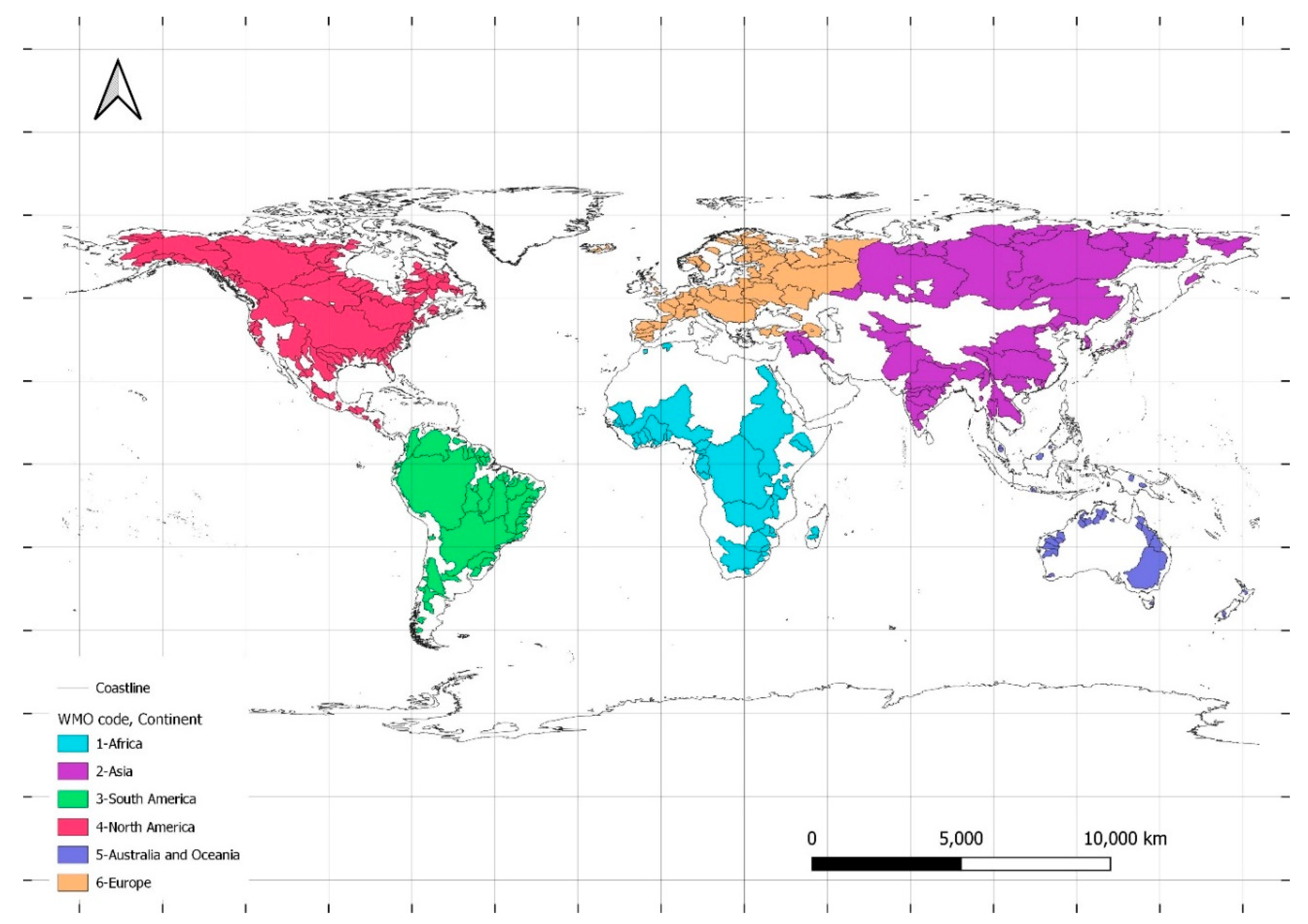
Figure 2.
Polarisation measure for monthly precipitation totals of the period 1901 to 2010.
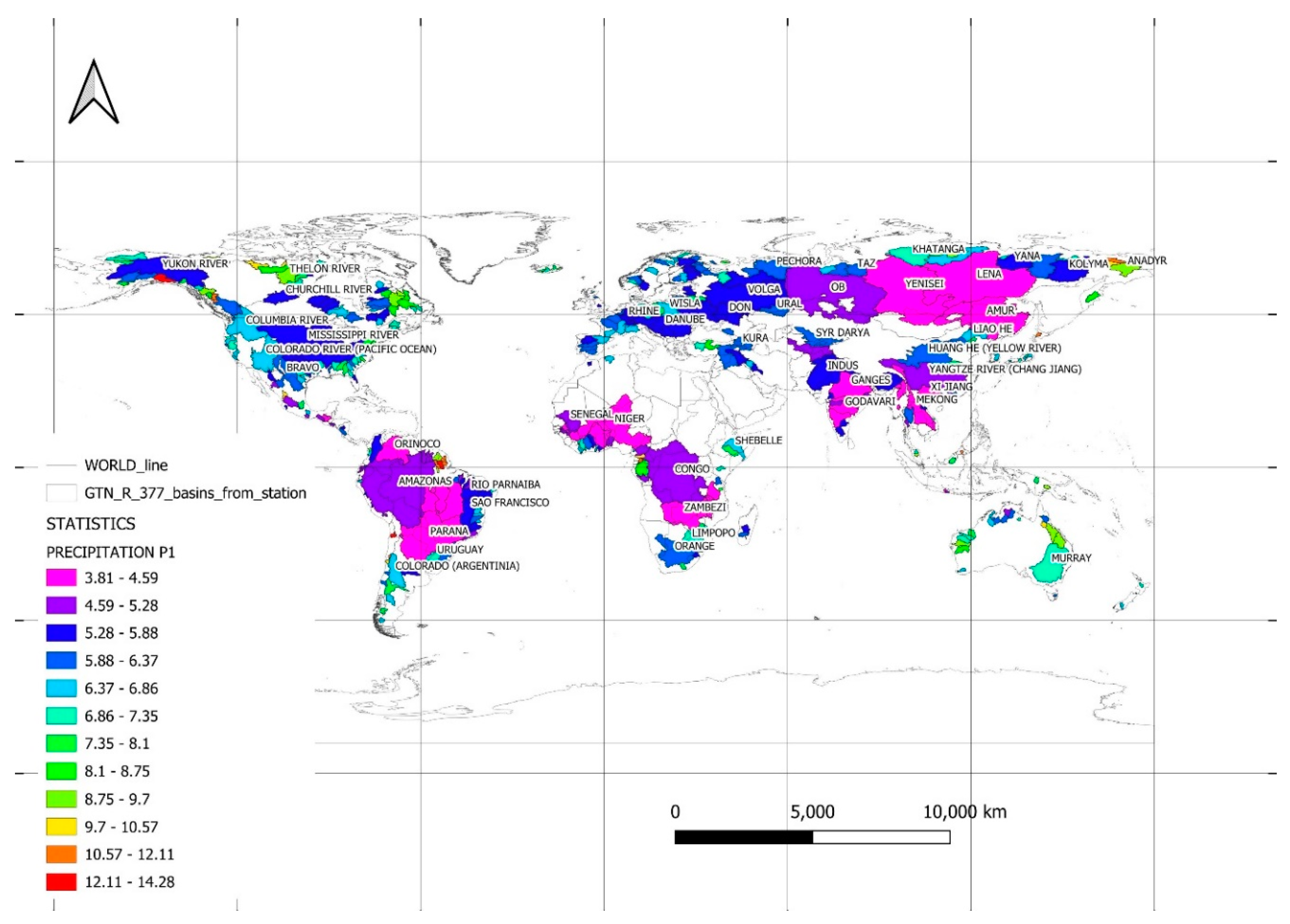
Figure 3.
Watersheds in which significant polarisation trends were identified for monthly precipitation sums during the period from 1901 to 2010 at a significance level of 5%.
Figure 3.
Watersheds in which significant polarisation trends were identified for monthly precipitation sums during the period from 1901 to 2010 at a significance level of 5%.
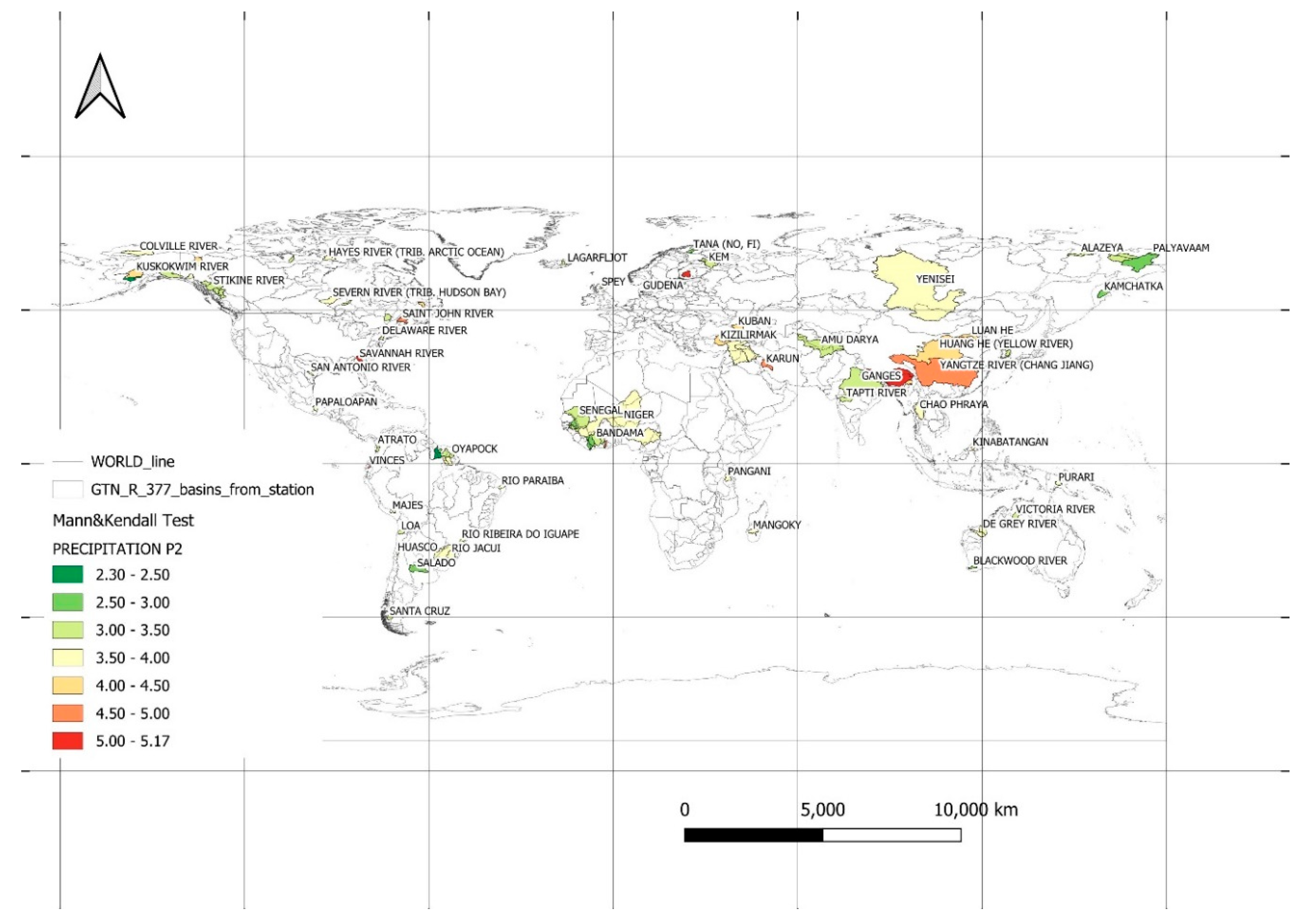
Figure 4.
Watersheds in which change points in the trend of factors related to precipitation polarisation for monthly precipitation sums during the period from 1901 to 2010 were identified at a significance level of 5%.
Figure 4.
Watersheds in which change points in the trend of factors related to precipitation polarisation for monthly precipitation sums during the period from 1901 to 2010 were identified at a significance level of 5%.
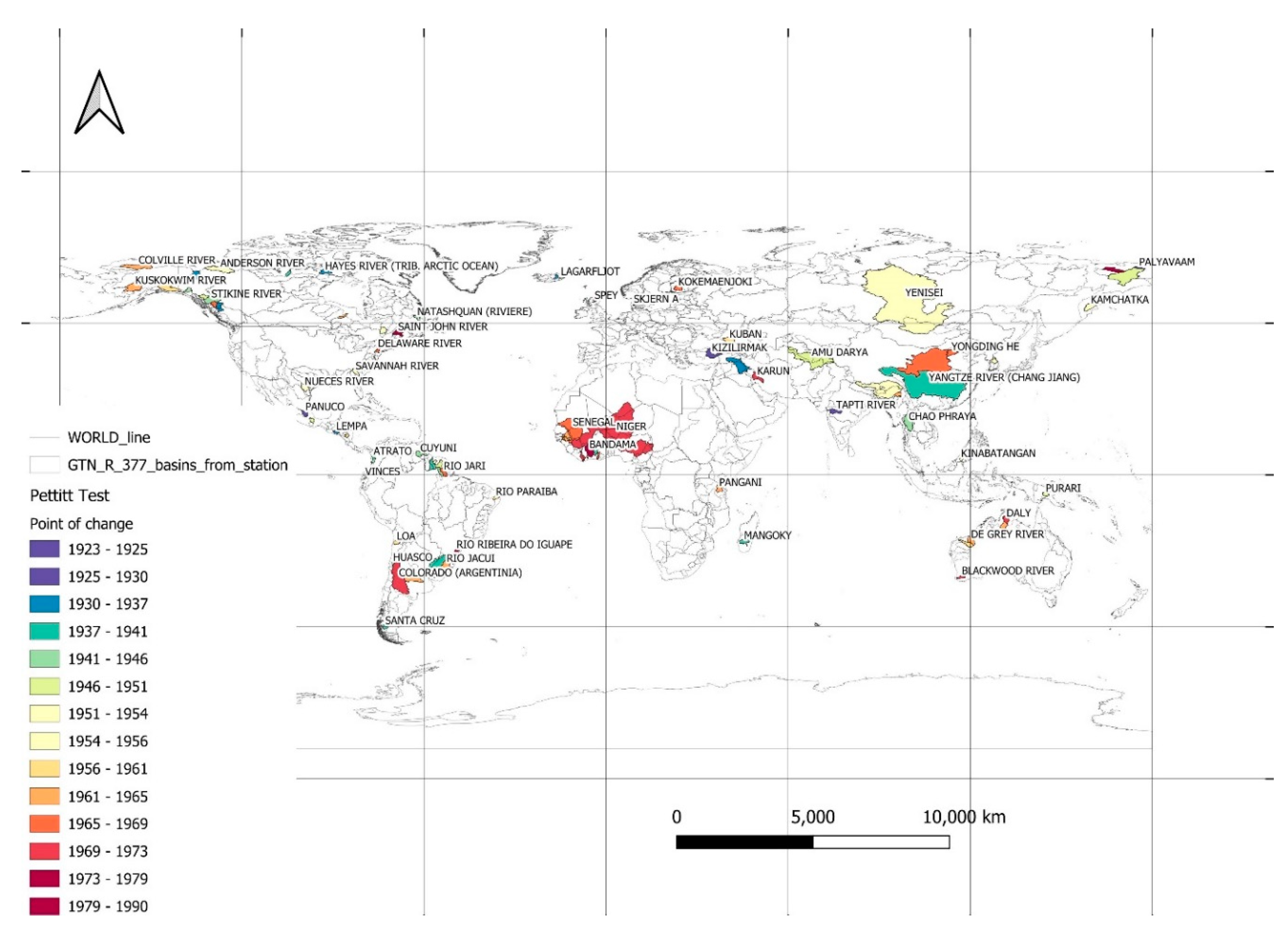
Figure 5.
Polarisation measure P1 for monthly temperature totals of the period 1901 to 2010.
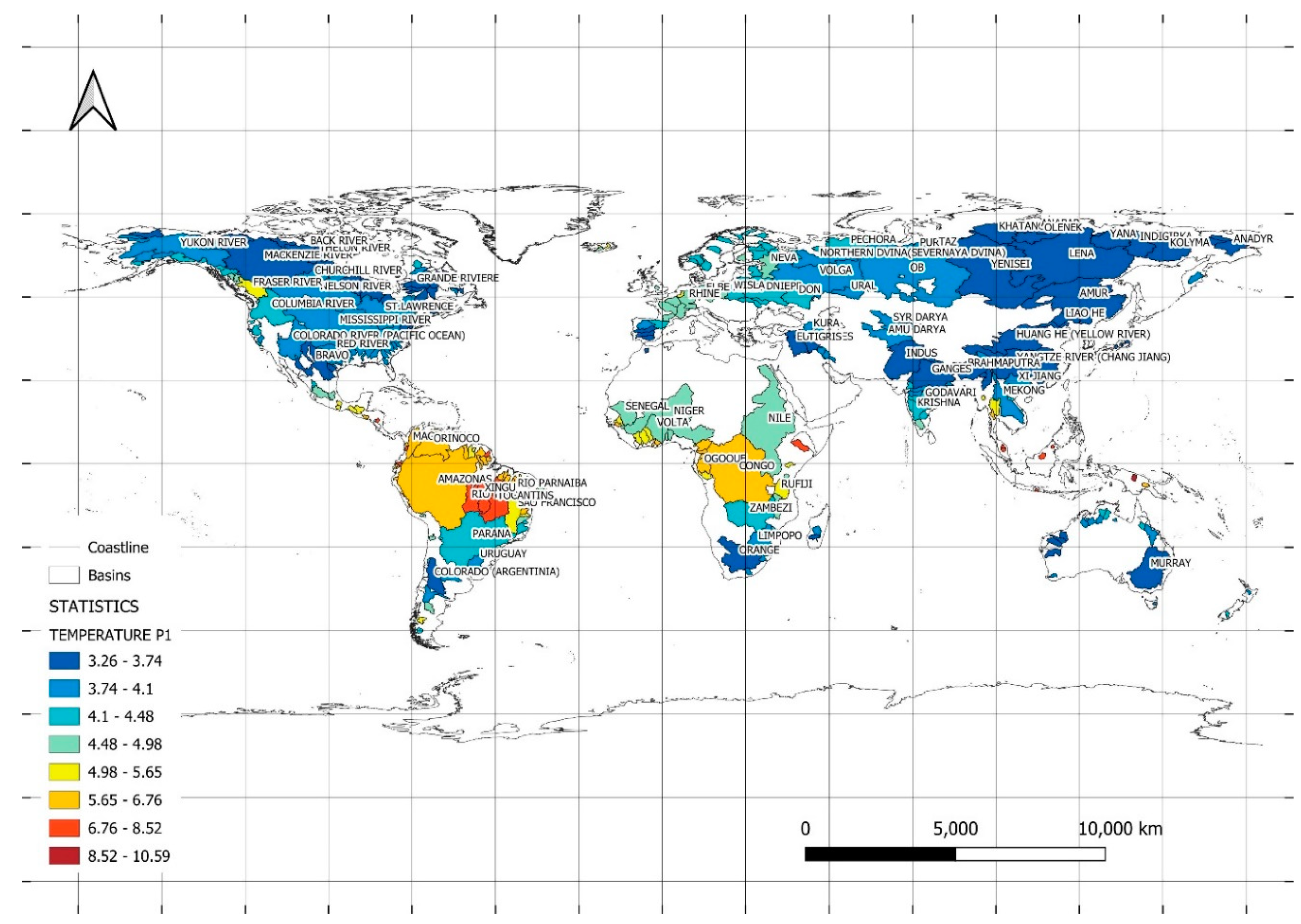
Figure 6.
Watersheds in which significant polarisation trends were identified for monthly mean temperatures during the period from 1901 to 2010 at a significance level of 5%.
Figure 6.
Watersheds in which significant polarisation trends were identified for monthly mean temperatures during the period from 1901 to 2010 at a significance level of 5%.
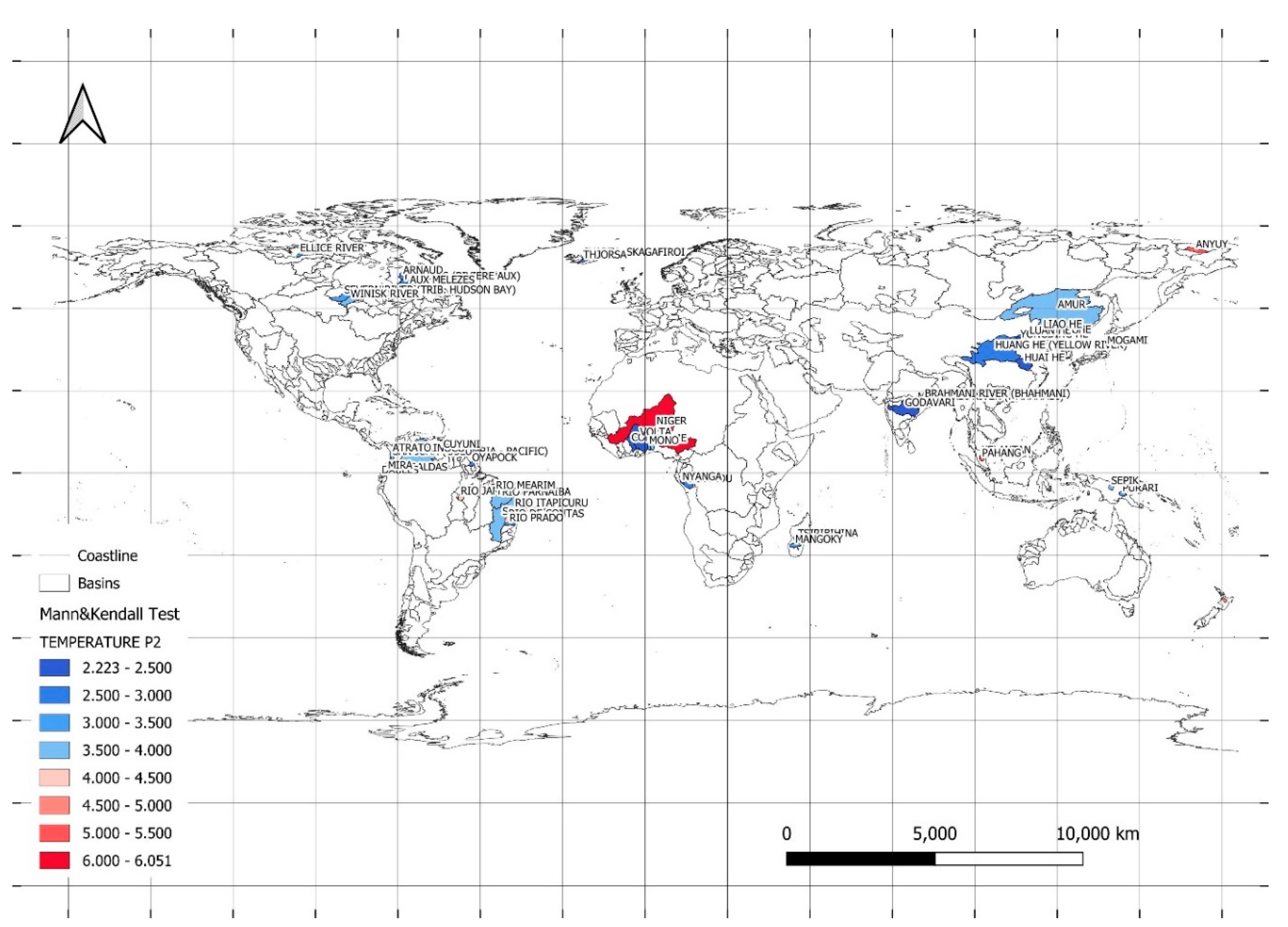
Figure 7.
Watersheds in which change points in the trend of factors related to temperature polarisation for monthly mean temperatures during the period from 1901 to 2010 were identified at a significance level of 5%.
Figure 7.
Watersheds in which change points in the trend of factors related to temperature polarisation for monthly mean temperatures during the period from 1901 to 2010 were identified at a significance level of 5%.
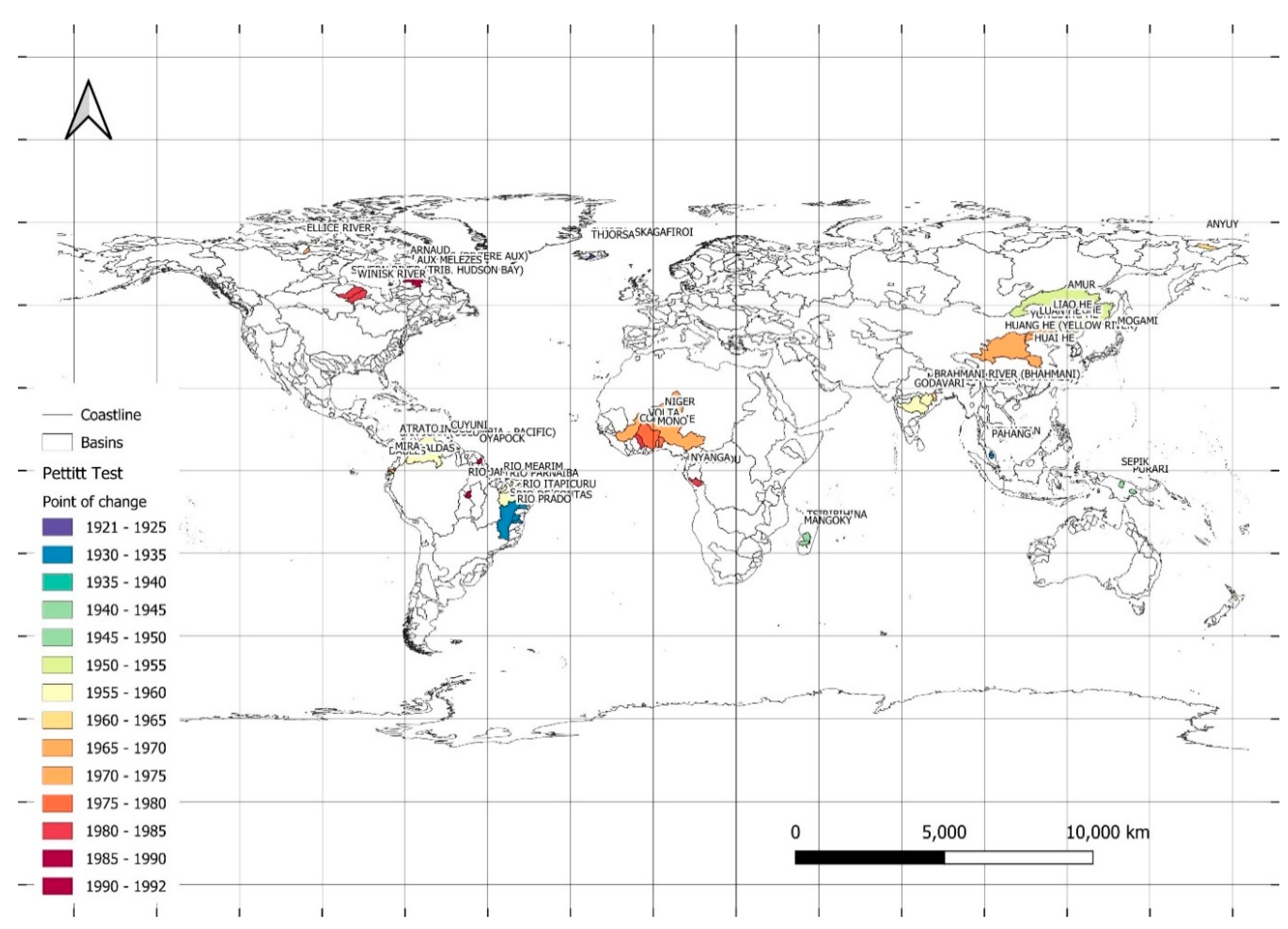
Figure 8.
A picture of polarisation phenomena in the area of precipitation and temperature, taking into account WMO regions. Quadrant I - both measures are increasing. Quadrant II - P2 measure of precipitation is decreasing, P2 measure of temperatures is increasing. Quarter III - both measures are decreasing. Quarter IV - measure P2 of precipitation is increasing, measure P2 of temperatures is decreasing.
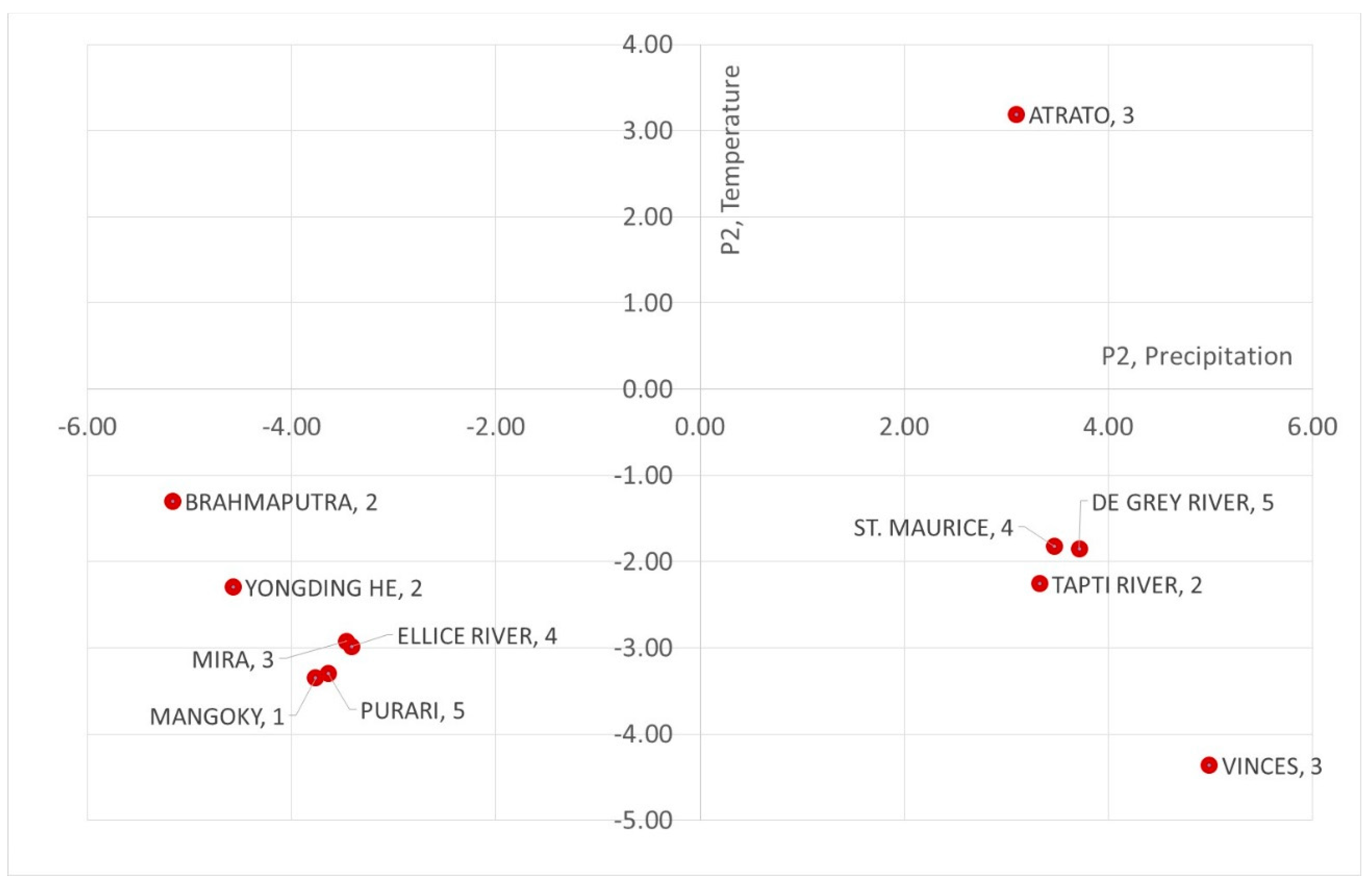

Table 1.
Table 1. Areas covered by the analysis.
| Region WMO | Continent | Land area | Area catchment | Coverage of the continents |
| WMO_REG | 106 km2 | 106 km2 | % | |
| 1 | Africa | 30.3 | 8.43 | 27.83% |
| 2 | Asia | 44.3 | 20.3 | 45.86% |
| 3 | South America | 17.8 | 12.6 | 70.57% |
| 4 | North America | 24.2 | 13.0 | 53.87% |
| Antarctica | 13.1 | 0.0 | 0.00% | |
| 5 | Australia and Oceania | 8.5 | 1.1 | 13.07% |
| 6 | Europe | 10.5 | 6.7 | 64.10% |
| Total land area | 148.7 | 65.1 | 43.77% | |
| Earth, total | 509.9 | 65.1 | 12.76% |
Disclaimer/Publisher’s Note: The statements, opinions and data contained in all publications are solely those of the individual author(s) and contributor(s) and not of MDPI and/or the editor(s). MDPI and/or the editor(s) disclaim responsibility for any injury to people or property resulting from any ideas, methods, instructions or products referred to in the content. |
© 2023 by the authors. Licensee MDPI, Basel, Switzerland. This article is an open access article distributed under the terms and conditions of the Creative Commons Attribution (CC BY) license (http://creativecommons.org/licenses/by/4.0/).
Copyright: This open access article is published under a Creative Commons CC BY 4.0 license, which permit the free download, distribution, and reuse, provided that the author and preprint are cited in any reuse.


