
Submitted:
20 July 2023
Posted:
21 July 2023
You are already at the latest version
Abstract
This study aims to identify the optimal combination of microphysics (MP) and cumulus (CU) parameterization schemes for accurately simulating heavy to violet rainfall events associated with Tropical Cyclones (TCs) and atmospheric disturbances in Thailand using the coupled Weather Research and Forecasting (WRF) and Regional Oceanic Model (ROMS), hereafter referred to as WRF-ROMS. Three CU schemes, namely Betts–Miller–Janjic (BMJ), Grell 3D Ensemble (G3), and Kain–Fritsch (KF), along with three MP schemes, namely Eta (ETA), Purdue Lin (LIN), and WRF Single-moment 3-class (WSM3), are selected for the sensitivity analysis. Seven instances of heavy to violent rainfall in Thailand, occurring during summer season of 2020 and associated with tropical storms and atmospheric disturbances, are simulated using all possible combinations of the chosen physics schemes. The simulated rain intensities are compared against observations from the National Hydroinformatics Data Center. Performance was assessed using the Probability of Detection (POD), False Alarm Ratio (FAR), and Critical Success Index (CSI) metrics. The models showed proficiency in predicting light to moderate rainfall, with certain combinations performing better in specific rainfall categories. However, forecasting heavy and violent rainfall proved challenging for all models and lead-time forecasts. Specific combinations, particularly those incorporating the KF scheme, demonstrated superior prediction of heavy to violent rainfall. The FAR values increased with lead-time and rain intensity, and the KF scheme combinations showed improved predictions of intense rainfall with lower FAR values. The CSI values indicated comparable performance between the control model and combination models across light to heavy rain categories, with the KF scheme showing better predictions for longer lead-times. However, accurately predicting intense rainfall remained limited. These findings highlight the need for further improvements, including refining model parameters and exploring advanced techniques to enhance accuracy and skill, particularly for longer-term forecasts. Sub-seasonal to seasonal prediction should be considered to extend forecast capabilities.
Keywords:
Heavy rainfall prediction
; Coupled WRF-ROMS
; Thailand
; Tropical cyclones and atmospheric disturbances
1. Introduction
Atmospheric disturbances and tropical storms have a significant impact on heavy rainfall due to their ability to transport moisture, generate upward motion, create convergence zones, interact with topography, persist for extended periods, release energy, and thrive in atmospherically unstable conditions. Typically, tropical storms originate from the highly energetic conditions prevailing over warm tropical oceans [1]. The warming of oceanic waters plays a pivotal role in cyclogenesis, as well as the subsequent intensification of tropical cyclones. This intensification is influenced by various factors, including the intensity of steering flows, the positioning of cyclonic circulation, atmospheric stability, and wind shear conditions [2,3,4].
The Indochina Peninsula (IP) is geographically located in Southeast Asia, making it prone to tropical storms and typhoons. The region is influenced by the South China Sea (SCS) and the Bay of Bengal (BoB), recognized as breeding grounds for tropical cyclones [5,6,7]. The SCS exhibits elevated frequencies of tropical storms due to the presence of low-level cyclonic circulation and their westward propagation towards the BoB. Consequently, this movement significantly affects extreme rainfall events over the IP sub-region during the late rainy season [8,9]. The IP generally experiences a tropical cyclone season from May to November, with peak activity concentrated between July and October, resulting in heavy rainfall, strong winds, and potential flooding. Additionally, heavy rainfall in the region can be induced by monsoon depressions along the monsoon trough. The frequency and intensity of tropical storms vary annually, influenced by regional and global climate patterns, including the El Niño-Southern Oscillation (ENSO), sea surface temperatures (SST), and atmospheric conditions [10].
Thailand, located centrally within the IP region, has consistently experienced severe and devastating flooding events on an interannual basis, primarily due to heavy rainfall associated with atmospheric disturbances. These events have resulted in significant socio-economic damage. Historical records reveal that catastrophic floods in Thailand have typically coincided with synoptic conditions, particularly tropical storms, renowned for their capacity to generate extreme weather, flooding, and storm surge [11,12,13,14,15]. Therefore, precise prediction of these high-impact weather events is vital for effective preparedness, early warning systems, and the implementation of disaster management strategies, which are crucial in mitigating the potential impacts of tropical storms on the region.
In recent decades, dynamic numerical forecast models have significantly advanced, effectively integrating atmospheric, surface, and subsurface processes, thereby extending the forecast period for tropical storms and flood events [16,17,18,19]. This progress can be attributed to improved understanding of physical processes, refined parameterizations, enhanced data assimilation techniques, the availability of high-resolution observations, increased computational capabilities, and international collaboration and data sharing [20,21,22,23,24]. However, current dynamic forecast models still have limitations in efficiently predicting tropical storms and capturing the intricate interplay between complex oceanic conditions and air-sea interactions that modulate heavy rainfall on a regional scale [25,26,27]. These models entail complexity and necessitate numerous assumptions regarding cloud formation and its interaction with the atmosphere. These assumptions are typically encompassed within microphysical (MP) and cumulus (CU) parameterization schemes.
In numerical atmospheric models, the CU parameterization scheme plays a vital role in accounting for sub-grid scale cloud-radiation interactions, which are intricately connected to the vertical redistribution of atmospheric heat and moisture tendencies [28,29]. Previous sensitivity studies have demonstrated the significant impact of cumulus parameterization on simulated rainfall during tropical storms in Southeast Asia, specifically in Thailand (Raktham et al., 2015; Wangwongchai et al., 2010; Chotamonsak et al., 2012). Furthermore, the microphysical (MP) parameterization, which influences the sub-grid scale vertical flux of cloud and sedimentation processes of hydrometeors, also plays a crucial role at the regional level [30,31]. These effects on tropical cyclone intensity, such as moisture distribution, latent heating, and convection, are critical for improving simulations during tropical storms in the surrounding areas of Thailand [32,33,34]. Microphysics scheme can also provide a better representation of evaporation processes from frozen hydrometeors and a substantial quantity of liquid hydrometeors, resulting in improved latent heat release in storms and a correlated increase in precipitation amounts and distribution [35]. The significance of CU and MP parameterization in simulating tropical storms and regional rainfall has been highlighted in previous studies. However, it is important to note that the existing research primarily focuses on specific tropical storm events, resulting in a limited number of cases and insufficient systematic analyses regarding the temporal and spatial consistency associated with regional rainfall. Furthermore, it is important to highlight the limitations of previous studies. One notable limitation is that the models employed in these studies are primarily based on standalone atmospheric modeling, neglecting the crucial role of air-sea interaction, which plays a vital role in modulating the behavior and characteristics of tropical storms.
Based on the aforementioned considerations, it is crucial to address three key aspects when enhancing the simulation model. These include incorporating the air-sea interaction process into the simulation, exploring the sensitivity of CU and MP parameterization for improved short-term rainfall forecasting during tropical storms, and refining the boundary and physical conditions. Consequently, the objective of this study is to investigate the relative sensitivities of various CU and MP parameterization schemes in simulating spatiotemporal variations of rainfall during tropical storm events in Thailand, utilizing the WRF-ROMS model. Specifically, this paper focuses on simulating heavy rainfall patterns in Thailand during tropical storm events at a high horizontal resolution of 3-km and examining the forecast skill associated with different CU and MP schemes.
Section 2 provides a detailed description of the model configuration and the design of sensitivity experiments conducted in this study. Section 3 outlines the methodology for selecting tropical storm events, the observational data utilized for evaluation, and the verification methods employed. In Section 4, we evaluate the forecast skill of rainfall in various regions of Thailand across four distinct rainfall categories and present a comprehensive discussion of the results. Finally, Section 5 summarizes the main findings derived from this study.
2. Materials and Methods
2.1. Oserved rainfall data
The rainfall intensities simulated in this study were compared to observations obtained from the National Hydroinformatics Data Center (NHC), which serves as a pivotal repository for hydrological and meteorological data in Thailand. The NHC has emerged as a vital hub for water resource management, disaster preparedness, and scientific research by establishing data linkages with over 50 agencies (https://www.thaiwater.net/).
For our analysis, we collected daily rainfall data from a comprehensive network of 1234 NHC stations. These stations were distributed across different regions of Thailand, with 213 stations in the Central region, 119 stations in the Western region, 49 stations in the Eastern region, 188 stations in the Northeastern region, 422 stations in the Northern region, and 243 stations in the Southern region. The spatial distribution of the NHC stations utilized in this study can be visualized in Figure 1.
2.2. Model configurations and experiment designs
2.2.1. Model description
In this study, we employed a coupled modeling system, so called Coupled Ocean-Atmosphere-Wave-Sediment Transport modeling system (COAWST), that originally developed at the United States Geological Survey (USGS) [36,37]. In the COAWST, interactions of different physical processes of the Earth’s components, i.e., ocean, atmosphere, wave, sediment transport, and sea-ice are integrated into the modeling system. The coupled modeling system is open-source, free of charge and available online at https://code.usgs.gov/coawstmodel/COAWST.
The COAWST system utilizes the Regional Ocean Modeling System (ROMS) as a functional modeling framework to estimate the state of the ocean. ROMS is a numerical model based on a free-surface, terrain-following approach, employing hydrostatic and Boussinesq approximations [38,39]. It provides a means to simulate the ocean's behavior and processes. Concurrently, the Weather Research and Forecasting (WRF) Model is employed to estimate atmospheric variables. WRF is an advanced mesoscale model based on a non-hydrostatic atmospheric formulation, utilizing terrain-following vertical coordinates [40]. Widely employed by the scientific community, the WRF model facilitates diverse research studies and operational applications, for instances, potential solar and wind energy resources, localized flood hazards, short-term weather forecast, and climate studies [41,42,43,44,45,46]. It is important to acknowledge that the specific formulations and parameterizations of cumulus schemes in the WRF model may vary, with different schemes prioritizing specific tendencies. Consequently, researchers and modelers frequently calibrate these schemes using observational data to enhance their representation of real-world atmospheric processes, particularly when coupled with oceanic models.
The WRF-ROMS coupling allows for the simulation of interactions between the atmosphere and the ocean, which can be important for understanding weather patterns and their effects on oceanic processes. This model has been used in a variety of applications, including forecasting ocean conditions and predicting the impacts of storms on coastal regions. Torsri et al. [47] conducted an initial research endeavor aimed at evaluating rainfall simulation in Thailand by comparing coupled and non-coupled approaches. Their findings suggested that incorporating air-sea interaction in the modeling framework yielded superior results compared to the non-coupled approach. However, the study did not specifically investigate the impacts of different cumulus and microphysics options within the WRF model. Consequently, the examination of these factors remains a pertinent challenge that necessitates further investigation.
Note that the modeling system used here is the COAWST version 3.2, which is the same version being officially routinely operated at the Hydro-Informatics Institute, Ministry of Higher Education, Science, Research and Innovation, Thailand since 2016 for short-term weather forecast system (7 days in advance). So far, the WRF-ROMS forecasted results are publicly available online at https://www.thaiwater.net/weather/ and also disseminated to stakeholders and researcher that related to disaster prevention, early warning, and water resource management in Thailand and some ASEAN countries (https:://www.aseanwater.net/). This study focuses on examining synoptic weather systems and rainfall forecasts, with particular attention given to the influence of air-sea interactions. To facilitate this investigation, the WRF is coupled with the ROMS. While certain microscale processes (i.e., wave and sediment components) occurring at scales smaller than the model's grid cells can be disregarded, other important components are considered.
2.2.2. Selection of heavy rainfall events
In 2020, Thailand experienced several instances of heavy rainfall, primarily attributed to atmospheric disturbances. In this year, the weather condition of Thailand can be attributed to the significant impact of storms. These disturbances included events such as Sinlaku in August, tropical storm Noul in September, and typhoon Molave in October. These occurrences resulted in significant rainfall throughout the country, particularly in the northern regions, leading to severe damage to infrastructure, properties, and agricultural resources [46]. Apart from atmospheric disturbances, heavy rainfall in Thailand can also be caused by a low-pressure zone known as the monsoon trough. During the summer monsoon season, this trough shifts northward, resulting in heavy rainfall and wet conditions in the northern parts of Thailand. Conversely, during the winter monsoon season, the trough shifts southward, leading to drier conditions in the north and increased precipitation in southern Thailand. Hence, selection of events that occurred during summer months in 2020 is a suitable choice for verifying prediction skills with different combinations of cumulus and microphysics options due to the following reasons: (1) variety of atmospheric disturbances that exhibited different characteristics and intensities, providing a diverse set of conditions to evaluate the prediction skill of different cumulus and microphysics options and (2) significant impact on rainfall by which the selected events resulted in substantial rainfall across Thailand.
Here, we conducted a case study focusing on seven significant heavy rainfall events that took place in 2020, each of which was associated with atmospheric disturbances (i.e., tropical storms, depressions, low pressure, and monsoon troughs). These disturbances either moved through or formed within a defined geographical area (0.0−25.0°N, 90.0°E−120.0°E), which is known to potentially impact on weather conditions of Thailand [48]. Detailed information regarding each selected event is provided in Table 1. To analyze the behavior of each event, we also plot the spatial distribution of rainfall on the target date alongside its corresponding synoptic weather chart in Figure 2. A concise summary of each selected event is provided below:
On June 14th (Event 1), Thailand experienced heavy rainfall, particularly in the northern, northeastern, central, and eastern regions, with rain intensity reaching a maximum of 90.0 mm in certain areas. This rainfall event was caused by a tropical depression named Nuri, which originated in the eastern part of the Philippines and passed through the upper part of the SCS (Figure 2a). Subsequently, on August 1st, another notable heavy rainfall event occurred due to Tropical Depression Sinlakul (Event 2). The Sinlakul initially formed as a tropical depression over the northern SCS on the morning of July 31st. It further intensified into a tropical storm and gradually moved towards the northern regions of Vietnam over the following days. Before entering Thailand, Sinlakul weakened and transitioned into a tropical depression. As Sinlakul traversed through Thailand, in conjunction with the presence of the monsoon trough over the region, these combined weather conditions resulted in heavy to violent rainfall, reaching the highest intensity of about 150.0 mm, primarily northeastern Thailand (Figure 2b). As a result, the area experienced widespread flooding, landslides, rapid water surges, forest runoff, and extensive damage to properties [46].
On the 18th of the follwing month (Event 3), Thailand encountered a notable increase in rainfall, characterized by heavy to very heavy rainfall in upper sub-regions (Figure 1c). The highest recorded intensity of 243.8 mm was observed in Phetchabun Province, in the North [48]. This increase in rainfall was attributed to the impact of a tropical depression that intensified into a tropical storm (TS) and was internationally named "Noul". The storm's trajectory moved towards northeastern Thailand, passing through the central and eastern regions and extending into certain areas of the western regions (Figure 2c). As a result, widespread flooding and flash floods occurred in multiple areas. On October 16th (Event 4), a combined effect of Tropical Depression (TD) moving westward from the central SCS towards Vietnam, along with the intensified monsoon trough sweeping across the central, eastern, and upper regions of southern Thailand. This meteorological phenomenon led to substantial rainfall in these areas of Thailand, with certain locations experiencing rainfall exceeding 90.0 mm (Figure 2d) (Figure 2d).
During the later months (November to December), corresponding to the winter season in Thailand when the Northeast monsoon prevails, there was a frequent occurrence of heavy rainfall events in the southern Thailand (Events 5 to 7). These events were primarily concentrated along the east coast of the South, where heavy to violent rainfall was commonly observed (refer to Figure 2e-f). These weather patterns were attributed to the formation of a low-pressure system induced by a tropical storm in the SCS, and occasionally influenced by a tropical cyclone in the BoB.
To facilitate model integration, we established three distinct initial dates for the study: the date corresponding to heavy rainfall occurrence (lead-0), the date preceding the event (lead-1), and the date further preceding the event (lead-2) (refer to Table 1 for specific information). Subsequently, we conducted model integration and simulation for a period of 24 hours, 48 hours, and 72 hours for each of the aforementioned lead times to simulate the target date of each event. In doing this, the diverse range of atmospheric patterns observed in the selected events provides a solid foundation for evaluating the effectiveness and accuracy of different cumulus and microphysics parameterizations in predicting and capturing heavy to violent rainfall patterns across Thailand.
2.2.3. Combinations of CU and MP
It is acknowledged that estimation of rainfall over a certain region in an atmospheric model is strongly dependent on CU and MP parameterizations. Many studies have revealed that applying different combinations of cumulus and microphysics options in a model for a region can yield different results [49,50]. In this study, we designed, in total, 9 combinations of CU and MP parameterizations by which three CU schemes, namely Betts–Miller–Janjic (BMJ), Grell 3D Ensemble (G3), and Kain–Fritsch (KF) along with three MP schemes, namely Eta Ferrier (ETA), Purdue Lin (LIN), and WRF Single-moment 3-class (WSM3), are selected for the sensitivity analysis. It is important to note that the combination of the BMJ and ETA parameterization is denoted as the control run (CTL) in this study. The selection of this particular combination as the control run is justified by its prior verification in Torsri et. al. [47], as well as its ongoing utilization within the current operational system at the Hydro-Informatic Institute, Thailand. Consequently, it serves as a reference against which other combinations are compared in our analysis.
A summary of combinations are given in Table 2. The seven instances of heavy to violent rainfall in Thailand (listed in Table 1), occurring during June to December of 2020 and associated with tropical storms and atmospheric disturbances, are simulated using all possible combinations of the chosen physics schemes.
The BMJ, G3, and KF schemes are widely used in atmospheric modeling and have been extensively evaluated and tested in tropical regions [57,58,59,60]. The main differences among these schemes lie in the complexity of the parameterization and the treatment of convective processes. BMJ is relatively simple, using a relaxed Arakawa-Schubert closure. G3 employs an ensemble-based approach with multiple convective plumes, while KF operates on a higher-resolution grid and includes a downdraft parameterization. Overall, while all three schemes consider the transport of moisture within cumulus convection, they may have different parameterizations for specific processes such as detrainment, entrainment, and vertical mixing for treatment of moisture tendencies (Table 3). The assumptions made in each scheme affect how moisture tendencies are represented and contribute to the overall moisture budget within the model grid cell [61].
The choice of microphysics is of utmost importance due to its significant impact on the accurate representation of key atmospheric processes, including water vapor, cloud droplets, ice particles, rain, and other hydrometeors within the atmosphere. The precise simulation of these processes is directly linked to the reliability and accuracy of weather forecasts and simulations. In order to comprehensively evaluate the representation of interactions between cumulus convection and microphysical processes, it is essential to consider a diverse range of microphysics options in conjunction with the selected CU schemes. For this study, we have specifically chosen three MP schemes, namely ETA, LIN, and WSM3, to describe the distinct interactions among water vapor, cloud droplets, ice particles, rain, and other hydrometeors within the atmosphere (refer to Table 3 for details).
In this study, our primary focus lies in predicting heavy rainfall associated with atmospheric disturbances, particularly in tropical regions. For this purpose, the chosen CU and MP schemes have demonstrated superior performance in situations involving tropical atmospheric disturbances [49,50,57,58,59,62,63,64]. However, it is important to note that the effectiveness of a particular combination of CU and MP options in one region does not guarantee similar performance in another region. Therefore, prior to the application of any CU and MP scheme in a specific area of interest, conducting a sensitivity analysis on the parameterization is essential. This analysis allows for a thorough assessment of the performance and suitability of CU and MP schemes in capturing the unique characteristics and dynamics of the target region.
2.2.4. Modeling domains
In this study, we employed COAWST version 3.2, specifically activating the coupling between the WRF model and ROMS, to simulate a target selection of seven rainfall events (refer to Table 1). Our configuration of the WRF model consisted of three nested domains with respective resolutions of 27 km (D01), 9 km (D02), and 3 km (D03), accompanied by 33 vertical levels. The outermost domain encompassed a significant area of Greater East Asia, encompassing South Asia, Southeast Asia, and East Asia, while the finest domain covered the entirety of Thailand, as illustrated in Figure 3a. The ROMS domain with a horizontal resolution of 25 km2 and with 15 vertical layers spanned from 70°E to 180°E and 20°S to 35°N, ensuring comprehensive coverage of the influences of SST on atmospheric processes in the BoB and the SCS (Figure 3b).
Each of the target date simulation, the WRF model was initialized and driven with three different model lead times as defined in Table 1. Meteorological information being used for initialization and driving forces of the WRF model was obtained from the 6-hr Global Forecast System (GFS), which developed by the National Centers for Environmental Prediction (NCEP) and freely available online at https://www.emc.ncep.noaa.gov/emc/pages/numerical_forecast_systems/gfs.php [65]. Initial conditions for the ROMS model, fields of currents, salinity, and temperature are obtained from the global HYCOM simulation via https://www.hycom.org/dataserver/gofs-3pt1/analysis [66]. In this configuration, the ROMS model exchanges SST with WRF every 3600 seconds. Then, the atmospheric model utilizes the received SST information as a boundary condition and reciprocally sends turbulent heat fluxes to the oceanic model [37]. By adopting this approach, ROMS can provides high-resolution and dynamically consistent SST updates. Moreover, the heat fluxes transmitted from WRF to ROMS are based on the SST received from ROMS, ensuring a coherent treatment of energy and momentum exchange [67].
2.3. Statistical evaluation metrics
According to the definition given by the Thai Meteorological Department [68], daily rainfall in the region can be classified into five distinct categories: (1) trace rain (< 0.1 mm), (2) light rain (0.1−10.0 mm), (3) moderate rain (10.1−35.0 mm), (4) heavy rain (35.1−90.0 mm), and (5) very heavy or violent rain (> 90.1 mm). The main objective of this study is to assess the impacts of CP and MP on the estimation of high-impact weather events, specifically focusing on heavy (> 35.0−90.0 mm/day) and violent rainfall (> 90.0 mm/day) categories.
For statistical metrics, we employed the probability of detection (POD), false alarm (FAR), and critical success index (CSI), known as treat score (TS) for model evaluation. The equations for these metrics are presented below:
, and
where:
- Hits refer to the number of correctly detected events.
- Misses refer to the number of events that were present but went undetected.
- False Alarms refer to the number of incorrect detections or false positives.
The POD is a crucial metric for Numerical Weather Prediction (NWP) by which it can provide an objective measure of the model's ability to accurately predict the occurrence of specific weather phenomena or events. Hence, the metric is particularly important for high-impact weather events, such as severe storms or heavy rainfall, which can have significant societal and economic consequences, making their accurate prediction of utmost importance. Evaluating the POD allows forecasters and researchers to assess the model's performance in capturing and predicting such high-impact events, which aids in decision-making and risk mitigation.
To provide a comprehensive evaluation of the model's performance, by considering POD along with other metrics, forecasters and researchers can assess not only the model's detection capability but also its ability to minimize false alarms and capture the overall forecast skill. Furthermore, in order to gain a more comprehensive understanding of the model’s prediction skill, the analysis is stratified into six distinct regions of Thailand (see Figure 3) considering regional average of the evaluation metrics.
Note that, for model evaluation, a systematic approach is employed. Firstly, observed and simulated rain intensity data, specifically for heavy and violent categories, are extracted for each target date. The simulated values are then compared against the corresponding observed values for the seven selected events. Consequently, the statistical values presented here represent an overall assessment of the model's performance across all events rather than a specific case. To maintain consistency, the observed rainfall data is interpolated to match the highest horizontal resolution of the model used in the analysis (3×3 km2). This ensures that both observed and simulated datasets undergo identical analysis procedures, facilitating an objective and unbiased evaluation.
3. Results
3.1. Probabilty of detection (POD) of rainfall forecast over Thailand during the selected events
Figure 4 shows the POD for rainfall forecasts in Thailand during the selected events. We categorize the forecasts into four distinct rainfall categories, as defined by the daily TMD criteria and compared with the observation with primary focusing on the accurate prediction of heavy and violent rainfall events.
In the case of light rain, employing a specific set of BMJ combinations exhibits a higher POD across all lead-time forecasts, as depicted in Figure 4a-c. It is noteworthy that the BMJ combination, particularly with the more complex MP schemes such as LIN and WSM3, exhibits a slightly superior POD performance ranging from 10.0-20.0% compared to CTRL, depending on the lead-time. On the other hand, the POD values for other combinations remain comparable to CTRL for the initial lead-time forecast, with a slight decrease of 5.0-10.0% as the lead-time forecast increases. In the case of moderate rainfall, the CTRL and a specific set of G3 combinations demonstrate superior performance, accurately forecasting the POD at around 45.0−50.0%. Conversely, lower skill is observed in other combinations, particularly in a set of KF combinations.
When predicting heavy rainfall, the model exhibits improved results (in comparison to CTRL) by utilizing a specific set of G3 and KF combinations, especially when combined with ETA and LIN microphysical options for all lead-times. Notably, the model utilizing the G3 and KF combinations demonstrates comparable performance in the first two lead-times, while consistently exhibiting superior performance in all subsequent lead-time forecasts. In the case of violent rainfall forecasts, it is evident that a combination of BMJ, G3, and KF, along with LIN microphysics, outperforms other combinations with the highest POD achieved when combined with KF (approximately 80.0%) for lead-0. For subsequent lead-times, the set of KF combinations consistently exhibits high prediction skill with POD values exceeding 60.0%, while lower predictions (POD < 30.0%) are observed in the other combinations.
3.2. False alarm ratio (FAR) of rainfall forecast over Thailand during the selected events
To quantify the frequency of false alarms or inaccurate predictions of rainfall occurrence, we calculated the FAR for each rainfall category, as depicted in Figure 5. In general, the FAR values for the CTRL in predicting light to moderate rainfall are similar to those obtained from all combinations, with magnitudes ranging from 50% to 70%. Notably, both the CTRL and other combinations exhibit an increase in FAR as the lead-time forecast and rain intensity increase (Figure 5a-c). Regarding heavy rainfall, the FAR values for the CTRL and all combinations are comparable, with the highest FAR reaching 80% at a lead-time-2. Moreover, it is evident that the FAR is significantly higher in the BMJ combination set in capturing heavy rainfall compared to the others, while improved predictions of intense rainfall are observed in the KF scheme combinations, exhibiting lower FAR values, particularly for longer lead-time forecasts.
3.3. Critical succes index (CSI) of rainfall forecast over Thailand during the selected events
The CSI was calculated to assess the performance of rainfall forecasts and given in Figure 6. Note that a higher CSI value indicates a more skillful and accurate forecast. As seen, CTRL and all combinations are comparable in prediction of light rain to heavy rain categories in all lead-time forecasts (Figure 6a-c). By analyzing the CSI values, it was observed that the CTRL run and all combinations exhibited comparable performance in predicting rainfall across the categories of light to heavy rain, regardless of lead-time forecasts (Figure 6a-c). The CSI values revealed varying levels of success for the rainfall forecasts during the selected events. Specifically, light rain events demonstrated higher CSI values, particularly in the set of BMJ combinations (35.0−40.0%), followed by the set of KF combinations (30.0−35.0%), indicating a stronger agreement between the forecasted and observed rainfall occurrences compared to other rainfall categories. However, it is worth noting that the prediction skill of the CTRL decreased as the intensity of rainfall increased, particularly for violent rainfall, which exhibited very low skill (CSI < 10.0%) at higher lead-time forecasts (Figure 6c). It is noticed that the model consistently shows better prediction of heavy to violent rainfall in almost all lead-time forecasts when employing KF scheme, specifically in lead-time-1 and lead-time-2. However, the prediction of the intense rainfall categories is still limitted with CSI values less than 20.0%.
4. Discussion and conclusions
The study evaluated the performance of rainfall forecast models using a coupled modeling system, COAWST during selected events in Thailand based on the Probability of Detection (POD), False Alarm Ratio (FAR), and Critical Success Index (CSI) metrics. The results indicated both strengths and weaknesses in the models' performance. The models demonstrated proficient prediction of light to moderate rainfall, with certain combinations showing higher skill in specific scenarios. However, the prediction of heavy and violent rainfall proved more challenging, with limited success across all models and lead-time forecasts.
Regarding the POD, the model performance varied across different rainfall categories and lead-time forecasts. In the case of light rain, specific combinations, particularly the BMJ combinations with LIN and WSM3 microphysical options, exhibited higher POD values compared to the CTRL. However, other combinations showed comparable performance to CTRL, except for a slight decrease in POD as the lead-time increased. For moderate rainfall, CTRL and specific G3 combinations demonstrated superior performance with POD values around 45.0−50.0%. Conversely, the KF combinations showed lower skill in predicting moderate rainfall. For heavy rainfall, certain G3 and KF combinations, particularly when combined with ETA and LIN microphysical options, showed improved results compared to CTRL. In the case of violent rainfall, the combination of BMJ, G3, and KF, along with LIN microphysics, outperformed other combinations, especially when combined with KF for lead-0. The KF combinations consistently exhibited high prediction skill for subsequent lead-times, while lower predictions were observed in other combinations.
In terms of the FAR, both CTRL and the combination models showed similar performance in predicting light to moderate rainfall. The FAR values increased as the lead-time forecast, and rain intensity increased. For heavy rainfall, the FAR values were comparable between CTRL and the combination models, with the highest FAR observed at lead-time-2. The BMJ combinations showed higher FAR values in capturing heavy rainfall, while the KF scheme combinations exhibited improved predictions of intense rainfall with lower FAR values, particularly for longer lead-time forecasts.
The CSI analysis revealed that CTRL and the combination models exhibited comparable performance in predicting rainfall across light to heavy rain categories and various lead-time forecasts. Light rain events showed higher CSI values, particularly in the BMJ and KF combinations, indicating a stronger agreement between the forecasted and observed rainfall occurrences. However, the prediction skill of CTRL decreased as the intensity of rainfall increased, especially for violent rainfall, with very low CSI values at higher lead-time forecasts. It is worth noting that the KF scheme consistently showed better prediction of heavy to violent rainfall in almost all lead-time forecasts. However, the prediction of intense rainfall categories remained limited.
In summary, our analysis revealed that the KF scheme consistently demonstrated superior prediction of heavy to violent rainfall compared to other combinations, especially in longer lead-time forecasts. However, the models' ability to accurately forecast intense rainfall categories remained limited, as indicated by low CSI values. These findings provide valuable insights for future advancements in rainfall forecast models, specifically focusing on enhancing the prediction accuracy of heavy and violent rainfall events. Further research and development efforts should prioritize the refinement of model parameters and exploration of advanced techniques to improve forecast accuracy and skill, particularly for extending the forecast period to longer time scales, such as sub-seasonal to seasonal prediction.
Author Contributions
Conceptualization and methodology, K.T.; validation, K.T., A.F., P.P. and J.A.; formal analysis, R.S. and J.A.; investigation, K.T.; data curation, A.F., P.P. and R.S.; writing—original draft preparation, K.T.; visualization, A.F., P.P., and R.S.; funding acquisition, K.T.; writing—review and edit, K.S. All authors have read and agreed to the published version of the manuscript.
Funding
This research was funded by Science, Research and Innovation Promotion Fund (SRI), Thailand Science Research and Innovation (TSRI), grant number 48873, 160399, and 180529 under the Sub-Seasonal to Seasonal (S2S) Prediction Project for Disaster Risk Reduction and Water Management in Thailand (S2S-Thai Project).
Institutional Review Board Statement
Not applicable.
Informed Consent Statement
Not applicable.
Data Availability Statement
Reader can find data availability of the WRF-ROMS forecast and NHC via https://www.thaiwater.net/. For details of the meteorological data over Thailand, they can be approached by contacting K.T.
Acknowledgments
The authors sincerely thank the NHC for the daily rainfall station data and the USGS for availability of the COAWST modeling system. We also acknowledge the National Science and Technology Development Agency (NSTDA) Supercomputer Center (ThaiSC) for providing computing resources for this work.
Conflicts of Interest
The authors declare no conflict of interest.
References
- Gray, W.M. Global view of the origin of tropical disturbances and storms. Monthly Weather Review 1968, 96, 669–700. [Google Scholar] [CrossRef]
- Bruyère, C.L.; Holland, G.J.; Towler, E. Investigating the Use of a Genesis Potential Index for Tropical Cyclones in the North Atlantic Basin. Journal of Climate 2012, 25, 8611–8626. [Google Scholar] [CrossRef]
- Byers, H. Atmospheric turbulence and the wind structure near the surface of the Earth. General meteorology 1944. [Google Scholar]
- Emanuel, K.A. An Air-Sea Interaction Theory for Tropical Cyclones. Part I: Steady-State Maintenance. Journal of Atmospheric Sciences 1986, 43, 585–605. [Google Scholar] [CrossRef]
- Krishnamurti, T.N.; Molinari, J.; Pan, H.-l.; Wong, V. Downstream Amplification and Formation of Monsoon Disturbances. Monthly Weather Review 1977, 105, 1281–1297. [Google Scholar] [CrossRef]
- Saha, K.; Sanders, F.; Shukla, J. Westward Propagating Predecessors of Monsoon Depressions. Monthly Weather Review 1981, 109, 330–343. [Google Scholar] [CrossRef]
- Chen, T.-C.; Chen, J.-M. The 10–20-Day Mode of the 1979 Indian Monsoon: Its Relation with the Time Variation of Monsoon Rainfall. Monthly Weather Review 1993, 121, 2465–2482. [Google Scholar] [CrossRef]
- Takahashi, H.G.; Yasunari, T. Decreasing Trend in Rainfall over Indochina during the Late Summer Monsoon: Impact of Tropical Cyclones. Journal of the Meteorological Society of Japan. Ser. II 2008, 86, 429–438. [Google Scholar] [CrossRef]
- Takahashi, H.G.; Fujinami, H.; Yasunari, T.; Matsumoto, J.; Baimoung, S. Role of Tropical Cyclones along the Monsoon Trough in the 2011 Thai Flood and Interannual Variability. Journal of Climate 2015, 28, 1465–1476. [Google Scholar] [CrossRef]
- Li, H.; Hu, A.; Meehl, G.A. Role of Tropical Cyclones in Determining ENSO Characteristics. Geophysical Research Letters 2023, 50, e2022GL101814. [Google Scholar] [CrossRef]
- Shariful, F.; Sedrati, M.; Ariffin, E.H.; Shubri, S.M.; Akhir, M.F. Impact of 2019 Tropical Storm (Pabuk) on Beach Morphology, Terengganu Coast (Malaysia). Journal of Coastal Research 2020, 95, 346–350. [Google Scholar] [CrossRef]
- Gale Emma, L.; Saunders Mark, A. The 2011 Thailand flood: Climate causes and return periods. Weather 2013, 68, 233–237. [Google Scholar] [CrossRef]
- Lim Han, S.; Boochabun, K. Flood generation during the SW monsoon season in northern Thailand. Geological Society, London, Special Publications 2012, 361, 7–20. [Google Scholar] [CrossRef]
- Benfield, A. 2011 Thailand Floods Event Recap Report: Report of Impact Forecasting-March 2012; Impact Forecasting LLC, Aon Benfield Corporation: Chicago, 2012; pp. 7–10. [Google Scholar]
- Hydro-Informatics Institute. Record Water Events. Available online: https://www.thaiwater.net/report#flood (accessed on 16 May 2023).
- Islam, T.; Srivastava, P.K.; Rico-Ramirez, M.A.; Dai, Q.; Gupta, M.; Singh, S.K. Tracking a tropical cyclone through WRF–ARW simulation and sensitivity of model physics. Natural Hazards 2015, 76, 1473–1495. [Google Scholar] [CrossRef]
- Potty, J.; Oo, S.M.; Raju, P.V.S.; Mohanty, U.C. Performance of nested WRF model in typhoon simulations over West Pacific and South China Sea. Natural Hazards 2012, 63, 1451–1470. [Google Scholar] [CrossRef]
- Wu, Z.; Alshdaifat, N.M. Simulation of Marine Weather during an Extreme Rainfall Event: A Case Study of a Tropical Cyclone. Hydrology 2019, 6, 42. [Google Scholar] [CrossRef]
- Sivaprasad, P.; Samah, A.A.; Babu, C.A.; Fang, Y.; Mohd Nor, M.F.F.; Chenoli, S.N.; Cheah, W.; Mazuki, M.Y.A. Simulation of the atmospheric parameters during passage of a tropical storm over the South China Sea: A comparison with MetOcean buoy and ERA-Interim data. Meteorological Applications 2020, 27, e1895. [Google Scholar] [CrossRef]
- Benedetti, A.; Reid, J.S.; Knippertz, P.; Marsham, J.H.; Di Giuseppe, F.; Rémy, S.; Basart, S.; Boucher, O.; Brooks, I.M.; Menut, L.; et al. Status and future of numerical atmospheric aerosol prediction with a focus on data requirements. Atmos. Chem. Phys. 2018, 18, 10615–10643. [Google Scholar] [CrossRef]
- Doblas-Reyes, F.J.; García-Serrano, J.; Lienert, F.; Biescas, A.P.; Rodrigues, L.R.L. Seasonal climate predictability and forecasting: Status and prospects. WIREs Climate Change 2013, 4, 245–268. [Google Scholar] [CrossRef]
- Monteiro, M.J.; Couto, F.T.; Bernardino, M.; Cardoso, R.M.; Carvalho, D.; Martins, J.P.A.; Santos, J.A.; Argain, J.L.; Salgado, R. A Review on the Current Status of Numerical Weather Prediction in Portugal 2021: Surface–Atmosphere Interactions. Atmosphere 2022, 13, 1356. [Google Scholar]
- Linardakis, L.; Stemmler, I.; Hanke, M.; Ramme, L.; Chegini, F.; Ilyina, T.E.; Korn, P. Improving scalability of Earth system models through coarse-grained component concurrency – a case study with the ICON v2.6.5 modelling system. Geoscientific Model Development 2022, 15, 9157–9176. [Google Scholar] [CrossRef]
- Baklanov, A.; Baldasano, J.M.; Bouchet, V.; Brunner, D.; Yang, Z. Coupled Chemistry-Meteorology/ Climate Modelling (CCMM): Status and relevance for numerical weather prediction, atmospheric pollution and climate research Final GAW 226 10 May. 2016.
- Yesubabu, V.; Kattamanchi, V.K.; Vissa, N.K.; Dasari, H.P.; Sarangam, V.B.R. Impact of ocean mixed-layer depth initialization on the simulation of tropical cyclones over the Bay of Bengal using the WRF-ARW model. Meteorological Applications 2020, 27, e1862. [Google Scholar] [CrossRef]
- Srinivas, C.V.; Mohan, G.M.; Naidu, C.V.; Baskaran, R.; Venkatraman, B. Impact of air-sea coupling on the simulation of tropical cyclones in the North Indian Ocean using a simple 3-D ocean model coupled to ARW. Journal of Geophysical Research: Atmospheres 2016, 121, 9400–9421. [Google Scholar] [CrossRef]
- Rajeswari, J.R.; Srinivas, C.V.; Mohan, P.R.; Venkatraman, B. Impact of Boundary Layer Physics on Tropical Cyclone Simulations in the Bay of Bengal Using the WRF Model. Pure and Applied Geophysics 2020, 177, 5523–5550. [Google Scholar] [CrossRef]
- Koh, T.-Y.; Fonseca, R. Subgrid-scale cloud–radiation feedback for the Betts–Miller–Janjić convection scheme. Quarterly Journal of the Royal Meteorological Society 2016, 142, 989–1006. [Google Scholar] [CrossRef]
- Zhang, C.; Wang, Y. Why is the simulated climatology of tropical cyclones so sensitive to the choice of cumulus parameterization scheme in the WRF model? Climate Dynamics 2018, 51, 3613–3633. [Google Scholar] [CrossRef]
- Efstathiou, G.A.; Zoumakis, N.M.; Melas, D.; Lolis, C.J.; Kassomenos, P. Sensitivity of WRF to boundary layer parameterizations in simulating a heavy rainfall event using different microphysical schemes. Effect on large-scale processes. Atmospheric Research 2013, 132–133, 125–143. [Google Scholar] [CrossRef]
- Hong, S.-Y.; Sunny Lim, K.-S.; Kim, J.-H.; Jade Lim, J.-O.; Dudhia, J. Sensitivity Study of Cloud-Resolving Convective Simulations with WRF Using Two Bulk Microphysical Parameterizations: Ice-Phase Microphysics versus Sedimentation Effects. Journal of Applied Meteorology and Climatology 2009, 48, 61–76. [Google Scholar] [CrossRef]
- Podeti, S.R.; Ramakrishna, S.S.V.S.; Viswanadhapalli, Y.; Dasari, H.; Nellipudi, N.R.; Rao, B.R.S. Sensitivity of Cloud Microphysics on the Simulation of a Monsoon Depression Over the Bay of Bengal. Pure and Applied Geophysics 2020, 177, 5487–5505. [Google Scholar] [CrossRef]
- Mohan, P.R.; Srinivas, C.V.; Yesubabu, V.; Baskaran, R.; Venkatraman, B. Tropical cyclone simulations over Bay of Bengal with ARW model: Sensitivity to cloud microphysics schemes. Atmospheric Research 2019, 230, 104651. [Google Scholar] [CrossRef]
- Sun, Y.; Zhong, Z.; Lu, W. Sensitivity of Tropical Cyclone Feedback on the Intensity of the Western Pacific Subtropical High to Microphysics Schemes. Journal of the Atmospheric Sciences 2015, 72, 1346–1368. [Google Scholar] [CrossRef]
- Maw, K.W.; Min, J. Impacts of Microphysics Schemes and Topography on the Prediction of the Heavy Rainfall in Western Myanmar Associated with Tropical Cyclone ROANU (2016). Advances in Meteorology 2017, 2017, 3252503. [Google Scholar] [CrossRef]
- Warner, J.C.; Armstrong, B.; He, R.; Zambon, J.B. Development of a Coupled Ocean–Atmosphere–Wave–Sediment Transport (COAWST) Modeling System. Ocean Modelling 2010, 35, 230–244. [Google Scholar] [CrossRef]
- Warner, J.C.; Sherwood, C.R.; Signell, R.P.; Harris, C.K.; Arango, H.G. Development of a three-dimensional, regional, coupled wave, current, and sediment-transport model. Computers & Geosciences 2008, 34, 1284–1306. [Google Scholar] [CrossRef]
- Shchepetkin, A.F.; McWilliams, J.C. The regional oceanic modeling system (ROMS): A split-explicit, free-surface, topography-following-coordinate oceanic model. Ocean Modelling 2005, 9, 347–404. [Google Scholar] [CrossRef]
- Haidvogel, D.B.; Arango, H.G.; Budgell, W.P.; Cornuelle, B.D.; Curchitser, E.N.; Lorenzo, E.D.; Fennel, K.; Geyer, W.R.; Hermann, A.J.; Lanerolle, L.; et al. Ocean forecasting in terrain-following coordinates: Formulation and skill assessment of the Regional Ocean Modeling System. J. Comput. Phys. 2008, 227, 3595–3624. [Google Scholar] [CrossRef]
- Skamarock, C.; Klemp, B.; Dudhia, J.; Gill, O.; Barker, D.M.; Duda, G.; Huang, X.; Wang, W.; Powers, G. A Description of the Advanced Research WRF Version 3. 2008.
- Spero, T.L.; Nolte, C.G.; Bowden, J.H.; Mallard, M.S.; Herwehe, J.A. The Impact of Incongruous Lake Temperatures on Regional Climate Extremes Downscaled from the CMIP5 Archive Using the WRF Model. Journal of Climate 2016, 29, 839–853. [Google Scholar] [CrossRef]
- Zhang, Z.; Colle, B.A. Impact of Dynamically Downscaling Two CMIP5 Models on the Historical and Future Changes in Winter Extratropical Cyclones along the East Coast of North America. Journal of Climate 2018, 31, 8499–8525. [Google Scholar] [CrossRef]
- Umer, Y.; Jetten, V.G.; Ettema, J.; Lombardo, L. Application of the WRF model rainfall product for the localized flood hazard modeling in a data-scarce environment. Natural Hazards 2021, 111, 1813–1844. [Google Scholar] [CrossRef]
- D’Isidoro, M.; Briganti, G.; Vitali, L.; Righini, G.; Adani, M.; Guarnieri, G.; Moretti, L.; Raliselo, M.; Mahahabisa, M.; Ciancarella, L.; et al. Estimation of solar and wind energy resources over Lesotho and their complementarity by means of WRF yearly simulation at high resolution. Renewable Energy 2020, 158, 114–129. [Google Scholar] [CrossRef]
- Institute, H.-I. Weather Situation. Available online: https://www.thaiwater.net/weather/ (accessed on 24 May 2023).
- Hydro-Informatics Institute. Record Water Events. Available online: https://www.thaiwater.net/report#flood (accessed on 11 May 2023).
- Torsri, K.; Wannawong, W.; Sarinnapakorn, K.; Boonya-Aroonnet, S.; Chitdon, R. An application of air-sea model components in the Coupled Ocean-Atmosphere-Wave-Sediment Transport (COAWST) Modeling System over an Indochina Peninsular sub-region: Impact of high spatiotemporal SST on WRF model in precipitation prediction. In Proceedings of the 2014 Asia Oceania Geosciences Society (2014 AOGS), Sapporo, Hokkaido, Japan, 2014. [Google Scholar]
- Department, T.M. The tropical cyclone that occurred in the covered area in the year 2020 (in Thai). Available online: http://climate.tmd.go.th/content/file/1917 (accessed on 7 July 2023).
- Baki, H.; Chinta, S.; Balaji, C.; Srinivasan, B. A sensitivity study of WRF model microphysics and cumulus parameterization schemes for the simulation of tropical cyclones using GPM radar data. Journal of Earth System Science 2021, 130. [Google Scholar] [CrossRef]
- Guo, Z.; Fang, J.; Sun, X.; Yang, Y.; Tang, J. Sensitivity of Summer Precipitation Simulation to Microphysics Parameterization Over Eastern China: Convection-Permitting Regional Climate Simulation. Journal of Geophysical Research: Atmospheres 2019, 124, 9183–9204. [Google Scholar] [CrossRef]
- Janjic, Z.I. The Step-Mountain Eta Coordinate Model: Further Developments of the Convection, Viscous Sublayer, and Turbulence Closure Schemes. Monthly Weather Review 1994, 122, 927–945. [Google Scholar] [CrossRef]
- Zhao, Q.; Carr, F.H. A Prognostic Cloud Scheme for Operational NWP Models. Monthly Weather Review 1997, 125, 1931–1953. [Google Scholar] [CrossRef]
- Chen, S.-H.; Sun, W.-Y. A One-dimensional Time Dependent Cloud Model. Journal of the Meteorological Society of Japan 2002, 80, 99–118. [Google Scholar] [CrossRef]
- Hong, S.Y.; Dudhia, J.; Chen, S.H. A Revised Approach to Ice Microphysical Processes for the Bulk Parameterization of Clouds and Precipitation. Monthly Weather Review 2004, 132, 103–120. [Google Scholar] [CrossRef]
- Grell, G.A.; Dévényi, D. A generalized approach to parameterizing convection combining ensemble and data assimilation techniques. Geophysical Research Letters 2002, 29. [Google Scholar] [CrossRef]
- Kain, J.S. The Kain–Fritsch Convective Parameterization: An Update. Journal of Applied Meteorology 2004, 43, 170–181. [Google Scholar] [CrossRef]
- Raju, P.V.S.; Potty, J.; Mohanty, U.C. Sensitivity of physical parameterizations on prediction of tropical cyclone Nargis over the Bay of Bengal using WRF model. Meteorology and Atmospheric Physics 2011, 113, 125–137. [Google Scholar] [CrossRef]
- Rodrigo, C.; Kim, S.; Jung, I.H. Sensitivity Study of WRF Numerical Modeling for Forecasting Heavy Rainfall in Sri Lanka. Atmosphere 2018, 9, 378. [Google Scholar] [CrossRef]
- Raktham, C.; Bruyère, C.; Kreasuwun, J.; Done, J.; Thongbai, C.; Promnopas, W. Simulation sensitivities of the major weather regimes of the Southeast Asia region. Climate Dynamics 2015, 44, 1403–1417. [Google Scholar] [CrossRef]
- Chotamonsak, C.; Salathé, E.; Kreasuwan, J.; Chantara, S. Evaluation of Precipitation Simulations over Thailand using a WRF Regional Climate Model. Chiang Mai Journal of Science 2012, 39, 623–628. [Google Scholar]
- University Corporation for Atmospheric Research. WRF-ARW V4: User's Guide. Available online: https://www2.mmm.ucar.edu/wrf/users/docs/user_guide_v4/v4.2/WRFUsersGuide_v42.pdf (accessed on 25 May 2023).
- Nasrollahi, N.; Aghakouchak, A.; Li, J.; Gao, X.; Hsu, K.-l.; Sorooshian, S. Assessing the Impacts of Different WRF Precipitation Physics in Hurricane Simulations. Weather and Forecasting 2012, 27, 1003–1016. [Google Scholar] [CrossRef]
- Venkata Rao, G.; Venkata Reddy, K.; Sridhar, V. Sensitivity of Microphysical Schemes on the Simulation of Post-Monsoon Tropical Cyclones over the North Indian Ocean. Atmosphere 2020, 11, 1297. [Google Scholar] [CrossRef]
- Penny, A.B.; Harr, P.A.; Doyle, J.D. Sensitivity to the Representation of Microphysical Processes in Numerical Simulations during Tropical Storm Formation. Monthly Weather Review 2016, 144, 3611–3630. [Google Scholar] [CrossRef]
- Administration, N.O.a.A. The Global Forecast System (GFS). Available online: https://www.emc.ncep.noaa.gov/emc/pages/numerical_forecast_systems/gfs.php (accessed on 10 July 2023).
- consortium, T.H. GOFS 3.1: 41-layer HYCOM + NCODA Global 1/12° Analysis. Available online: https://www.hycom.org/dataserver/gofs-3pt1/analysis (accessed on 10 July 2023).
- Ricchi, A.; Miglietta, M.M.; Barbariol, F.; Benetazzo, A.; Bergamasco, A.; Bonaldo, D.; Cassardo, C.; Falcieri, F.M.; Modugno, G.; Russo, A.; et al. Sensitivity of a Mediterranean Tropical-Like Cyclone to Different Model Configurations and Coupling Strategies. Atmosphere 2017, 8, 92. [Google Scholar] [CrossRef]
- Thai Meteorological Department. Daily rainfall. Available online: http://www.arcims.tmd.go.th/dailydata/DetailDailyRain.html (accessed on 29 May 2023).
Figure 1.
Spatial distribution of rain gauges from the National Hydroinformatics Data Center (NHC) being used in this study. The color-dot points represent stations in six sub-regions of Thailand (i.e., North, Central, Northeast, West, East, and South).
Figure 1.
Spatial distribution of rain gauges from the National Hydroinformatics Data Center (NHC) being used in this study. The color-dot points represent stations in six sub-regions of Thailand (i.e., North, Central, Northeast, West, East, and South).
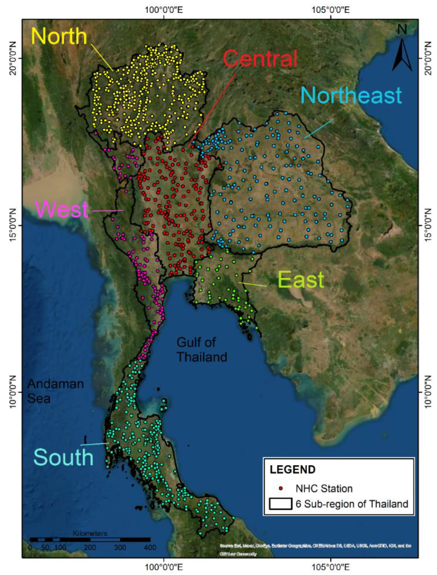
Figure 2.
Spatial distribution of a 24-hr accumulated rainfall on the target date along with its associated synoptic weather chart at 00UTC as summarized in Table 1.
Figure 2.
Spatial distribution of a 24-hr accumulated rainfall on the target date along with its associated synoptic weather chart at 00UTC as summarized in Table 1.
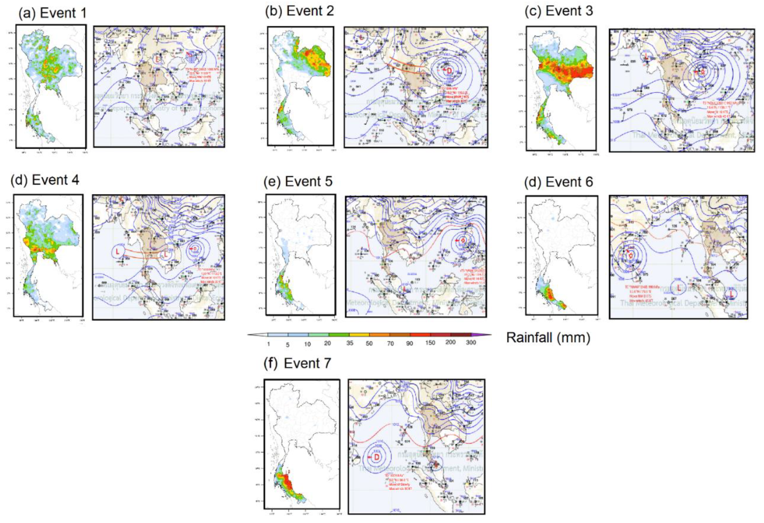
Figure 3.
Modeling domains of this study: (a) 3-nested WRF domains with (b) a single ROMS domain.
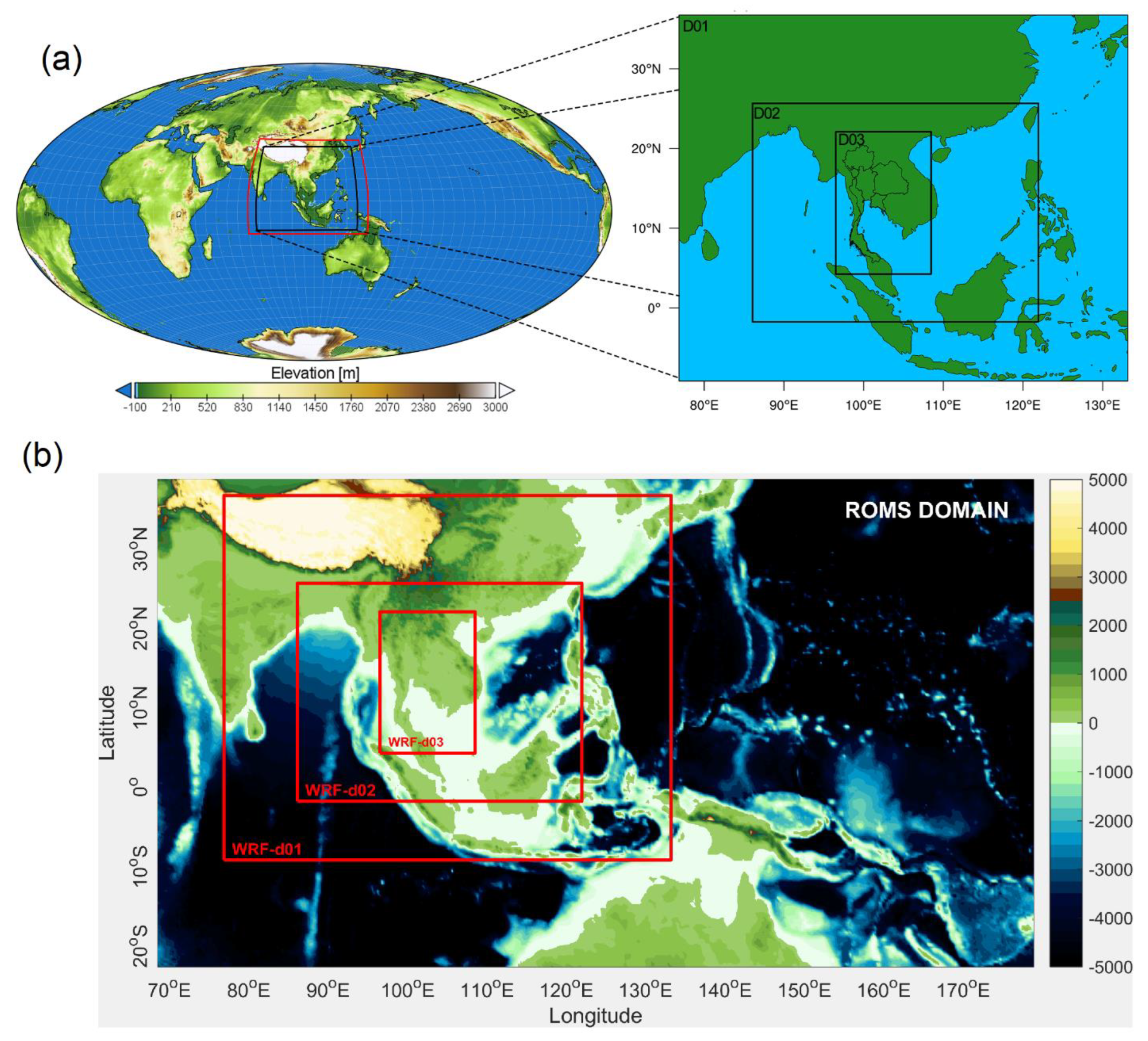
Figure 4.
POD of rainfall forecast with different MP and CU combinations.
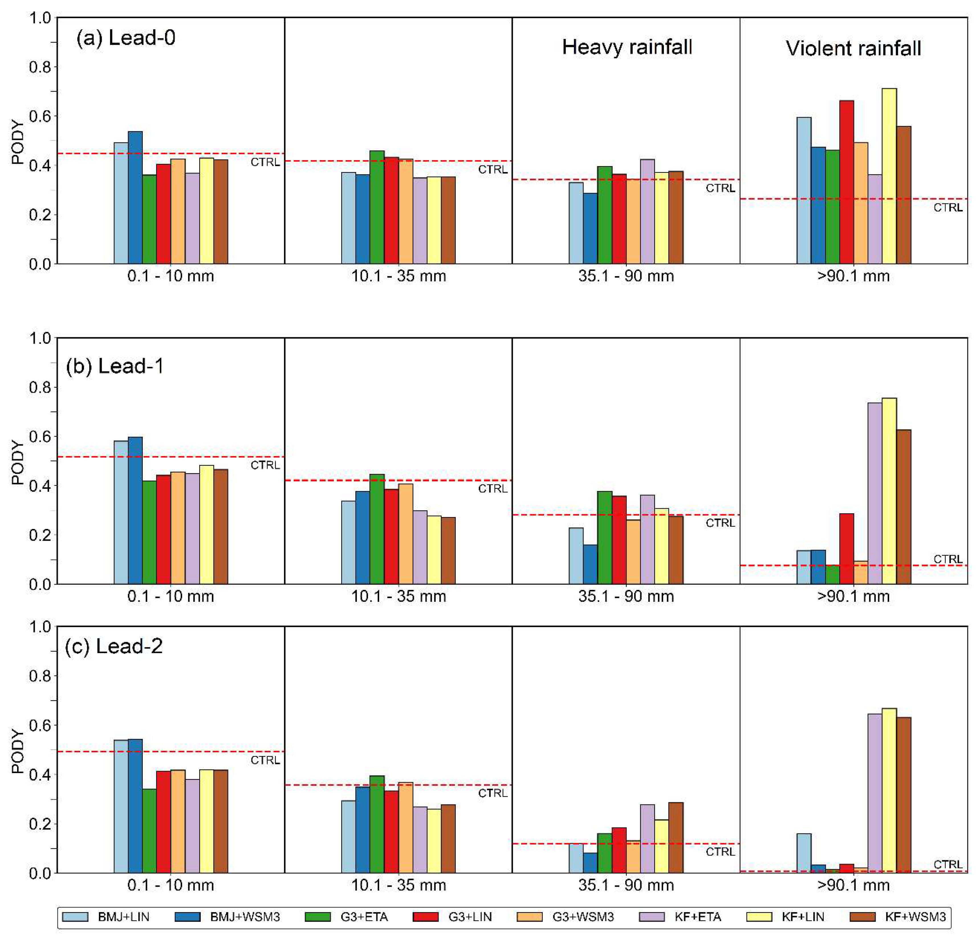
Figure 5.
Same as Figure 4, but for FAR.
Figure 5.
Same as Figure 4, but for FAR.
Figure 6.
Same as Figure 4, but for CSI.
Figure 6.
Same as Figure 4, but for CSI.

Table 1.
Selected heavy rainfall events in Thailand associated with atmospheric disturbed conditions in the 2020 and experimental designs for model integration with three different lead-times (Lead-0, 1, and 2).
Table 1.
Selected heavy rainfall events in Thailand associated with atmospheric disturbed conditions in the 2020 and experimental designs for model integration with three different lead-times (Lead-0, 1, and 2).
| Event No. |
Heay rainfall event (target date)* | During storm | Model initial date at 00 UTC | ||
|---|---|---|---|---|---|
| Lead-0 (24 hrs) |
Lead-1 (48 hrs) |
Lead-2 (72 hrs) |
|||
| Event 1 | 14 June | TD Nuri | 14 Jun. | 13 Jun. | 12 Jun. |
| Event 2 | 01 August | TD Sinlaku | 01 Aug. | 31 Jul. | 30 Jul. |
| Event 3 | 18 September | TS Noul | 18 Sep. | 17 Sep. | 16 Sep. |
| Event 4 | 16 October | TD | 16 Oct. | 15 Oct. | 14 Oct. |
| Event 5 | 12 November | sTS Vamco | 12 Nov. | 11 Nov. | 10 Nov. |
| Event 6 | 26 November | TC Nivar | 26 Nov. | 25 Nov. | 24 Nov. |
| Event 7 | 01 December | TD | 01 Dec. | 30 Nov. | 29 Nov. |
TD: Tropical depression, TS: Tropical storm, sTS: Severe tropical storm, and TC: Tropical cyclone. * The target date refers to the date when the storm approaches or is in close proximity to Thailand, resulting in significant rainfall.
Table 2.
Selected heavy rainfall events in Thailand associated with tropical storms and three model initial date/time runs for model validation.
Table 2.
Selected heavy rainfall events in Thailand associated with tropical storms and three model initial date/time runs for model validation.
| EXP | CU | Reference | MP | Reference |
|---|---|---|---|---|
| CTL* | BMJ | Janjic [51] | ETA | Zhao and Carr [52] |
| EXP-01 | BMJ | LIN | Chen and Sun [53] | |
| EXP-02 | BMJ | WSM3 | Hong, et al. [54] | |
| EXP-03 | G3 | Grell and Dévényi [55] | ETA | |
| EXP-04 | G3 | LIN | ||
| EXP-05 | G3 | WSM3 | ||
| EXP-06 | KF | Kain [56] | ETA | |
| EXP-07 | KF | LIN | ||
| EXP-08 | KF | WSM3 |
*CTL: Control run experiment.
Table 3.
Summary of CU and MP used in this study [61].
Table 3.
Summary of CU and MP used in this study [61].
| CU Scheme | Moisture Tendencies |
Momentum Tendencies |
Shallow Convection |
|---|---|---|---|
| BMJ | - | No | Yes |
| G3 | Qc, Qi | No | Yes |
| KF | Qc, Qr, Qi, Qs | No | Yes |
| MP Scheme | Mass Variables | ||
| ETA | Qc, Qr, Qs (Qt*) | ||
| LIN | Qc, Qr, Qi, Qs, Qg | ||
| WSM3 | Qc, Qr | ||
Qc: cloud, Qi: ice, Qr: mixing ratio for rain, Qs: snow, Qg: graupel; Qt*: total water mixing ratio tendency.
Disclaimer/Publisher’s Note: The statements, opinions and data contained in all publications are solely those of the individual author(s) and contributor(s) and not of MDPI and/or the editor(s). MDPI and/or the editor(s) disclaim responsibility for any injury to people or property resulting from any ideas, methods, instructions or products referred to in the content. |
© 2023 by the authors. Licensee MDPI, Basel, Switzerland. This article is an open access article distributed under the terms and conditions of the Creative Commons Attribution (CC BY) license (http://creativecommons.org/licenses/by/4.0/).
Copyright: This open access article is published under a Creative Commons CC BY 4.0 license, which permit the free download, distribution, and reuse, provided that the author and preprint are cited in any reuse.


