
Submitted:
13 July 2023
Posted:
17 July 2023
You are already at the latest version
Abstract
Hyperspectral image and LiDAR image fusion plays a crucial role in remote sensing by capturing spatial relationships and modeling semantic information for accurate classification and recognition. However, existing methods, like Graph Convolutional Networks (GCNs), face challenges in constructing effective graph structures due to variations in local semantic information and limited receptiveness to large-scale contextual structures. To overcome these limitations, we proposed a invariant attribute-driven binary bi-branch classification (IABC) method which is a unified network that combines binary Convolutional Neural Network (CNN) and GCN with invariant attributes. Our approach utilizes a joint detection framework that can simultaneously learn features from small-scale regular regions and large-scale irregular regions, resulting in an enhanced structured representation of HSI and LiDAR images in the spectral-spatial domain. This approach not only improves the accuracy of classification and recognition but also reduces storage requirements and enables real-time decision-making, which is crucial for effectively processing large-scale remote sensing data. Extensive experiments demonstrates the superior performance of our proposed method in hyperspectral image analysis tasks. The combination of CNNs and GCNs allows for accurate modeling of spatial relationships and effective construction of graph structures. Furthermore, the integration of binary quantization enhances computational efficiency, enabling real-time processing of large-scale data. Therefore, our approach presents a promising opportunity for advancing remote sensing applications using deep learning techniques.
Keywords:
Invariant Graph Convolutional Network (GCN)
; Convolutional Neural Network (CNN)
; Binary quantization
; Hyperspectral image (HSI) classification
1. Introduction
Geospatial classification plays a pivotal role in diverse applications such as Earth observation, environmental science, and forest management. Sensor technology advancements have provided multiple data sources to support classification tasks. Among these sources, hyperspectral imagery (HSI) stands out with its hundreds of spectral bands, offering detailed information about land cover. However, its passive imaging mode makes it vulnerable to influence from cloudy weather conditions and difficult to distinguish objects with similar spectral reflectance. In contrast, the active acquisition of light detection and ranging (LiDAR) data is less affected by weather conditions. LiDAR data enables the capture of elevation information, which aids in evaluating the size and shape of specific objects. Currently, there is a growing interest in utilizing a combination of HSI and LiDAR data for accurate land cover classification. Various cooperative models have been studied to provide comprehensive explanations for the study area.
In the past few decades, numerous machine learning-based classifiers have been developed for the fusion classification tasks of HSI and LiDAR. Among these classifiers, Convolutional Neural Networks (CNNs) have emerged as the most commonly used tool for extracting spectral-spatial features from HSI and LiDAR images. Different variants of CNNs, including 1D-CNNs, 2D-CNNs, and 3D-CNNs, have been proposed to enhance the learning ability of spectral-spatial features. In terms of spectral learning, previous studies such as Hu et al. [1] utilized 1D CNNs to extract spectral features and classify HSIs by providing the pixel vector of available samples as input to the models. For spatial learning, Chen et al. [2] introduced a 2D CNN-based framework for hyperspectral image classification. While satisfactory results were achieved through spectral-spatial learning using 1D and 2D CNNs, there was a need to effectively combine the spectral and spatial information in HSIs to achieve more robust abstraction. This led to the incorporation of 3D CNNs in HSI processing frameworks. Chen et al. [2] introduced a basic 3D CNN for HSI classification that outperformed existing benchmarks. Similarly, Zhong et al. [3] proposed a 3D framework that sequentially extracted spectral and spatial features from HSIs for classification. Another example is the work of Ying et al. [4], who proposed a 3D-CNN that utilizes three-dimensional convolution to learn spectral-spatial features.
Additionally, the verification of combining the advantages of different structural networks to enhance feature information extraction and improve classification accuracy has also been validated. Xu et al. [5] introduced a two-branch CNN for spectral and spatial learning, employing 1D and 2D CNNs in parallel for HSI and LiDAR classification. Yang et al. [6] presented a dual-channel CNN (TCCNN) that integrates one-dimensional and two-dimensional convolution branches to extract both spectral and spatial features. Furthermore, Chen et al. [7] proposed a multichannel CNN (MCCNN) with an additional 3D convolution branch based on TCCNN. However, their experiments indicated a limited improvement from the inclusion of extra branches, potentially due to suboptimal compatibility between different network branches. To address this issue, Hao et al. [8] proposed adaptive learning of fusion weights for different categories to balance the features extracted by different branches.
Graph Convolutional Networks (GCNs) are popular and emerging network architectures that effectively handle graph-structured data by modeling relationships between samples (vertices). Therefore, GCNs can naturally be used to simulate remote spatial relationships in hyperspectral images, which are not considered in CNNs. Shahraki and Prasad [9] combined 1D CNNs and GCNs for HS image classification. Wan et al. [10,11] performed super-pixel segmentation technology on the hyperspectral image which allows for the adjacency matrix to be updated dynamically with network iteration. Qin et al. [12] developed a new method of constructing graphs to second-order versions based on combining spatial and spectral neighborhoods simultaneously, and improved the ability to classify remote sensing images. Hong et al. proposed miniGCN, adopting mini-batch learning to train GCN with a fixed scale to reduce computational costs and improve classification accuracy. However, GCNs have some potential limitations in the following aspects and are less used in multimodal data classification in the remote sensing community.
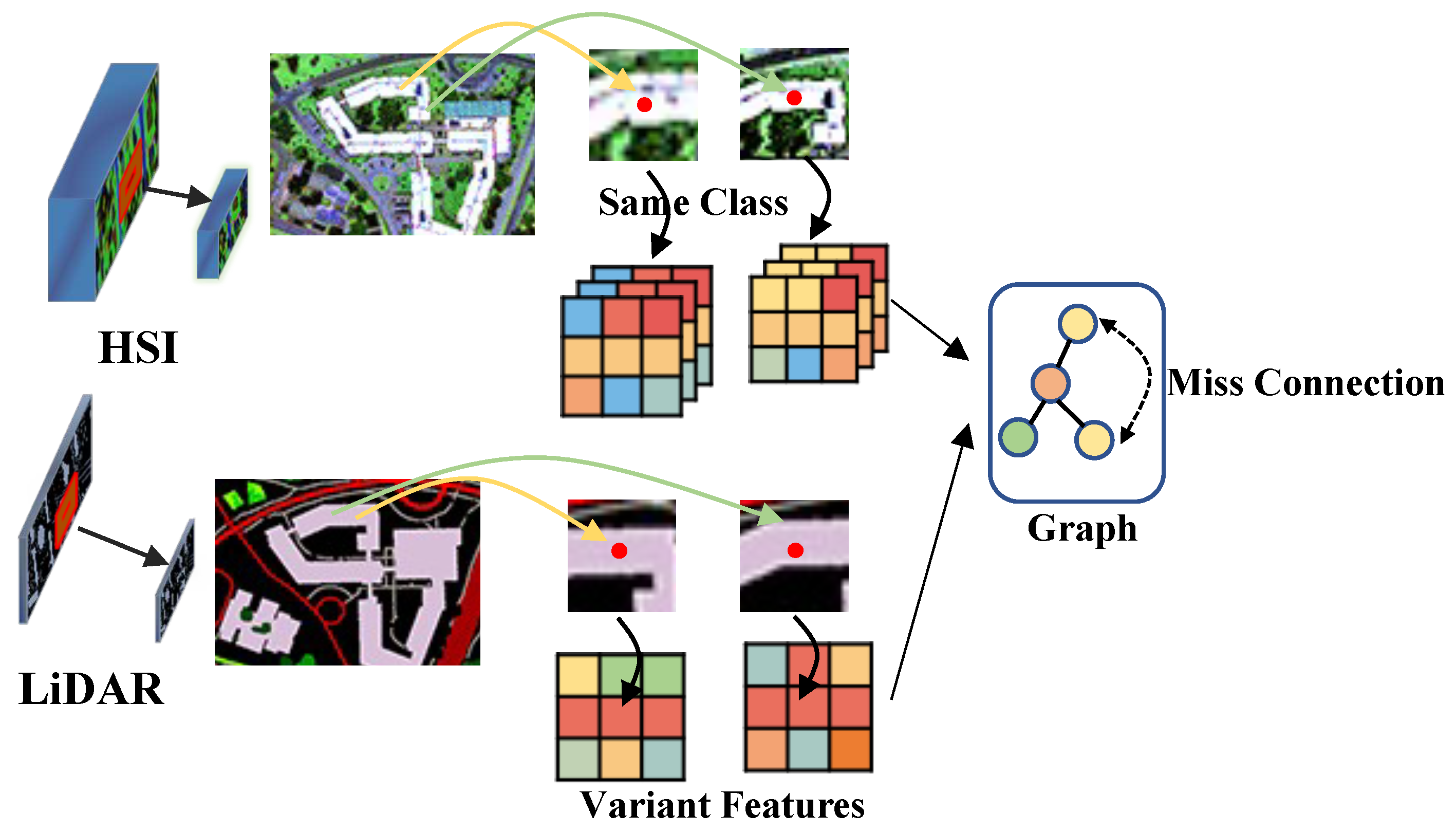
As shown in Figure 1, Variations in the local semantic information around target pixels, such as scene composition and relative positions between objects, lead to significant feature variations when modeling spatial information. This results in inaccurate graph structure construction in GCN networks, where effective connections cannot be established between pixels of the same class in spatial contexts. Therefore, we propose an approach to solve this problem by extracting invariant features locally from hyperspectral images in both spatial and frequency domains using the invariant attribute configuration method. While CNNs can learn local spectral spatial features at the pixel level, their receptive fields are typically limited to small square windows, making it difficult to capture large-scale contextual structures in images. We propose to integrate CNNs and GCNs into a single network, where the CNN branch learns pixel-level features within small regular regions, and the GCN branch models generate semantic-level features in irregular regions of the image. By doing so, we combine the advantages of both CNNs and GCNs. Additionally, due to the imaging mechanism and high-dimensional characteristics of hyperspectral bands, hyperspectral data has a lower spatial resolution. Rich spectral information provides details about material composition, and spatial information complements spectral information, enhancing object recognition capabilities. Henceforth, Our CNN network is designed as a binary-quantized network to address computational challenges and enhance the inference speed of the CNN model. Binary quantization offers several advantages in the field of remote sensing, including a significant reduction in storage requirements as binary values consume less memory compared to floating-point values. Moreover, by adopting binary quantization, we are able to alleviate resource constraints and enable real-time decision-making capabilities, which are crucial for efficiently processing large-scale data in remote sensing applications.
- We systematically analyze the sensitivity of CNN and GCN neural networks to variations such as rotation, translation, and semantic information. To the best of our knowledge, this is the first investigation in the community to explore the importance of spatial invariance on CNN and GCN networks. By extracting invariant features, we address the problem of feature variations caused by local semantic changes in spatial information modeling, thereby improving the accuracy of graph structure construction in the GCN network.
- By leveraging the advantages of both CNN and GCN, our proposed joint detection framework can simultaneously learn features from small-scale regular regions and large-scale irregular regions, resulting in an enhanced structured representation of HSI and LiDAR images in the spectral-spatial domain. This improvement contributes to an overall enhancement in the classification accuracy of the model.
- To address the challenges posed by the high-dimensional nature of hyperspectral data and computational resource limitations, we introduce a lightweight binary CNN architecture that significantly reduces the number of parameters and computational requirements while still maintaining a high level of classification performance.
Figure 1.
The graph structure construction is influenced by feature variations in the same class field.
Figure 1.
The graph structure construction is influenced by feature variations in the same class field.
The structure of the paper is outlined as follows. Section 2 reviews the existing literature on multimodal classification and network compression. Section 3 elaborates on the proposed IABC approach. The experimental results and comprehensive analysis of the method are presented in Section 4. Finally, Section 5 and Section 6 discuss the implications and conclude the findings of our method, respectively.
2. Related Work
In this section, we briefly review two key aspects relevant to our work: multimodal classification and network compression.
2.1. Multimodal Classification
Multimodal fusion algorithms commonly employ pixels or features as the fundamental units for image fusion, which can be categorized into three stages of data fusion: 1) early fusion, 2) inter-layer fusion, and 3) late fusion [13,14,15]. Additionally, multimodal image fusion can be further classified based on existing image classification algorithms into 1) traditional machine learning algorithms, 2) classical deep learning algorithms, and 3) Transformer algorithms. Traditional machine learning algorithms include SVM [16] and KNN [17], while classical deep learning algorithms include CNN and RNN [18]. Fusion based on convolutional neural networks can yield compact modal representations. For instance, Hong et al. [19] proposed a deep encoder-decoder network architecture for hyperspectral and LiDAR data classification. Liu et al. [20] introduced a novel heterogeneous deep network using both CNN and GCN branches to learn features from small-scale regular regions and large-scale irregular regions. Fusion frameworks based on Transformers can generate desirable results, and Roy et al. [21] developed a novel multimodal fusion transformer network that integrates external classification markers from other multimodal data into the transformer encoders, leading to improved generalization performance. Although traditional methods are easy to implement, they may suffer from classification errors and low-level features, which can potentially degrade overall accuracy.
In this study, we present a novel algorithm for multi-modal remote sensing image classification using a miniature convolutional network. Our approach incorporates a joint feature extraction framework that combines a miniature convolutional network and a two-dimensional convolutional neural network. By leveraging this framework, we aim to enhance the extraction of high-level information representations to overcome the limitations posed by the weak robustness of feature information and single-feature information, ultimately improving the classification performance.
2.2. Network Compression
Public remote sensing image datasets are typically smaller than natural datasets consisting of millions of samples, resulting in a significant amount of redundancy in parameters and network structures. Moreover, the high computational cost and memory usage associated with over-parameterization hinder the application of remote sensing techniques in resource- and time-sensitive scenarios or limited hardware endpoints, such as real-time inference systems on satellites’ onboard processing platforms, mobile platforms, and embedded devices. In this context, various network compression techniques have been proposed, including compact network design [22], tensor decomposition, network pruning, quantization, and knowledge distillation. Han et al. [23] describes a method to reduce the storage and computation required by neural networks by an order of magnitude without affecting their accuracy by learning only the important connections. Li et al. [24] report an architecture named random sketch learning, or Rosler, for computationally efficient tiny artificial intelligence
In this study, binary quantization operations were applied to the input and output layers of the multilayer perceptron in the spectral attention mechanism, as well as to the convolutional layers and each downsampling layer in the spatial attention mechanism within the network structure. Moreover, performing quantization operations at different levels on the weights and activations is beneficial for improving the model’s performance accuracy.
3. Proposed Method
3.1. Invariant Attribute Consistency Fusion
As shown in Figure 2, the Invariant Attribute Consistency Fusion includes two parts: Invariant Attribute Extraction (IAE) and Spatial-Consistency Fusion (SCF). Extracting invariant attribute features can counteract local semantic changes caused by Pixel rotation and movement or local regional composition changes. We utilize the Invariant Attribute Profiles (IAPs) [25] for feature extraction to enhance the diversity of features and model the invariant behaviors in multimodal data. This approach generates robust feature extraction for various semantic changes in multimodal remote sensing data. Firstly, the multimodal remote sensing images are filtered using isotropic filters to obtain more robust convolutional features, referred to as Robustness Convolutional Features (RCFs). The RCFs are expressed as:
where, H represents the HSI, L represents the LiDAR image, denotes the RCF extracted from the k-th band of the multimodal remote sensing image. is the input remote sensing image, represents isotropic filtering, achieved by convolving with , thereby extracting spatially invariant features from local space. Additionally, robustness is enhanced by utilizing superpixel segmentation methods to enhance the spatial invariance of the features based on object semantics, such as edges, shapes, and their invariance.
where represents the segmentation of superpixels. Additionally, and represent the representations of spatially invariant attribute features for the HSI and LiDAR images, respectively. To achieve invariance to translation and rotation in the frequency domain, we construct a continuous histogram of oriented gradients in Fourier polar coordinates. By utilizing the Fourier-based continuous Histogram of Oriented Gradients (HOG), we ensure invariant feature extraction in polar coordinates. This approach accurately captures rotation behaviors at any angle. Therefore, by mapping the translation or rotation of image blocks in Fourier polar coordinates, discrete attribute features are transformed into continuous contours. Consequently, we obtain Frequency Invariant Features (FIF) in the frequency domain.
By utilizing the extracted spatially invariant features, and , along with the frequency invariant features, and , we obtain the joint invariant attribute features, denoted as :
Spatial-Consistency Fusion is designed to enhance the consistency of similar features in the observed area’s terrain feature information. We employ the Generalized Graph-Based Fusion (GGF) method [26] to jointly extract consistent feature information of different modalities’ invariant attributes.
where , , and represent HSI, invariant features of HSI, and invariant features of LiDAR, respectively. The HSI is specifically used to capture the consistency information in the spectral dimension. is the fusion result. W denotes the transformation matrix used to reduce the dimensionality of the feature maps, fuse the feature information, preserve local neighborhood information, and detect manifolds embedded in a high-dimensional feature space.
Initially, a graph structure is constructed to describe the correlation between spatial sample points and obtain the edge consistency information of the graph structure for different modalities:
where , , and are defined as the edges of the graph structures , and , respectively. They are obtained through the k-nearest neighbors (k-NN) method. When two sample points i and j are close in distance (strong correlation), . When the distance between two sample points is large (weak correlation), . The likelihood of a data point having similar features to its nearest neighbor is greater than with those points that are far away. Therefore, it is necessary to add a distance constraint when calculating graph edges. This can be defined as:
where is the pairwise distance matrix between the individual data points in . In , the final graph structure is determined by applying the k-nearest neighbor approach to identify the edge . Then, , the diagonal matrix, is computed based on . Subsequently, the Laplacian matrix is obtained through this process:
By combining the known feature information , the Laplacian matrix , and the diagonal matrix , we can use the following generalized eigenvalue calculation formula to obtain different eigenvalues and their corresponding eigenvectors :
where, denotes the transpose matrix of , represents the eigenvalue, with indicating the number of eigenvalues. Since each eigenvector has its own unique eigenvalue, we can obtain . Finally, based on all the eigenvectors, we can obtain the desired transformation matrix :
where, represents an eigenvector corresponding to the i-th eigenvalue.
3.2. Bi-Branch Joint Classification
The GCN and CNN are architectural designs used to extract distinct representations of salient information from multimodal remote-sensing images. The CNN specializes in capturing intricate spatial features, while the GCN excels at extracting abundant spectral feature information from multimodal remote sensing images by utilizing spectral vectors as input. Additionally, the GCN can simulate the topological relationships between samples in graph-structured data. We design a bi-branch joint classification combining the advantages of the GCN and CCN to offer various feature diversity.
Traditional GCNs effectively model the relationships between samples to simulate long-range spatial relationships in remote sensing images. However, inputting all samples into the network at once leads to significant memory overhead. To address these issues, the Mini Graph Convolutional Network (MiniGCN) [27] is introduced to find robust locally optimal feature information by utilizing a sampler for small-sample sampling, dividing the original input graph-structured data into multiple subgraphs. The graph-structured multimodal fused image data is input into the MiniGCN in a matrix form for training. During the training process, the input data is processed and features are extracted and outputted in mini-batches. The classification output can be represented by the following equation:
where, can be translated as follows: is the adjacency matrix of spatial-frequency invariant attribute features , and is the modified adjacency matrix. represents the weight of the l-th layer in the graph convolutional network. denotes the diagonal matrix of . represents the ReLU non-linear activation function. represents the feature output of the l-th layer in the graph convolutional network during the feature extraction process. When , corresponds to the original input features. represents the feature output of the -th layer in the graph convolutional network, which serves as the final output spectral features.
In addition, we utilize a simple CNN structure [28] which can be defined as:
Here, the base structure includes the convolutional layer, batch normalization layer, max-pooling layer, and ReLU layer. Therefore, we use adaptive coefficients to combine the detection results of the two networks, which can be represented as:
where, represents the classification head function, while and refer to the features extracted by the GCN and the CNN, respectively. The and are learnable parameters of the network to balance the weight of the bi-branch results.
3.3. Binary Quantization
To ensure the retention of information and minimize information loss during forward propagation, we propose the utilization of Libra Parameter Binarization (Libra-PB) [29], which incorporates both quantization error and information loss. During forward propagation, the full-precision weights are initially adjusted by subtracting the mean of the weights. This adjustment aims to distribute the quantized values uniformly and normalize the weight, thereby enhancing training stability and mitigating any negative effects caused by weight magnitude. The resultant standardized balanced weight, denoted as , can be obtained through the following operations:
In the above equation, represents the standard deviation, while is the mean of the full-precision weights. The objective of network binarization is to represent the floating-point weights and/or activations using only 1-bit. Generally, the quantization of weights and activations can be defined as:
Here, and a represent the floating-point parameters of weights and activations. The function is commonly employed to obtain binary values, and it can be computed as:
s is an integer parameter used for expanding the representation ability of binary weights. It can be calculated as:
Here, n represents the dimension of the vector and denotes its L1-norm. The main operations in the forward propagation of binary CNN, involving quantized weights and activations , can be expressed as:
During backward propagation, due to the discontinuity introduced by binarization, gradient approximation becomes necessary. The approximation can be formulated as:
where, represents the loss function, denotes the approximation of the sign function, and is its derivative. In our paper, we use the following approximation function:
3.4. Loss Function
The output of , and passing a softmax classify layer to predict the probability distribution. The overall network is trained by the following loss function:
Here, refers to the label of the dataset, and denotes the cumulative L2 norm, utilized for determining the weights across all network layers. This approach is employed to address the issue of overfitting which arises when there is an excessive number of model parameters.
3.5. Experimental Setup
Data Description: (1) Houston2013 Data: Experiments were carried out using hyperspectral imaging (HSI) and digital surface model (DSM) data that were obtained in June 2012 over the University of Houston campus and the adjacent urban area. The HSI data consisted of 144 spectral bands and covered a wavelength range from 380 to 1050 nm, with a spatial resolution of 2.5 m that was consistent with the DSM data. The entire dataset covered an area of pixels and included 15 classes of natural and artificial objects, which were determined through photo interpretation by the DFTC. The LiDAR data was collected at an average sensor height of 2000 feet, while the HSI was collected at an average height of 5500 feet. The scene contained various natural objects such as water, soil, trees, and grass, as well as artificial objects such as parking lots, railways, highways, and roads. Table 1 reports the land cover classes and the corresponding number of training and testing samples.
(2) Trento Data: It comprises one HSI with 63 spectral bands and one LiDAR data, captured in a rural area located in southern Trento, Italy. The HSI was obtained through the AISA Eagle sensor, while the corresponding LiDAR data was collected using the Optech Airborne Laser Terrain Mapper (ALTM) 3100EA sensor. Both datasets are of size pixels with a spatial resolution of 1 m, while the wavelength range of HSI is from 0.42 to 0.99 m. This particular data set consists of a total of 30,214 ground-truth samples, with research conducted on 6 distinguishable category labels. Table 1 reports the land cover classes and the corresponding number of training and testing samples.
Evaluation Metrics: To comprehensively evaluate the performance of multimodal remote sensing image classification algorithms, this article analyzes and compares various algorithms based on their classification prediction maps and accuracy. While the classification prediction map is subject to a certain degree of subjectivity and may not accurately measure the impact of an algorithm on classification performance, this study employs quantitative evaluation metrics such as overall accuracy (OA), average accuracy (AA), and Kappa coefficient to better measure and compare the performance of different algorithms. A higher value of any of these three indicators represents higher classification accuracy and overall better performance of the algorithm. Among these three evaluation metrics, overall accuracy (OA) refers to the ratio of correctly classified test samples to the total number of test samples. Average accuracy (AA) refers to the ratio of correctly classified test samples to the total number of test samples in a specific category. The kappa coefficient is expressed as:
where N represents the total number of sample points, represents the values in the diagonal of the confusion matrix obtained after classification, and and represent the total number of samples in a certain category as well as the number of samples that have been correctly classified in this category, respectively. Furthermore, we employ Bit-Operations (BOPs) count [30] and parameters as metrics to evaluate the compression performance. The BOPs for convolution can be determined using the following equation:
Here, , , and represent the height, width, and number of channels of the output feature map of the layer, respectively. and indicate the weight and activation bit-widths of the layer. and correspond to the size of the convolution kernel. The parameters (params) are defined as:
Implementation Details: Our proposed approach is implemented in Python with TensorFlow and trained on 1 RTX 3090 card. All the networks considered in this paper are implemented using the TensorFlow platform. During this process, we set the batch size to 32, utilize Adam with an initial learning rate of 0.005, and perform a total of 200 epochs. The current learning rate is adjusted using an exponential learning rate strategy, where the learning rate is multiplied by every 50 epochs. Additionally, weight regularization is applied using the L2 norm to stabilize network training and reduce overfitting.
3.6. Ablation Study
An ablation study is conducted to demonstrate the validity of the proposed components by evaluating several variants of the IABC on HSI and LiDAR datasets.
Invariant Attribute Consistency Fusion:Table 2 discusses the impact of using IACF (IAE structure and SCA Fusion) on CNN and GNN networks in remote sensing image classification tasks, as well as the comparison between multi-modal and single-modal HSI and LiDAR data. The Houston2013 dataset is used for evaluation, and metrics such as OA, AA, and Kappa coefficient are used to measure classification performance. Firstly, the experimental results for HSI data show that both GCN and CNN networks achieve a certain level of accuracy in classification but differ in precision. The introduction of the IAE structure improves classification performance, increasing OA and AA from 79.04% and 81.16% to 91.15% and 91.78% respectively. This indicates the effectiveness of the IAE structure in improving the accuracy of remote sensing image classification. Secondly, the experimental results for LiDAR data demonstrate a lower classification accuracy when using GCN or CNN networks alone. However, the introduction of the IAE structure significantly improves classification performance. For example, OA increases from 22.74% to 41.81%. This confirms the effectiveness of the IAE structure in processing LiDAR data. Lastly, fusion experiments are conducted with HSI and LiDAR data. The results show that fusing HSI and LiDAR data further improves classification performance. When combining the CNN network, IAE structure, and SCA fusion, the OA performance reaches 91.88%, an increase of 2.43%.
Similarly, on the Trento dataset, as shown in Table 3, the same conclusions were obtained. In the case of HSI data, when only GCN or CNN was used, the overall accuracy (OA) was 83.96% and 96.06%, respectively. However, when the IAE structure was introduced for invariant feature extraction, the OA accuracy improved to 95.34% (an increase of 11.38%) and 96.93% (an increase of 0.87%) for GCN and CNN, respectively. This indicates that the extraction of spatially invariant attributes can reduce the heterogeneity in extracting pixel features of the same class by CNN and GNN networks, enhancing the discriminative ability for the same class. Moreover, the extraction of invariant attributes has a more significant effect on improving the classification accuracy of the GCN network. When classifying LiDAR data, due to the characteristics of LiDAR data, the performance is relatively low, with only the GCN network achieving an OA of 48.31%. Introducing IAE can improve the GCN network OA by 11.94%. However, introducing IAE to the CNN network instead results in a decrease in classification performance from 90.81% to 68.81%. This might be due to the large size of areas with the same class in the Trento dataset, resulting in minimal elevation changes in the LiDAR images over a considerable area, leading to similar invariant attributes for different classes and interfering with the CNN network’s ability to extract and discriminate local information. This situation can be alleviated when using multimodal data (HSI+LiDAR) for classification. Considering the information from both the HSI and LiDAR, better performance can be observed. Particularly, the best classification performance (OA 98.05%) was achieved when CNN introduced the IAE structure and SCA fusion.
This further demonstrates that SCA fusion can enhance the classification accuracy of the CNN network. In conclusion, this experiment proves that the introduction of the IAE structure significantly improves the classification performance of CNN and GNN networks in remote sensing image classification tasks. Additionally, SCA enhances the classification performance of the CNN network. Furthermore, the fusion of multi-modal data can further improve classification accuracy.
Bi-branch Joint Classification: To analyze the performance of the bi-branch joint network for classification, we compare the different networks in the two datasets in Figure 5. Regarding the Houston2013 dataset, the results showed that CNN achieved an OA of 91.88%, an AA of 92.60%, and a of 91.97%. GCN achieved an OA of 92.60%, an AA of 93.20%, and a of 91.97%. On the other hand, the Joint method achieved an OA of 92.78%, an AA of 93.29%, and a of 92.15%. For the Trento dataset, similar classification experiments were conducted using CNN, GCN, and the Joint method. The results showed that CNN achieved high OA (98.05%) and AA (95.18%), as well as a high (97.73%). GCN obtained lower OA (97.66%) and AA (96.38%), as well as a lower (96.87%). In contrast, the Joint method achieved the best classification results on the Trento dataset, with an OA of 98.14%, an AA of 97.03%, and a of 97.50%. The experimental results demonstrate that using the bi-branch joint network can combine the advantages of CNN and GCN networks, resulting in excellent classification performance in remote sensing image land classification tasks.
Binary Quantization: With the application of binary quantization, we can effectively address resource limitations and enable real-time decision-making capabilities in the context of processing large-scale data in remote sensing applications. To analyze the performance differences, we conducted a comparative study on classification accuracy and computational resources using different quantization strategies on the IABC network. The results are presented in Table 4, where 32w and 32a denote the full precision of the weight and activation while 1w and 1a represent the binary quantization of the weight and activation. The binary quantization module achieved OA accuracies of 98.14%, 98.16%, 85.33%, and 83.44% at different computational levels. Notably, the difference in OA accuracy between the 1w32a quantization level and the full precision network is relatively small. Additionally, for the CNN network at the 1w32a quantization level, the parameter count is 32.675KB, which accounts for only 3% of the parameter count of the full precision network. Likewise, the BOPs are approximately 3% of the BOPs in the full precision network. It is observed that the accuracy of the classification model decreases as the number of quantization bits decreases. This decrease may be attributed to the reduced number of model parameters, leading to the loss of certain important layer information and consequently resulting in a decline in accuracy. It is observed that the binary quantization of the activations has a significantly bad impact on the classification accuracy, and the OA decreases by 12.81% compared with the full-precision network and 12.53% compared with the quantization weight only (1w32a). Particularly, when using the 1w1a network exclusively, the impact is notably significant, with the resulting 14.7% accuracy reduction compared to a full-precision network. Hence, we only consider the binary quantization of the weights 1w32a in our experiment.
3.7. Quantitative Comparison with the State-of-the-art Classification Network
To validate the effectiveness of the proposed IABC, we compare the experimental results of the IABC on both HSI and LiDAR datasets with those of other competitive classifiers MDL_RS_FC [28], EndNet [31], RNN [18], CALC [32], ViT [33] and MFT [21]. We optimize the parameters of all the compared methods on the same server as described in the original article. Additionally, for a fair comparison, we use identical training and testing samples. Data augmentation techniques are commonly employed to prevent model overfitting and enhance classification accuracy. However, conventional image processing-based methods, such as flipping and rotation, can be easily learned by the model. To ensure a fair comparison with other approaches, our proposed IABC network abstains from utilizing any data augmentation operations. Table 6 and Table 7 showcase the objective classification outcomes of various methods on two experimental datasets. The most favorable results in each row are highlighted in red. It can be seen that the proposed IABC is superior to other methods. Taking the Houston2013 as an example, IABC provides approximately 7.67%, 7.6%, 20.32% 2.84%, 7.58% 3.03% OA improvements for MDL_RS_FC, Endnet, RNN, CALC, ViT, and MFT, respectively, and achieve the highest classification accuracy for seven of the 15 categories. RNN performs the worst with only 72.31% OA. Due to its designed cross-fusion strategy, the MDL_RS_FC method achieves better performance which is 84.96% OA because there is more sufficient information interaction in the feature fusion process. Conventional classifier EndNet by leveraging deep neural networks to enhance the ability of feature extraction for spectral and spatial features. Multiple types of feature extraction outperform single-type feature extraction. CALC method achieves the 89.79% OA ranking three which not only fully exploits and mines high-level semantic information and complementary information, but also increases adversarial training, which can effectively preserve detailed information in HSI and LiDAR data. Transformer-based methods ViT and MFT with their strong feature expression ability in high-level sequential abstract representation achieve higher accuracy than the traditional deep learning network (such as Endnet and MDL_RS_FC). In contrast, our IABC method achieves the best performance on OA, AA, and due to the joint use of spatial–spectral CNN and relation-augmented GCN features with invariant attributes enhancement. For the Trento dataset with higher spatial resolution and fewer feature categories, IABC provides approximately 10.40%, 7.58%, 2.24%, 0.56%, 2.2%, 0.35% improvements for MDL_RS_FC, Endnet, RNN, CALC, ViT, and MFT, respectively, and achieve the highest classification accuracy for three of the 6 categories. The performance of the RNN network on the Trento dataset is noticeably better compared with the result on the Houston2013 dataset while the MDL_RS_FC method performance is worse on the Trento dataset. It is proven that the generalization performance of these two methods is comparatively poor. The performance of other algorithms is consistent with the performance on the Houston2013 dataset.
The Figure 3 illustrates a range of visual data, including hyperspectral false-color images, LiDAR images, ground-truth plots, and classification maps, acquired using various methods on the two datasets. Each category is accompanied by its respective color scheme. Upon thorough evaluation and comparison, it is clear that the proposed methods yield superior results with significantly reduced noise compared to alternative approaches. Deep learning models excel in capturing the nonlinear relationship between input and output features, thanks to their remarkable ability to extract learnable features. Hence, all the methods generate relatively smooth classification maps, effectively distinguishing between different land-use and land-cover classes. Notably, Vit and MFT demonstrate their efficacy in classification by extracting high-level sequential abstract representations from images. Consequently, the classification maps exhibit better visual quality compared to fully connecting, CNN, and RNN networks. By enhancing neighboring spatial-spectral information and facilitating the effective transmission of relation-augmented information across layers, the proposed IABC method achieves highly desirable classification maps, particularly in terms of texture and edge details, surpassing CALC, ViT, and MFT.
4. Conclusion
In conclusion, our proposed unified network, combining CNNs and GCNs, presents a promising solution for hyperspectral image and LiDAR image fusion in remote sensing. By employing a joint detection framework, our approach effectively captures spatial relationships and models semantic information, resulting in an enhanced representation of HSI and LiDAR images in the spectral-spatial domain. Our method successfully addresses the limitations in constructing graph structures and showcases superior performance in hyperspectral image analysis. The utilization of CNNs and GCNs ensures accurate modeling of spatial relationships and the construction of effective graph structures. Moreover, the incorporation of binary quantization enhances computational efficiency, enabling real-time processing of large-scale data. Furthermore, our systematic analysis sheds light on the significance of spatial invariance and examines the sensitivity of CNN and GCN neural networks to variations, contributing to the overall understanding of the research community. Additionally, our introduction of a lightweight binary CNN architecture effectively tackles the challenges posed by high-dimensional hyperspectral data and computational limitations, while maintaining a high level of classification performance.
Overall, our approach offers a promising opportunity to advance remote sensing applications through the implementation of deep learning techniques. It significantly improves accuracy, reduces storage requirements, and enables real-time decision-making for large-scale remote sensing data processing.
Author Contributions
W.X. and J.Z. provided conceptualization; J.Z designed the methodology; J.Z performed the experiments and analyzed the result data; D.L. investigated related work; W.X. provided suggestions on paper revision; J.Z. and D.L. wrote the paper.
Funding
This work was supported in part by the National Natural Science Foundation of China under Grant 62071360.
Abbreviations
The following abbreviations are used in this manuscript:
| HSI | Hyperspectral image |
| CNN | Convolutional neural network |
| GCN | Graph convolution network |
| KNN | K nearest neighbors |
| OA | Overall accuracy |
| AA | Average accuracy |
| BOPs | Bit-Operations |
| Params | parameters |
References
- Hu, W.; Huang, Y.; Wei, L.; Zhang, F.; Li, H. Deep convolutional neural networks for hyperspectral image classification. J. Sensors 2015, 2015, 1–12. [Google Scholar] [CrossRef]
- Chen, Y.; Jiang, H.; Li, C.; Jia, X.; Ghamisi, P. Deep feature extraction and classification of hyperspectral images based on convolutional neural networks. IEEE Trans. Geosci. Remote Sens. 2016, 54, 6232–6251. [Google Scholar] [CrossRef]
- Zhong, Z.; Li, J.; Luo, Z.; Chapman, M. Spectral–spatial residual network for hyperspectral image classification: A 3-D deep learning framework. IEEE Trans. Geosci. Remote Sens. 2017, 56, 847–858. [Google Scholar] [CrossRef]
- Li, Y.; Zhang, H.; Shen, Q. Spectral–spatial classification of hyperspectral imagery with 3D convolutional neural network. Remote Sens. 2017, 9, 67. [Google Scholar] [CrossRef]
- Xu, X.; Li, W.; Ran, Q.; Du, Q.; Gao, L.; Zhang, B. Multisource remote sensing data classification based on convolutional neural network. IEEE Trans. Geosci. Remote Sens. 2017, 56, 937–949. [Google Scholar] [CrossRef]
- Yang, J.; Zhao, Y.Q.; Chan, J.C.W. Learning and transferring deep joint spectral–spatial features for hyperspectral classification. IEEE Trans. Geosci. Remote Sens. 2017, 55, 4729–4742. [Google Scholar] [CrossRef]
- Chen, C.; Zhang, J.J.; Zheng, C.H.; Yan, Q.; Xun, L.N. Classification of hyperspectral data using a multi-channel convolutional neural network. In Proceedings of the Intelligent Computing Methodologies: 14th International Conference, ICIC 2018, Wuhan, China, 2018, Proceedings, Part III 14. Springer, 2018, August 15-18; pp. 81–92.
- Hao, S.; Wang, W.; Ye, Y.; Nie, T.; Bruzzone, L. Two-stream deep architecture for hyperspectral image classification. IEEE Trans. Geosci. Remote Sens. 2017, 56, 2349–2361. [Google Scholar] [CrossRef]
- Shahraki, F.F.; Prasad, S. Graph convolutional neural networks for hyperspectral data classification. In Proceedings of the 2018 IEEE global conference on signal and information processing (GlobalSIP). IEEE; 2018; pp. 968–972. [Google Scholar]
- Wan, S.; Gong, C.; Zhong, P.; Pan, S.; Li, G.; Yang, J. Hyperspectral image classification with context-aware dynamic graph convolutional network. IEEE Trans. Geosci. Remote Sens. 2020, 59, 597–612. [Google Scholar] [CrossRef]
- Wan, S.; Gong, C.; Zhong, P.; Du, B.; Zhang, L.; Yang, J. Multiscale dynamic graph convolutional network for hyperspectral image classification. IEEE Trans. Geosci. Remote Sens. 2019, 58, 3162–3177. [Google Scholar] [CrossRef]
- Qin, A.; Shang, Z.; Tian, J.; Wang, Y.; Zhang, T.; Tang, Y.Y. Spectral–spatial graph convolutional networks for semisupervised hyperspectral image classification. IEEE Geosci. Remote Sens. Letters 2018, 16, 241–245. [Google Scholar] [CrossRef]
- Eigen, D.; Puhrsch, C.; Fergus, R. Depth Map Prediction from a Single Image using a Multi-Scale Deep Network. In Proceedings of the Advances in Neural Information Processing Systems (NIPS); Ghahramani, Z.; Welling, M.; Cortes, C.; Lawrence, N.; Weinberger, K., Eds. Curran Associates, Inc., Vol. 27. 2014. [Google Scholar]
- Dong, Y.; Liu, Q.; Du, B.; Zhang, L. Weighted feature fusion of convolutional neural network and graph attention network for hyperspectral image classification. IEEE Trans. Image Process. 2022, 31, 1559–1572. [Google Scholar] [CrossRef]
- Li, S.; Song, W.; Fang, L.; Chen, Y.; Ghamisi, P.; Benediktsson, J.A. Deep learning for hyperspectral image classification: An overview. IEEE Trans. Geosci. Remote Sens. 2019, 57, 6690–6709. [Google Scholar] [CrossRef]
- Melgani, F.; Bruzzone, L. Classification of hyperspectral remote sensing images with support vector machines. IEEE Trans. Geosci. Remote Sens. 2004, 42, 1778–1790. [Google Scholar] [CrossRef]
- Rasti, B.; Hong, D.; Hang, R.; Ghamisi, P.; Kang, X.; Chanussot, J.; Benediktsson, J.A. Feature extraction for hyperspectral imagery: The evolution from shallow to deep: Overview and toolbox. IEEE Geosci. Remote Sens. Mag. 2020, 8, 60–88. [Google Scholar] [CrossRef]
- Cho, K.; Van Merriënboer, B.; Bahdanau, D.; Bengio, Y. On the properties of neural machine translation: Encoder-decoder approaches. arXiv preprint arXiv:1409.1259 2014. arXiv:1409.1259 2014.
- Hong, D.; Gao, L.; Hang, R.; Zhang, B.; Chanussot, J. Deep encoder–decoder networks for classification of hyperspectral and LiDAR data. IEEE Geosci. Remote Sens. Lett. 2020, 19, 1–5. [Google Scholar] [CrossRef]
- Liu, Q.; Xiao, L.; Yang, J.; Wei, Z. CNN-enhanced graph convolutional network with pixel-and superpixel-level feature fusion for hyperspectral image classification. IEEE Trans. Geosci. Remote Sens. 2020, 59, 8657–8671. [Google Scholar] [CrossRef]
- Roy, S.K.; Deria, A.; Hong, D.; Rasti, B.; Plaza, A.; Chanussot, J. Multimodal fusion transformer for remote sensing image classification. IEEE Trans. Geosci. Remote Sens. 2023. [Google Scholar] [CrossRef]
- Zhang, Y.M.; Lee, C.C.; Hsieh, J.W.; Fan, K.C. CSL-YOLO: A new lightweight object detection system for edge computing. arXiv preprint arXiv:2107.04829 2021. arXiv:2107.04829 2021.
- Han, S.; Pool, J.; Tran, J.; Dally, W. Learning both weights and connections for efficient neural network. Advances in neural information processing systems (NIPS) 2015, 28. [Google Scholar]
- Li, B.; Chen, P.; Liu, H.; Guo, W.; Cao, X.; Du, J.; Zhao, C.; Zhang, J. Random sketch learning for deep neural networks in edge computing. Nat. Comput. Sci. 2021, 1, 221–228. [Google Scholar] [CrossRef]
- Hong, D.; Wu, X.; Ghamisi, P.; Chanussot, J.; Yokoya, N.; Zhu, X.X. Invariant attribute profiles: A spatial-frequency joint feature extractor for hyperspectral image classification. IEEE Trans. Geosci. Remote Sens. 2020, 58, 3791–3808. [Google Scholar] [CrossRef]
- Liao, W.; Pižurica, A.; Bellens, R.; Gautama, S.; Philips, W. Generalized graph-based fusion of hyperspectral and LiDAR data using morphological features. EEE Geosci. Remote Sens. Lett. 2014, 12, 552–556. [Google Scholar] [CrossRef]
- Hong, D.; Gao, L.; Yao, J.; Zhang, B.; Plaza, A.; Chanussot, J. Graph convolutional networks for hyperspectral image classification. IEEE Trans. Geosci. Remote Sens. 2020, 59, 5966–5978. [Google Scholar] [CrossRef]
- Hong, D.; Gao, L.; Yokoya, N.; Yao, J.; Chanussot, J.; Du, Q.; Zhang, B. More diverse means better: Multimodal deep learning meets remote-sensing imagery classification. IEEE Trans. Geosci. Remote Sens. 2020, 59, 4340–4354. [Google Scholar] [CrossRef]
- Qin, H.; Gong, R.; Liu, X.; Shen, M.; Wei, Z.; Yu, F.; Song, J. Forward and backward information retention for accurate binary neural networks. In Proceedings of the IEEE Conference on Computer Vision and Pattern Recognition (CVPR); 2020; pp. 2250–2259. [Google Scholar]
- Wang, Y.; Lu, Y.; Blankevoort, T. Differentiable joint pruning and quantization for hardware efficiency. In Proceedings of the European Conference on Computer Vision (ECCV). Springer; 2020; pp. 259–277. [Google Scholar]
- Hong, D.; Gao, L.; Hang, R.; Zhang, B.; Chanussot, J. Deep encoder–decoder networks for classification of hyperspectral and LiDAR data. IEEE Geosci. Remote Sens. Lett. 2020, 19, 1–5. [Google Scholar] [CrossRef]
- Lu, T.; Ding, K.; Fu, W.; Li, S.; Guo, A. Coupled adversarial learning for fusion classification of hyperspectral and LiDAR data. Inform. Fusion 2023, 93, 118–131. [Google Scholar] [CrossRef]
- Dosovitskiy, A.; Beyer, L.; Kolesnikov, A.; Weissenborn, D.; Zhai, X.; Unterthiner, T.; Dehghani, M.; Minderer, M.; Heigold, G.; Gelly, S.; et al. An image is worth 16x16 words: Transformers for image recognition at scale. arXiv preprint arXiv:2010.11929 2020. arXiv:2010.11929 2020.
Figure 2.
The architecture of the proposed IABC. The invariant attributes are captured by invariant attributes extraction (IAE) and then transformed to construct an effective graph structure for GCN. The spatial consistency fusion (SCF) is designed to enhance the consistency of similar features in the observed area’s terrain feature information for CNN. The collaboration between the CNN and GCN improves the classification performance while the CNN with binary weights reduces storage requirements and enables accelerating speed.
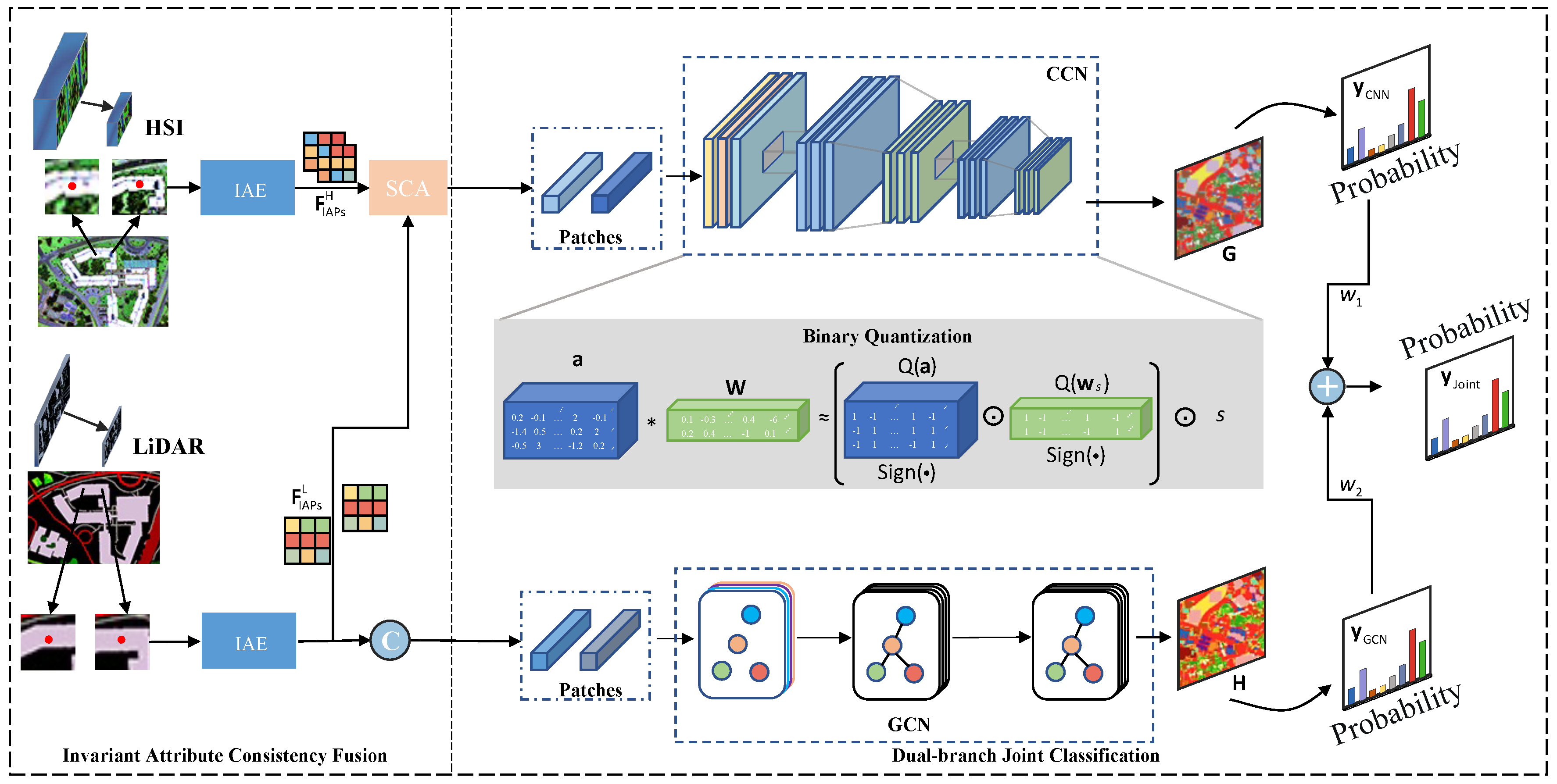
Figure 3.
Classification maps of different methods for the Houston2013 dataset.
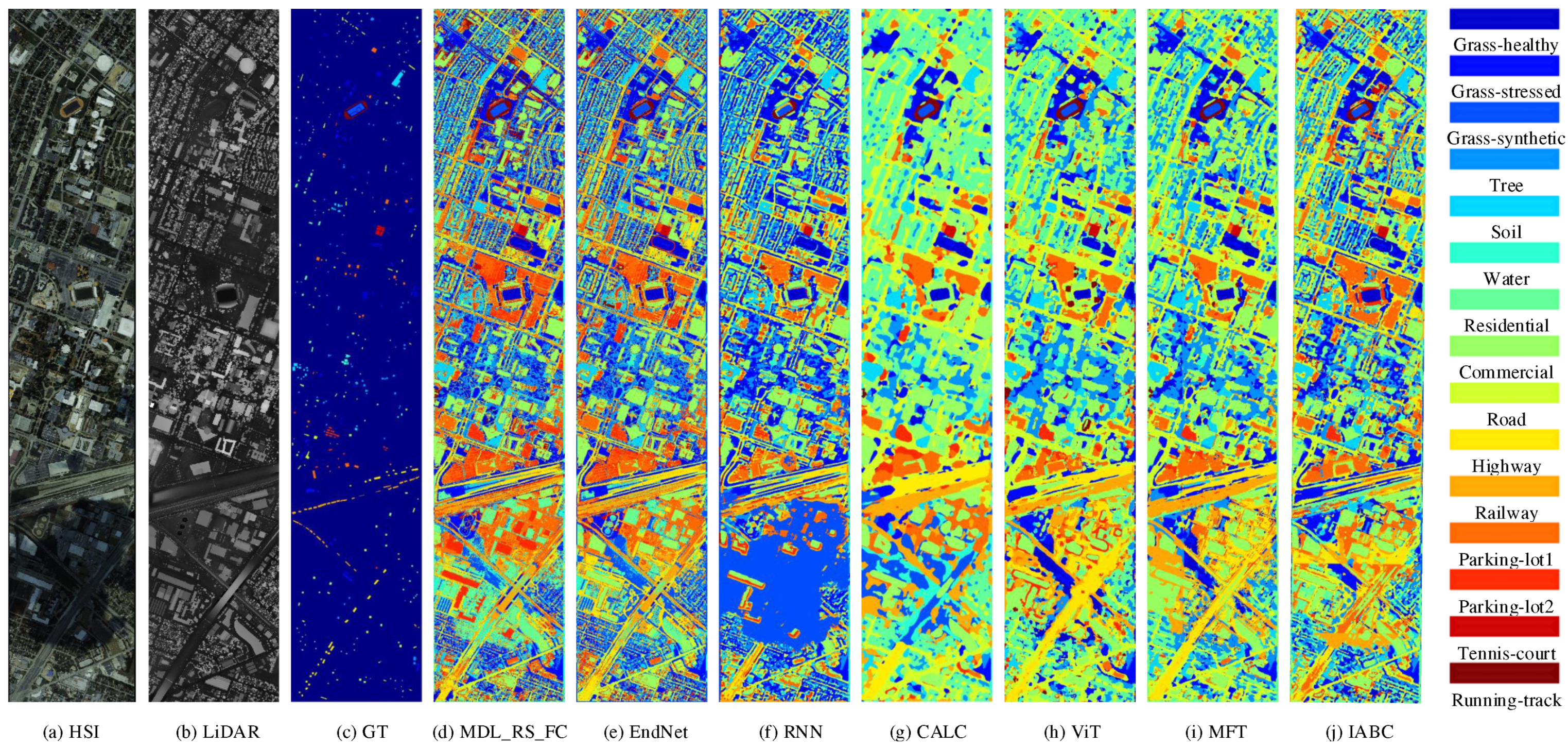

Table 1.
A list of the number of training and testing aamples for each class in Houston2013 dataset and Trento dataset.
Table 1.
A list of the number of training and testing aamples for each class in Houston2013 dataset and Trento dataset.
| Houston2013 | Trento | ||||||
|---|---|---|---|---|---|---|---|
| No. | Class Name | Training | Testing | No. | Class Name | Training | Testing |
| 1 | Healthy Grass | 198 | 1053 | 1 | Apples | 129 | 3905 |
| 2 | Stressed Grass | 190 | 1064 | 2 | Buildings | 125 | 2778 |
| 3 | Synthetic Grass | 192 | 505 | 3 | Ground | 105 | 374 |
| 4 | Tree | 188 | 1056 | 4 | Woods | 188 | 1056 |
| 5 | Soil | 186 | 1056 | 5 | Vineyard | 184 | 10317 |
| 6 | Water | 182 | 143 | 6 | Roads | 122 | 3052 |
| 7 | Residential | 196 | 1072 | Total | 853 | 21482 | |
| 8 | Commercial | 191 | 1053 | ||||
| 9 | Road | 193 | 1059 | ||||
| 10 | Highway | 191 | 1036 | ||||
| 11 | Railway | 181 | 1054 | ||||
| 12 | Parking Lot1 | 192 | 1041 | ||||
| 13 | Parking Lot2 | 184 | 285 | ||||
| 14 | Tennis Court | 181 | 247 | ||||
| 15 | Running Track | 187 | 473 | ||||
| Total | 2832 | 12197 | |||||
Table 2.
Ablation study of our proposed IACF on Houston2013 dataset.
| GCN | CNN | IAE | SCA | OA (%) | AA (%) | () | |
|---|---|---|---|---|---|---|---|
| HSI | 79.04 | 81.15 | 77.42 | ||||
| 91.15 | 91.78 | 90.38 | |||||
| 80.84 | 83.58 | 79.28 | |||||
| 88.19 | 89.31 | 87.18 | |||||
| LiDAR | 22.74 | 26.56 | 17.35 | ||||
| 35.46 | 36.33 | 30.68 | |||||
| 28.33 | 35.89 | 24.10 | |||||
| 41.81 | 39.50 | 36.90 | |||||
| HSI+LiDAR | 92.60 | 93.20 | 91.97 | ||||
| 89.46 | 90.72 | 88.55 | |||||
| 91.88 | 92.60 | 91.19 |
Table 3.
Ablation study of our proposed IACF on Trento dataset.
| GCN | CNN | IAPs | SCA | OA (%) | AA (%) | () | |
|---|---|---|---|---|---|---|---|
| HSI | 83.96 | 83.14 | 78.57 | ||||
| 95.33 | 93.95 | 93.87 | |||||
| 96.06 | 92.63 | 94.72 | |||||
| 96.93 | 93.16 | 95.88 | |||||
| LiDAR | 48.31 | 44.50 | 38.48 | ||||
| 60.26 | 63.64 | 50.67 | |||||
| 90.81 | 83.56 | 88.20 | |||||
| 68.81 | 61.33 | 61.31 | |||||
| HSI+LiDAR | 97.66 | 96.38 | 96.87 | ||||
| 97.87 | 94.04 | 97.29 | |||||
| 98.05 | 95.18 | 97.73 |
Table 4.
Validation of bi-branch joint network on Houston2013 and Trento datasets.
| Houston2013 | Trento | |||||
|---|---|---|---|---|---|---|
| OA (%) | AA (%) | () | OA (%) | AA (%) | () | |
| CNN | 91.88 | 92.60 | 91.19 | 98.05 | 95.18 | 97.73 |
| GCN | 92.60 | 93.20 | 91.97 | 97.66 | 96.38 | 96.87 |
| Joint | 92.78 | 93.29 | 92.15 | 98.14 | 97.03 | 97.50 |
Table 5.
Validation of binary quantization for CNN on Trento dataset.
| CNN | OA (%) | AA (%) | () | Params(B) | BOPs |
|---|---|---|---|---|---|
| 32w32a | 98.14 | 97.03 | 97.50 | 1045.6K | 13946.88G |
| 1w32a | 97.86 | 95.17 | 97.13 | 32.675k | 435.87G |
| 32w1a | 85.33 | 83.40 | 80.81 | 1045.6K | 435.87G |
| 1w1a | 83.44 | 77.31 | 78.01 | 32.675k | 13.62G |
Table 6.
Comparison of the classification accuracy (%) using the Houston2013 dataset.
| No. | MDL_RS_FC | EndNet | RNN | CALC | ViT | MFT | IABC |
|---|---|---|---|---|---|---|---|
| 1 | 82.15 | 82.34 | 81.80 | 80.72 | 82.59 | 82.34 | 83.10 |
| 2 | 84.40 | 83.18 | 71.40 | 81.20 | 82.33 | 88.78 | 85.15 |
| 3 | 100.00 | 100.00 | 76.04 | 93.86 | 97.43 | 98.15 | 100.00 |
| 4 | 91.48 | 91.19 | 88.51 | 96.78 | 92.93 | 94.35 | 93.18 |
| 5 | 99.15 | 99.24 | 85.76 | 100.00 | 99.84 | 99.12 | 100.00 |
| 6 | 95.10 | 95.10 | 85.78 | 95.80 | 84.15 | 99.30 | 95.80 |
| 7 | 87.50 | 83.02 | 82.77 | 93.10 | 87.84 | 88.56 | 82.46 |
| 8 | 52.99 | 76.45 | 61.44 | 92.78 | 79.93 | 86.89 | 90.41 |
| 9 | 77.34 | 71.48 | 67.42 | 82.34 | 82.94 | 87.91 | 90.84 |
| 10 | 77.32 | 64.77 | 38.45 | 67.37 | 52.93 | 64.70 | 98.94 |
| 11 | 84.06 | 88.52 | 64.39 | 98.67 | 80.99 | 98.64 | 97.82 |
| 12 | 97.21 | 94.24 | 77.07 | 97.02 | 91.07 | 94.24 | 98.46 |
| 13 | 76.49 | 76.49 | 47.13 | 82.81 | 87.84 | 90.29 | 82.81 |
| 14 | 100.00 | 100.00 | 97.98 | 99.19 | 100.00 | 99.73 | 100.00 |
| 15 | 98.52 | 98.31 | 73.50 | 100.00 | 99.65 | 99.58 | 100.00 |
| OA(%) | 84.96 | 85.03 | 72.31 | 89.79 | 85.05 | 89.80 | 92.63 |
| AA(%) | 86.91 | 86.96 | 73.30 | 90.78 | 86.83 | 91.51 | 93.26 |
| () | 83.69 | 83.81 | 70.14 | 88.95 | 83.84 | 88.93 | 91.99 |
Table 7.
Comparison of the classification accuracy (%) using the Trento dataset.
| No. | MDL_RS_FC | EndNet | RNN | CALC | ViT | MFT | IABC |
|---|---|---|---|---|---|---|---|
| 1 | 88.22 | 91.32 | 91.75 | 98.62 | 90.87 | 98.23 | 98.85 |
| 2 | 93.34 | 96.44 | 99.47 | 99.96 | 99.32 | 99.34 | 97.98 |
| 3 | 95.19 | 95.72 | 79.23 | 72.99 | 92.69 | 89.84 | 89.30 |
| 4 | 94.54 | 99.22 | 99.58 | 100.00 | 100.00 | 99.82 | 100.00 |
| 5 | 83.46 | 82.91 | 98.39 | 99.44 | 97.77 | 99.93 | 99.76 |
| 6 | 80.67 | 89.15 | 85.86 | 88.76 | 86.72 | 88.72 | 92.60 |
| OA(%) | 88.27 | 91.09 | 96.43 | 98.11 | 96.47 | 98.32 | 98.67 |
| AA(%) | 89.24 | 92.46 | 92.38 | 93.30 | 94.56 | 95.98 | 96.41 |
| () | 84.51 | 88.23 | 95.21 | 97.46 | 95.28 | 97.75 | 98.21 |
Disclaimer/Publisher’s Note: The statements, opinions and data contained in all publications are solely those of the individual author(s) and contributor(s) and not of MDPI and/or the editor(s). MDPI and/or the editor(s) disclaim responsibility for any injury to people or property resulting from any ideas, methods, instructions or products referred to in the content. |
© 2023 by the authors. Licensee MDPI, Basel, Switzerland. This article is an open access article distributed under the terms and conditions of the Creative Commons Attribution (CC BY) license (http://creativecommons.org/licenses/by/4.0/).
Copyright: This open access article is published under a Creative Commons CC BY 4.0 license, which permit the free download, distribution, and reuse, provided that the author and preprint are cited in any reuse.


