
Submitted:
19 November 2024
Posted:
20 November 2024
You are already at the latest version
Abstract
In contrast to conventional remote sensing images, hyperspectral remote sensing images are characterized by a greater number of spectral bands and exceptionally high resolution. The richness of both spectral and spatial information facilitates the precise classification of various objects within the images, establishing hyperspectral imaging as indispensable for remote sensing applications. However, the labor-intensive and time-consuming process of labeling hyperspectral images results in limited labeled samples, while challenges like spectral similarity between different objects and spectral variation within the same object further complicate the development of classification algorithms. Therefore, efficiently exploiting the spatial and spectral information in hyperspectral images is crucial for accomplishing the classification task. To address these challenges, this paper presents a Multi-Scale Feature Fusion Convolutional Neural Network (MSFF). The network introduces a dual branch spectral and spatial feature extraction module utilizing 3D depthwise separable convolution for joint spectral and spatial feature extraction, further refined by an attention based on central pixels (ACP) mechanism. Additionally, the spectral-spatial joint attention module (SSJA) is designed to interactively explore latent dependency between spectral and spatial information through the use of multilayer perceptron and global pooling operations. Finally, a feature fusion module (FF) and an adaptive multi-scale feature extraction module (AMSFE) are incorporated to enable adaptive feature fusion and comprehensive mining of feature information. Experimental results demonstrate that the proposed method performs exceptionally well on the IP, PU, and YRE datasets, delivering superior classification results compared to other methods and underscoring the potential and advantages of MSFF in hyperspectral remote sensing classification
Keywords:
hyperspectral remote sensing
; deep learning
; depthwise separable convolution
; adaptive feature extraction
; hyperspectral image classification
1. Introduction
With the advancements in imaging spectrometers and space technology, remote sensing has entered the era of hyperspectral imaging. Hyperspectral images(HSI) contain rich spatial and spectral information, covering a continuous spectrum from visible to infrared with dozens to even hundreds of narrow spectral bands, and have been widely applied in mineral exploration [1,2], environmental monitoring [3,4], agricultural assessment [5,6], medical diagnostics [7], and military target detection [8]. Hyperspectral image classification is one of the key techniques for analyzing these images. However, its classification accuracy heavily depends on the number of training samples, which are costly to label, resulting in limited availability for researchers. Additionally, due to the high spectral resolution of HSI, they are prone to the Hughes phenomenon, also known as the “curse of dimensionality,” complicating data analysis. Furthermore, the spatial resolution of spaceborne HSI, typically at the ten-meter level, can lead to spectral homogeneity for heterogeneous objects and spectral heterogeneity for homogeneous objects. Therefore, the challenge lies in how to effectively extract features and leverage the abundant spatio-spectral information to achieve accurate classification results, making it a key issue in hyperspectral image classification.
Traditional hyperspectral image classification methods often focus on spectral features or rely on statistical characteristics of the data. Common techniques include Support Vector Machines (SVM) [9], k-Nearest Neighbors (k-NN) [10], Random Forests (RF) [11], and Logistic Regression [12,13]. While these methods can classify HSI to some extent, they often extract only shallow features from the images and neglect the rich spatial information inherent in HSI. This oversight contradicts the intrinsic spatio-spectral unity of the image, leading to incomplete feature extraction [14]. Moreover, traditional machine learning models exhibit weak generalization capabilities and are often limited to specific datasets. If manually extracted features are inappropriate, classification accuracy can significantly deteriorate.
In recent years, with the rapid advancement of deep learning, this class of methods has achieved remarkable success in natural language processing and computer vision, leading to the development of numerous classical models, including Deep Belief Networks (DBN) [15], Stacked Autoencoder Networks (SAE) [16], Recurrent Neural Networks (RNN) [17], Convolutional Neural Networks (CNN) [18], among others. These deep learning methods have also been widely applied in the field of hyperspectral image classification. SAE and DBN are unsupervised learning models, which do not require a large number of labeled samples during training and are effective at reconstructing the feature information from raw data. Chen et al. [19] applied Principal Component Analysis (PCA) for dimensionality reduction of spectral information, followed by stacked autoencoder networks to extract both spectral and spatial features of HSI, ultimately achieving superior classification results using a logistic regression classifier. Zhong et al. [20] proposed a novel diversified DBN for feature extraction by integrating diversity with DBN, and ultimately classified the features using Softmax. Although these methods exploit both spatial and spectral features of HSI, their input is entirely one-dimensional, which disrupts the spatial structure of the HSI during feature extraction. A similar issue arises in models that solely utilize RNN. While RNN excel at capturing temporal dependencies in sequential data and can be applied to the spectral dimension of HSI, they are relatively inadequate at extracting spatial information from images[21].
In contrast, CNN, owing to their capability of efficiently extracting features via local connections and drastically reducing parameters through weight sharing, have, in combination with band selection algorithms [22,23,24,25], emerged as the dominant approach for hyperspectral image classification [26,27,28,29]. Hu et al. [30] proposed a five-layer 1D-CNN to extract the spectral features of classified pixels, followed by a fully connected layer for classification, pioneering the application of CNN in hyperspectral image classification tasks. Chen et al. [31] integrated Gabor filters with CNN, using Gabor filtering to extract spatial edges and intrinsic texture features from the image, followed by 2D-CNN for extracting nonlinear spatial information. Xu et al. [32] introduced the RPNet model, which treats randomly extracted image patches as convolution kernels without any need for training, and then combines shallow and deep convolutional features for classification, offering advantages of multi-scale processing and reduced computation time. Although 2D convolution methods improve accuracy over one-dimensional input models by leveraging spatial features of HSI, they are somewhat deficient in capturing spectral correlations between bands. To simultaneously extract spectral and spatial information from HSI, Chen et al. [33] introduced 3D-CNN for hyperspectral image classification, with regularization to improve model accuracy. Subsequently, Zhong et al. [34] proposed an end-to-end Spectral-Spatial Residual Network (SSRN) without preprocessing for dimensionality reduction, utilizing ResNet as the backbone and combining 3D convolution to extract spectral and spatial features through two consecutive residual modules. Roy et al. [35] introduced a hybrid CNN method called HybridSN, which first applies 3D convolution followed by 2D convolution. By combining 2D and 3D convolutions, the method compensates for incomplete feature extraction, while also effectively reducing model complexity and addressing overfitting.
Despite the superior performance of 3D-CNN-based networks, they are often accompanied by high computational demands and large parameter scales, which increase model complexity and heighten the risk of overfitting. To address these issues, researchers have begun exploring more efficient network architectures, with Howard et al. [36] gaining widespread attention for their introduction of depthwise separable convolutions. Jiang et al. [37] applied 3D separable convolutions to the ResNet architecture for hyperspectral image classification, significantly reducing the number of parameters involved in convolution operations. Similarly, Hu et al. [38] applied 3D separable convolutions to their multi-scale feature extraction module, enhancing the extraction of spatial-spectral features without increasing the number of parameters.
As discussed above, employing 3D-CNN-based networks for HSI processing effectively extracts joint spectral-spatial features. However, solely relying on convolution operations may fail to effectively focus on key parts of the data, allowing non-discriminative features to be involved in the classification process, which increases computational load and reduces classification accuracy. Therefore, enabling networks to focus more on critical details while suppressing irrelevant information from target regions has become one of the key challenges in enhancing the performance of convolutional neural networks.
To address this issue, some researchers have begun incorporating Attention Mechanisms (AM) into the architecture of deep learning networks. This mechanism enhances the model's sensitivity to discriminative features by assigning weights, while suppressing non-discriminative features [39,40,41]. Lu et al. [42] constructed a three-layer parallel residual network using convolutional kernels of three different sizes. The extracted features were then stacked and fed into a serial CBMA module, which effectively improved classification accuracy while reducing processing time. To avoid feature interference, Li et al. [43] proposed a dual-branch attention network that employs two separate branches to extract spectral and spatial features, respectively. Spatial and channel attention from CBAM is applied to the corresponding branches, and the features are finally fused for classification. Additionally, attention weight allocation based on the central pixel has been gradually developed, following the prevalent Patch-based input paradigm in hyperspectral image classification. This method often leverages the central pixel's characteristics to enhance or suppress other pixels within the patch. Zhong et al. [44] established pixel relationships by calculating the cosine similarity between the central pixel and its surrounding pixels within the patch. Similarly, Li et al. [45] designed a two-branch self-similarity module based on cosine and Euclidean similarity, deeply exploring the spatial relationships guided by the central vector within the patch, thereby enhancing the efficiency of subsequent feature extraction.
Inspired by these above work, a Multi-Scale Feature Fusion Convolutional Neural Network is proposed for hyperspectral image classification in this paper. In MSFF, two convolutional layers with different kernel sizes are utilized to independently extract spectral and spatial features, and an ACP module is designed to capture the relationships between the central pixel and its neighboring pixels. Subsequently, a global attention mechanism and a feature fusion module are applied to minimize noise interference and focus on key feature information. Finally, an Adaptive Multi-Scale Feature Extraction module is employed to optimize the extracted feature information, enable adaptive selection and fusion of multi-level features, thereby capture more representative features for classification in the fully connected layer. The main contributions of this article are as follows.
- To enhance sensitivity to salient information in both spatial and spectral dimensions, the SSJA module is proposed. This module jointly models the independently extracted global spatial and channel features via a MLP to reveal their correlations. This approach effectively captures the latent dependencies between spatial and spectral features, allowing the attention weights to account for global information.
- To address the problem of insufficient feature extraction, multiple multi-scale strategies are introduced in the model and the AMSFE module is proposed to gather supplementary information from different levels, enable feature reuse and extraction of more representative features. Additionally, low-parameter or even parameter-free attention mechanisms are embedded in the front, middle, and back stages of the model, ensuring accurate and efficient object identification.
- To reduce model complexity and mitigate overfitting, 3D depthwise separable convolution layers are used to replace standard 3D convolution layers . This replacement optimizes computational efficiency and reduces overfitting risk while maintaining high classification accuracy.
The paper is structured as follows: Section 2 details the MSFF design and core mechanisms. Section 3 presents the datasets and analyzes experimental results to demonstrate model effectiveness. Section 4 discusses the method’s advantages, and Section 5 concludes with key insights and future directions.
2. Methods
This section introduces the proposed network structure, covering the spatial and spectral feature extraction modules, the spectral-spatial joint attention module, feature fusion, and adaptive multi-scale extraction modules. The overall architecture is shown in Figure 1.
Before model training, hyperspectral data undergoes preprocessing with PCA to reduce channel redundancy. To leverage spatial information, neighboring pixels are extracted from the reduced data, forming 3D inputs for the model.
The data first passes through a 3D depthwise separable convolution with a kernel size of (7, 3, 3) and a spectral stride of 2, extracting spatial-spectral features and reducing dimensionality. The output is then fed into spectral and spatial feature extraction modules for deeper feature extraction. The combined results are sent to the joint attention and feature fusion modules to focus on key classification features. Finally, the weighted features pass through the adaptive multi-scale feature extraction module to complete the classification. The model architecture is shown in Figure 2, with the input 3D cube set to 30×11×11 for clarity.
2.1. Spectral And Spatial Feature Extraction
The SSFE module is built upon several core technologies, which are introduced in this section.
2.2.1. Three-Dimensional Depthwise Separable Convolution
Given the inherently three-dimensional nature of hyperspectral images, traditional 2D convolution methods exhibit limitations in extracting shallow features. While 2D convolution excels at processing spatial information, it fails to fully leverage spectral data, potentially overlooking crucial inter-band relationships and weakening the extraction of comprehensive spectral features. In contrast, 3D convolution performs simultaneously across both spatial and spectral dimensions, effectively capturing joint spectral-spatial features. However, despite the superior feature extraction capability of 3D convolution, it often requires substantial parameters and computational power, posing significant challenges for hyperspectral image classification with limited sample sizes. To address these challenges, we introduce the concept of 3D depthwise separable convolution, which combines 3D depthwise and pointwise convolutions to reduce computational complexity.
In traditional 3D convolution, each kernel must process every channel of the input features to generate a feature map, as depicted in Figure 3. Assuming the kernel size is K in all directions, the total number of parameters for 3D convolution can be expressed as Num3d=K×K×K×M×N, where M represents the input channels, and N represents the output channels. The computational cost of 3D convolution is given by Cost3d=K×K×K×M×N×C×H×W, where (C, H, W) represent the dimensions of the feature map, and padding is applied to preserve the feature map size.
The process of 3D depthwise separable convolution is composed of two key stages: 3D depthwise convolution and 3D pointwise convolution, as illustrated in Figure 4. The first stage involves 3D depthwise convolution, where the convolution kernel operates exclusively within a single channel, meaning each channel of the feature map is convolved independently with its own kernel, producing an output feature map that retains the same number of channels as the input. The parameter count for this step can be expressed as Num3dp=K×K×K×M, and the computational cost is given by Cost3dp=K×K×K×M×C×H×W. As the 3D depthwise convolution applies independent operations on each input channel, it fails to capture inter-channel relationships at corresponding spatial locations and cannot increase the number of output channels. Therefore, 3D pointwise convolution is required to further refine the features. The 3D pointwise convolution operates similarly to standard convolution, but with a kernel size of 1, where the input channel count is M. In this stage, the convolution performs a weighted combination of the features obtained in the previous step along the depth dimension, resulting in a new feature map. The number of parameters in this stage is Num3pw=M×N, and the computational cost is Cost3pw=M×N×C×H×W. Summing the parameters and computational costs from both stages yields the total parameter count and computational cost for the entire 3D depthwise separable convolution operation, expressed as Num3dw=K×K×K×M+M×N and Cost3dw=K×K×K×M×C×H×W+M×N×C×H×W, respectively. To assess the effectiveness of 3D depthwise separable convolution in alleviating the computational and parameter burdens, the following calculations can be made.
According to the above formula, it can be seen that the three-dimensional depth separable convolution has significantly reduced parameters and computational complexity compared to ordinary three-dimensional convolution, especially when the output channel and convolution kernel size increase, the reduction ratio is more obvious.
2.1.2. ACP
In conventional hyperspectral image classification tasks, the pixels surrounding the target pixel are extracted, forming a cube that serves as input to the model. This approach aims to leverage spatial context to enhance classification accuracy. However, while neighboring pixels contribute unequally to the classification compared to the center pixel, convolution operations are unable to capture the underlying relationships between the center pixel and its surrounding pixels. To address this limitation, we developed an attention based center pixel (ACP) module, which calculates the Euclidean similarity between the center pixel and its neighboring pixels to capture their relationships. The architecture is illustrated in Figure 5.
After computing the Euclidean similarity between each vector and the center vector, a weight map is generated, maintaining the same spatial dimensions as the input feature map. Subsequently, the input feature map is multiplied by the calculated weights and summed, thereby emphasizing the most significant features. The Euclidean similarity is calculated using the formula presented in Equation (3).
denotes the Euclidean similarity between vectors. Given a block size of r×r, represents the central vector, where o=r/2, with i = 1,...,r and j= 1,...,r.
2.1.3. Spectral and Spatial Feature Extraction
The spatial and spectral feature extraction module proposed in this study is depicted in Figure 6. Except for the differences in convolution kernel sizes, the two branches share an identical structure. Convolution kernels of (7,1,1) and (1,3,3) are employed to extract spectral and spatial features from the data, respectively. By decoupling and independently processing information across different dimensions, the network can more effectively capture distinctive features of various classes in hyperspectral images. Following several convolutional and residual connection operations, the data is reshaped from three-dimensional to two-dimensional form, with the ACP module introduced to capture the relationships between the center pixel and its neighboring pixels. Finally, the outputs from both branches are summed.
2.1. SSJA
In our examination of existing deep networks, we observed that the majority of networks tend to adopt independent methods for obtaining spatial and spectral attention weights. While this approach ensures that the model concentrates more effectively on each individual dimension during feature extraction, it may inadvertently result in the loss of interaction information between these dimensions. To address this issue, we introduce the SSJA module, inspired by CBAM, to derive attention weights that account for global information while capturing the potential dependencies between spatial and spectral dimensions.
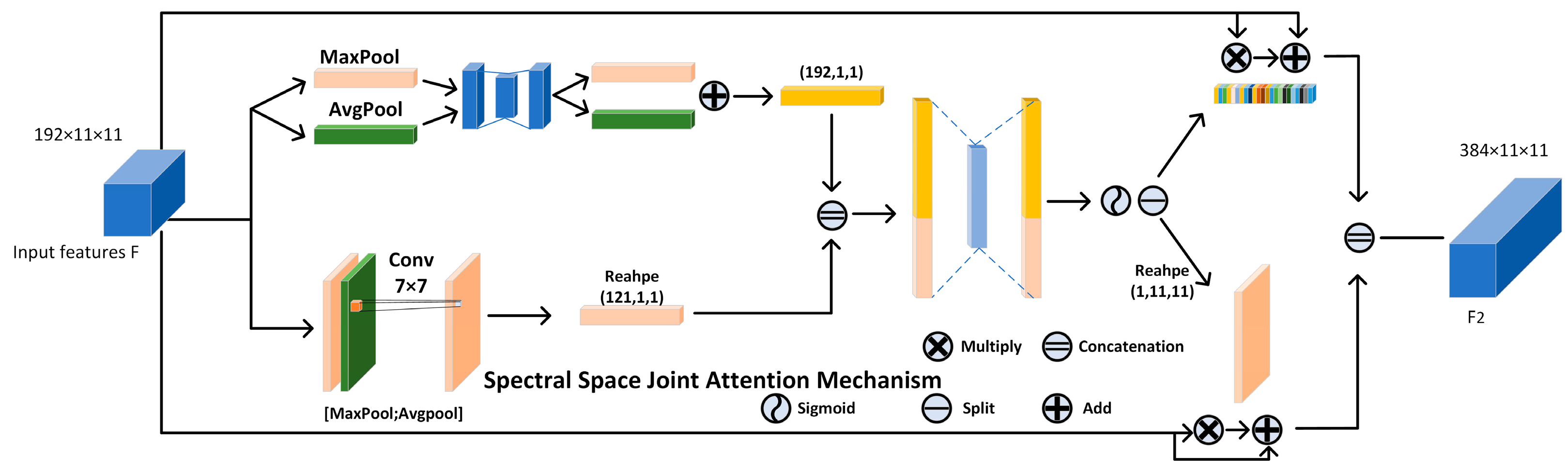
Figure 7.
The proposed SSJA structure.
Initially, the data is processed through two separate branches. In the upper branch, the input features are subjected to global max pooling and global average pooling along the spatial dimension, enabling the capture of subtle semantic variations within the data. Subsequently, the pooled results are fed through a shared-parameter multilayer perceptron to extract spectral attention features. The two resultant vectors are then summed, as expressed in Equation (4).
denotes the input feature, while and denote global average pooling and global max pooling along the spatial dimension executed on , respectively, and refers to the shared-parameter multilayer perceptron.
In the lower branch, the input undergoes global max pooling and global average pooling along the channel dimension, after which the results are concatenated. A 7×7 convolution kernel then integrates the semantic information from the concatenated data. The fused output is reshaped into a one-dimensional vector to facilitate subsequent operations, as outlined in Equation (5).
denotes the 7×7 convolution operation, while and refer to global average pooling and global max pooling along the channel dimension, respectively. signifies the reshape operation, which flattens the data into a one-dimensional vector, and represents the concatenation.
Subsequently, the two one-dimensional vectors, and , are concatenated along their lengths to form a feature vector encapsulating both spectral and spatial semantic information. This vector is then fed into a multilayer perceptron to model the relationships between spectral and spatial dimensions. The output of this modeling is passed through a Sigmoid activation function to enhance the non-linear representational capacity, yielding an attention vector that integrates both spectral and spatial features. The attention vector is then split and reshaped back to its original form. These vectors are multiplied and summed with the input features, and then concatenated along the channel dimension, resulting in feature maps with distinct attention weights. This process is captured by Equations (6), (7), and (8).
In these equation,anddenote the channel attention weights and spatial attention weights, respectively, after splitting and reshaping.indicates the reshape operation that restores the data to its original form, andrepresents the concatenated output of the module.
2.3. FF
In the final operation of the previous step, instead of directly adding the two features with different dimensional attention, we opted to concatenate them, since simple addition does not efficiently integrate their information. As a result, an adaptive fusion method was devised, as illustrated in Figure 8.
First, the input feature map F2 undergoes global average pooling and global max pooling along the spatial dimension. The two resulting one-dimensional vectors are concatenated spatially and then processed by a 2×1 convolution to integrate the distinct feature distributions. Afterward, the weights are computed using the Softmax function and applied to the input features via multiplication and summation. Since the concatenation in the previous module doubled the channel size, a 1×1 convolution is employed at the end to reduce the dimensionality. This process is mathematically represented as follows.
whereandrefer to convolutions with kernel sizes of 2×1 and 1×1, respectively.anddenote the global average pooling and max pooling operations on, andrepresents the final output of this module.
2.4. AMSFE
This section introduces the core technologies that make up the AMSFE module.
2.4.1. NAM
To improve the model's sensitivity to key features while preserving its lightweight architecture, we introduce an attention mechanism that computes attention weights exclusively using the scaling factor from batch normalization, without introducing additional parameters. The structure of this approach is shown in Figure 9.
Initially, the scaling factoris learned through the batch normalization (BN) process, as described in Equation (11), where and denote the mean and standard deviation of batch , and stands for the bias term. As the scaling factor corresponds to the variance in BN, it directly reflects the importance of each channel. A larger variance indicates greater fluctuations in the channel, signifying that it contains more information and is therefore more critical. In contrast, a smaller variance signifies lower importance.
The resulting scaling factor is then applied using Equation (12), producing weight factors that represent the proportional scale of each channel relative to the others. Next, we multiply the features processed in Equation (11) by these weight factors on a per-channel basis. A final Sigmoid activation is applied to enhance non-linearity, yielding the channel-specific weights , as represented by Equation (13).
2.4.2. AMSFE
In general hyperspectral image classification tasks, diverse land cover types are typically present, and the contextual information needed for different object categories can vary greatly. As a result, the model must capture multi-scale feature information to accurately classify the various categories. Generally, shallow features offer richer detail and higher resolution, though they are often accompanied by noise. In contrast, deeper features convey robust semantic information but tend to lack finer details. Therefore, we developed an adaptive multi-scale feature extraction module that equips the model with the ability to selectively and adaptively fuse features across different layers, thereby improving its generalization capability and enhancing classification accuracy. The structure is illustrated in Figure 10.
Initially, the input features are processed through a convolution operation with a kernel size of 5 and 128 channels, aimed at reducing both the spatial resolution and channel dimensionality. The downsampled features are then passed through multiple densely connected 2D convolutions, extracting features across varying scales from shallow to deep layers. The dense connections are employed to prevent gradient vanishing over successive convolutions. The output after every two convolutions is treated as a feature representation at one scale. For clarity, we illustrate the process using four convolutions, corresponding to two different scales. Once the features from different scales are obtained, we apply an additional convolution with a kernel size of 1 and 64 channels to further refine these features and adjust the number of channels at each scale. We then apply a parameter-free attention mechanism NAM to enhance the precision of the information encapsulated within both features. In this context, two convolutions—one with a kernel size of 1—alongside one NAM operation, are grouped into what we define as a Feature Extraction Group (FEG). The number of FEG can be treated as a hyperparameter in the experimental setup. To obtain the fusion weights for the multi-scale features, we first sum them and then apply global average pooling to the result. The pooled vector is subsequently passed through a funnel-shaped fully connected layer, where the second layer generates a vector with the same number as the summed features. Next, a Softmax function is applied at each corresponding position of the vector to derive the weights for each feature channel. Finally, the input features are multiplied by their corresponding weights, and the updated features are summed to yield a fused multi-scale representation. This process is formally expressed by the following equation.
and denote features from different scales that have been processed by the FEG. represents fully connected layer, while and represent the vectors obtained after passing through the fully connected layer. and correspond to the fusion weights of features and , respectively, and denotes the final fused feature.
Finally, the fused feature is flattened and passed through a series of two fully connected layers to generate the classification result.
3. Experimental Results and Discussion
We conducted experiments on two public datasets alongside one self-annotated dataset. All experiments were carried out under consistent hardware configurations, comprising an AMD Ryzen 5 5600 6-core processor, 16GB of RAM, and an NVIDIA GeForce RTX 3060 Ti GPU. The experimental setup included a Windows 11 operating system, the PyTorch 1.12.0 deep learning framework, and CUDA 11.3 for GPU acceleration.
3.1. Datasets
The datasets employed in the experiments include Indian Pines, Pavia University, and Yellow River Estuary coastal wetland. The first two are publicly available, while the latter is self-annotated.
Indian Pines (IP): The Indian Pines dataset is one of the earliest benchmarks for hyperspectral image classification. Captured by the Airborne Visible/Infrared Imaging Spectrometer (AVIRIS) in 1992, it covers a pine forest in Indiana, USA, with a 145×145 region annotated for classification. The AVIRIS sensor captures wavelengths in the 0.4–2.5 μm range with 220 spectral bands. Due to water absorption, bands 104-108, 150-163, and 220 are excluded, leaving 200 bands for most research. With a spatial resolution of around 20 meters, the dataset is prone to mixed pixels, complicating classification. Figure 11a,b show the false-color image and ground truth labels. The dataset contains 21,025 pixels, with 10,249 corresponding to land-cover classes, and the remaining 10,776 as background, excluded from classification. The region consists mostly of agricultural land, with 16 distinct land-cover types. However, the sample distribution is highly imbalanced, and spectral similarities between classes further increase classification difficulty. The pixel distribution for each class is presented in Table 1.
Pavia University (PU): The Pavia University dataset is a hyperspectral image subset captured in 2003 over Pavia, Italy, by the Reflective Optics Spectrographic Imaging System (ROSIS-03). The system captures spectral data across 115 bands in the 0.43–0.86 μm range, with a spatial resolution of 1.3 meters. Due to noise, 12 bands were discarded, leaving 103 bands for analysis. Figure 11c,d show the false-color composite and ground truth labels. The dataset measures 610×340 pixels, comprising a total of 2,207,400 pixels. However, a significant proportion are background pixels, with only 42,776 pixels corresponding to land-cover types, as detailed in Table 2.
Yellow River Estuary coastal wetland(YRE): The YRE dataset was collected in 2019 over the Yellow River Delta Nature Reserve core area, Dongying, Shandong Province, China, by GF5_AHSI. The image consists of 330 spectral bands spanning wavelengths from 390–1029 nm (VNIR) and 1005–2513 nm (SWIR). Due to noise interference, 50 corrupted bands were excluded, leaving 280 spectral bands for classification purposes. The spatial resolution of the dataset is 30 meters. To enhance spatial resolution and mitigate the impact of mixed pixels, the panchromatic band of Landsat 8 imagery was fused with GF5 hyperspectral data using the Gram-Schmidt transformation method, improving the resolution to 15 meters. Figure 11e,f display the false-color image and ground truth following the fusion process. The dataset measures 710 × 673 pixels, containing 477,830 pixels in total. Of these, only 79,732 pixels from 9 distinct land-cover types were annotated for classification, as detailed in Table 3.
3.2. Evaluation Metrics
To assess the classification performance of the proposed model, we employ overall accuracy (OA), average accuracy (AA), and the Kappa coefficient as key evaluation metrics. These metrics serve as pivotal indicators in determining the efficacy of hyperspectral image classification algorithms; higher values denote stronger model classification capabilities. Assuming the confusion matrix is represented as a c×c matrix, where c indicates the number of classes andrepresents the number of samples from class j that are classified as class i, the metrics can be formulated as follows.
OA:The ratio of correctly classified targets to the total number of targets in the test set. Its formula is given as follows.
AA: The average percentage of correctly classified pixels for each class, obtained by calculating the proportion of correctly classified pixels in each class relative to the total number of pixels, and then averaging these proportions across all classes. Its formula is given as follows.
Kappa coefficient: A statistical measure of agreement between classification results and ground truth, employing a discrete multivariate approach to mitigate OA’s bias toward class and sample size. Its formula is given as follows.
3.3. Experimental Parameters
To achieve optimal model performance, we conducted experiments on key hyperparameters that have a significant impact on classification accuracy. These include batch size, patch size, number of channels, and the number of feature extraction groups (FEG) proposed in the AMSFE module. In these experiments, we employed the cross-entropy loss function and Adam optimizer for network optimization, with a learning rate of 0.0001 and 150 training epochs. Given the significant variation in sample size and class distribution across the datasets, we randomly selected 10% of the samples from the IP dataset, which has fewer samples, for training. For the PU and YRE datasets, with larger sample sizes and more balanced class distributions, we selected 5% and 1% of the samples, respectively, for training, while the remaining data were used for testing.
3.3.1. Batchsize
Batch size is a critical hyperparameter in model training, representing the number of training samples used in each forward and backward propagation. The selection of batch size can significantly influence the efficiency, stability, and convergence rate of the training process. Larger batch sizes improve training speed and hardware utilization, but excessive sizes can cause memory limitations and potentially overlook features of rare samples. Therefore, we conducted experiments with batch sizes of 32, 64, 128, 256, and 512 across the three datasets, and the results are presented in Figure 12.
For the IP dataset, we observed that when the batch size was set to 32, all three metrics achieved their peak values. As the batch size increased, these metrics exhibited a general downward trend, with average accuracy (AA) experiencing the most pronounced decline. This phenomenon is primarily due to the severely imbalanced sample distribution in the IP dataset. As batch size increases, the model's sensitivity to minority class samples diminishes, causing it to prioritize overall accuracy at the expense of minority class precision, thereby leading to a substantial drop in AA. For the PU and YRE datasets, accuracy followed a trend of initial increase followed by a decrease, with relatively stable fluctuations. The variation in accuracy for both datasets remained within 0.4%. The optimal batch sizes for PU and YRE were 64 and 128, respectively.
3.3.2. Patchsize
Patch size is another critical parameter influencing model performance. It refers to the size of the local region used to extract data from the original hyperspectral image. If the window is too small, it may lead to insufficient spatial feature representation, resulting in the loss of valuable contextual information. Conversely, if the window is too large, it may incorporate pixels from surrounding classes, increasing noise in the data and thus lowering classification accuracy. Therefore, determining an optimal patch size that aligns with the characteristics of each dataset is crucial. To this end, we experimented with six different window sizes—7×7, 9×9, 11×11, 13×13, 15×15, and 17×17 across the three datasets, with the results presented in Figure 13.
For the IP dataset, we observed that patch size significantly influences the model’s classification accuracy, particularly as the window size increases from 7 to 11, resulting in marked improvements across all metrics. The model achieves its optimal performance when the patch size reaches 15. Although the class distribution in the IP dataset is imbalanced, the spatial distribution of each class is relatively concentrated. This minimizes the noise introduced by larger patch sizes, enabling better performance with larger windows. For the PU and YRE datasets, the line graphs reveal trends similar to the IP dataset, showing an initial rise followed by a decline. Smaller window sizes do not notably affect the YRE dataset; however, accuracy declines markedly with larger window sizes. This may be because the YRE dataset contains a higher proportion of edge pixels, so larger patch sizes introduce more noise, resulting in decreased accuracy. The optimal patch sizes for PU and YRE were 13 and 11, respectively.
3.3.3. Channel Numbers
The spectral dimension of hyperspectral remote sensing images offers highly informative data for feature extraction, but the increase in spectral bands inevitably introduces more redundancy and adds complexity to the data processing pipeline. Consequently, the number of channels retained after PCA transformation becomes a critical hyperparameter that directly influences the classification accuracy. To investigate this, We evaluated the performance on three datasets with retained channel numbers of 20, 25, 30, 35, and 40, as shown in Figure 14.
As shown in the figure, the optimal number of channels is 30 for both the IP and YRE datasets, whereas for the PU dataset, it is 20. The PU and YRE datasets show stable performance with fewer retained bands, while the IP dataset underperforms in similar conditions. This discrepancy likely stems from the IP dataset's larger variety of classes, requiring more spectral bands to capture each class’s distinct features.
3.3.3. FEG Numbers
In the final module of the proposed model, we introduce the FEG structure to capture feature information at varying depth scales within the convolutional layers. When the number of FEG is too high, it may increase the model parameters, potentially resulting in overfitting. Conversely, when the number is too low, feature extraction may become insufficient, adversely affecting the model's performance. Therefore, we conducted experiments using FEG counts of 0, 1, 2, and 3 across three datasets, as presented in Figure 15.
According to the figure, we observed that setting the number of FEG to 2 yielded optimal performance across all three datasets. The accuracy gains achieved through FEG validate its effectiveness in capturing multi-scale features, demonstrating its positive impact on enhancing the model's generalization ability.
These four sets of experiments allowed us to identify the optimal hyperparameters for each dataset, as detailed in Table 4.
3.4. Comparative Experiment
To validate the classification performance of the MSFF model, we conducted comparative experiments against eight other network models, including 2D-CNN, SSRN, DBMA, HybridSN, MDRDNET, SSTFF, DMAN, and a modified version of the MSFF model where the SSJA module is replaced with the CBAM module (MSFF-CBAM). To ensure fairness, we used the optimal parameters recommended by the original authors for each of the comparison methods. The datasets were divided into training and test sets, with 10%, 5%, and 1% of the samples used for training on the IP, PU, and YRE datasets, respectively, while the remaining samples were designated for testing. Finally, OA, AA, and Kappa were employed as evaluation metrics. The classification accuracies for all methods are presented in Table 5, Table 6 and Table 7, with the corresponding classification maps shown in Figure 16, Figure 17 and Figure 18.
3.4.1. Experimental Results of IP
As indicated in Table 5, our model attained the highest values across all three metrics for the IP dataset, with OA, AA, and Kappa achieving 99.14%, 99.05%, and 99.02%, respectively. Table 1 reveals that the IP dataset demonstrates significant disparities in sample counts across different classes. The Alfalfa class contains only 4 training samples, while Grass-pasture-mowed and Oats have just 2, in contrast to Soybean-mintill, which contains 245, the largest sample size. This suggests that classifying the IP dataset poses a significant challenge to the model's ability to accurately extract features from small sample sizes. Models like HybridSN and MDRD-Net, which employ numerous 3D and 2D convolution operations, show good performance in terms of OA, achieving 98.79% and 98.66%, respectively. However, the significant discrepancy between their AA and OA values indicates that these models may overfit certain classes, leading to insufficient generalization ability. DBMA, a full-spectrum model that forgoes dimensionality reduction preprocessing, performed poorly, ranking second-worst after 2D-CNN. Despite employing dual network branches to extract spectral and spatial features, DBMA considers features only at a single scale. The model's reliance on large convolutional kernels and extensive pooling operations resulted in excessive loss of critical information, leading to suboptimal performance on the IP dataset. The 2D-CNN model was the poorest-performing method among all comparisons, and the reason is evident—relying solely on 2D convolutions is inadequate for extracting features from 3D data. While MSFF model did not achieve perfect classification accuracy for small-sample classes such as Alfalfa and Oats, the number of misclassifications remained within a narrow range of 1 to 3 samples. Additionally, for the Corn-notill class, containing 1428 samples, the model attained 100% classification accuracy. Moreover, Our model outperformed all comparison methods in seven categories, highlighting its significant performance advantages.
3.4.2. Experimental Results of PU
In the experiments on the PU dataset, MSFF outperformed all other comparison models, achieving OA, AA, and Kappa values of 99.73%, 99.56%, and 99.64%, respectively. On the PU dataset, full-spectrum models demonstrated a clear advantage over dimensionality-reduced approaches. Both DBMA and SSRN yielded strong results, with DBMA advancing from second-to-last on the IP dataset to second-best on the PU dataset, with its OA only 0.06% lower than that of our model. This improvement can be attributed to the PU dataset’s composition, with only nine land-cover classes and 103 spectral bands, significantly reducing spectral redundancy compared to the IP dataset's 200 bands, enabling full-spectrum models to better capitalize on their strengths. Among the dimensionality-reduced models, SSTFF ranked just behind MSFF, achieving the third-highest performance overall. This is largely attributed to its effective architecture, which combines CNN for local feature extraction and Transformers for long-range dependency modeling, boosting overall performance. HybridSN, which ranked second on the IP dataset, performed poorly on the PU dataset, finishing second-to-last. Our parameter search revealed that larger patchsize were unsuitable for the PU dataset. HybridSN use of a 25-size window, without incorporating multi-scale strategies to alleviate the issues of larger windows, likely contributed to its underperformance on the PU dataset. In conclusion, while MSFF performance was not significantly higher than the comparison methods, it still delivered the best overall results.
3.4.3. Experimental Results of YRE
In the YRE dataset, where relatively pure pixels were labeled and the category distribution was balanced, all methods achieved the highest accuracy across the three datasets, despite only 1% of the samples being used for training. Our model continued to outperform others, with OA, AA, and Kappa values of 99.96%, 99.95%, and 99.95%, respectively. DMAN performed nearly as well as MSFF, with its OA, AA, and Kappa scores trailing by only 0.02%, 0.03%, and 0.02%, respectively. This performance can be attributed to its model architecture, which effectively handles small sample sizes by leveraging multi-scale strategies and hybrid convolution modules to counter insufficient feature extraction and overfitting. Full-spectrum models like DBMA and SSRN exhibited a slight decline in performance on the 280-band YRE dataset. Although their accuracy remained comparable to other models, they were ranked second-to-last and third-to-last. MDRD-Net achieved its highest ranking across all three experiments, while HybridSN and SSTFF delivered consistently stable performance. Overall, MSFF generated classification maps most closely aligned with the ground truth.
Comparing results across the three datasets, MSFF consistently surpassed MSFF-CBAM in classification accuracy, demonstrating that the SSJA module offers superior feature localization capabilities within our model architecture, positively impacting classification performance. This also validates the significance of integrating global information interaction in model design.
3.5. Ablation Study
To verify the effectiveness of each module in MSFF, ablation experiments were performed across three datasets. As the FEG in AMSFE had already been quantitatively analyzed during parameter selection, this section concentrates on evaluating the ACP, SSJA, and FF modules. These modules were combined in various configurations, as illustrated in Table 8, with the corresponding results shown in Figure 19. OA was the sole evaluation metric used in the experiments, while all other parameters remained consistent with the comparison experiments.
Figure 19 shows that all datasets exhibit a similar trend: individual modules underperform compared to any two-module combinations, and the S6 configuration achieves the best results across all datasets. However, due to the varying characteristics of each dataset, the contribution of each module to performance differs. SSJA made a substantial contribution to the IP dataset, boosting the accuracy of the S0 model by around 0.7%. Conversely, ACP combined with other structures produced less impressive results, often resulting in minimal or no improvement. This trend was also seen in the YRE dataset, likely because ACP is a parameter-free attention mechanism without a training process, making its impact weaker than parameterized structures. Furthermore, ACP performance depends on the dataset's spatial resolution—higher pixel clarity leads to better results. In contrast, ACP performed better in the PU dataset with a 1.5m spatial resolution. FF contributed more to the PU dataset than SSJA. Comparing this to the accuracy of the S0 model, we found that simpler attention mechanisms work better for this dataset. Even the top-performing S6 structure only surpassed S0 by roughly 0.2%, likely due to the limited number of categories, allowing simple attention mechanisms to capture most of the relevant features. The combination of SSJA and FF achieved the best results across all three datasets, primarily due to their well-structured designs and the substantial number of trainable parameters. After SSJA extracts spatial and spectral features, FF fuses this information and reduces dimensionality, aligning with standard feature extraction principles. Finally, comparing the accuracy from Figure 18 with the results of the comparison experiments, the complete MSFF model continued to deliver the best performance.
4. Discussion
In the aforementioned study, we observed that optimal parameter selection and network architecture design are crucial to enhancing model performance. For instance, as demonstrated in our patch size experiments, merely increasing the window size from 7 to 11 on the IP dataset led to an impressive 4% increase in accuracy, a gain that exceeded improvements achieved by fine-tuning other models. Although different parameters can be tested across datasets to find optimal values, designing a model tailored to a single dataset is resource-intensive and inefficient. Thus, developing a generalized network architecture capable of adapting to multiple environments is essential for successful hyperspectral image classification. From the comparison experiments, we observed that despite MDRD-Net and HybridSN sharing similar architectural designs, with MDRD-Net containing only half the parameters of HybridSN, the former consistently outperformed the latter on all three datasets. This is likely due to MDRD-Net’s strategic use of multi-scale feature extraction, attention mechanisms, and residual connections to enhance model depth, which together improve its ability to capture and understand complex data features. However, MDRD-Net lacks a dedicated information fusion module, instead relying on simple summation to combine information from different branches. In contrast, DMAN and SSTFF address this more effectively: DMAN integrates information from different dimensions using pooling and convolution operations of varying sizes, smoothing feature loss through bilinear interpolation, while SSTFF employs the multi-head self-attention mechanism from Transformer to capture and fuse feature vectors from its SSFE module. Despite their differing approaches, both methods aim to fuse features, allowing the model to gain a more comprehensive understanding of the data.
Although MSFF generally delivers strong results, its performance on imbalanced datasets, particularly in small-sample categories, remains imperfect. Moreover, the model contains a significant number of convolution operations; while depthwise separable convolutions help reduce parameter count, the total still exceeds 2 million. Therefore, in future work, we will focus on addressing the small-sample challenge and aim to design a more lightweight model.
4. Conclusion
A multi-scale feature fusion convolutional neural network model tailored for hyperspectral image classification tasks was introduced in this paper. The proposed approach utilizes a dimensionality-reduced 3D data block, representing the target pixel and its surrounding neighborhood, as input data. Initially, the input undergoes processing via two separate 3D convolutional layers, each employing distinct kernel sizes, to extract shallow-level features. Subsequently, the outputs from both branches are aggregated and fed into the attention module, enhancing the model’s focus on critical regions within the data. Following the attention mechanism, the feature map is directed into a feature fusion module, where adaptive channel fusion occurs via convolution operations, yielding a more comprehensive feature representation. Finally, the classification task is performed within a multi-scale feature extraction module. Comparative experiments were conducted on two public datasets and one self-annotated dataset, to achieve fine classification of forest, urban, and coastal wetland land cover types, with overall accuracies of 99.15%, 99.73%, and 99.96%, respectively, outperforming all other methods.
Future research will prioritize reducing the substantial parameter count and complexity of convolutional neural network architectures. Moreover, exploring effective strategies for leveraging unlabeled data to mitigate sample insufficiency will also be a critical focus moving forward.
Author Contributions
Conceptualization, G.G. and X.W.; methodology, G.G. and X.W.; software, G.G. and Z.P.; validation, Z.L., J.Z. and Z.P.; formal analysis, X.W. And X.S.; investigation, G.G.; resources, J.Z.; data curation, G.G.; writing—original draft preparation, G.G.; writing—review and editing, X.W.; visualization, G.G.; supervision, X.W.; project administration, X.S.; funding acquisition, J.Z. All authors have read and agreed to the published version of the manuscript.
Funding
This work was jointly supported by the Central Guiding Local Science and Technology Development Fund of Shandong—Yellow River Basin Collaborative Science and Technology Innovation Special Project (No. YDZX2023019), the Shandong Key Research and Development Project (No. 2018GNC110025, No. ZR2020QF067), the National Natural Science Foundation of China (No. 42301380, No. 42106179), the Qingdao Natural Science Foundation Grant (No. 23-2-1-64-zyydjch), and the Science and Technology Support Plan for Youth Innovation of Colleges and Universities of Shandong Province of China (No. 2023KJ232).
Data Availability Statement
The Indian Pines dataset and the Pavia University dataset are available at https://www.ehu.eus/ccwintco/index.php/Hyperspectral_Romte_Sensing_Scenes
Conflicts of Interest
The authors declare no conflicts of interest.
References
- Tan, K.; Wu, F.; Du, Q.; Du, P.; Chen, Y. A Parallel Gaussian–Bernoulli Restricted Boltzmann Machine for Mining Area Classification With Hyperspectral Imagery. IEEE J. Sel. Top. Appl. Earth Obs. Remote Sens. 2019, 12, 627–636. [Google Scholar] [CrossRef]
- Okada, N.; Maekawa, Y.; Owada, N.; Haga, K.; Shibayama, A.; Kawamura, Y. Automated identification of mineral types and grain size using hyperspectral imaging and deep learning for mineral processing. Minerals 2020, 10, 809. [Google Scholar] [CrossRef]
- Ghamisi, P.; Plaza, J.; Chen, Y.; Li, J.; Plaza, A.J. Advanced Spectral Classifiers for Hyperspectral Images: A Review. IEEE Geosci. Remote Sens. Mag. 2017, 5, 8–32. [Google Scholar] [CrossRef]
- Matthews, M.W.; Bernard, S.; Evers-King, H.; Lain, L.R. Distinguishing cyanobacteria from algae in optically complex inland waters using a hyperspectral radiative transfer inversion algorithm. Remote Sens. Environ. 2020, 248, 111981. [Google Scholar] [CrossRef]
- Pascucci, S.; Pignatti, S.; Casa, R.; Darvishzadeh, R.; Huang, W. Special Issue “Hyperspectral Remote Sensing of Agriculture and Vegetation.” Remote Sens. 2020, 12, 3665.
- Aneece, I.; Thenkabail, P.S. DESIS and PRISMA: A study of a new generation of spaceborne hyperspectral sensors in the study of world crops. In Proceedings of the 2021 IEEE International Geoscience and Remote Sensing Symposium IGARSS, Brussels, Belgium, 11–16 July 2021; p. 479. [Google Scholar]
- Fabelo, H.; Ortega, S.; Ravi, D.; Kiran, B.R.; Sosa, C.; Bulters, D.; Sarmiento, R. Spatio-spectral classification of hyperspectral images for brain cancer detection during surgical operations. PLoS ONE 2018, 13, e0193721. [Google Scholar] [CrossRef]
- Chang, C.I. (Ed.) Hyperspectral Data Exploitation: Theory and Applications; John Wiley & Sons: Hoboken, NJ, USA, 2007. [Google Scholar]
- Melgani, F.; Bruzzone, L. Classification of Hyperspectral Remote Sensing Images with Support Vector Machines. IEEE Trans. Geosci. Remote Sens. 2004, 42, 1778–1790. [Google Scholar] [CrossRef]
- Ou, X.; Zhang, Y.; Wang, H.; Tu, B.; Guo, L.; Zhang, G.; Xu, Z. Hyperspectral image target detection via weighted joint K-nearest neighbor and multitask learning sparse representation. IEEE Access 2019, 8, 11503–11511. [Google Scholar] [CrossRef]
- Joelsson, S.R.; Benediktsson, J.A.; Sveinsson, J.R. Random forest classifiers for hyperspectral data. In Proceedings of the 2005 International Geoscience and Remote Sensing Symposium (IGARSS ‘05), Seoul, Republic of Korea, 29 July 2005; p. 4. [Google Scholar]
- Li, J.; Bioucas-Dias, J.M.; Plaza, A. Semisupervised hyperspectral image segmentation using multinomial logistic regression with active learning. IEEE Trans. Geosci. Remote Sens. 2010, 48, 4085–4098. [Google Scholar] [CrossRef]
- Duan, Y.; Huang, H.; Tang, Y. Local Constraint-Based Sparse Manifold Hypergraph Learning for Dimensionality Reduction of Hyperspectral Image. IEEE Trans. Geosci. Remote Sens. 2021, 59, 613–628. [Google Scholar] [CrossRef]
- Jia, S.; Jiang, S.; Lin, Z.; Li, N.; Xu, M.; Yu, S. A Survey: Deep Learning for Hyperspectral Image Classification with Few Labeled Samples. Neurocomputing 2021, 448, 179–204. [Google Scholar] [CrossRef]
- Hinton, G.E.; Osindero, S.; Teh, Y.W. A Fast Learning Algorithm for Deep Belief Nets. Neural Comput. 2006, 18, 1527–1554. [Google Scholar] [CrossRef] [PubMed]
- Vincent, P.; Larochelle, H.; Lajoie, I.; Bengio, Y.; Manzagol, P.-A. Stacked denoising autoencoders: Learning useful representations in a deep network with a local denoising criterion. J. Mach. Learn. Res. 2010, 11, 3371–3408. [Google Scholar]
- Sherstinsky, A. Fundamentals of Recurrent Neural Network (RNN) and Long Short-Term Memory (LSTM) network. Phys. D. Nonlinear Phenom. 2020, 404, 132306. [Google Scholar] [CrossRef]
- Gu, J.; Wang, Z.; Kuen, J.; Ma, L.; Shahroudy, A.; Shuai, B.; Liu, T.; Wang, X.; Wang, G.; Cai, J.; et al. Recent advances in convolutional neural networks. Pattern Recognit. 2018, 77, 354–377. [Google Scholar] [CrossRef]
- Chen, Y.; Lin, Z.; Zhao, X.; Wang, G.; Gu, Y. Deep learning-based classification of hyperspectral data. IEEE J. Sel. Top. Appl. Earth Obs. 2014, 7, 2094–2107. [Google Scholar] [CrossRef]
- Zhong, P.; Gong, Z.; Li, S.; Schönlieb, C.-B. Learning to Diversify Deep Belief Networks for Hyperspectral Image Classification. IEEE Trans. Geosci. Remote Sens. 2017, 55, 3516–3530. [Google Scholar] [CrossRef]
- Wang, C.; Liu, B.; Liu, L.; Zhu, Y.; Hou, J.; Liu, P.; Li, X. A review of deep learning used in the hyperspectral image analysis for agriculture. Artif. Intell. Rev. 2021, 54, 5205–5253. [Google Scholar] [CrossRef]
- Lever, J.; Krzywinski, M.; Altman, N. Principal component analysis. Nat. Methods 2017, 14, 641–642. [Google Scholar] [CrossRef]
- Fu, B.; Sun, X.; Cui, C.; Zhang, J.; Shang, X. Structure-Preserved and Weakly Redundant Band Selection for Hyperspectral Imagery. IEEE J. Sel. Top. Appl. Earth Obs. Remote Sens. 2024, 1–15, Early access.
- Guo, Y.; Zhao, X.; Sun, X.; Zhang, J.; Shang, X. Sample Latent Feature-Associated Low-Rank Subspace Clustering for Hyperspectral Band Selection. IEEE J. Sel. Top. Appl. Earth Obs. Remote Sens. 2024, 17, 14050–14063. [Google Scholar] [CrossRef]
- Sun, X.; Lin, P.; Shang, X.; Pang, H.; Fu, X. MOBS-TD: Multiobjective Band Selection with Ideal Solution Optimization Strategy for Hyperspectral Target Detection. IEEE J. Sel. Top. Appl. Earth Obs. Remote Sens. 2024, 17, 10032–10050. [Google Scholar] [CrossRef]
- Zhao, W.; Du, S. Spectral–spatial feature extraction for hyperspectral image classification: A dimension reduction and deep learning approach. IEEE Trans. Geosci. Remote Sens. 2016, 54, 4544–4554. [Google Scholar] [CrossRef]
- Feng, J.; Chen, J.; Liu, L.; Cao, X.; Zhang, X.; Jiao, L.; Yu, T. CNN-Based Multilayer Spatial-Spectral Feature Fusion and Sample Augmentation With Local and Nonlocal Constraints for Hyperspectral Image Classification. IEEE J. Sel. Top. Appl. Earth Obs. Remote Sens. 2019, 12, 1299–1313. [Google Scholar] [CrossRef]
- Sun, L.; Zhao, G.; Zheng, Y.; Wu, Z. Spectral–spatial feature tokenization transformer for hyperspectral image classification. IEEE Trans. Geosci. Remote Sens. 2022, 60, 5522214. [Google Scholar] [CrossRef]
- Chen, Y.; Wang, X.; Zhang, J.; Shang, X.; Hu, Y.; Zhang, S.; Wang, J. A New Dual-Branch Embedded Multivariate Attention Network for Hyperspectral Remote Sensing Classification. Remote Sens. 2024, 16, 2029. [Google Scholar] [CrossRef]
- Hu, W.; Huang, Y.; Wei, L.; Zhang, F.; Li, H. Deep convo-lutional neural networks for hyperspectral image classifi-cation. J. Sens. 2015, 2015, 258619. [Google Scholar] [CrossRef]
- Chen, Y.; Zhu, L.; Ghamisi, P.; Jia, X.; Li, G.; Tang, L. Hyperspectral images classification with Gabor filtering and convolutional neural network. IEEE Geosci. Remote Sens. Lett. 2017, 14, 2355–2359. [Google Scholar] [CrossRef]
- Xu, Y.; Du, B.; Zhang, F.; Zhang, L. Hyperspectral Image Classification via a Random Patches Network. ISPRS J. Photogramm. Remote Sens. 2018, 142, 344–357. [Google Scholar] [CrossRef]
- Chen, Y.; Jiang, H.; Li, C.; Jia, X.; Ghamisi, P. Deep Feature Extraction and Classification of Hyperspectral Images Based on Convolutional Neural Networks. IEEE Trans. Geosci. Remote Sens. 2016, 54, 6232–6251. [Google Scholar] [CrossRef]
- Zhong, Z.; Li, J.; Luo, Z.; Chapman, M. Spectral-spatial residual network for hyperspectral image classification: A 3-D deep learning framework. IEEE Trans. Geosci. Remote Sens. 2017, 56, 847–858. [Google Scholar] [CrossRef]
- Roy, S.K.; Krishna, G.; Dubey, S.R.; Chaudhuri, B.B. HybridSN: Exploring 3-D-2-D CNN feature hierarchy for hyperspectral image classification. IEEE Geosci. Remote Sens. Lett. 2019, 17, 277–281. [Google Scholar] [CrossRef]
- Howard, A.G.; Zhu, M.; Chen, B.; Kalenichenko, D.; Wang, W. Mobilenets: Efficient convolutional neural networks for mobile vision applications. arXiv 2017, arXiv:1704.04861. [Google Scholar]
- Jiang, Y.; Li, Y.; Zhang, H. Hyperspectral image classification based on 3-D separable ResNet and transfer learning. IEEE Geosci. Remote Sens. Lett. 2019, 16, 1949–1953. [Google Scholar] [CrossRef]
- Hu, Y.; Tian, S.; Ge, J. Hybrid Convolutional Network Combining Multiscale 3D Depthwise Separable Convolution and CBAM Residual Dilated Convolution for Hyperspectral Image Classification. Remote Sens. 2023, 15, 4796. [Google Scholar] [CrossRef]
- Woo, S.; Park, J.; Lee, J.Y.; Kweon, I.S. Cbam: Convolutional block attention module. In Proceedings of the European Conference on Computer Vision (ECCV), Munich, Germany, 8–14 September 2018; pp. 3–19. [Google Scholar]
- Hu, J.; Shen, L.; Albanie, S.; Sun, G.; Wu, E. Squeeze-and-excitation networks. IEEE Trans. Pattern Anal. Mach. Intell. 2020, 42, 2011–2023. [Google Scholar] [CrossRef]
- Vaswani, A.; Shazeer, N.; Parmar, N.; Uszkoreit, J.; Jones, L.; Gomez, A.N.; Kaiser, Ł.; Polosukhin, I. Attention Is All You Need. In Advances in Neural Information Processing Systems; Curran Associates, Inc.: Brooklyn, NY, USA, 2017; Volume 30. [Google Scholar]
- Lu, Z.; Xu, B.; Sun, L.; Zhan, T.; Tang, S. 3-D Channel and Spatial Attention Based Multiscale Spatial–Spectral Residual Network for Hyperspectral Image Classification. IEEE J. Sel. Top. Appl. Earth Observ. Remote Sens. 2020, 13, 4311–4324. [Google Scholar] [CrossRef]
- Li, R.; Zheng, S.; Duan, C.; Yang, Y.; Wang, X. Classification of Hyperspectral Image Based on Double-Branch Dual-Attention Mechanism Network. Remote Sens. 2020, 12, 582. [Google Scholar] [CrossRef]
- Zhang, X.; Shang, S.; Tang, X.; Feng, J.; Jiao, L. Spectral Partitioning Residual Network with Spatial Attention Mechanism for Hyperspectral Image Classification. IEEE Trans. Geosci. Remote Sens. 2022, 60, 1–14. [Google Scholar] [CrossRef]
- Li, M.; Liu, Y.; Xue, G.; Huang, Y.; Yang, G. Exploring the Relationship Between Center and Neighborhoods: Central Vector Oriented Self-Similarity Network for Hyperspectral Image Classification. IEEE Trans. Circuits Syst. Video Technol. 2023, 33, 1979–1993. [Google Scholar] [CrossRef]
Figure 1.
The overall architecture of the proposed MSFF model.
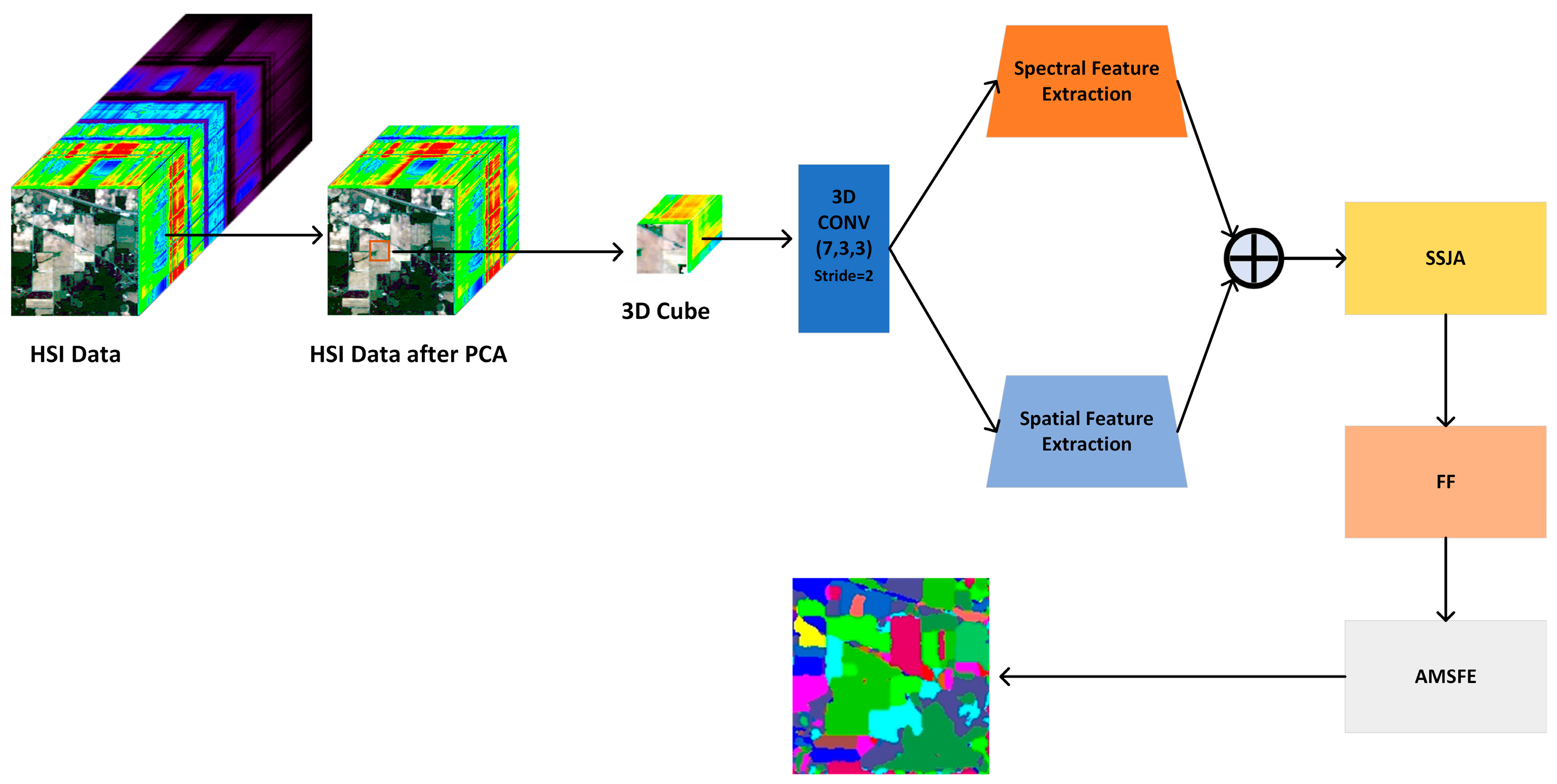
Figure 2.
The detail architecture of the proposed MSFF model.

Figure 3.
3D Convolution.

Figure 4.
3D Depthwise Separable Convolution.
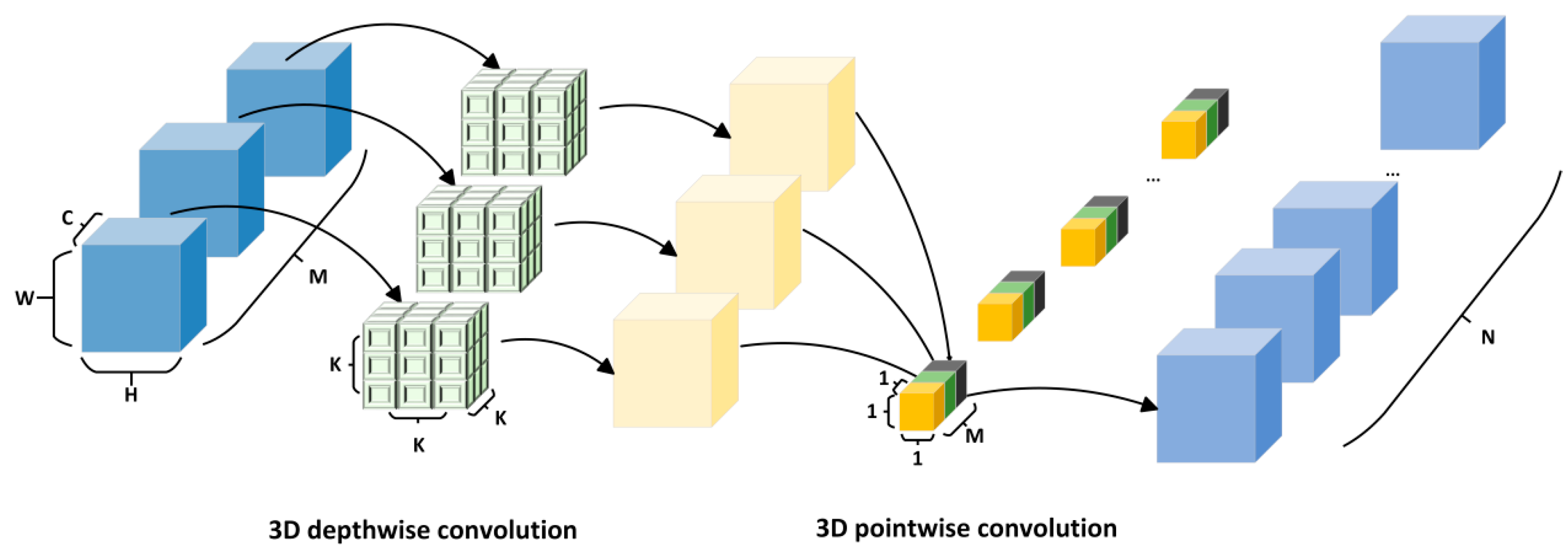
Figure 5.
The proposed ACP structure.
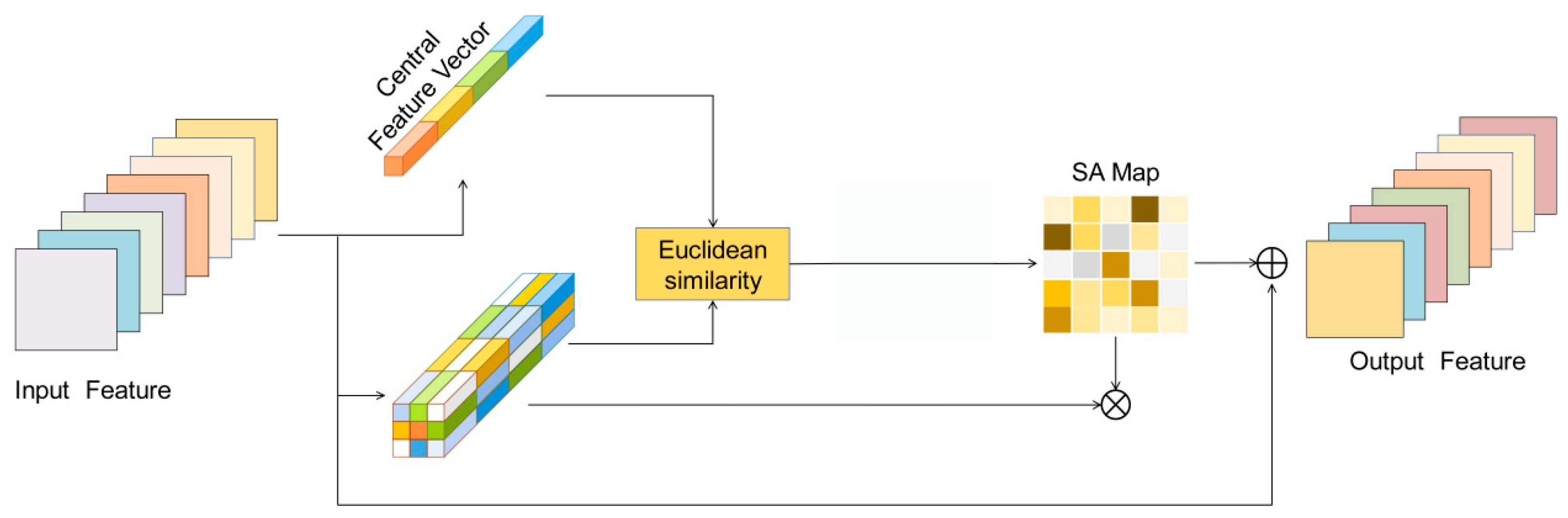
Figure 6.
Structure of spectral and spatial feature extraction module.
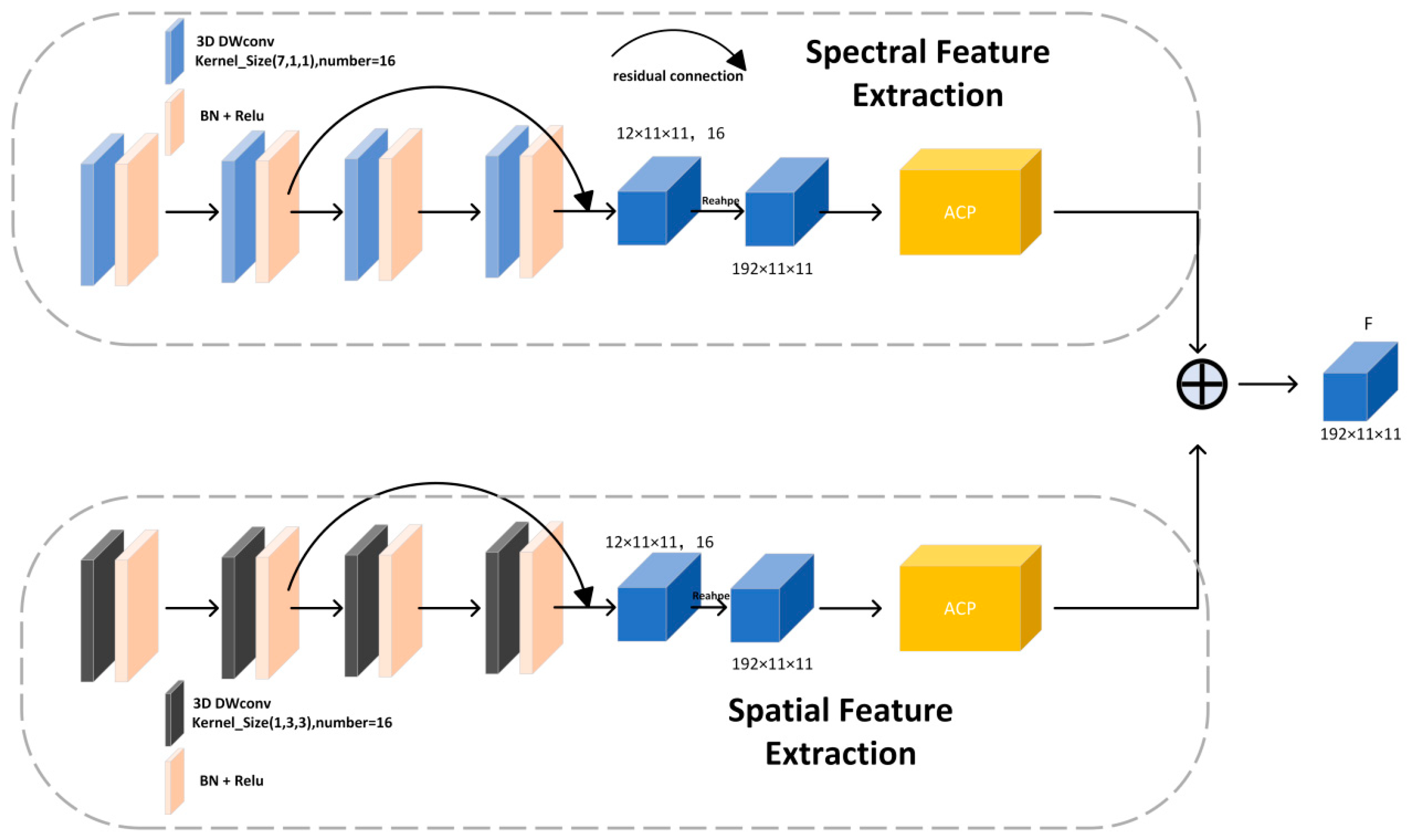
Figure 8.
The proposed FF structure.
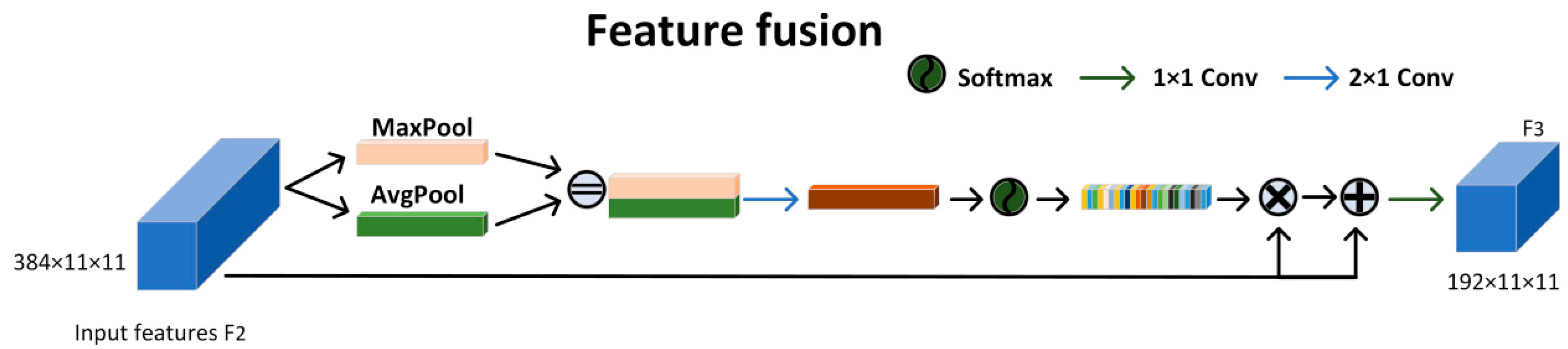
Figure 9.
The proposed NAM structure.
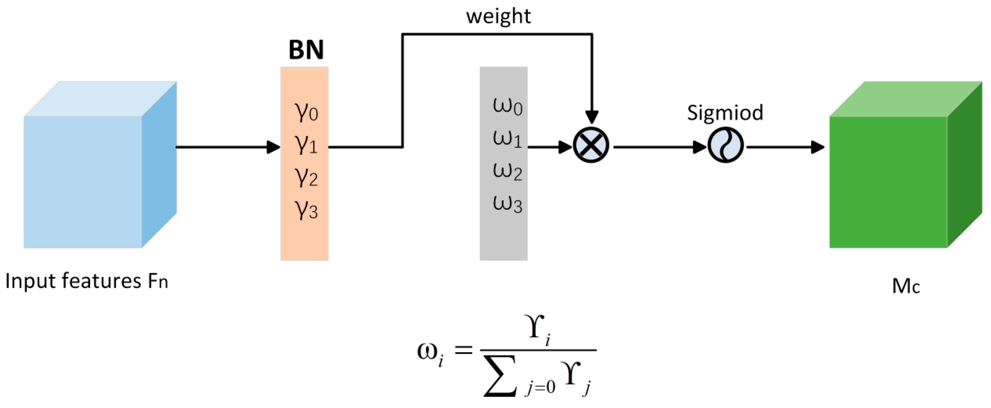
Figure 10.
The proposed AMSFE structure.
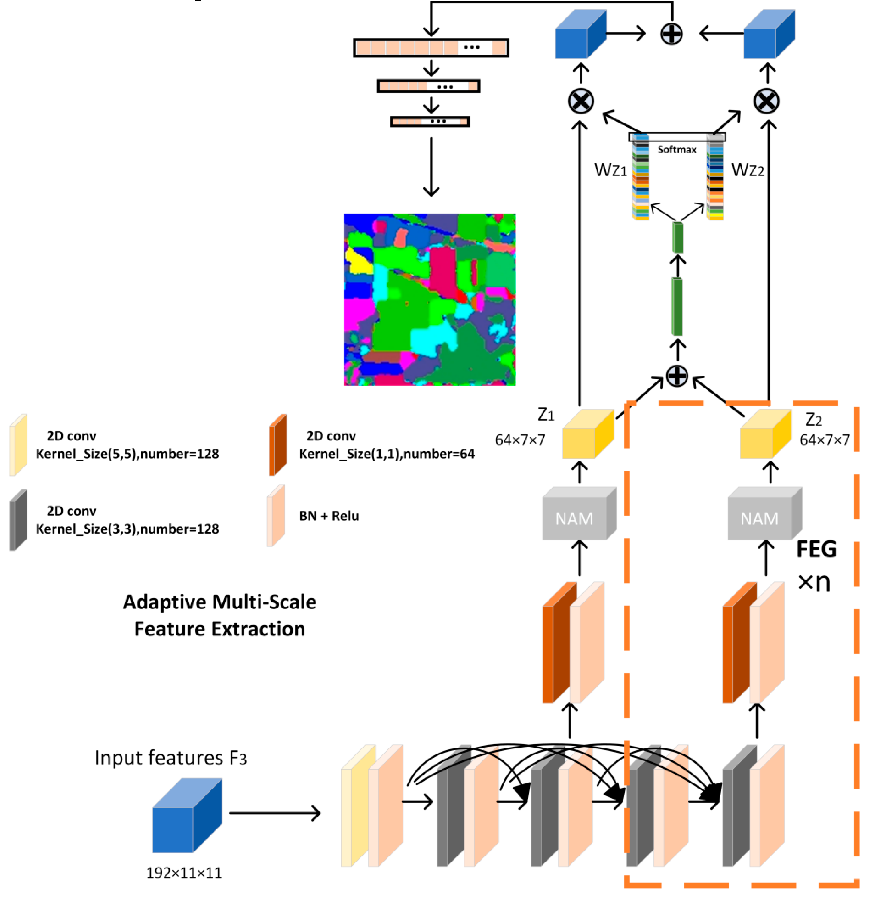
Figure 11.
Datasets and ground truth classification. (a,b) Indian Pines dataset, (c,d) Pavia University dataset, (e,f) Yellow River Estuary coastal wetland.
Figure 11.
Datasets and ground truth classification. (a,b) Indian Pines dataset, (c,d) Pavia University dataset, (e,f) Yellow River Estuary coastal wetland.
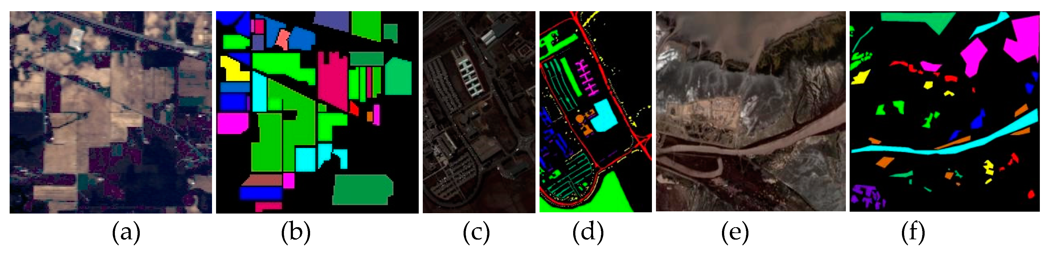
Figure 12.
The quantitative results of different batchsizes on OA,AA,and Kappa.
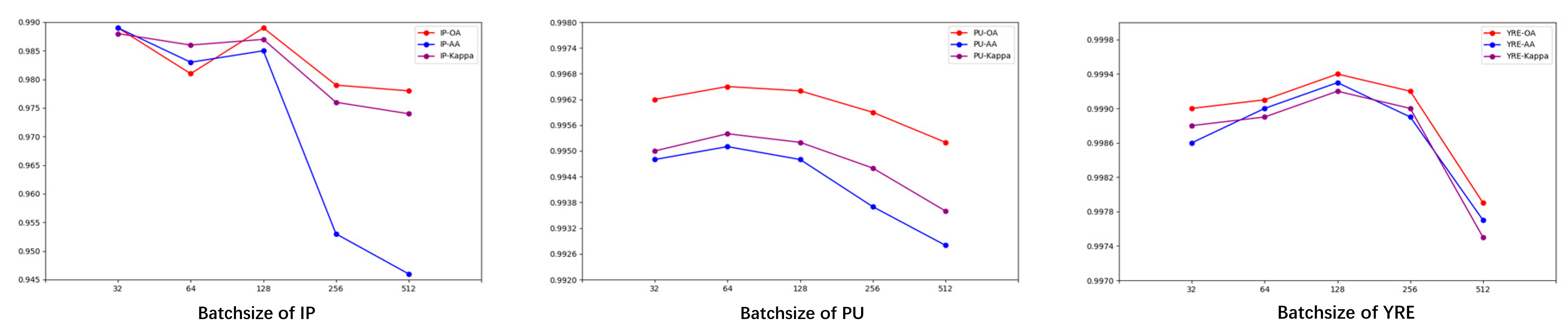
Figure 13.
The quantitative results of different patchsizes on OA,AA,and Kappa.
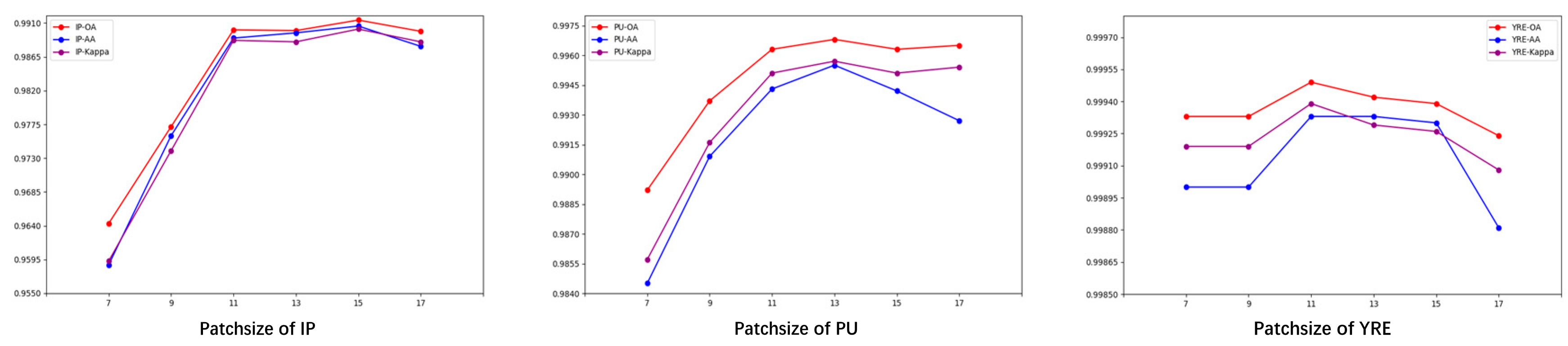
Figure 14.
The quantitative results of different channel numbers on OA,AA,and Kappa.
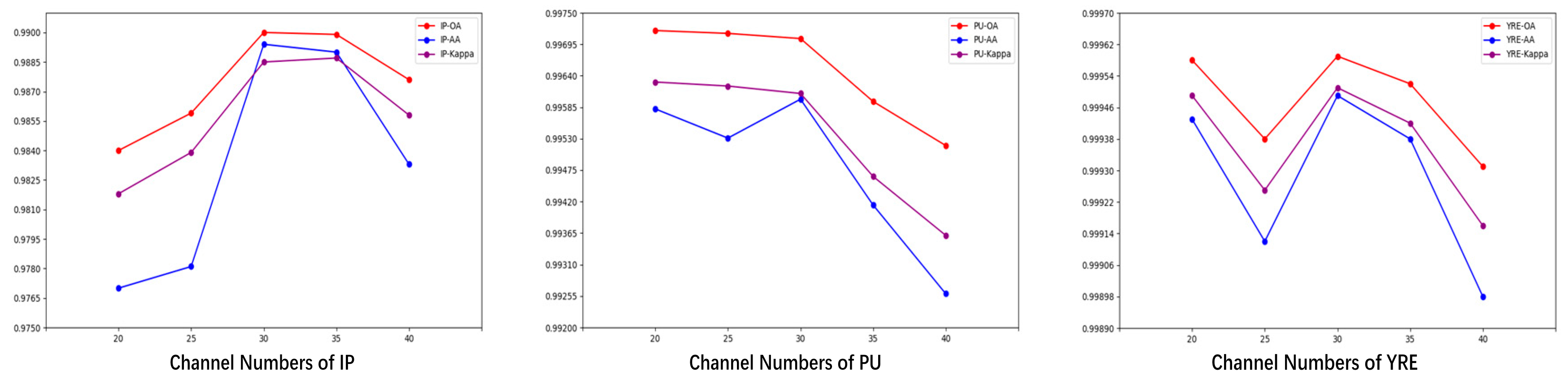
Figure 15.
The quantitative results of different FEG numbers on OA,AA,and Kappa.
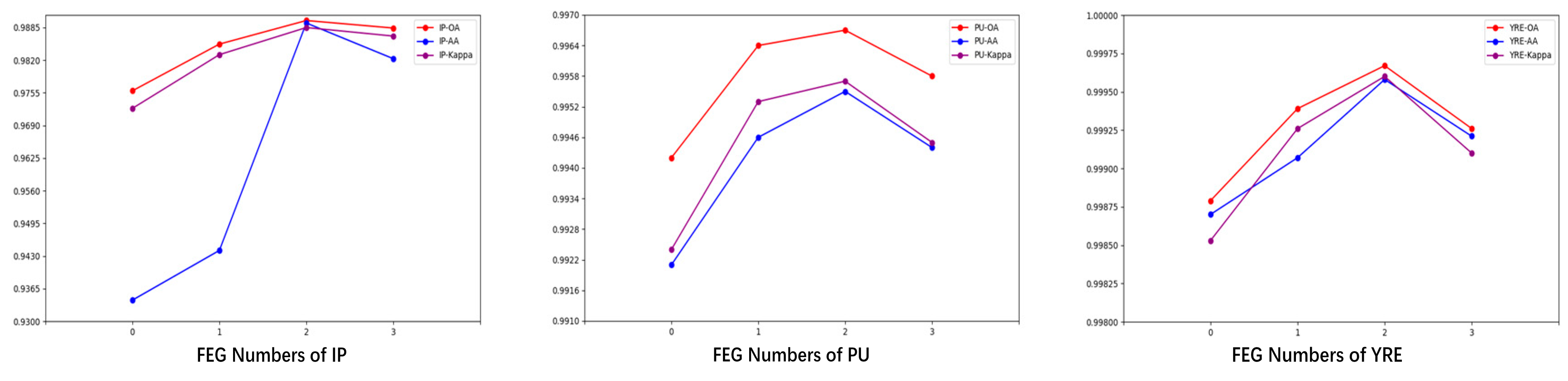
Figure 16.
Classification maps for the IP dataset. (a)Ground-truth map. (b)2D-CNN. (c)DBMA. (d)SSRN. (e) HybridSN. (f)MDRD-Net. (g)SSTFF. (h)DMAN. (i)MSFF-CBAM. (j)MSFF.
Figure 16.
Classification maps for the IP dataset. (a)Ground-truth map. (b)2D-CNN. (c)DBMA. (d)SSRN. (e) HybridSN. (f)MDRD-Net. (g)SSTFF. (h)DMAN. (i)MSFF-CBAM. (j)MSFF.
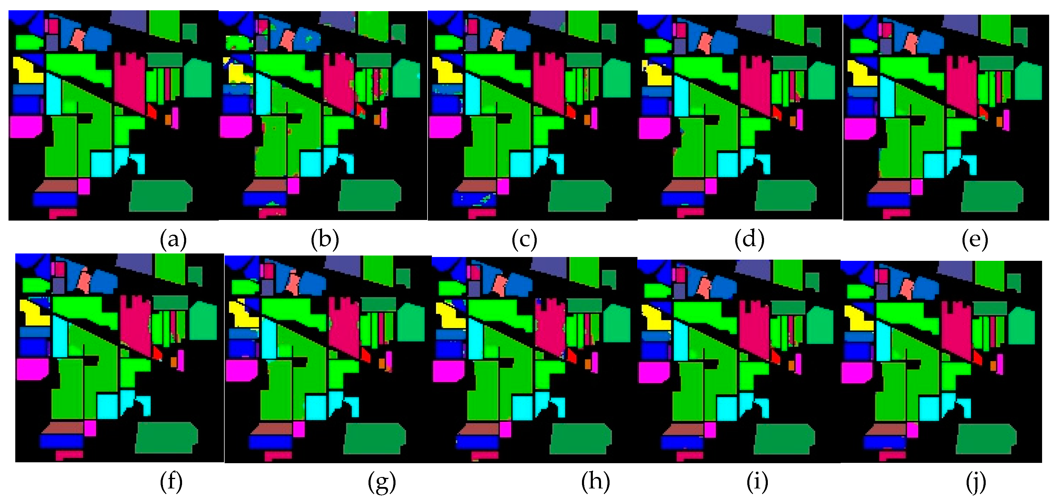
Figure 17.
Classification maps for the PU dataset. (a)Ground-truth map. (b)2D-CNN. (c)DBMA. (d)SSRN. (e) HybridSN. (f)MDRD-Net. (g)SSTFF. (h)DMAN. (i)MSFF-CBAM. (j)MSFF.
Figure 17.
Classification maps for the PU dataset. (a)Ground-truth map. (b)2D-CNN. (c)DBMA. (d)SSRN. (e) HybridSN. (f)MDRD-Net. (g)SSTFF. (h)DMAN. (i)MSFF-CBAM. (j)MSFF.
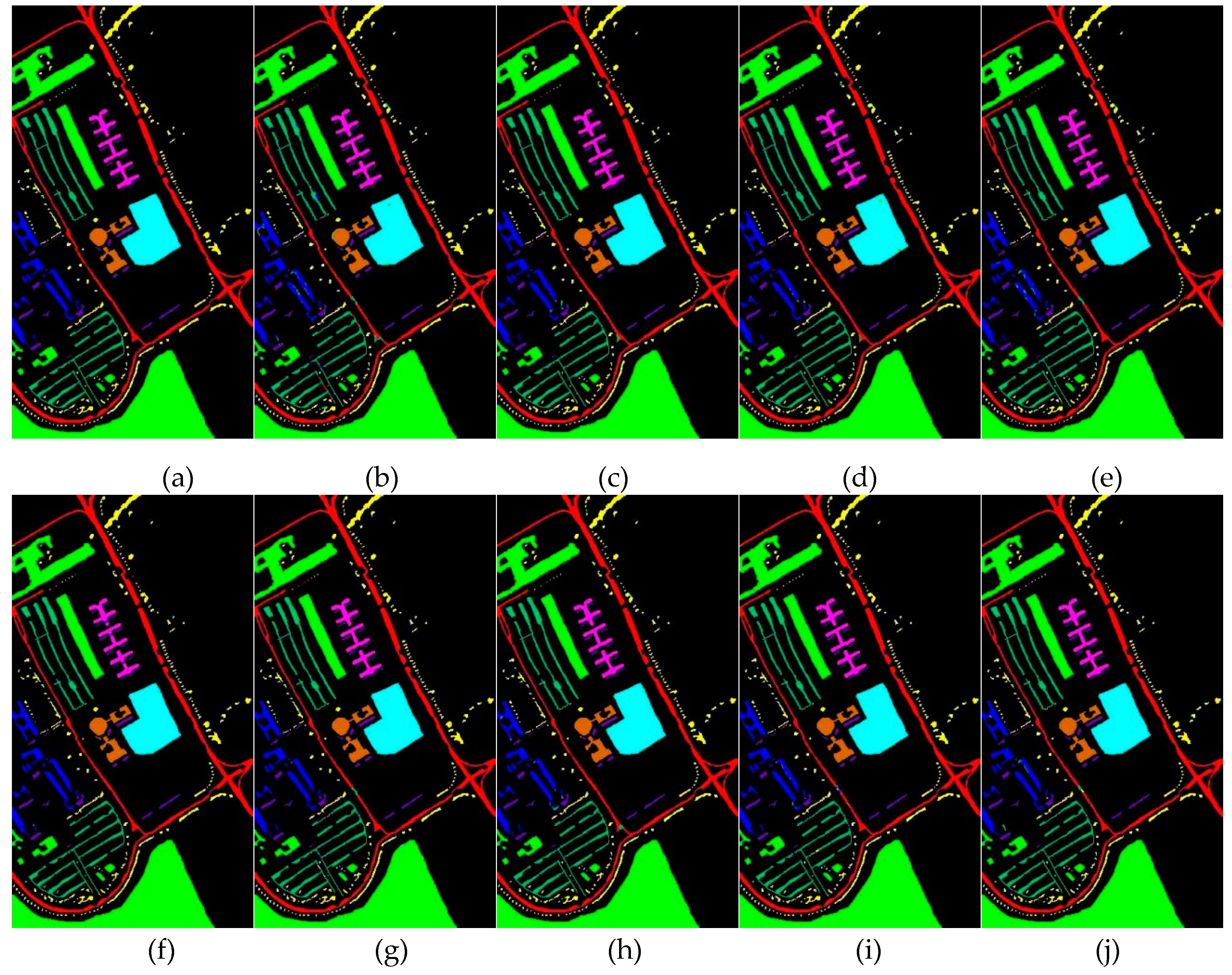
Figure 18.
Classification maps for the YRE dataset. (a)Ground-truth map. (b)2D-CNN. (c)DBMA. (d)SSRN. (e) HybridSN. (f)MDRD-Net. (g)SSTFF. (h)DMAN. (i)MSFF-CBAM. (j)MSFF.
Figure 18.
Classification maps for the YRE dataset. (a)Ground-truth map. (b)2D-CNN. (c)DBMA. (d)SSRN. (e) HybridSN. (f)MDRD-Net. (g)SSTFF. (h)DMAN. (i)MSFF-CBAM. (j)MSFF.
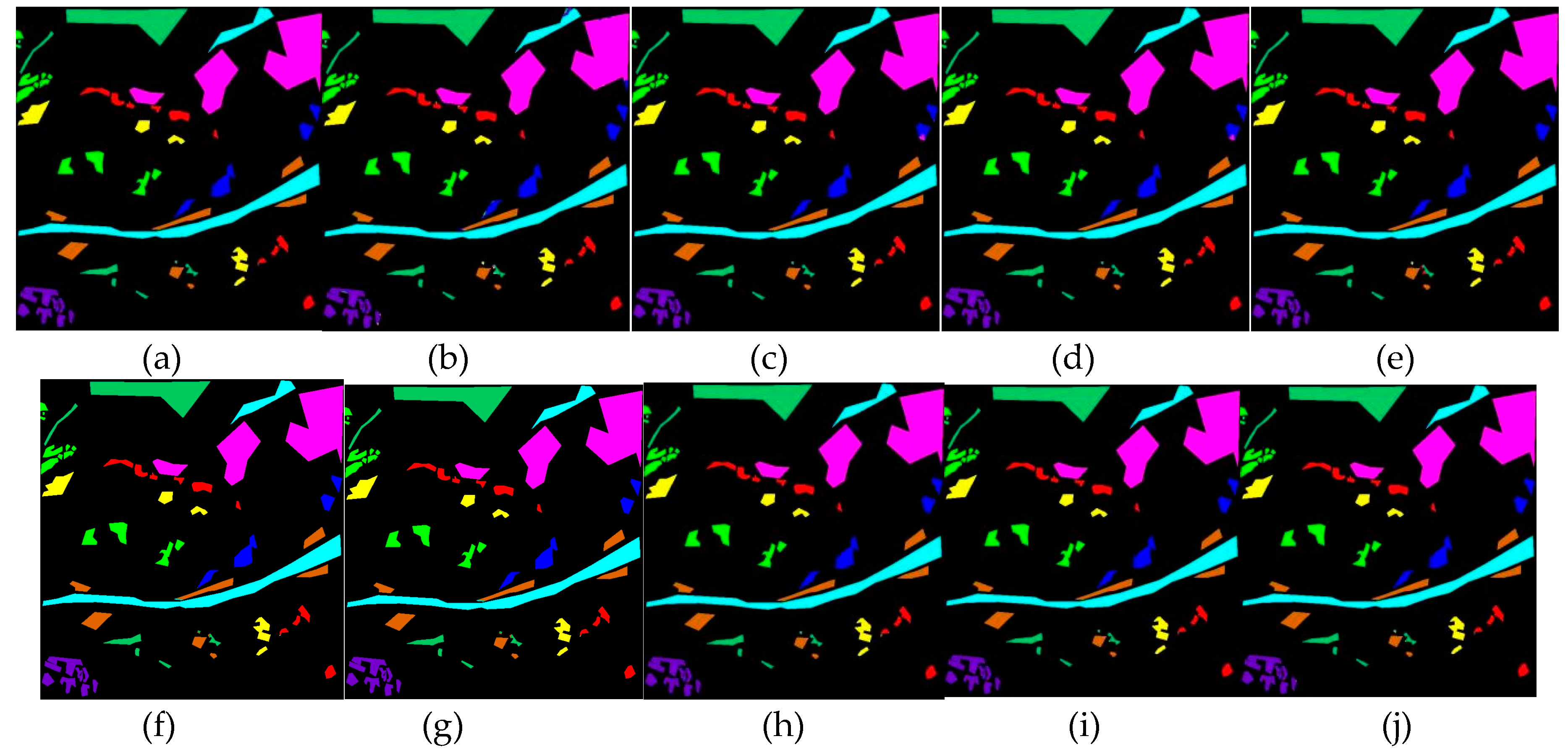
Figure 19.
The OA of various combinations in three datasets.
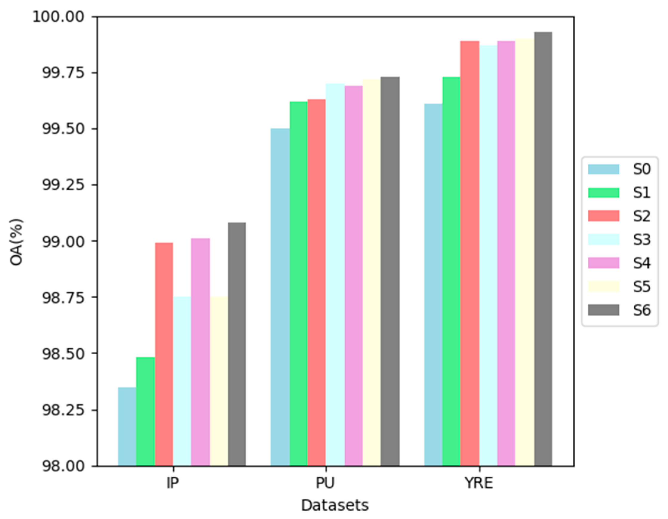

Table 1.
Indian Pines dataset categories
| Category | Class Name | Color | Sample |
|---|---|---|---|
| 1 | Alfalfa |  |
46 |
| 2 | Corn-notill |  |
1428 |
| 3 | Corn-mintill |  |
830 |
| 4 | Corn |  |
237 |
| 5 | Grass-pasture |  |
483 |
| 6 | Grass-trees |  |
730 |
| 7 | Grass-pasture-mowed |  |
28 |
| 8 | Hay-windrowed |  |
478 |
| 9 | Oats |  |
20 |
| 10 | Soybean-notill |  |
972 |
| 11 | Soybean-mintill |  |
2455 |
| 12 | Soybean-clean |  |
593 |
| 13 | Wheat |  |
205 |
| 14 | Woods |  |
1265 |
| 15 | Buildings-Grass-Trees-Drives |  |
386 |
| 16 | Stone-Steel-Towers |  |
93 |
Table 2.
Pavia University dataset categories
| Category | Class Name | Color | Sample |
|---|---|---|---|
| 1 | Asphalt |  |
6631 |
| 2 | Meadows |  |
18649 |
| 3 | Gravel |  |
2099 |
| 4 | Trees |  |
3064 |
| 5 | Painted metal sheets |  |
1345 |
| 6 | Bare soil |  |
5029 |
| 7 | Bitumen |  |
1330 |
| 8 | Self-blocking bricks |  |
3682 |
| 9 | Shadows |  |
947 |
Table 3.
Yellow River Estuary coastal wetland dataset categories
| Category | Class Name | Color | Sample |
|---|---|---|---|
| 1 | Mudflat |  |
3583 |
| 2 | Bare soil |  |
5386 |
| 3 | Tamarix |  |
3582 |
| 4 | Suaeda salsa |  |
4243 |
| 5 | Spartina alterniflora |  |
23535 |
| 6 | Turbid water |  |
17018 |
| 7 | Tidal flat reed |  |
5987 |
| 8 | Clear water |  |
12253 |
| 9 | Bare lake beach |  |
4145 |
Table 4.
Optimal hyperparameter settings for different datasets
| Datasets | Learning Rate | Epochs | Batchsize | Patchsize | Channel Number | FEG Number |
|---|---|---|---|---|---|---|
| IP | 0.0001 | 150 | 32 | 15 | 30 | 2 |
| PU | 0.0001 | 150 | 64 | 13 | 20 | 2 |
| YRE | 0.0001 | 150 | 128 | 11 | 30 | 2 |
Table 5.
The classification results (%) of all compared methods on the IP dataset.
| Classes | 2D-CNN | DBMA | SSRN | HybridSN | MDRD- Net |
SSTFF | DMAN | MSFF- CBAM |
MSFF |
|---|---|---|---|---|---|---|---|---|---|
| 1 | 100 | 100 | 100 | 100 | 100 | 100 | 97.50 | 91.67 | 97.87 |
| 2 | 91.34 | 99.14 | 99.57 | 99.64 | 96.89 | 98.06 | 97.01 | 99.13 | 100 |
| 3 | 31.53 | 95.71 | 97.63 | 98.46 | 98.91 | 98.76 | 97.15 | 97.75 | 99.64 |
| 4 | 95.11 | 100 | 99.11 | 100 | 100 | 89.38 | 94.76 | 98.33 | 99.58 |
| 5 | 97.48 | 99.57 | 99.79 | 99.79 | 99.18 | 98.57 | 99.51 | 99.79 | 99.79 |
| 6 | 97.69 | 98.91 | 99.86 | 99.59 | 98.51 | 96.58 | 99.52 | 100 | 99.45 |
| 7 | 92.86 | 100 | 100 | 100 | 100 | 67.57 | 100 | 96.55 | 100 |
| 8 | 95.88 | 100 | 99.38 | 97.55 | 100 | 100 | 100 | 99.58 | 100 |
| 9 | 91.67 | 100 | 100 | 100 | 100 | 94.74 | 93.75 | 90.91 | 94.74 |
| 10 | 92.56 | 99.67 | 97.57 | 98.88 | 99.15 | 97.82 | 98.46 | 98.26 | 98.68 |
| 11 | 92.33 | 94.93 | 98.53 | 97.71 | 98.58 | 99.68 | 98.86 | 97.92 | 98 |
| 12 | 94.44 | 99.65 | 98.66 | 97.82 | 99.15 | 97.86 | 98.02 | 99.64 | 99.66 |
| 13 | 95.28 | 100 | 100 | 99.03 | 100 | 100 | 100 | 98.55 | 99.03 |
| 14 | 98.59 | 98.21 | 99.06 | 99.84 | 99.68 | 99.73 | 99.81 | 99.76 | 99.92 |
| 15 | 94.44 | 100 | 97.18 | 99.48 | 98.21 | 99.71 | 98.80 | 99.22 | 98.97 |
| 16 | 95.83 | 96.84 | 98.92 | 96.74 | 90.72 | 88.24 | 95.12 | 92.86 | 95.79 |
| OA(%) | 94.08 | 97.85 | 98.78 | 98.79 | 98.66 | 98.35 | 98.49 | 98.71 | 99.15 |
| AA(%) | 89.71 | 92.48 | 98.56 | 95.97 | 95.35 | 97.97 | 98.14 | 98.64 | 99.06 |
| Kappa(%) | 93.24 | 97.54 | 98.60 | 98.62 | 98.47 | 98.12 | 98.28 | 98.53 | 99.03 |
Table 6.
The classification results (%) of all compared methods on the PU dataset.
| Classes | 2D-CNN | DBMA | SSRN | HybridSN | MDRD- Net |
SSTFF | DMAN | MSFF- CBAM |
MSFF |
|---|---|---|---|---|---|---|---|---|---|
| 1 | 98.69 | 99.76 | 99.73 | 99.59 | 99.68 | 99.71 | 99.65 | 99.82 | 99.91 |
| 2 | 99.58 | 99.86 | 99.64 | 99.98 | 99.89 | 99.98 | 99.83 | 99.98 | 99.98 |
| 3 | 96 | 100 | 99.76 | 99.02 | 99.71 | 99.47 | 98.92 | 98.06 | 99.85 |
| 4 | 99.33 | 99.83 | 99.97 | 99.67 | 99.33 | 99.13 | 99.85 | 99.35 | 99.48 |
| 5 | 99.78 | 100 | 100 | 100 | 100 | 98.94 | 100 | 99.85 | 100 |
| 6 | 99.30 | 99.88 | 99.74 | 99.72 | 99.84 | 99.82 | 99.85 | 100 | 99.98 |
| 7 | 98.79 | 100 | 99.70 | 99.63 | 98.81 | 100 | 99.50 | 99.70 | 99.70 |
| 8 | 93.88 | 97.71 | 98.45 | 96.13 | 99.03 | 98.59 | 96.82 | 98.62 | 97.94 |
| 9 | 95.31 | 99.89 | 100 | 99.89 | 92.81 | 97.67 | 99.41 | 98.64 | 99.47 |
| OA(%) | 98.60 | 99.67 | 99.61 | 99.46 | 99.53 | 99.63 | 99.48 | 99.59 | 99.73 |
| AA(%) | 97.90 | 99.50 | 99.44 | 99.11 | 98.75 | 99.41 | 99.14 | 99.50 | 99.56 |
| Kappa(%) | 98.15 | 99.56 | 99.48 | 99.29 | 99.38 | 99.51 | 99.31 | 99.54 | 99.64 |
Table 7.
The classification results (%) of all compared methods on the YRE dataset.
| Classes | 2D-CNN | DBMA | SSRN | HybridSN | MDRD- Net |
SSTFF | DMAN | MSFF- CBAM |
MSFF |
|---|---|---|---|---|---|---|---|---|---|
| 1 | 99.19 | 99.71 | 99.64 | 97.90 | 100 | 99.89 | 99.97 | 99.92 | 99.86 |
| 2 | 99.06 | 99.98 | 99.96 | 100 | 100 | 100 | 100 | 99.96 | 100 |
| 3 | 93.99 | 99.47 | 100 | 100 | 99.97 | 99.43 | 99.46 | 100 | 100 |
| 4 | 97.56 | 99.13 | 99.88 | 99.58 | 99.91 | 99.81 | 99.76 | 99.76 | 99.51 |
| 5 | 99.89 | 98.94 | 99.52 | 100 | 99.98 | 99.90 | 99.99 | 99.99 | 100 |
| 6 | 99.94 | 99.82 | 100 | 99.96 | 99.79 | 100 | 100 | 100 | 99.98 |
| 7 | 99.98 | 100 | 100 | 100 | 99.40 | 99.74 | 99.95 | 100 | 100 |
| 8 | 99.23 | 98.59 | 100 | 99.78 | 100 | 99.83 | 99.93 | 99.65 | 99.98 |
| 9 | 96.43 | 97.67 | 100 | 99.95 | 99.95 | 100 | 100 | 99.93 | 100 |
| OA(%) | 99.12 | 99.63 | 99.83 | 99.83 | 99.89 | 99.88 | 99.94 | 99.92 | 99.96 |
| AA(%) | 99.15 | 99.41 | 99.61 | 99.84 | 99.86 | 99.82 | 99.92 | 99.90 | 99.95 |
| Kappa(%) | 98.94 | 99.51 | 99.79 | 99.80 | 99.87 | 99.85 | 99.93 | 99.90 | 99.95 |
Table 8.
The way the attention modules are combined in the model.
| Name | ACP | SSJA | FF |
|---|---|---|---|
| S0 | Without | ||
| S1 | √ | ||
| S2 | √ | ||
| S3 | √ | ||
| S4 | √ | √ | |
| S5 | √ | √ | |
| S6 | √ | √ | |
Disclaimer/Publisher’s Note: The statements, opinions and data contained in all publications are solely those of the individual author(s) and contributor(s) and not of MDPI and/or the editor(s). MDPI and/or the editor(s) disclaim responsibility for any injury to people or property resulting from any ideas, methods, instructions or products referred to in the content. |
© 2024 by the authors. Licensee MDPI, Basel, Switzerland. This article is an open access article distributed under the terms and conditions of the Creative Commons Attribution (CC BY) license (http://creativecommons.org/licenses/by/4.0/).
Copyright: This open access article is published under a Creative Commons CC BY 4.0 license, which permit the free download, distribution, and reuse, provided that the author and preprint are cited in any reuse.


