Submitted:
11 July 2023
Posted:
14 July 2023
You are already at the latest version
Abstract
This work focused on proposing a plan for improvement and control of the customer service process in a customer service center, based on a waiting line analysis where it describes all the elements that interact in the system and a statistical analysis of processes to define the state in which it operates. Subsequently, the simulation of processes is applied to represent the system studied, and with it, to be able to evaluate different strategies for improvement and increase in productivity. The following strategies were evaluated: correction of the instability of customer service processes, establishment of new specification limits according to the promise of value to be fulfilled to customers, human resource management, administrative technical support. Finally, with the results obtained from the simulation of the system, the improvement and productivity increase plan is planned according to the DMAMC (Define, Measure, Analyze, Improve, Control, or DMAIC) continuous improvement cycle established in six sigma
Keywords:
continuous improvement
; waiting line
; DMAIC
; simulation
; process control
; productivity
; customer service
Introduction
The economy of a country is made up of companies, one of them the services, which according to recent studies generates most of the GDP of nations, approximately 76%, being the fastest growing sector in the global economy of the last decade. Therefore, it is vitally important to analyze the capacity they have when it comes to meeting customer requirements. At present, companies recognize that giving good customer service generates a level of satisfaction in it, in this way they cause it to reacquire a good or service at a later time, make the company known to other potential customers.
In the last decade, several quality management strategies have been implemented, especially in the service sector. Among them, continuous improvement prevails as the most popular due to its unique ability to provide a competitive advantage to companies. (Butler et al., 2018).
Modern economies are under constant pressure and those that ensure correct negotiation in all their processes remain in the market. Corporations that can minimize waste and errors, and that possess a management philosophy that can turn mistakes into learnings for later success will be the ones that survive in the market making profits and maintaining an efficient business. The six sigma method is a project-driven management approach to improving the organization's products and services and processes. It is a business strategy that focuses on improving customer requirements, understanding, business systems, productivity, and financial performance. (Bilgen & Şen, 2012)
Six sigma tools discover the causes of potential problems and through this methodology eliminate possible defects, this means that this methodology takes action in the early stages of product or process development before the problem arises. (Taghizadegan, 2006)
Within the modalities of customer service, there are customer service systems, which consist of an arrangement of people willing to solve the questions or needs that this maintains, therefore, it is appropriate that companies worry about giving a good service through a convenient waiting time to receive attention and a timely service time to meet the expectations that the client has with the service.
One of the companies that uses this type of service is the National Telecommunications Corporation EP, by its nature of providing services, uses these customer service systems. The company has identified that the value offer is not met in terms of waiting time and customer service time in one of its centers, the level of service is less than 40% and the wait fluctuates between 5 to 56 min, therefore, it is essential to identify the causes to be attacked.
The objective of this work is to propose a plan for improvement and control of the customer service system through the application of the methodology of waiting line analysis and scheduling of operations with emphasis on reducing waiting times, improving the level of service and increasing productivity.
To achieve this objective, the following route was proposed: to carry out an analysis of the current situation of the waiting line of the customer service system according to waiting times, times and level of service, to apply the waiting line simulation to develop a model of study of the current state of the service system, Through the simulated process, evaluate the different strategies for improvement and increase in productivity, and propose a plan for improvement and control of the care system according to the results of the improvement strategies.
2. Theoretical Framework
Before referring to customer service systems, it is necessary to understand what it means to serve the customer?, (Ariza and Ariza, 2017) mention that customer service is a set of procedures coordinated by the company where the customer-company relationship is managed by promoting customer satisfaction, therefore, Customer service is always focused on seeking to meet the needs of the customer and for this the company has resources, whether physical, human, infrastructure, etc. This gives rise to customer service systems. Therefore, a customer service system is understood as the set of physical facilities and human resources in order to quickly meet the needs of customers and thereby generate satisfaction and loyalty to the company.
2.1. Waiting Line Analysis
In the day to day, the waiting lines are present at all times, either in the circulation of vehicles waiting for a traffic light to change the signal to green, even in all financial institutions waiting lines are formed for customers eager to make some type of transaction, however, not because they are common, they stop presenting inconveniences to the organizations that have them, this can cause losses in time, money, even human if the waiting line in a hospital is too long (Chase and Jacobs, 2009).
The waiting line analysis consists of the study of:
- Disposition and distribution of arrival of customers
- Provision of resources to provide the service
2.1.1. Disposition and distribution of arrival of customers
In the study of customer arrival, it is necessary to specify the origin of customers: a finite population (for example in doctors' offices, the demand for patients is fixed and there is no possibility of serving more) or infinite (for example in financial institutions, the successive arrival of customers), this will define the law of probability to be used in the distribution of the arrival and estimation of customer demand.
The arrival distribution refers to the speed or rate at which customers approach the system requiring a service, however, to conduct a study of the arrival of customers, it is necessary to differentiate the arrival times of customers and the time between arrivals.
Figure 1.
Time of arrival and time between arrivals.
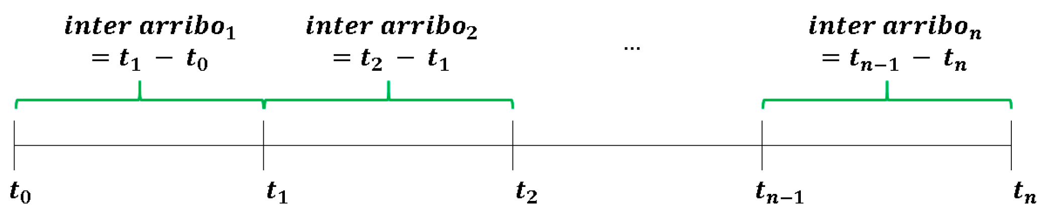
The time of arrival corresponds to the moment of arrival), on the other hand, the inter arrival times correspond to the width of the interval.
For the estimation of customer demand, it is necessary to apply the Poisson Process or counting, which represents the number of events (customer arrivals) that can be generated in a time interval (Evans et al., 2005). For the application of this probabilistic model it is necessary to meet the following conditions:
- The arrival of customers is independent of each other
- The arrival of customers has to be one at a time, and the probability of 2 or more arriving is zero.
- The number of customers arriving in one time interval is independent of the number of customers arriving in another time interval
With the fulfillment of these conditions, the time between customer arrivals follows an exponential distribution (with parameter). (Lantz & Rosén, 2017)
And the arrival rate of customers follows a Poisson distribution (with parameter ). (Ross, 2019)
2.1.2. Provision of resources to provide the service
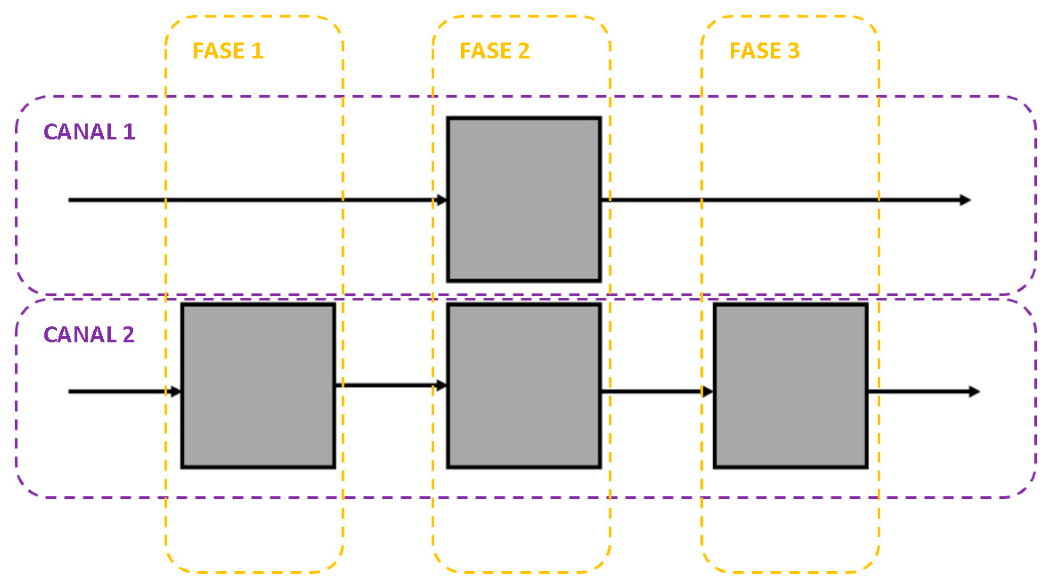
Within the analysis of the waiting line, the speed of customer service must be taken into account, this can be constant or variable. Waiting lines are configured in such a way that they can include multiple servers, in a phased and channel flow design (Chase and Jacobs, 2009).
The most commonly used configuration is multiple channels with multiple phases; This arrangement includes consecutive servers, and multiple wait lines.
Figure 2.
Configuration multiple channels and multiple phases.
To solve this type of problem, there are equations developed for some configurations (Chase and Jacobs, 2009), however, for more complex systems, where different processes are involved, therefore, different times, different customer demands, a variable number of servers, etc., the simulation of the waiting line is used.
2.2. Waiting Line Simulation
Wait-line simulation combines probabilistic models (e.g., exponential distribution), and statistical functions (e.g., minimum, maximum, medians) to represent the randomness and characteristics under which the system works. This tool monitors the occurrence of events of interest and the flow resulting from the system's own interactions through the analysis of random variables. (Ross, 2019)
Given the complexity of these models due to the interactions they imply, in the present work it uses the JAAMSIM® software which is programmed to carry out this type of studies and offers certain advantages over other types of software (JaamSim Development Team, 2014).
2.3. Statistical Process Control
The statistical control of processes is a tool for the management of quality in the company, through control graphics the representation of the limits is made (either specification, or control), and which serve as a guide to control the evolution of the performance of a system (Pulido, 2003).
The control limits correspond to the following:
For the :
Where:
: is the average of the averages of the samples taken
: replacement factor
: is the average of the ranges of the samples taken
For the :
: factor for the upper control limit
: factor for the lower control limit
To finish with the diagnosis, monitoring and control of the operation of the system, it is essential to use the process capacity indexes, which allow us to conclude on the ability of a process to comply with a specific quality level and identify possible improvements (Gutiérrez, 2010).
Where:
: potential capacity index
: lower capacity index
: Superior capacity index
: Process centering index
: Taguchi index
: upper specification limit
: lower specification limit
: average or average
:standard deviation
2.4. Improvement plan
The quality of a service, is not a matter of a short-term goal, much less of establishing a plan and not implementing it, quality is done day by day, with a comprehensive commitment that links from the management to the advisors and people involved in giving a service that satisfies the client,
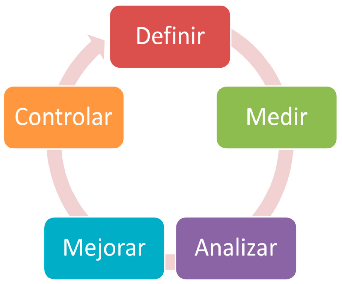
For the realization of an improvement plan, you can choose several methodologies, among them is the methodology or also known as a clear and easy to implement DMAIC roadmap to improve the processes extracted from the six sigma tools. (Zhang et al., 2015).
This methodology establishes a way forward, and the application of the stages of the cycle will allow the obtaining of benefits as long as the problem or root cause is correctly defined (Gupta and Sri, 2016).
Figure 3.
Six sigma continuous improvement cycle (DMAMC or DMAIC).
3. Results and Discussion
3.1. Description of the Waiting Line
The analysis was applied to the behavior of the customer service system offered by a telecommunications company, in one of its service centers. The problems presented correspond to the lack of fulfillment of its value proposition when delivering a service, a low level of service and a long waiting time.
This center operates from Monday to Friday and its opening is at 8:00, and closing at 18:30. The center works around 10.50 h for 5 days a week, there is no attention on weekends and the hours of operation are uninterrupted at noon.
Figure 4.
Customer Service Center Layout.
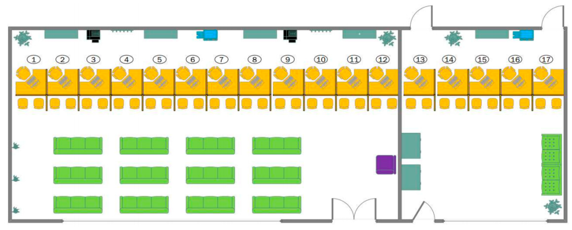
The center consists of:
- Seventeen customer service stations (marked in yellow), where customers come to meet their requirements.
- Forty seats (marked in green), where customers are kept expectant of their turn to approach the designated service module.
- A reception station (marked in purple) and shift generation depending on the type of requirement that will be attended.
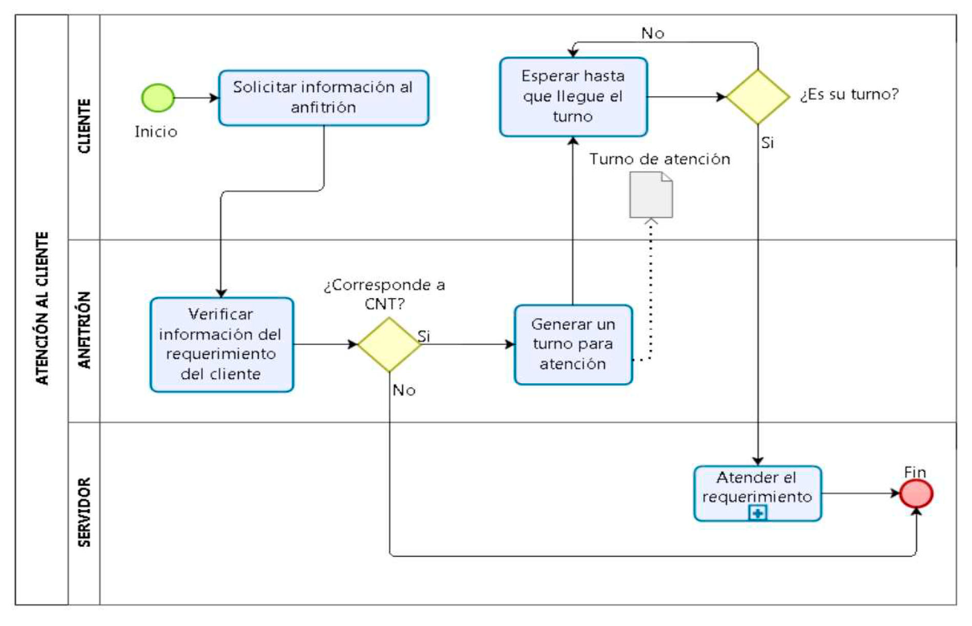
And, the process applied is:
Figure 4.
Customer Service Process.
3.2. Waiting Line Analysis
For the present analysis, the records from the years 2015, 2016 and 2017 were considered, because it can be assumed that the behavior of customers in search of the service is maintained in recent years. Giving a total of 395 962 cases analyzed.
3.2.1. Study of customer arrival
For the analysis, it was necessary to identify the strange data, those that are not due to a normal behavior corresponding to the arrival of customers to the service system, these data were excluded since they generated erroneous estimates and inconveniences in the simulation of the system.
It is common for this atypical data to be presented, this system works in real life and is subject to uncontrollable variables. In Figure 5, the black dots correspond to the atypical data, which were not taken into account in the analysis of descriptive statistics.
Figure 5.
Box and whisker diagrams for the analysis period by years.
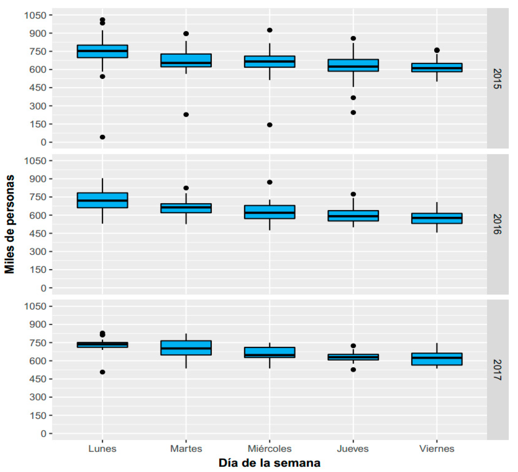

Table 1.
Descriptive statistics of daily care.
| Day | Min | Max | Stocking | Standard deviation |
|---|---|---|---|---|
| Monday | 570 | 924 | 737 | 70 |
| Tuesday | 526 | 836 | 674 | 69 |
| Wednesday | 475 | 817 | 645 | 69 |
| Thursday | 456 | 783 | 617 | 63 |
| Friday | 456 | 762 | 601 | 66 |
The demand for the care service is differentiated per day, in addition, on Mondays an average of 737 attentions are experienced, while on Fridays, the average number of people attended is 601. To standardize the arrival rate between days, it is calculated by:
The database obtained, refers to the following data collection, the system opened its doors at 8h 00min 00s and the last client arrived at 18h 2min 37s, the operating time on that day was equal to 10 h, 2 min and 37 s or, 602, 62 min. And when considering that, on the same day 684 people were attended, it is obtained that the arrival rate is . By applying this procedure it was obtained:
Table 2.
Arrival fees.
| Day | Media | Standard deviation |
|---|---|---|
| Monday | 0,857 | 0,100 |
| Tuesday | 0,946 | 0,192 |
| Wednesday | 1,001 | 0,335 |
| Thursday | 1,005 | 0,109 |
| Friday | 1,048 | 0,116 |
Subsequently, the distribution function of customer arrival was identified, which was applied to represent this phenomenon.
Figure 6 shows that the distributions that most closely approximate the real data generated by the arrival of customers are the gamma distribution and the normal, the exponential is totally deviated. To avoid subjectivity in choosing the distribution, the goodness-of-fit test was applied (Montgomery and Runger, 2003). By means of the tests of Kolmogorov Smirnov the following results were obtained:
Figure 6.
Distribution of arrival time – Monday.
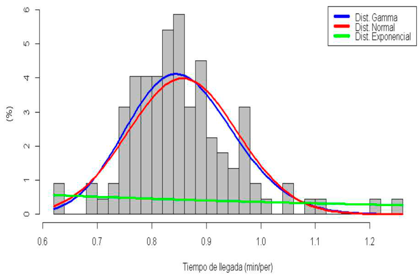
Table 3.
Goodness of fit test – Monday.
| Distribution | E(x) | Where(x) | p-value | Conclusion |
|---|---|---|---|---|
| Exponential | 0,857 | 0,100 | 0,000 | Rejected |
| Gamma | 1,005 | 0,109 | 0,486 | Accepted |
| Normal | 1,048 | 0,116 | 0,386 | Accepted |
The gamma and normal distribution can be used to represent the arrival rate on Mondays (it is accepted that they come from these distributions), in this case, it is preferable to use the gamma distribution. The same procedure was applied for the rest of the days. The arrival rates served by the care center follow a gamma distribution with the following parameters.
Table 4.
Goodness of fit test – Monday.
| Day | E(x) | Where(x) |
|---|---|---|
| Monday | 0,857 | 0,010 |
| Tuesday | 0,930 | 0,009 |
| Wednesday | 0,972 | 0,012 |
| Thursday | 1,004 | 0,011 |
| Friday | 1,047 | 0,013 |
3.2.2. Study of customer service
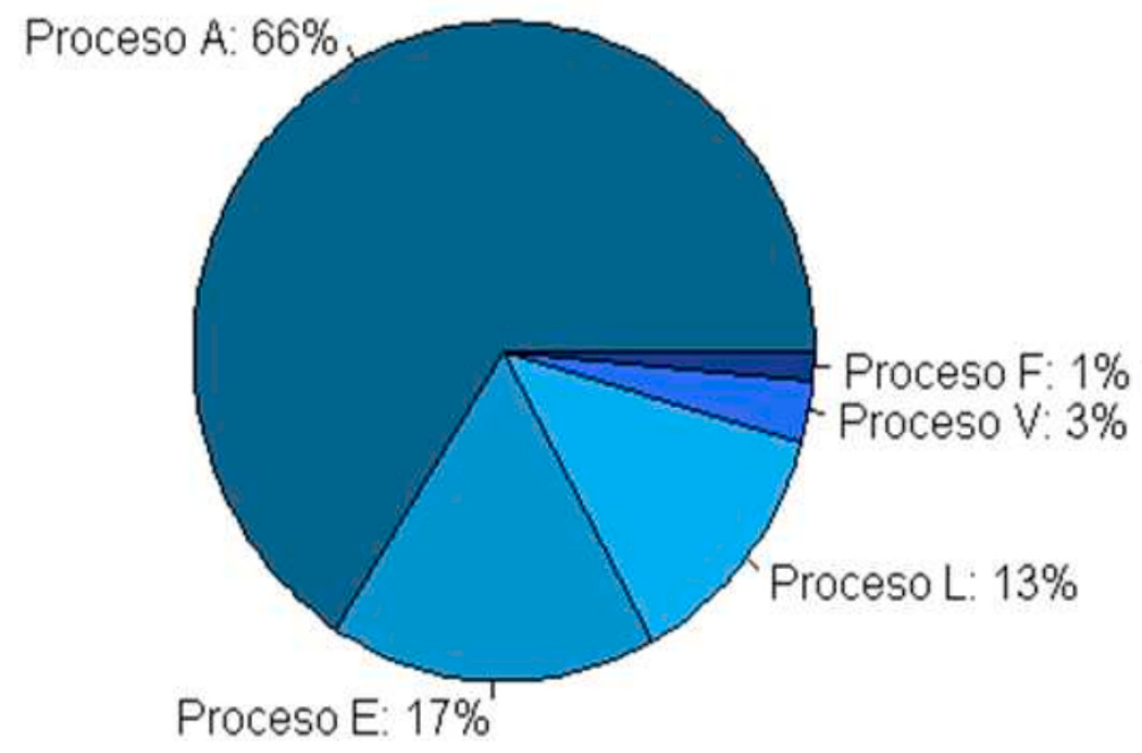
For the study of the distribution of customer service time, there was a need to identify the processes that are carried out, the 395 962 clients were served under the following scheme.
Figure 7.
Proportion of care by process.
To continue, there was a need to determine how long the servers are delayed in each of the procedures performed, for this the analysis of descriptive statistics was applied, with which it was obtained.
Table 5.
Descriptive statistics by care process.
| Process | Min | Max | Media | Standard deviation |
|---|---|---|---|---|
| A | 0,02 | 26,85 | 7,46 | 6,35 |
| And | 0,02 | 26,77 | 7,90 | 6,21 |
| F | 0,03 | 12,18 | 3,60 | 2,73 |
| L | 0,02 | 32,97 | 9,18 | 7,76 |
| In | 0,02 | 32,37 | 8,33 | 7,77 |
Once the procedure was applied to estimate the distributions of attention times, it was found that no distribution adjusts to the behavior in the attention of each of the processes. We considered 32 distributions with the EasyFit® software, and none were functional, therefore, to identify the behavior of the attention time for each of the processes, the control letters were applied. The processes analyzed are of the massive type, therefore the tools to be applied correspond to the control letters. With which the following control letters were obtained.
Figure 7.
Control letter for process A
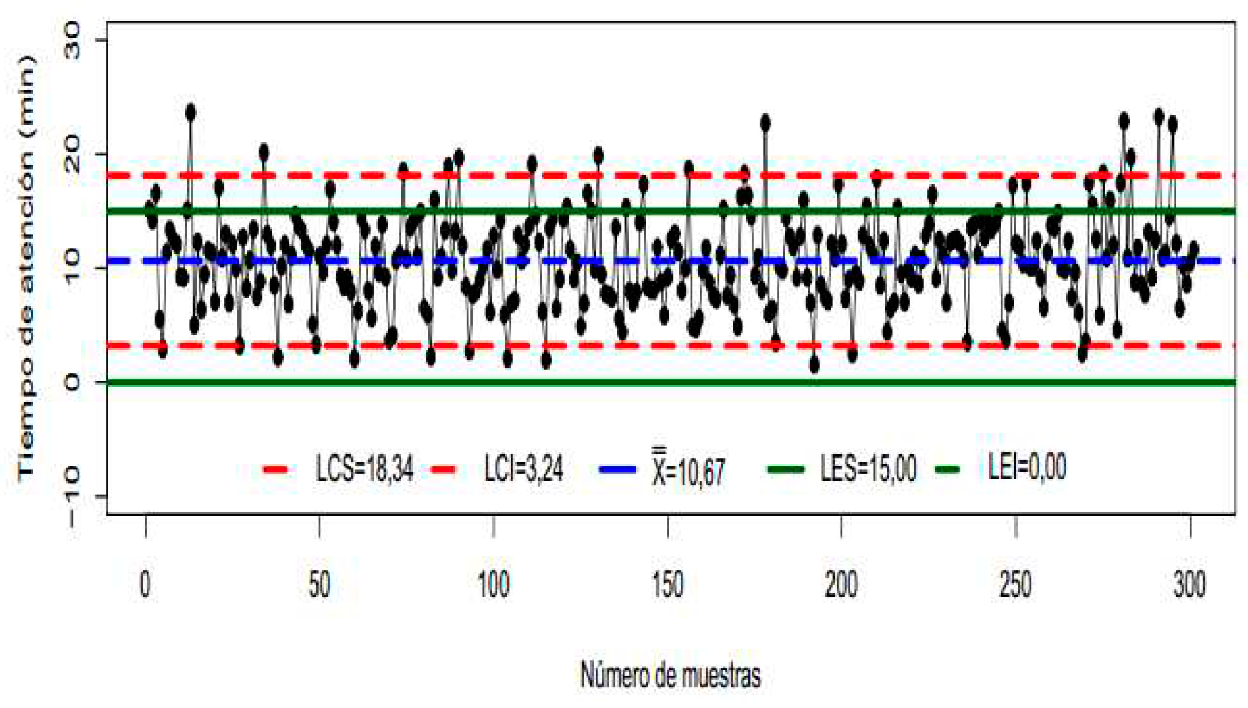
Figure 7.
Control letter for process A .
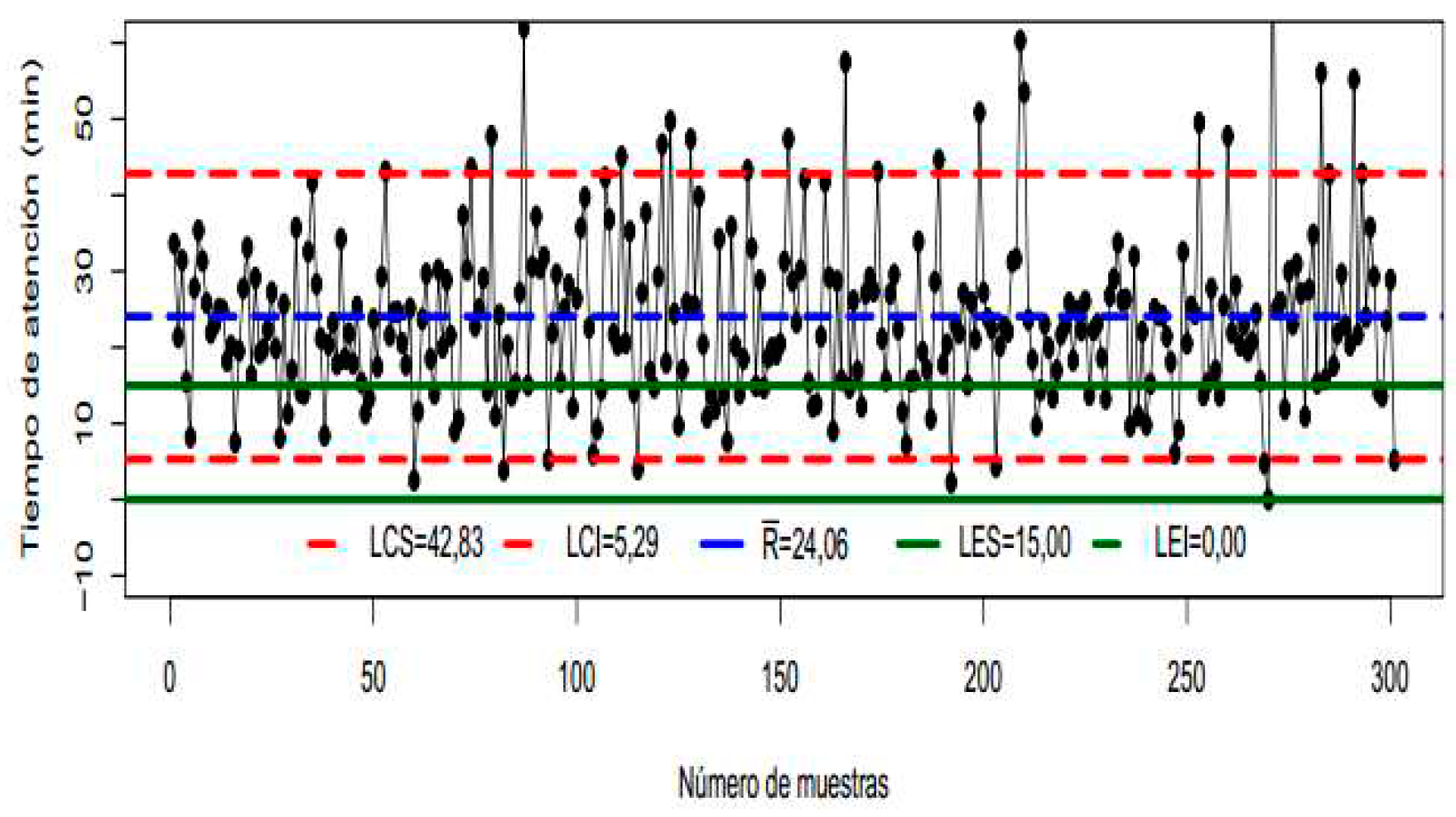
In the control letters it was observed that the attention process (any of them) is in imbalance, the control limits established by the processes are higher than the specification limits, in addition, it is common to observe points outside the specification limits. As for the ranges, an important distortion is seen since instead of reducing the ranges under which the attention times appear, it was possible to review that they are expanded, with this, the increase in the variability of the process was demonstrated.
For process F, no observations were obtained during the last year, because, as of 2017, the shifts that were attended with process F, are now attended in process A. To finalize the diagnosis, the process capability indices were applied. With which the following results were obtained:
Considering the index, it can be observed that the variation of the processes is too high with reference to the range of the specification limits, with an average of , the processes are not able to meet the specifications. As for the real capacity index, which takes into account the position, it was possible to see that there is a greater capacity in relation to the lower limit, and for the upper limit the capacity of this process is much lower, that is, most of the time, the observations were above the upper limit, He also shows that apart from the fact that the processes are not capable, they are off-center with a tendency to be outside the upper limit. As for the index, evaluates how centered the processes are, with respect to the interval defined by the specification limits, the observed values (> 20%), it was possible to confirm that the processes are off-center. The previous indicators, at least consider intervals for their calculation, unlike the Taguchi index, this is much more acid in terms of evaluating what the processes are capable of, and the values obtained showed a very poor performance, since the variation they have is too large to meet the value offer of the company.
3.3. Simulation of the customer service system
Through a simulation model built in JAAMSIM, the behavior of the demand that the care system perceives daily was incorporated, the attention time according to the applied process,® and the disposition of both physical and human resources and the disposition of the waiting line.
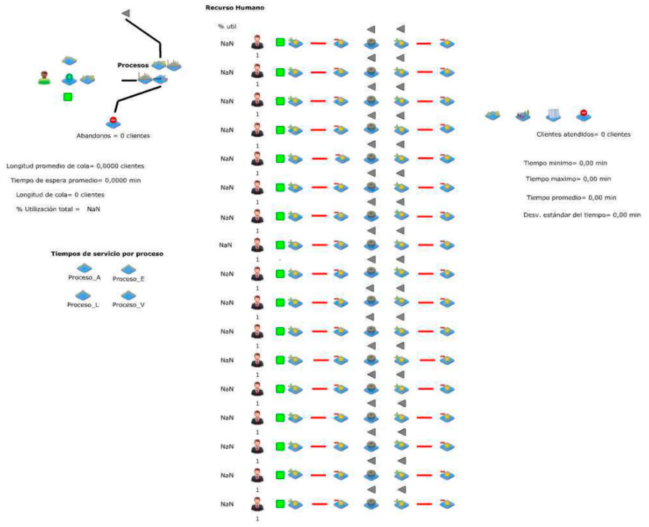
Figure 8.
Simulated workstation.

- Corresponds to the representation of the human resource assigned to attend at the workstation
- It is an indicator of availability of care, if the indicator marks a green color, then the station and a server are available to serve a client
- These objects tied together, perform the operation of taking the client, the station and the server, this set must be complete so that customer service can be performed
- In this object the customer service process is carried out
- These objects release the set formed before the customer service operation, the client is released after being served, the station and server are available to serve another client
- these objects are representations of internal queues although the client does not queue at the workstation in real life these objects are necessary for the simulation model to function correctly
Figure 8.
Representation of the system using a simulation model.
To validate the operation, the absolute error rates were verified.
Figure 9.
Absolute error rates between observed and simulated.
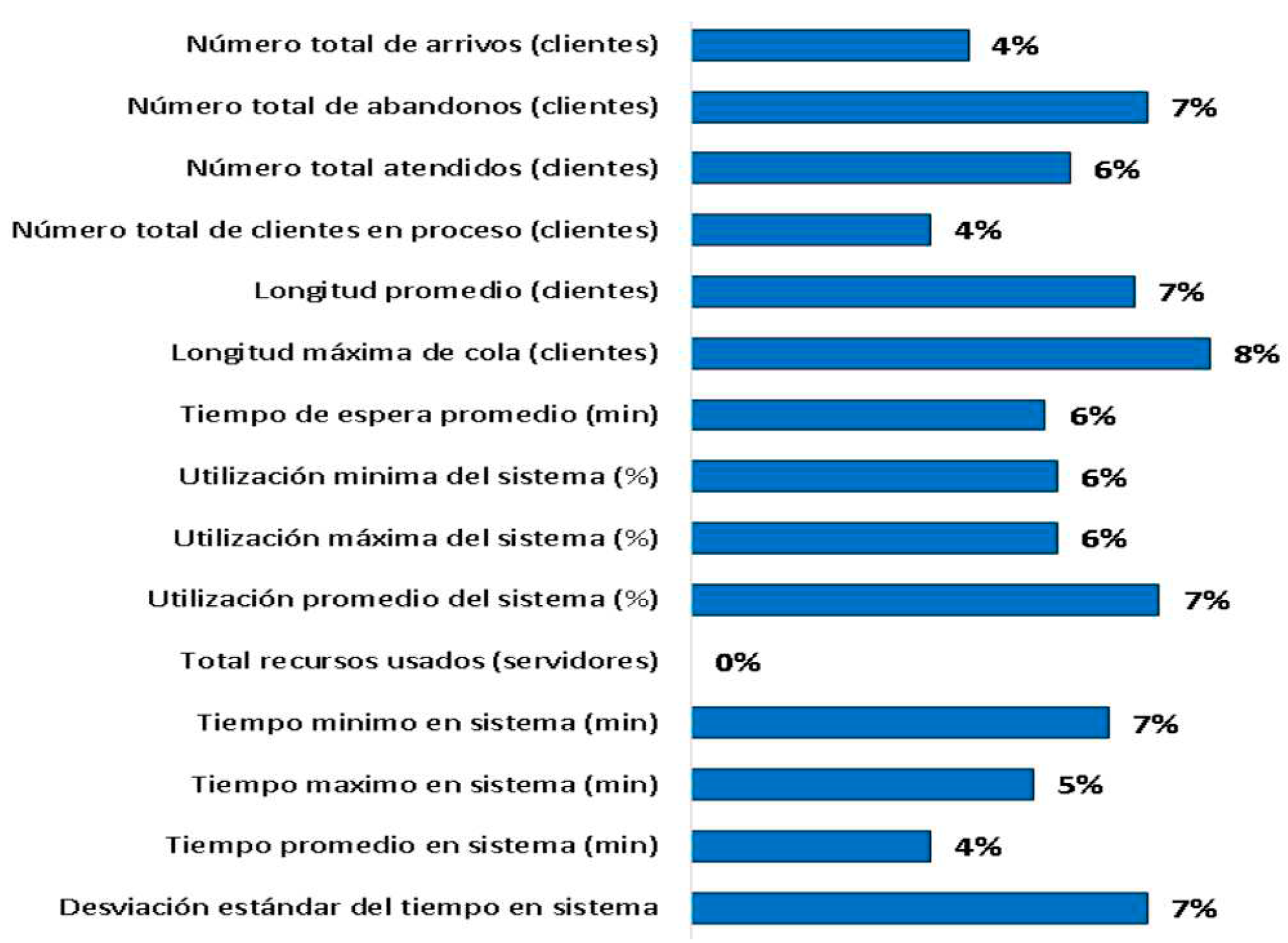
The average error rate in demand (Total number of arrivals), I show an absolute error equal to 4%, that is, the simulated demand is similar to the observed demand. This same reasoning is made for the others, indicators, the maximum queue length, is the one with the highest error rate, reaching 8%, however, it is still valid. The simulated model represents the real system.
3.3. Evaluation of productivity improvement and increase
For the identification of root causes and strategies the Ishikawa diagram or heavy spine was applied (Arango and Angel, 2012).
Figure 10.
Ishikawa diagram.
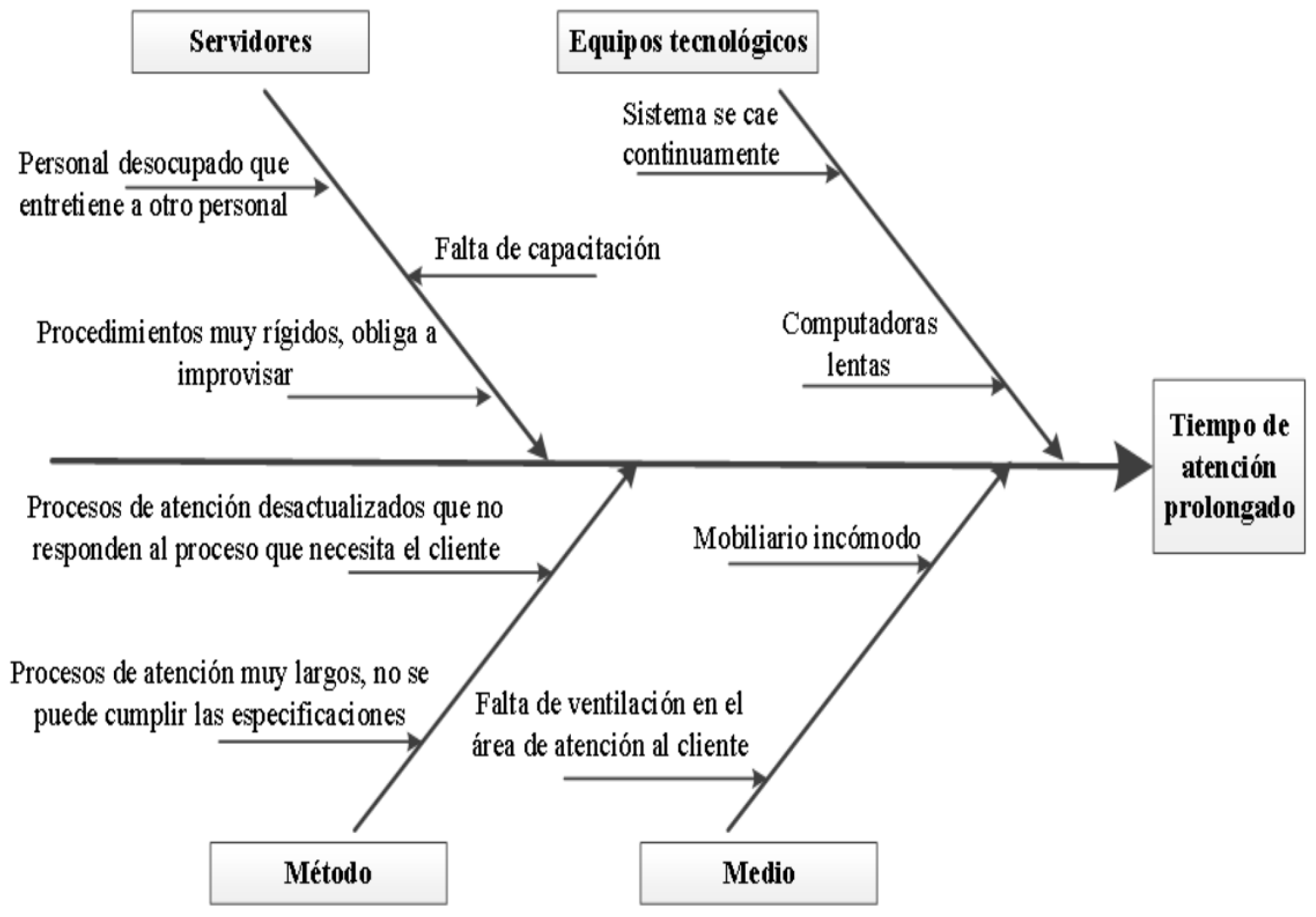
To mitigate the causes that affect attention time, the following strategies were established:
3.3.1. Correction of process instability
By taking into account the capacity indices shown in Table 6 and the control letters, the processes carried out in the customer service center can be characterized as incapable and unstable.
To correct this behavior you must follow these steps:
- Identify hypotheses of the causes of instability, through the involvement of supervisors and servers.
- Analyze the hypotheses obtained from the previous point with the administrative records to confirm the causes of the instability presented in each of the processes.
- Standardize processes through corrections after the evaluation of hypotheses.
- Train servers on new methods and maintain a consistent customer service attitude campaign.
- Perform constant measurements through control letters for the processes to identify if the measures implemented have had a positive effect
The standardization of processes generates a 20% decrease in the variation of the process, with which the results were obtained.
Figure 10.
Variation due to process standardization.
The variation due to the standardization of processes, caused the productivity of the system to increase, before with 17 servers 701 clients were served, with this strategy applied it can be seen that the number of clients served reaches 712. This represents an increase in productivity by 2% of customers served with the same staff.
3.3.2. Setting new specification limits
The company previously established as the specification limits to the time that people remain inside the care center, a maximum time (or upper specification limit, LES) of 15 min and a minimum time of 0 min (lower specification limit, LEI), there is no technical basis with which these limits have been set, That is, the service policy did not consider a technical criterion based on a capacity analysis or a pilot test of the customer service system.
To identify the sensitivity of the capacity indices, a simulation was performed for process A with the increase in the specification limits, which obtained the following results.
Table 8.
Simulated capacity ratings for process A.
| New limits | ||||||
|---|---|---|---|---|---|---|
| 0 a 15,0 | 0,26 | 0,36 | 0,15 | 0,15 | 40,69 | 0,15 |
| 0 a 17,5 | 0,30 | 0,36 | 0,24 | 0,24 | 20,59 | 0,18 |
| 0 a 20,0 | 0,35 | 0,36 | 0,33 | 0,33 | 5,52 | 0,22 |
| 0 a 22,5 | 0,39 | 0,36 | 0,41 | 0,36 | -6,21 | 0,24 |
| 0 a 25,0 | 0,43 | 0,36 | 0,50 | 0,36 | -15,59 | 0,26 |
Although, the objective is not to establish broad specification limits in order to cover the shortcomings of the system, however, establishing new limits will serve to sincerely the value offer without creating false expectations.
3.3.3. Human resource management
When a project is carried out, whatever it may be, one of the indicators that most attention is paid to is the optimization of costs, in the case of the evaluated system, the improvement will be accompanied by the decrease of human resources while continuing to serve customers in an adequate way.
From the simulations carried out, it was observed that, only the elimination of extreme values in the attention times, allowed a notable improvement in the system, the minimum utilization indicator indicates that there is an operator that during the day was occupied 93.04% on Monday and for Friday its use is 39.83%, i.e. its use was reduced by 57%; This revealed the existence of unused capacity.
Table 9.
Impact of human resource management.
| Indicator | Friday (before) | Friday (after) | Variation |
|---|---|---|---|
| Average tail length | 0,11 | 0,36 | 227% |
| Average timeout (min) | 0,07 | 0,39 | 457% |
| Average system utilization (%) | 80,50 | 88,86 | 10% |
| Resources used | 17 | 16 | -6% |
A slight increase in total average utilization was observed, and this change did not affect the queue length, that is, the waiting time was not affected; Except for Mondays, on this day the strategy would be the increase of one person. In one month, a total saving of 959 USD is achieved, in the first year the cost decrease reaches 11 508 USD, therefore, the implementation of this strategy would allow favorable results for the company in terms of increasing the use of the system, reducing costs.
What represented an increase in productivity of 6.28%, with respect to personnel expenses, therefore, the optimization of system expenses was evidenced.
3.3.4. Technical and administrative support
To solve the problems associated with the environment where customer service is carried out and technological tools, this strategy has been developed, which provides specific solutions to each cause:
- System goes down continuously: it is necessary to carry out a review of the means to connect to the internet used by operators, and to propose periodic preventive maintenance
- Slow computers: technical support people should be asked to perform maintenance of computers at both hardware and software level
- Uncomfortable furniture: it would be necessary to repair or replace furniture in poor condition, in addition, provide related implements for the improvement of ergonomics
- Lack of ventilation: A set of simple desktop fans should be incorporated to improve airflow at each workstation
By implementing the improvement strategies together, and considering that the demand does not change and there is an increase in the number of customers served by the implementation of the process standardization strategy, in addition, personnel expenditure decreases due to the improvement in the administration of human resources, the following productivity is obtained:
Table 10.
Increased productivity.
| Strategy | Before | After | Increased productivity |
|---|---|---|---|
| Correcting process instability | 41,23 | 41,88 | 1,57% |
| Human resource management | 0,043 | 0,046 | 6,28% |
| Correction of process instability + Human resource management | 0,043 | 0,046 | 7,76% |
The strategy of establishing new specification limits did not contribute to productivity, this strategy directly affected capacity indexes, however, the administrative support strategy contributed to productivity, however, this must be measured after the implementation of the strategies to be able to quantify what their impact has been.
3.4. Improvement Plan Proposal
In order to establish the guidelines of an improvement and control plan for the care system evaluated, the following stages are detailed below.
Define the project: the problem is that the service center is presenting problems with the attention time of the clients, this caused that people must wait and the total time of permanence of a client within the system can easily exceed an hour. In addition, the value offer offered to the customer of maximum permanence of 15 min is not met, because it causes dissatisfaction in customers.
The project is defined as follows
Name of the project: Improvement of the customer service system.
Project leader: Customer service management.
Description of the problem: Long service times, which causes the client's wait to increase, and therefore, that the total time spent in the service center is extended.
Team members: Head of customer service, head of agency, shift supervisor, servers.
Importance: Customers who remain waiting for a service form an idea of poor quality, in addition to feeling dissatisfied with the treatment they receive.
Objective: To reduce service time and waiting time for customers at the contact center.
Constraints: Human resources cannot be increased due to space limitations, demand cannot be manipulated, the system must adjust to it, and opening hours cannot be extended.
Deliverables: Staff training, monitoring tools and statistical control of processes, improvement of ergonomic conditions of workstations.
Resources: Supervision team, customer service team, administrative requirements (hardware, software, etc.)
Stakeholders: Customers, servers, heads and managers of quality and customer service.
Measure the current situation: for the measurement of the process a set of tools have been established
- Control Letters
- Process capacity indices
- Set of indicators associated with simulations
Analyze to identify the causes: for this section the Ishikawa diagram is used with which the causes of the attention time of the clients were identified.
Implement the solutions: you must implement the identified strategies to mitigate the causes that attention problem in the system.
Control: all the statistical tools used will serve to control the performance of the system.
This improvement plan must be applied until the system meets the specifications and delivers a quality service according to the client's requirements and the new value offer generated by the company.
4. Conclusions
The applied analysis helped in the establishment of a monitoring and control plan for the system studied, in addition, it sets the next starting point for the implementation of the improvements, the average demand is located at 669 people, with a higher demand on Mondays, therefore, they generate a greater queue length reaching 22 people waiting and a general abandonment rate by customers is 5%. The utilization of the system is at 100%, which shows an overload to the system, however, on Fridays the utilization drops to 86%. The average waiting time is 7.67 min. The total time people stay in the system stands at 52.11 min.
The main resource of this system were the servers, and therefore, the efforts must be aimed at providing them: adequate tools, practical methods of customer service, suitable environment and constant training so that the improvements obtained are sustainable over time.
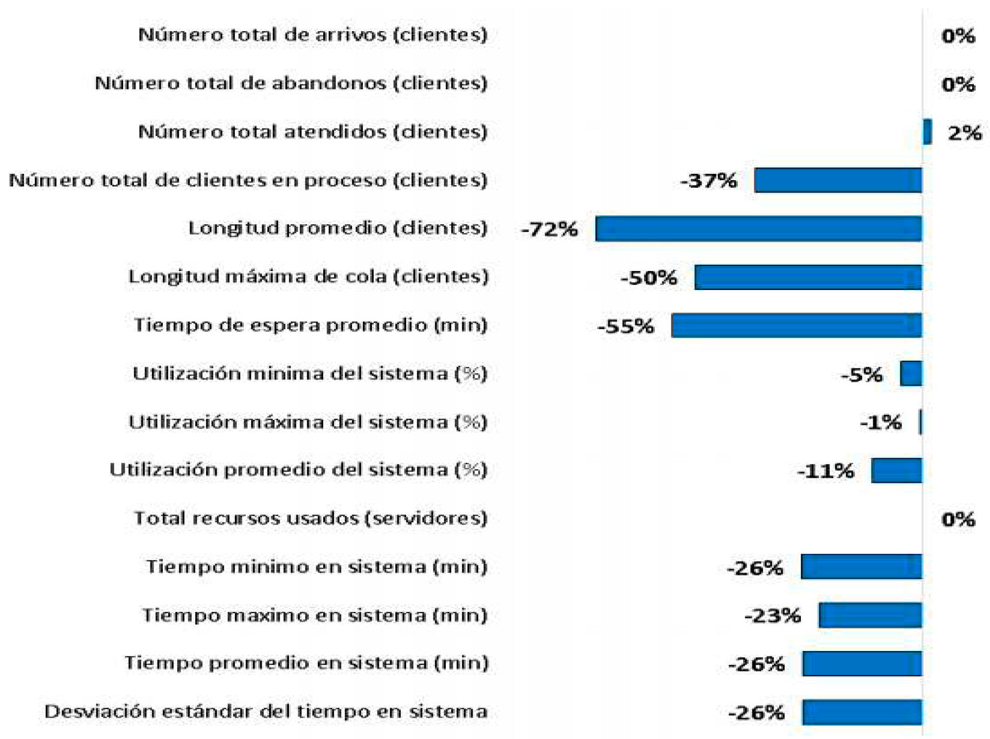
By implementing the improvement strategies, the average waiting time is reduced by 55%, this is also reflected in a reduction in the average length of the queue, which fell by 72%, that is, customers will wait less and queues will be less long as a result of the improvement.
The productivity of customer service with respect to the number of servers increases by 1.57% when standardizing processes, by improving the use of human resources through the management strategy of the same, the productivity of the number of customers served with respect to the expenditure on salaries of the servers grows by 6.28%, By combining the two strategies (serving a greater number of customers and reducing staff), the productivity of the number of customers served with respect to spending on human resource salaries grows by 7.76%. More customers are served at a lower cost.
The service level is located at 20%, at the time of implementing the process standardization strategy, this indicator doubles its performance, and reaches 40%, therefore, the number of customers served under the specification limits goes from 147 to 298 customers.
References
- Arango, D.; Angel, B. Six Sigma Implementation Plan in the admissions process of a higher education institution. Magazine Prospective 2012, 10, 13–21. [Google Scholar] [CrossRef]
- Ariza, F.; Ariza, J. Information and customer service: Certificates of professionalism; McGraw-Hill, 2017. [Google Scholar]
- Chase, R.; Jacobs, R. Operations, Production and Supply Chain Management; McGraw-Hill: Mexico City, Mexico, 2009. [Google Scholar]
- Evans, M.; Morer, X.; Rosenthal, J. Probability and Statistics; Reverté: Barcelona, Spain, 2005. [Google Scholar]
- Gupta, P.; Sri, A. Six Sigma without Statistics: Focus on the search for Immediate Improvements; eBooks2Go, Inc., 2016. [Google Scholar]
- Gutierrez, H. Total Quality and Productivity; McGrawHill: Mexico City, Mexico, 2010. [Google Scholar]
- JaamSim Development Team. The Fastest Simulation Software. 2014. Obtenido de http://jaamsim.com/blog.html (Abril, 2017).
- Montgomery, D.; y Runger, G. Applied Statistics and Probability for Engineers; Wiley: New York, NY, USA, 2003. [Google Scholar]
- Pulido, D. Total Quality Manual for Operators; Limusa, S.A., Ed.; Mexico City, Mexico, 2003. [Google Scholar]
- Ross, S. Simulation; Prentice Hall Hispanoamérica: Mexico City, Mexico, 1999. [Google Scholar]
- Varas, C. Application of DMAIC methodology for the improvement of processes and reduction of losses in the stages of chocolate manufacturing; Universidad de Chile: Santiago de Chile, Chile: 2010. [Google Scholar]
- Bilgen, B.; Şen, M. Project selection through fuzzy analytic hierarchy process and a case study on Six Sigma implementation in an automotive industry. Prod. Plan. Control. 2012, 23, 2–25. [Google Scholar] [CrossRef]
- Butler, M.; Szwejczewski, M.; Sweeney, M. A model of continuous improvement programme management. Prod. Plan. Control. 2018, 29, 386–402. [Google Scholar] [CrossRef]
- Lantz, B.; Rosén, P. Using queueing models to estimate system capacity. Prod. Plan. Control. 2017, 28, 1037–1046. [Google Scholar] [CrossRef]
- Ross, S. M. 8 - Queueing Theory. In Introduction to Probability Models, 12th ed.; Ross, S.M., Ed.; Academic Press: Cambridge, MA, USA, 2019; pp. 507–589. [Google Scholar] [CrossRef]
- Taghizadegan, S. Six Sigma Continuous Improvement. In Essentials of Lean Six Sigma; Taghizadegan, S., Ed.; Elsevier: Amsterdam, The Netherlands, 2006; pp. 43–48. [Google Scholar] [CrossRef]
- Zhang, M.; Wang, W.; Goh, T. N.; He, Z. Comprehensive Six Sigma application: A case study. Prod. Plan. Control. 2015, 26, 219–234. [Google Scholar] [CrossRef]
Table 6.
Capacity indices.
| Process | ||||||
|---|---|---|---|---|---|---|
| A | 0,26 | 0,36 | 0,15 | 0,15 | 40,69 | 0,15 |
| And | 0,26 | 0,39 | 0,13 | 0,13 | 49,28 | 0,14 |
| L | 0,22 | 0,35 | 0,08 | 0,08 | 62,10 | 0,10 |
| In | 0,23 | 0,35 | 0,11 | 0,11 | 51,68 | 0,11 |
Table 7.
Association of causes and mitigation strategies.
| Causes | Strategies |
|---|---|
| Lack of training | Correction of process instability and capacity |
| Rigid procedures | |
| Outdated processes | |
| Very long processes | Set new specification limits |
| Unemployed staff | Human resource management |
| System failures | Technical and administrative support |
| Slow computers | |
| Uncomfortable furniture | |
| Lack of ventilation |
Disclaimer/Publisher’s Note: The statements, opinions and data contained in all publications are solely those of the individual author(s) and contributor(s) and not of MDPI and/or the editor(s). MDPI and/or the editor(s) disclaim responsibility for any injury to people or property resulting from any ideas, methods, instructions or products referred to in the content. |
© 2023 by the authors. Licensee MDPI, Basel, Switzerland. This article is an open access article distributed under the terms and conditions of the Creative Commons Attribution (CC BY) license (https://creativecommons.org/licenses/by/4.0/).
Copyright: This open access article is published under a Creative Commons CC BY 4.0 license, which permit the free download, distribution, and reuse, provided that the author and preprint are cited in any reuse.


