Submitted:
12 July 2023
Posted:
13 July 2023
You are already at the latest version
Abstract
This study addresses the problem of accurately predicting azimuth and elevation angles of signals impinging on an antenna array employing Machine Learning (ML). Using the information obtained at a receiving system when a transmitter’s signal hits it, a Decision Tree (DT) model is trained to estimate azimuth and elevation angles simultaneously. Simulation results demonstrate the robustness of the proposed DT-based method, showcasing its ability to predict the Direction of Arrival (DOA) in diverse conditions beyond the ones present in the training dataset, i.e., the results display the model’s generalization capability. Additionally, the comparative analysis reveals that DT-based DOA estimation outperforms the state-of-the-art MUltiple SIgnal Classification (MUSIC) algorithm, establishing DTs as competitive alternatives for DOA estimation in signal reception systems.
Keywords:
Direction of Arrival
; Machine Learning
; correlation matrix
; Decision Tree
; MUSIC 1. Introduction
1. Introduction
In signal processing, Direction of Arrival (DOA) denotes the direction of signals impinging on a sensor or antenna array [1]. DOA estimation methods have been investigated for decades due to their actual application in radar, sonar, seismology, astronomy, and military surveillance. However, with the development of mobile networks, new technologies, and devices in recent years, DOA has gained new applications and, therefore, more significance. For example, Beamforming (BF) is a technology that is becoming more important every day in mobile communication networks [2]. BF is a technique that focuses a wireless signal toward a specific receiving device rather than having the signal spread in all directions from an omnidirectional antenna, as it usually would. In this way, the received signal level is increased. Then it is essential to know the device’s direction to direct the antenna’s beam toward it previously.
On the other hand, the wide number of drone devices in agriculture, industry, transport, communication, surveillance, etc., along with the development of the Internet of Things (IoT), means that the use of such devices is increasing considerably [3,4]. However, drones can seriously threaten civilian environments or sensitive areas such as airports and military bases. For example, in January 2015, a drone crashed at the White House [5], compromising the security of the government building. On March 29th, 2016, a Lufthansa jet came within 200 feet and collided with a drone near Los Angeles International Airport [6]. On October 12th, 2017, a Beech King Air A100 of Skyjet Aviation collided with an Unmanned Aerial Vehicle (UAV) as the former approached Jean Lesage Airport near Quebec City, Canada. The aircraft landed safely despite being hit on the wing [7].
Due to drones’ security risk facts, as aforementioned, it is necessary to implement drone DOA systems to locate and confiscate or disable them. For the DOA system to work, a drone’s signal is required in order to discover its directions. However, drones’ owners do not want to be discoverable, and they will not transmit such a signal that makes them vulnerable to detection or localization through a DOA system. Fortunately, most drones transmit signals to their controllers to send images, video, and telemetry reports. Another important use case for a DOA system is the localization and recovery of drones that lost contact with their controllers. These drones generally keep sending data to their controllers. Therefore, these signals can be used by DOA systems to find the drone’s direction.
In 5G and 6G wireless networks [8], the estimation of the DOA plays a crucial role across various applications. One of its key benefits lies in facilitating the deployment of smart antenna systems, allowing adaptive steering of antenna arrays to optimize both signal reception and transmission [9]. Moreover, DOA information finds utility in localization and positioning applications, as it enables accurate triangulation of user device locations by estimating the DOA of signals from multiple base stations or access points [10]. Another notable application of DOA estimation pertains to enhancing network security, as the analysis of signal DOAs permits the detection and mitigation of spoofing attacks or unauthorized signal sources [11]. Furthermore, DOA estimation offers valuable insights for network planning and optimization processes, aiding in efficient resource allocation and improved network performance [12].
Hence, due to the importance of the DOA estimation, a new method, based on ML, for finding the azimuth and elevation angles of a signal impinging on a receiving antenna array system is proposed and analyzed in this paper.
2. Related Works
Different studies have been carried out to establish the DOA of an incoming signal [13,14,15,16,17,18,19,20,21,22,23,24,25,26,27,28,29,30,31,32,33,34,35,36,37,38,39,40,41,42]. DOA estimation techniques can be broadly classified into conventional beamforming techniques, Maximum Likelihood Estimator (MLE), and Subspace-Based Techniques (SBT). However, there are recent works on Received Signal Strength (RSS)-based DOA estimation [43]. Moreover, in recent years, ML has been applied to this problem. This section will briefly summarize these techniques and their principal works, which introduce ML to obtain better DOA results.
2.1. Maximum Likelihood Estimation
The MLE finds its estimates by maximizing the probability density function of the observed received signals concerning the model’s parameters. MLE solutions can be classified into two approaches: stochastic MLE and deterministic MLE. In the stochastic MLE, the signals are assumed to be Gaussian distributed [13,14,15]. Deterministic MLE methods consider the signals as being arbitrary and deterministic [15,16]. The sensor noise is modeled as Gaussian in both methods, which is a reasonable assumption due to the central limit theorem. As a result, the stochastic MLE achieves the Cramer-Rao Bound (CRB). On the other hand, this does not hold true for deterministic MLE methods [17].
The problem with MLE techniques is the high computational cost involved since they have to solve a nonlinear multidimensional optimization problem for which global convergence is not guaranteed [18].
2.2. Subspace-Based Techniques
The best-known subspace-based methods are MUSIC [19] and Estimation of Signal Parameters Via Rotational Invariance Techniques (ESPRIT) [20], on which many works have been based. MUSIC-based methods employ the orthogonality of the signal subspace (steering vectors) and the noise subspace to search the spatial spectrum to achieve high resolution. ESPRIT-based methods exploit an underlying rotational invariance among signal subspaces induced by an array of sensors with a translational invariance structure. When the uncertainty of the system or background noise leads to model errors, e.g., the wrong number of sources, subspace-based methods need to solve high-dimensional non-linear parameter estimation problems. Many improved algorithms based on MUSIC and ESPRIT have been developed to estimate the number of sources [21,22]. However, these approaches must sacrifice the array aperture and deteriorate the resolution to deal with the singular matrix of the spatial covariance issue.
2.3. Sparse Signal Reconstruction
The Sparse Signal Reconstruction (SSR) technique has been used in DOA estimation [23,24,25,26,27]. It exploits the property that the spatial spectrum of the point source signals is sparse when the number of signals is limited. The key is to use appropriate non-quadratic regularizing functions (such as -norms), which lead to sparsity constraints and super-resolution. In addition, the primary concern in the SSR technique lies in the computational complexity.
2.4. Machine Learning
ML is presented as a promising technology to be used for DOA estimation. ML-based methods are data-driven and more robust than other methods due to their adaptability to the array geometry and sensor imperfections. They also do not depend on the array geometry shape [44]. In addition, ML offers low-cost implementation and simplicity.
The authors in [28,29,30,31,32,33,34,35,36] used a Neural Network (NN) for DOA estimation. The authors in [28] proposed an azimuth estimation method using a Complex Valued Neural Network (CVNN) for ultra-wideband systems, where the received signal feeds the CVNN. The authors validate their proposal via simulation and experiments. The results are compared to MUSIC and Real-Valued Neural Networks (RVNNs). In [29], it is presented a Multilayer Perceptron Neural Network (MPNN) that can learn from a large amount of simulated noisy and reverberant microphone array inputs for robust DOA estimation. Specifically, the MPNN learns the nonlinear mapping between Generalized Cross-Correlation Vectors (GCC) features and DOA. In [30], the authors used a Deep Neural Network (DNN) for DOA estimation. They evaluated the estimation performance under a scenario where two equal-power and uncorrelated signals are incidents on a Uniform Linear Array (ULA). The authors in [31] focused on scenarios where the number of active sources may exceed the number of simultaneously sampled antenna elements. For this purpose, they proposed new schemes based on NN and estimators that combine NNs with gradient steps on the likelihood function. The authors in [32] propose a cascaded neural network consisting of the SNR classification and the elevation angle estimation for two closely spaced sources. The authors used the correlation matrix as input of a DNN for DOA estimation. In [33], the authors integrate a Multiple Input Multiple Output (MIMO) systems with DNN for channel estimation and to find the DOA of a source. In this work, good results are obtained in the simulations. Still, they only focus on the azimuth angle and require a complex system (e.g., in their simulation, the radio base of the MIMO system is equipped with 128 antennas). In [34], the authors propose a new DOA method based on an ML model to estimate the azimuth angle of a signal. A dataset named “Dround Data New” was obtained with a four antennas-based system that contains well-known received powers. The authors trained and validated the dataset with a DNN model. In [35], the authors presented a deep ensemble learning to find a source’s azimuth and elevation angles to different training conditions. The authors designed a Convolutional Neural Network (CNN) that performs the regression task to learn a mapping between the spatial covariance matrix of the received signals from the antenna elements and the DOA. In addition, to improve the prediction performance, they proposed an ensemble learning method. Simulation results show that their proposals have slightly lower Mean Squared Error (MSE) performance than conventional methods such as MUSIC and -SVD (Singular Value Decomposition). However, the simulation results also show that the authors’ proposals in this article respond very fast and have higher speeds than the MUSIC and -SVD algorithms. In [36], the authors proposed Circularly Fully Convolutional Networks (CFCN) to find the DOA of multiple sources in low-frequency scenarios. The CFCN is trained by the data set labeled by space-frequency pseudo-spectra and provided on-grid DOA proposals. Then, the regression model is developed to estimate the precise DOAs according to corresponding proposals and features.
In [37,38,39,40,41,42], the authors proposed a Support Vector Regression (SVR)-based DOA estimation method. In [37], a smart antenna system is considered to estimate the DOAs of multiple sources in noiseless and noisy environments. In [38], the problem of estimating the DOAs of coherent electromagnetic waves impinging upon a ULA is considered an extension of previous work collecting experimental results. In [39], a multi-resolution approach for the real-time DOA estimation of multiple signals impinging on a planar array is presented. The method is based on a Support Vector Classifier (SVC), and it exploits a multi-scaling procedure to enhance the angular resolution of the detection process in the regions of incidence of the incoming waves. The authors in [40] proposed the combination of the advantages of Forward–Backward Linear Prediction (FBLP) and SVR in estimating DOAs of coherent incoming signals with low snapshots. In [41], the authors proposed a scheme to address the wideband DOA estimation problem. An approach for the real-time DOA estimation of multiple signals impinging on a planar array is presented in [42]. This last work estimates the azimuth and elevation angles of one or more incident sources in a ULA. However, the angular resolution is shallow. The main disadvantage of Support Vector Machine (SVM) is the algorithm’s time complexity [45]. The algorithmic complexity of SVM models affects the model training time on large datasets, the development of optimal models for multiclass, and the performance on unbalanced datasets.
Table 1 summarizes the articles mentioned above that employ ML techniques to solve the DOA problem. The table shows the main aspects considered to carry out our work. In addition, the table collects the angles the related works consider: azimuth, elevation, or both. It also shows if the work is oriented to find the DOA from a single source or several, if the proposals were validated via simulation or experiments, and if the results were compared with an existing DOA model.
ML has been mainly used to improve the estimation of azimuth or elevation angles and computing speed. In addition, various studies have been carried out to find the origin of multiple sources. However, the study of ML-based DOA for estimating azimuth and elevation angles has yet to be deeply studied. The reason behind this is the huge size of the training data, which is only supported by some models like NNs [46]. However, estimating the elevation and the azimuth angles is crucial and has many applications in various engineering fields. For instance, with complete DOA information, it is possible to improve the transmission coverage in wireless communications by avoiding interference and enhancing the system capacity [42]. More specifically, the knowledge of the azimuth and elevation angles would bring better exploitation of the BF technology in the Next-Generation of mobile networks. Therefore, this study addresses the problem of accurately predicting the azimuth and elevation angles of a signal impinging on an antenna array.
The main goal of this work is to propose a simple, in terms of computational complexity, yet accurate ML model for DOA estimation that predicts both the azimuth and elevation angles. To achieve this goal, the following specific objectives are considered:
- Design a receiving antenna system to estimate the DOA.
- Propose an ML-based DOA estimation solution capable of adapting to different conditions, such as the SNR of the signal.
- Discuss training data preparation and design for a specific scenario.
- Optimize the ML-based DOA estimation solution.
- Compare the results obtained with the ML-based DOA estimation solution with a state-of-the-art DOA estimation method present in the literature.
3. System model
We consider a receiving system that consists of a single-channel receiver and M half-wavelength strip dipole antennas operating at a frequency of 70 MHz 1 [47,48]. Therefore, only one antenna is connected to the receiver at a time. The M antennas are uniformly placed along a circle of radius, , forming a Uniform Circular Array (UCA) as shown in Figure 1, where is the incident signal’s wavelength.
If a signal impinges on the center of the circle formed by the M antennas with azimuth, , and elevation, , angles as shown in Figure 1, the received signal at the m-th antenna element can be mathematically given as
where is the antenna index, is the sample index, (, , ) represents the attenuation factor (amplitude attenuation and phase shift) of the m-th antenna, s(k) is the k-th signal transmitted by the source as it arrives at the antenna array and (k) is the k-th noise sample at the m-th antenna, which has its value drawn from a circularly-symmetric (central) complex normal distribution with variance equal to . The attenuation factor, (, , ), is expressed as
where r is the radius of the receiving system, and is the angular position of the antenna array elements, which can be calculated as
Therefore, the received signal vector obtained at the output of the antenna array can be written as
which can be re-expressed as
where denotes the transpose and A, s(k), and n(k) are given by
and
with dimensions , , and , respectively.
The spatial correlation matrix of the array output is usually used for DOA estimation since it contains sufficient information about the received signals. From (5), the spatial correlation matrix, R, of the received noisy signals can be expressed as
where is the statistical expectation operator, the superscript H denotes the complex conjugate transpose operation and is the element in the i-th row and j-th column.
After applying the expectation operator, (9) can be rewritten as
where represents the noise power (i.e., the variance) at the array elements, I is the identity matrix with dimensions M×M, and is the K×K signal correlation matrix that is written as
Now the problem boils down to finding the angle of azimuth and elevation between the center of the receiving system and the source (i.e., , , respectively), having as input data the correlation matrix, R, of the receiving system. The correlation matrix can be unbiasedly estimated through the sample correlation matrix
where N is the number of independent observations considered for calculating the matrix.
4. Proposed method
Figure 2 summarizes our proposal to find the azimuth and elevation angles of a source signal impinging on a receiver system. The proposed method will be divided into the ML model’s setup process (Process 1 - blue colored boxes) and the up-and-running process (Process 2 - yellow colored boxes). First, both processes are fed with the output of the antenna array in response to the source signal impinging on it. Next, the steps involved in these two processes are described.
Step 1 - Data collection: This work uses supervised learning to find and angles. In supervised learning, the training data fed to the ML algorithm includes pairs of fixed-dimension feature vectors and the desired output, called labels. In this step, the received signal obtained at the output of the antenna array Y and their respective labels are collected (azimuth and elevation angles that the transmitter forms with the center of the array). Y is the matrix formed by the K received signal vectors obtained at the output of the antenna array
where K is the number of collected vector samples.
In this work, we assume the size of the dataset is L. In that case, the fixed-dimensional feature vectors are composed of L spatial correlation matrices, , which are converted into vectors, and the labels are their respective azimuth and elevation angles formed between the transmitter and the center of the receiving system (i.e., , , …, and , , …, ), where , , …, are values between 0 and 2 radians and , , …, are values between 0 and /2 radians.
Step 2 - Data preprocessing: The preprocessing of the data is essential to achieve good performance with the ML algorithms. At this point, the L correlation matrices are calculated from the samples of the signals received by the receiving system, and their redundant information is removed. Since the correlation matrices are conjugate-symmetrical concerning their diagonal, the elements of their upper or lower triangular part provide enough information for 2D DOA estimation. This way, the other part of the matrix can be ignored. Therefore, next, we create feature vectors with the upper triangular part of the L correlation matrices, , (which includes the main diagonal) with dimensions equal to .
In addition, the matrices contain complex values that can not be interpreted by most ML models, so they will be separated into real and imaginary parts and arranged in a vector as follows
with dimension and where and are the real and imaginary parts of the element in the i-th row and j-th column of l-th correlation matrix, respectively.
Step 3 - Data splitting: To validate the ML models, it is necessary to take part of the input data for training and another part, known as a validation set, usually smaller than the previous one, to evaluate the model when presented with unseen data, i.e., measure its generalization capacity. The validation set is used to evaluate the different metrics for the ML model by comparing the model’s predicted label with the actual value in the set. This way, it is possible to assess whether the model learned a general solution or not.
Step 4 - Building/Training the ML model: In this step, the ML model is set up by choosing various strategies to improve the training results. First, we can select various ML regression models, for example, DT, Random Forest (RF), SVC, NN, etc. Specifically, in this work, we will work with the DT model. This model was chosen based on results obtained and published in [49]. DT models are one of the simplest yet most successful and powerful forms of ML models [50]. This work uses the sklearn.tree.DecisionTreeRegressor [51] class from the Scikit-Learn (sklearn) library [52]. This class allows Multi-Output Multi-Labels, which gives us the advantage that several variables, such as the azimuth and elevation angles, can be found simultaneously with a single model.
Then, we can apply optimization tools to the selected model to improve its prediction results considerably. Automated Hyperparameter Optimization (HPO) reduces the human effort necessary for optimizing ML models, improves algorithms’ performance, and improves scientific studies’ reproducibility and fairness. There are different open-source software such as sklearn.model_selection.GridSearchCV [53], Talos [54], and Optuna [55] that facilitate the automation of hyperparameter optimization. In this work, we will employ Optuna for being simple, well-known, and producing excellent results.
Optuna’s optimization algorithm is divided into sampling and pruning strategies, each playing a distinct role. The sampling strategy leverages Bayesian optimization [56], utilizing the historical data to determine the next set of hyperparameters or configurations. On the other hand, the pruning strategy enables faster optimization by identifying and discarding unpromising trials based on learning curves. Optuna offers numerous advantages that greatly influenced our decision to choose this tool. The key highlights of these advantages are outlined next.
- Lightweight, versatile, and platform-agnostic architecture that can be effortlessly integrated into various environments, allowing for easy adoption and usage.
- Handling a wide variety of hyperparameter optimization tasks that offers flexibility and robustness to tackle various optimization scenarios effectively.
- Pythonic way of coding using familiar Python syntaxes that simplifies the process of defining and exploring complex search spaces, enhancing user convenience and code readability.
- Efficient optimization algorithms, including state-of-the-art techniques for sampling hyperparameters and pruning unpromising trials, that lead to improved optimization performance and faster convergence toward optimal solutions.
- Easy parallelization that allows the scaling of studies to tens or hundreds of workers with minimal or no code modifications, accelerating the optimization process, particularly when dealing with computationally intensive tasks.
- Quick visualization capabilities that enable swift inspection and analysis of optimization histories. It provides a range of plotting functions that allow for easy interpretation and understanding of the optimization process.
Step 5 - Validating the ML model: After training the ML model, we validate it using part of the pre-processed data intended for this purpose (i.e., the validation dataset), that is, the part that was not used to train the ML model. For this, a prediction of the labels corresponding to the feature vectors of the validation set is made and compared with the actual labels. From here, we can obtain satisfactory or unsatisfactory results depending on whether the predicted labels are more or less similar to the actual ones. We analyze the results and adjust the ML model accordingly if the results are unsatisfactory.
There are different metrics to analyze how satisfactory the results of the ML model were. In this work, we will use the Root-Mean-Square Error (RMSE). The RMSE of an estimator measures the square root of the average of the squares of the errors, that is, the square root of the average of the squared difference between the estimated and the actual values. The RMSE for the proposed Multi-Output Multi-Label Proposal (MMP) is calculated as follows
where , are the actual azimuth and elevation angles and , are the azimuth and elevation angles predicted by the ML model, respectively.
Step 6 - Data preprocessing: The same pre-processing as the one described in Step 2 is carried out for new data samples collected during the operational use of the proposed DOA estimation method.
Step 7 - Operational step: Once satisfactory results are obtained, the trained and optimized ML model can be used to predict the azimuth and elevation angles of new data samples.
5. Experimental Results
In this section, we describe how the dataset was generated and present several experimental results used for assessing the proposed DOA estimation method. In the first part, we discuss how the dataset was created. Next, we analyze the robustness of the method. Finally, in the third part, we compare it with a well-known DOA estimation algorithm.
All receiving models are simulated in Matlab, and the collected information is used to create the dataset. The Python language and the Scikit-Learn library are used to implement the DT-based DOA estimation method. All experiments are performed on an Acer laptop with a Core i7 processor, 16 GB of RAM memory, and an 8 GB Intel(R) Iris(R) Xe graphics video card.
5.1. Data Generation
Based on the system model described in Section 3 and using the Matlab simulation tool, we generated the dataset that was used for training and validating the proposed DT-based DOA estimation method. Matlab was also used to generate the radiation patterns of the half-wavelength strip dipole antennas.
For each pair of azimuth and elevation angles, i.e., (, ), the corresponding l-th correlation vector, , was obtained. The azimuth and elevation angles are in the range [0, 360) and [0, 90), respectively, with an angular resolution of 1. For each angle pair, 20 correlation vectors, , were generated. Each correlation vector corresponds to a realization of the AWGN channel. This way, the total number of correlation vectors, , generated is equal to 648.000, i.e., 20 noise realizations × 360 azimuth angles × 90 elevation angles. It is assumed that , ∀k, and is circularly symmetric, independent, and identically distributed complex AWGN with zero mean and variance in the range to 10. Moreover, we are going to compare the proposed method for a different number of receiving antennas, 4, 8, and 12.
5.2. Analysis of the robustness of the ML model
In this section, we assess the robustness of the ML model against variations in the received signal. Let’s suppose all data in the collected database have the same noise variance. In that case, there is a significant probability that when the received signal has a different noise variance, the model will predict the wrong angles because it was trained with a dataset generated with signals having a different noise variance. For example, if the DT model is trained with correlation vectors of signals with an SNR of dB, the model could incorrectly predict the azimuth and elevation angles when the received signal has an SNR of 20 dB.
To analyze if the DT model can correctly predict the DOA angles when it is trained with a signal with an SNR value different from the SNR of the signal for which the DOA is to be predicted, we will carry out two experiments described next.
- Experiment 1: For a given number of receiving antennas, M, one single DT model is trained with a dataset comprising correlation vectors of signals of all SNR values in the set -10, 0, 10, 20, 30, and 40 dB. Subsequently, also for a specific number of receiving antennas, the model is validated with datasets composed of correlation vectors of each individual SNR value. This training and validation process is repeated for each different number of receiving antennas considered ( 4, 8, and 12).
- Experiment 2: For a given number of receiving antennas, M, different DT models are trained with a dataset containing correlation vectors of one specific SNR value in the set -10, 0, 10, 20, 30, and 40 dB. Subsequently, also for a specific number of receiving antennas, the models are validated with datasets composed of correlation vectors of each individual SNR value. This training and validation process is repeated for each different number of receiving antennas considered ( 4, 8, and 12).
5.2.1. Experiment 1 - Results
To perform this experiment, 19 examples of each combination of angles and SNR values were used for training purposes. The azimuth angles are between 0 and 359, and the elevation angles range from 0 to 89 with a resolution of 1. One DT model was trained with a dataset composed of correlation vectors with SNR values of -10, 0, 10, 20, 30, and 40 dB. In other words, 3.693.600 (i.e., 19 × 360 × 90 × 6) samples (i.e., correlation vectors) were used for training the DT model. On the other hand, one example of each combination of angles and SNR value was used to validate the model for each SNR value, generating 6 datasets with 32.400 (i.e., 1 × 360 × 90) samples each. Optuna was employed to optimize the hyperparameters of the DT model. This process (i.e., training, optimization, and validation) is repeated for each number of receiving antennas in the set 4, 8, and 12. The obtained hyperparameter optimization results for all antenna numbers are presented in Table 2.
Figure 3 shows the RMSE versus SNR values attained by the DT models trained with correlation vectors containing all SNR values and for different numbers of receiving antennas. The models were validated with 6 datasets, each one comprising correlation vectors with a unique SNR value. Figure 3a) shows the RMSE of the DT models when simultaneously predicting the azimuth and elevation angles. Figure 3b,c) show the RMSE of the DT models when predicting the azimuth and elevation angles, respectively.
Figure 3 as a whole shows that the DT model’s estimation performance improves as the number of antennas increases. It is expected since the available correlation information increases. Moreover, the figure also shows that training the DT model with a dataset comprised of correlation vectors with different SNRs presents good performance.
Figure 4 shows the SNR versus the actual and predicted angles for (Figure 4 a, b, and c) and (Figure 4 d, e, and f), respectively. As the number of antennas of the receiving system increases, the diagonal becomes narrower (i.e., less noisy), both in the prediction of and angles, which means a greater correspondence between the actual and predicted angles. Furthermore, for the same number of receiving system antennas, the sharpness of the diagonal improves as the SNR increases.
In addition, when looking at Figure 4 and comparing the predictions of and angles, one might be made to believe that the model better predicts the angle, which is contradicted by the results in Figure 3 b and c. This happens because angles are in a shorter interval, [0, 90), than angles, [0, 360). As a matter of fact, in order to plot the results shown in Figure 4, the DT model performs the same number of predictions for and angles. This means that the DT model has more information to learn from in order to estimate the elevation angle compared to the azimuth angle, making it easier for the model to estimate elevation angles than the azimuth ones. Therefore, when plotting the same number of points (i.e., predictions) in a smaller space, the points seem more dispersed, and consequently, the diagonal seems less narrow (i.e., is less defined) when compared with the diagonal of the azimuth angles.
5.2.2. Experiment 2 - Results
To perform this experiment, 19 examples of each combination of angles and one specific SNR value were used to train one model. In total, 615.600 (19 × 360 × 90) samples of one given SNR value were used to train the DT models. An example of each combination of angles and specific SNR was used to validate the models.
As in Experiment 1, we first use Optuna to optimize the hyperparameters of the models. Since we want to train DT models for different numbers of antennas and specific SNR values, we are going to have a total of 18 models (i.e., models for 4, 8, and 12 antennas that are trained with datasets composed of 6 different SNR values, -10, 0, 10, 20, 30, and 40 dB). The obtained hyperparameter optimization results for all SNR values and antenna numbers are presented in Table 3.
Figure 5 shows the results of training the DT models with correlation vectors of the received signals. Each model was trained with a dataset composed of correlation vectors of signals with one specific SNR and then validated with correlation vectors of signals with different SNRs. The x-axis shows the SNR of the signals with which the DT model was trained, and the y-axis shows the average RMSE of validating the DT models with signals with SNRs of -10, 0, 10, 20, 30, and 40 dB. When analyzing the results shown in Figure 5, it is observed that, globally, particularly for , the DT models exhibit improved capabilities in predicting azimuth and elevation angles of signals with varying SNRs when trained with signals possessing an SNR of approximately 20 dB. Therefore, next, we use models trained with signals having an SNR of approximately 20 dB.
Figure 6 displays the validation results of DT models trained with correlation vectors presenting an SNR of 20 dB. The validation is performed using correlation vectors presenting SNR values ranging from -10 dB to 40 dB (x-axis). The graph illustrates that training the DT model with correlation vectors of signals at an SNR of 20 dB and validating it with SNR signals from -10 dB to 40 dB yields satisfactory performance. Moreover, Figure 7 demonstrates consistent predictions of azimuth and elevation angles when training the model with signals at an SNR of 20 dB. Once more, we see that the diagonal becomes narrower as the number of antennas and SNR increase.
5.2.3. Comparison between experiments 1 and 2
Let’s delve into the comparison of the results obtained from experiments 1 and 2 (i.e., Figure 3 and Figure 6, respectively). Upon careful analysis, it becomes apparent that the results of experiment 1 outshine those achieved in experiment 2. Notably, experiment 1 showcases a smaller RMSE for both low SNR values and a limited number of antennas, as small as 4. This compellingly signifies that training a DT model with a diverse dataset containing correlation vectors encompassing various SNR values proves to be a superior approach compared to training the model with signals having a specific SNR value.
These results highlight the efficacy of employing DT models in accurately estimating azimuth and elevation angles across a wide range of SNR values. While experiment 1 outperformed experiment 2 in terms of RMSE, both experiments demonstrate the overall efficiency and robustness of proposals utilizing DT models in handling a broad range of SNR values. This reaffirms the potential of DT-based methodologies for accurate angle estimation, providing valuable insights into their application in real-world scenarios.
5.3. Comparison with MUSIC
Finally, let’s compare the results of the well-known MUSIC DOA estimation algorithm with our proposed method [19]. In this work, we use the Matlab implementation of the algorithm [57]. In Figure 8 a), we observe the MUSIC results for the resolution of the same azimuth and elevation angles as resolved by the DT model. Comparing the results of MUSIC with those of Experiments 1 and 2 (Figure 8 b) and c), respectively), it becomes apparent that, on the whole, the DT model achieves superior performance.
MUSIC demonstrates superior efficiency than the DT model for both experiments only when M is equal to 4 antennas. However, for experiment 1, , and signals with SNR values greater than 0 dB, the DT model exhibits greater accuracy. For this case, as the number of antennas increases, the DT model continuously improves its accuracy, whereas the accuracy of MUSIC remains relatively constant for SNR values greater than 0 dB and M equal to 8 and 12 antennas. For M equal to 4 antennas, MUSIC only shows a constant performance for SNR values greater than 20 dB. As for experiment 2, it is clearly noticeable that the DT model only outperforms MUSIC for SNR values greater than 10 dB and . When comparing the two experiments, it is straightforwardly visible that experiment 1 outdoes experiment 2. All in all, these results clearly demonstrate that the proposed DT-based method successfully estimates DOA across an SNR range with satisfactory RMSE.
The comparison between the DT model and the MUSIC algorithm underscores the advantages of our approach in achieving accurate DOA estimation. The DT model outperforms MUSIC in terms of accuracy, especially for signals with higher SNR values. Additionally, the DT model showcases the ability to leverage an increasing number of antennas to enhance accuracy, which is not observed in the case of MUSIC.
Next, let’s examine Figure 9 a), which displays the average time taken by the MUSIC algorithm to estimate the azimuth and elevation angles. Additionally, Figure 9 b) and c) illustrate the average time consumed by the DT models in Experiments 1 and 2, respectively. Upon comparing these figures, it becomes apparent that, in general, the average prediction times of DT models are shorter than the average prediction time of the MUSIC algorithm.
This finding not only reinforces the superior accuracy demonstrated by DT models, as discussed earlier in terms of RMSE results but also highlights their efficiency in terms of prediction time. The reduced prediction times indicate that DT models offer a faster computational approach to achieving accurate DOA estimation when compared to the conventional MUSIC method.
By excelling in both accuracy and computational efficiency, our model exhibits a clear advantage over the MUSIC algorithm. These results validate the effectiveness of the DT models, providing a solid foundation for their practical implementation in real-world scenarios where timely and precise DOA estimation is of utmost importance.
6. Conclusions
In conclusion, DOA estimation has been a widely researched topic in signal processing, with applications spanning various fields such as beamforming, localization in 5G and 6G networks, drone localization, radar, sonar, seismology, astronomy, and military surveillance, among others.
Therefore, by recognizing the significance of DOA estimation, this study has proposed and analyzed a novel method based on DTs for accurately determining the azimuth and elevation angles of signals impinging on a receiving antenna array system. The primary objective of this proposed method is to improve the accuracy, efficiency, and applicability of DOA estimation.
The DT models employed in this method are capable of estimating the azimuth and elevation angles between a transmitter and a system receiver. They utilize information provided by the correlation matrix derived from the signals received by an antenna system. To enhance the training and prediction processes of the DT models, their hyperparameters have been optimized using the Optuna framework.
Two experiments were conducted to demonstrate the effectiveness of the proposed solution in predicting the azimuth and elevation angles under different conditions from those used during the training of the ML model. The results from both experiments indicate that the DT models employed in the proposed method can effectively learn to predict azimuth and elevation angles with signals characterized by varying SNRs. When compared to the MUSIC DOA estimation algorithm, the proposed solution exhibited significantly better results in minimizing both the RMSE and the average prediction time.
In future research, it would be valuable to explore and evaluate the performance of alternative types of receiving systems and ML models, including neural networks. Furthermore, the proposal presented in this study, as well as future ones, should be validated through real-world experiments to complement the findings obtained from simulations. Such real experiments would provide further validation and ensure the practical viability of the proposed solutions.
Author Contributions
Conceptualization A.R.C., J.M.C.B., and F.A.P.d.F.; investigation A.R.C.; writing—original draft preparation A.R.C.; writing—review and editing A.R.C., J.M.C.B., and F.A.P.d.F.; supervision J.M.C.B., and F.A.P.d.F.; project administration J.M.C.B. All authors have read and agreed to the published version of the manuscript.
Funding
This work was partially supported by the Coordenação de Aperfeiçoamento de Pessoal de Nível Superior - Brazil (CAPES) and RNP, with resources from MCTIC, Grant Nos. 01250.075413/2018-04 and 01245.010604/2020-14, under the 6G Mobile Communications Systems of the Radiocommunication Reference Center (Centro de Referência em Radiocomunicações - CRR) project of the National Institute of Telecommunications (INATEL), Brazil; by Huawei, under the project Advanced Academic Education in Telecommunications Networks and Systems, Grant No. PPA6001BRA23032110257684; by Fundação de Amparo à Pesquisa do Estado de Minas Gerais (FAPEMIG) via grant number 2070.01.0004709/2021-28; by FCT/MCTES through national funds and when applicable co-funded EU funds under the Project UIDB/EEA/50008/2020; and by the Brazilian National Council for Research and Development (CNPq) via Grant Numbers 313036/2020-9 and 403827/2021-3; and the MCTI/CGI.br and the São Paulo Research Foundation (FAPESP) under Grant No. 2021/06946-0.
Abbreviations
| ML | Machine Learning |
| DT | Decision Tree |
| DOA | Direction of Arrival |
| BF | Beamforming |
| IoT | Internet of Things |
| UAV | Unmanned Aerial Vehicle |
| MLE | Maximum Likelihood Estimator |
| SBT | Subspace-Based Techniques |
| RSS | Received Signal Strength |
| CRB | Cramer-Rao Bound |
| MUSIC | Multiple Signal Classification |
| ESPRIT | Estimation of Signal Parameters Via Rotational Invariance Techniques |
| SSR | Sparse Signal Reconstruction |
| NN | Neural Network |
| CVNN | Complex Valued Neural Network |
| RVNN | Real-Valued Neural Network |
| MPNN | Multilayer Perceptron Neural Network |
| GCC | Generalized Cross-Correlation Vectors |
| DNN | Deep Neural Network |
| ULA | Uniform Linear Array |
| MIMO | Multiple Input Multiple Output |
| CNN | Convolutional Neural Network |
| MSE | Mean Squared Error |
| SVD | Singular Value Decomposition |
| CFCN | Circularly Fully Convolutional Networks |
| SVR | Support Vector Regression |
| FBLP | Forward–Backward Linear Prediction |
| SVM | Support Vector Machine |
| AWGN | Additive White Gaussian Noise |
| HPO | Automated Hyperparameter Optimization |
| RMSE | Root-Mean-Square Error |
| MMP | Multi-Output Multi-Label Proposal |
| UCA | Uniform Circular Array |
| SNR | Signal-to-Noise Ratio |
References
- Chen, Z.; Gokeda, G.; Yu, Y. Introduction to Direction-of-arrival Estimation; Artech House, 2010. [Google Scholar]
- Brilhante, D.d.S.; Manjarres, J.C.; Moreira, R.; de Oliveira Veiga, L.; de Rezende, J.F.; Müller, F.; Klautau, A.; Leonel Mendes, L.; de Figueiredo, F.A.P. A Literature Survey on AI-Aided Beamforming and Beam Management for 5G and 6G Systems. Sensors 2023, 23. [Google Scholar] [CrossRef] [PubMed]
- Lahoti, S.; Lahoti, A.; Saito, O. Application of unmanned aerial vehicle (UAV) for urban green space mapping in urbanizing Indian cities. Unmanned Aerial Vehicle: Applications in Agriculture and Environment 2020, 177–188. [Google Scholar]
- Allahham, M.S.; Khattab, T.; Mohamed, A. Deep learning for RF-based drone detection and identification: A multi-channel 1-D convolutional neural networks approach. 2020 IEEE International Conference on Informatics, IoT, and Enabling Technologies (ICIoT); IEEE, 2020; pp. 112–117. [Google Scholar]
- Drone That Crashed at White House Was Quadcopter. Available online: https://time.com/3682307/white-house-drone-crash/ (accessed on 20 March 2023).
- Lufthansa jet and drone nearly collide near LAX. Available online: https://www.latimes.com/local/lanow/la-me-ln-drone-near-miss-lax-20160318-story.html/ (accessed on 20 March 2023).
- Aviation Investigation Report A17Q0162. Available online: https://www.tsb.gc.ca/eng/rapports-reports/aviation/2017/a17q0162/a17q0162.html/ (accessed on 20 March 2023).
- Dala Pegorara Souto, V.; Dester, P.S.; Soares Pereira Facina, M.; Gomes Silva, D.; de Figueiredo, F.A.P.; Rodrigues de Lima Tejerina, G.; Silveira Santos Filho, J.C.; Silveira Ferreira, J.; Mendes, L.L.; Souza, R.D.; Cardieri, P. Emerging MIMO Technologies for 6G Networks. Sensors 2023, 23. [Google Scholar] [CrossRef]
- Dhope, T.; Simunic, D.; Djurek, M. Application of DOA estimation algorithms in smart antenna systems. Studies in informatics and Control 2010, 19, 445–452. [Google Scholar]
- Zhang, Y.; Wang, D.; Cui, W.; You, J.; Li, H.; Liu, F. DOA-based localization method with multiple screening K-means clustering for multiple sources. Wireless Communications and Mobile Computing 2019, 2019, 1–7. [Google Scholar] [CrossRef]
- Meurer, M.; Konovaltsev, A.; Appel, M.; Cuntz, M. Direction-of-arrival assisted sequential spoofing detection and mitigation 2016.
- Zhou, Z.; Liu, L.; Zhang, J. FD-MIMO via pilot-data superposition: Tensor-based DOA estimation and system performance. IEEE Journal of Selected Topics in Signal Processing 2019, 13, 931–946. [Google Scholar] [CrossRef]
- Paik, J.W.; Lee, K.H.; Lee, J.H. Asymptotic performance analysis of maximum likelihood algorithm for direction-of-arrival estimation: Explicit expression of estimation error and mean square error. Applied Sciences 2020, 10, 2415. [Google Scholar] [CrossRef]
- Pesavento, M.; Gershman, A.B. Maximum-likelihood direction-of-arrival estimation in the presence of unknown nonuniform noise. IEEE Transactions on Signal Processing 2001, 49, 1310–1324. [Google Scholar] [CrossRef]
- Athley, F. Threshold region performance of maximum likelihood direction of arrival estimators. IEEE Transactions on Signal Processing 2005, 53, 1359–1373. [Google Scholar] [CrossRef]
- Dong, Y.Y.; Dong, C.X.; Liu, W.; Liu, M.M. DOA estimation with known waveforms in the presence of unknown time delays and Doppler shifts. Signal Processing 2020, 166, 107232. [Google Scholar] [CrossRef]
- Stoica, P.; Nehorai, A. MUSIC, maximum likelihood, and Cramer-Rao bound. IEEE Transactions on Acoustics, speech, and signal processing 1989, 37, 720–741. [Google Scholar] [CrossRef]
- Stoica, P.; Sharman, K.C. Maximum likelihood methods for direction-of-arrival estimation. IEEE Transactions on Acoustics, Speech, and Signal Processing 1990, 38, 1132–1143. [Google Scholar] [CrossRef]
- Schmidt, R. Multiple emitter location and signal parameter estimation. IEEE transactions on antennas and propagation 1986, 34, 276–280. [Google Scholar] [CrossRef]
- Roy, R.; Kailath, T. ESPRIT-estimation of signal parameters via rotational invariance techniques. IEEE Transactions on acoustics, speech, and signal processing 1989, 37, 984–995. [Google Scholar] [CrossRef]
- Zhou, L.; Zhao, Y.j.; Cui, H. High resolution wideband DOA estimation based on modified MUSIC algorithm. 2008 International Conference on Information and Automation; IEEE, 2008; pp. 20–22. [Google Scholar]
- Vallet, P.; Mestre, X.; Loubaton, P. Performance analysis of an improved MUSIC DoA estimator. IEEE Transactions on Signal Processing 2015, 63, 6407–6422. [Google Scholar] [CrossRef]
- Xu, X.; Wei, X.; Ye, Z. DOA estimation based on sparse signal recovery utilizing weighted l_{1}-norm penalty. IEEE signal processing letters 2012, 19, 155–158. [Google Scholar] [CrossRef]
- Malioutov, D.; Cetin, M.; Willsky, A.S. A sparse signal reconstruction perspective for source localization with sensor arrays. IEEE transactions on signal processing 2005, 53, 3010–3022. [Google Scholar] [CrossRef]
- Dai, J.; Zhao, D.; Ji, X. A sparse representation method for DOA estimation with unknown mutual coupling. IEEE Antennas and Wireless Propagation Letters 2012, 11, 1210–1213. [Google Scholar] [CrossRef]
- Zhang, X.; Jiang, T.; Li, Y.; Zakharov, Y. A novel block sparse reconstruction method for DOA estimation with unknown mutual coupling. IEEE Communications Letters 2019, 23, 1845–1848. [Google Scholar] [CrossRef]
- Fu, H.; Abeywickrama, S.; Yuen, C.; Zhang, M. A robust phase-ambiguity-immune DOA estimation scheme for antenna array. IEEE Transactions on Vehicular Technology 2019, 68, 6686–6696. [Google Scholar] [CrossRef]
- Wang, Z.; Shao, Y.H.; Bai, L.; Deng, N.Y. Twin support vector machine for clustering. IEEE transactions on neural networks and learning systems 2015, 26, 2583–2588. [Google Scholar] [CrossRef]
- Xiao, X.; Zhao, S.; Zhong, X.; Jones, D.L.; Chng, E.S.; Li, H. A learning-based approach to direction of arrival estimation in noisy and reverberant environments. 2015 IEEE International Conference on Acoustics, Speech and Signal Processing (ICASSP); IEEE, 2015; pp. 2814–2818. [Google Scholar]
- Kase, Y.; Nishimura, T.; Ohgane, T.; Ogawa, Y.; Kitayama, D.; Kishiyama, Y. DOA estimation of two targets with deep learning. 2018 15th Workshop on Positioning, Navigation and Communications (WPNC); IEEE, 2018; pp. 1–5. [Google Scholar]
- Barthelme, A.; Utschick, W. A machine learning approach to DoA estimation and model order selection for antenna arrays with subarray sampling. IEEE Transactions on Signal Processing 2021, 69, 3075–3087. [Google Scholar] [CrossRef]
- Guo, Y.; Zhang, Z.; Huang, Y.; Zhang, P. DOA estimation method based on cascaded neural network for two closely spaced sources. IEEE Signal Processing Letters 2020, 27, 570–574. [Google Scholar] [CrossRef]
- Huang, H.; Yang, J.; Huang, H.; Song, Y.; Gui, G. Deep learning for super-resolution channel estimation and DOA estimation based massive MIMO system. IEEE Transactions on Vehicular Technology 2018, 67, 8549–8560. [Google Scholar] [CrossRef]
- Abeywickrama, S.; Jayasinghe, L.; Fu, H.; Nissanka, S.; Yuen, C. RF-based direction finding of UAVs using DNN. 2018 IEEE International Conference on Communication Systems (ICCS); IEEE, 2018; pp. 157–161. [Google Scholar]
- Zhu, W.; Zhang, M.; Li, P.; Wu, C. Two-dimensional DOA estimation via deep ensemble learning. IEEE Access 2020, 8, 124544–124552. [Google Scholar] [CrossRef]
- Zhang, W.; Huang, Y.; Tong, J.; Bao, M.; Li, X. Off-grid DOA estimation based on circularly fully convolutional networks (CFCN) using space-frequency pseudo-spectrum. Sensors 2021, 21, 2767. [Google Scholar] [CrossRef]
- Pastorino, M.; Randazzo, A. A smart antenna system for direction of arrival estimation based on a support vector regression. IEEE transactions on antennas and propagation 2005, 53, 2161–2168. [Google Scholar] [CrossRef]
- Randazzo, A.; Abou-Khousa, M.A.; Pastorino, M.; Zoughi, R. Direction of arrival estimation based on support vector regression: Experimental validation and comparison with MUSIC. IEEE Antennas and Wireless propagation letters 2007, 6, 379–382. [Google Scholar] [CrossRef]
- Donelli, M.; Viani, F.; Rocca, P.; Massa, A. An innovative multiresolution approach for DOA estimation based on a support vector classification. IEEE Transactions on Antennas and Propagation 2009, 57, 2279–2292. [Google Scholar] [CrossRef]
- Pan, J.; Wang, Y.; Le Bastard, C.; Wang, T. DOA finding with support vector regression based forward–backward linear prediction. Sensors 2017, 17, 1225. [Google Scholar] [CrossRef]
- Huang, Z.T.; Wu, L.L.; Liu, Z.M. Toward wide-frequency-range direction finding with support vector regression. IEEE Communications Letters 2019, 23, 1029–1032. [Google Scholar] [CrossRef]
- Wu, L.L.; Huang, Z.T. Coherent SVR learning for wideband direction-of-arrival estimation. IEEE Signal Processing Letters 2019, 26, 642–646. [Google Scholar] [CrossRef]
- Miranda, R.K.; Ando, D.A.; da Costa, J.P.C.; de Oliveira, M.T. Enhanced direction of arrival estimation via received signal strength of directional antennas. 2018 IEEE International Symposium on Signal Processing and Information Technology (ISSPIT); IEEE, 2018; pp. 162–167. [Google Scholar]
- Liu, Z.M.; Zhang, C.; Philip, S.Y. Direction-of-arrival estimation based on deep neural networks with robustness to array imperfections. IEEE Transactions on Antennas and Propagation 2018, 66, 7315–7327. [Google Scholar] [CrossRef]
- Dashtipour, K.; Gogate, M.; Li, J.; Jiang, F.; Kong, B.; Hussain, A. A hybrid Persian sentiment analysis framework: Integrating dependency grammar based rules and deep neural networks. Neurocomputing 2020, 380, 1–10. [Google Scholar] [CrossRef]
- You, M.Y.; Lu, A.N.; Ye, Y.X.; Huang, K.; Jiang, B. A review on machine learning-based radio direction finding. Mathematical Problems in Engineering 2020, 2020, 1–9. [Google Scholar] [CrossRef]
- Balanis, C.A. Antenna theory: Analysis and design; John wiley & sons, 2016. [Google Scholar]
- Volakis, J.L. Antenna engineering handbook; McGraw-Hill Education, 2007. [Google Scholar]
- Anabel Reyes Carballeira, A.R.M.; Brito, J.M.C. A Direction of Arrival Machine Learning approach for Beamforming in 6G.
- Aragão, M.V.C.; Mafra, S.B.; de Figueiredo, F.A.P. Análise de Tráfego de Rede com Machine Learning para Identificação de Ameaças a Dispositivos IoT.
- sklearn.tree.DecisionTreeRegressor. Available online: https://scikit-learn.org/stable/modules/generated/sklearn.tree.DecisionTreeRegressor.html (accessed on 17 April 2023).
- scikit-learn: Machine learning in Python — scikit-learn 1.1.2 documentation. Available online: https://scikit-learn.org/stable/ (accessed on 17 April 2023).
- sklearn.model_selection.GridSearchCV. Available online: https://scikit-learn.org/stable/modules/generated/sklearn.model_selection.GridSearchCV.html (accessed on 17 April 2023).
- Talos Docs. Available online: https://autonomio.github.io/talos/#/README?id=quick-start (accessed on 17 April 2023).
- Optuna: A Next-generation Hyperparameter Optimization Framework. Available online: https://arxiv.org/abs/1907.10902 (accessed on 17 April 2023).
- Feurer, M.; Hutter, F. Hyperparameter optimization. In Automated machine learning: Methods, systems, challenges; 2019; pp. 3–33. [Google Scholar]
- Inc., T.M. MATLAB version: 9.13.0 (R2022b) 2022.
| 1 | 70 MHz is the maximum frequency supported by the computer used for the simulations in terms of processing power. |
Figure 1.
Receiver system.
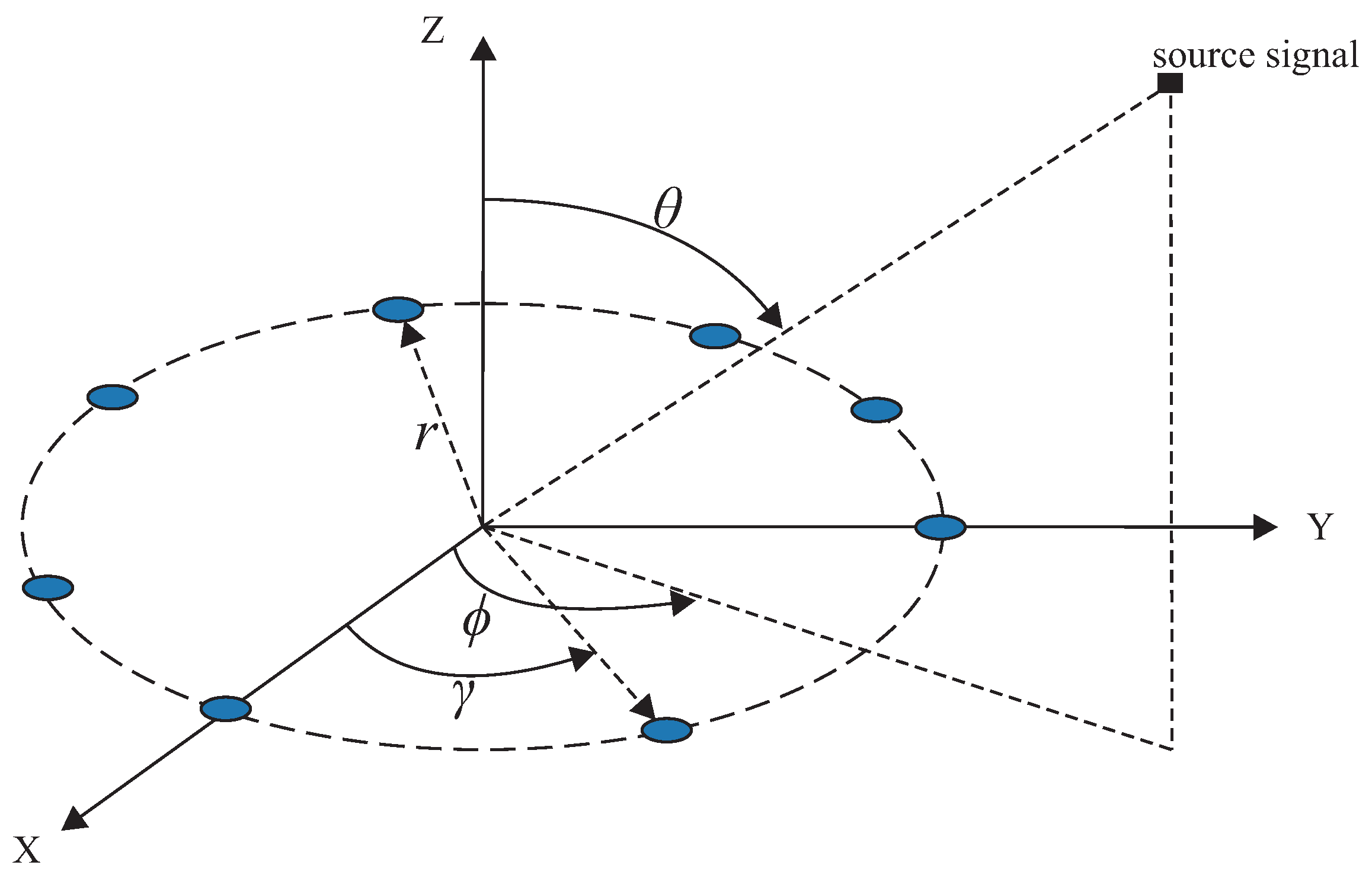
Figure 2.
The System Model.
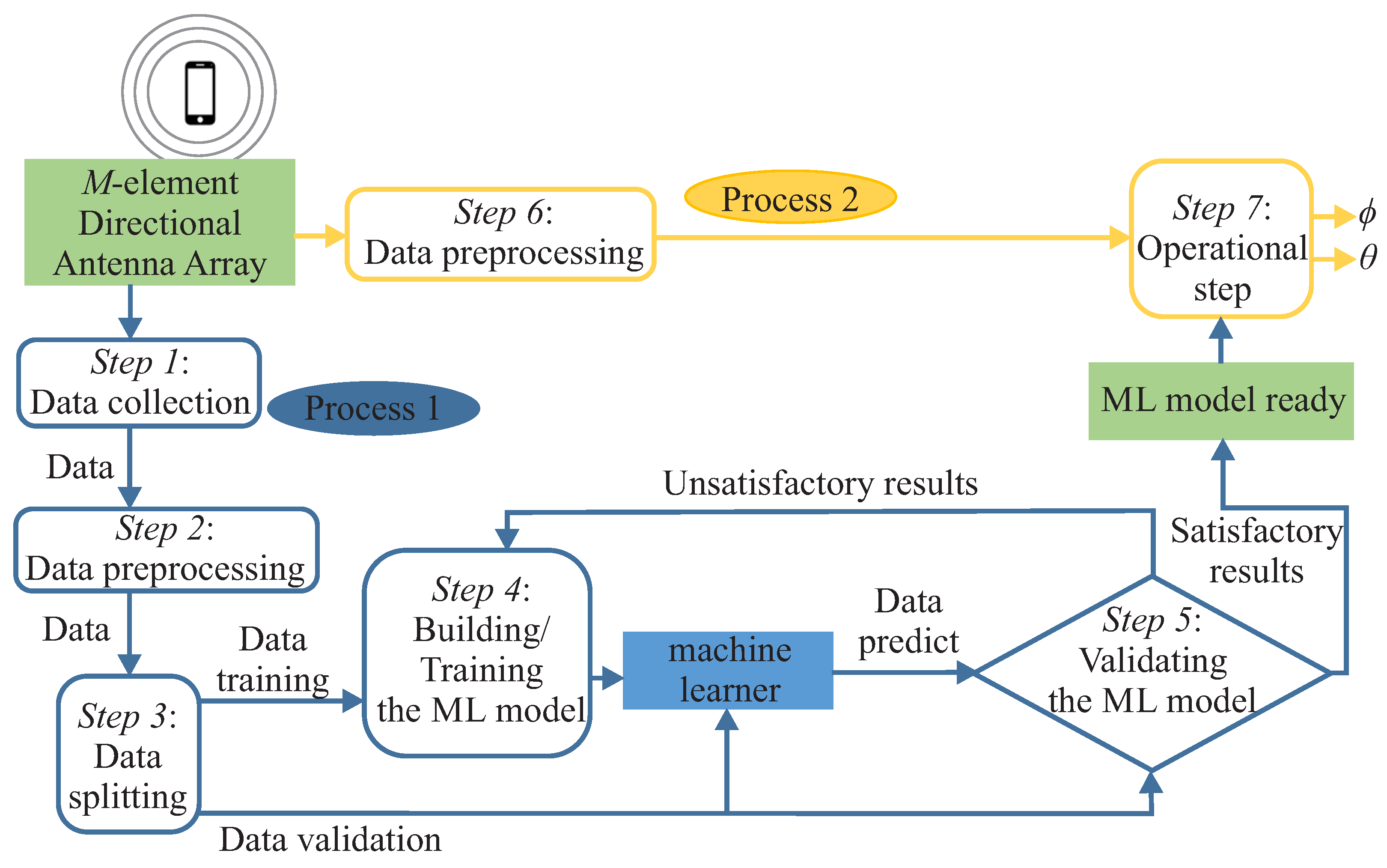
Figure 3.
Comparison of the RMSE for different numbers of receiving antennas: a) Azimuth and elevation angles’ RMSE versus SNR for different antenna numbers, b) Azimuth angle’s RMSE versus SNR for different antenna numbers, and c) Elevation angle’s RMSE versus SNR for different antenna numbers.
Figure 3.
Comparison of the RMSE for different numbers of receiving antennas: a) Azimuth and elevation angles’ RMSE versus SNR for different antenna numbers, b) Azimuth angle’s RMSE versus SNR for different antenna numbers, and c) Elevation angle’s RMSE versus SNR for different antenna numbers.
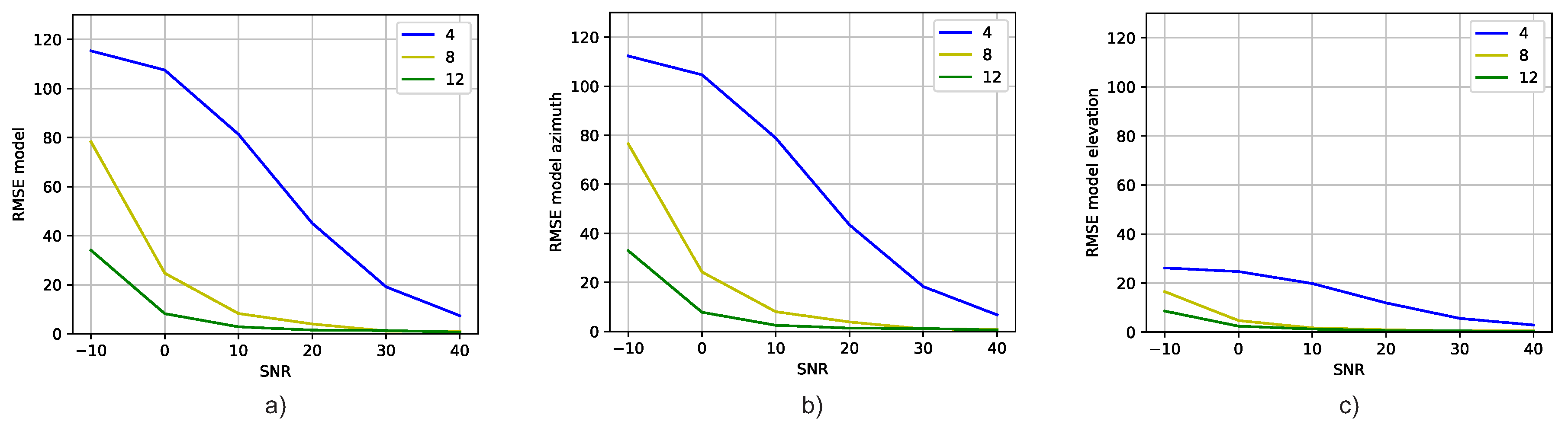
Figure 4.
SNR versus actual and predicted azimuth and elevation angles for different M (Experiment 1).
Figure 4.
SNR versus actual and predicted azimuth and elevation angles for different M (Experiment 1).
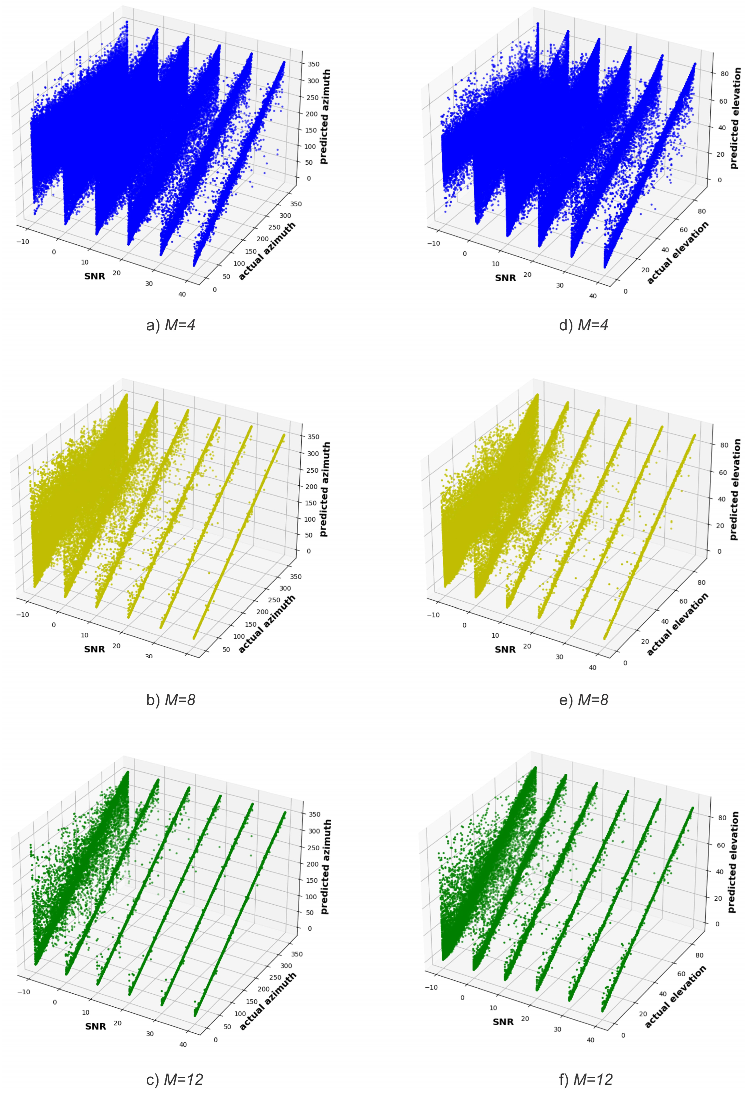
Figure 5.
Average RMSE of the DT models versus the SNR of the signals used to train the models.
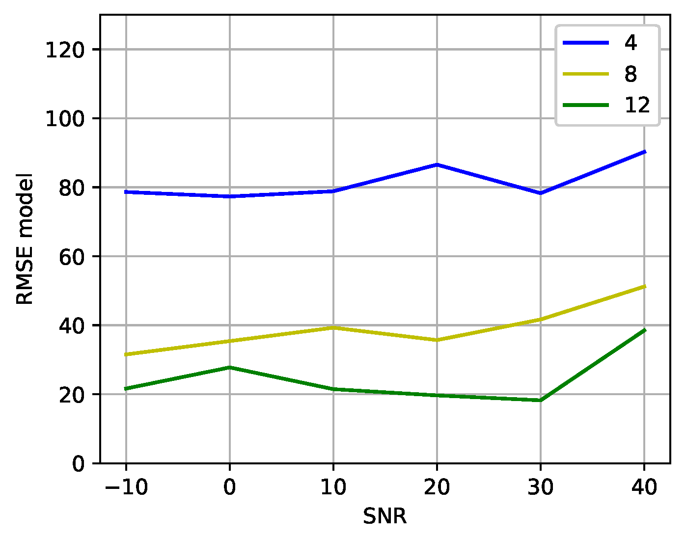
Figure 6.
Comparison of the RMSE of DT models trained with signals having an SNR of 20 dB versus the SNR of the signals used to validate them: a) Azimuth and elevation angles’ RMSE versus SNR for different antenna numbers, b) Azimuth angle’s RMSE versus SNR for different antenna numbers, and c) Elevation angle’s RMSE versus SNR for different antenna numbers.

Figure 7.
SNR versus actual and predicted azimuth and elevation angles for different M (Experiment 2).
Figure 7.
SNR versus actual and predicted azimuth and elevation angles for different M (Experiment 2).
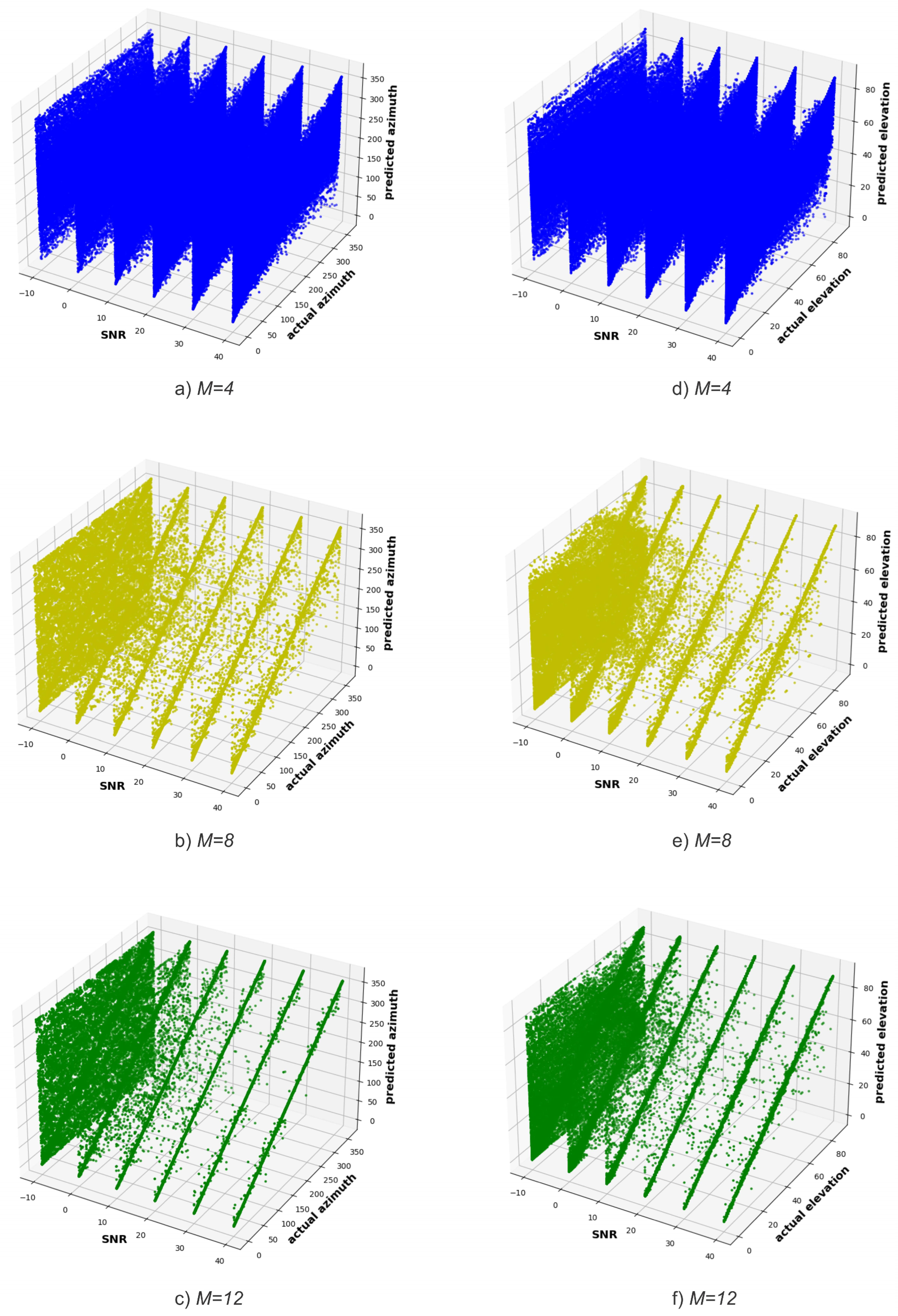
Figure 8.
RMSE vs. SNR for different antenna numbers: a) MUSIC, b) Experiment 1, c) Experiment 2.
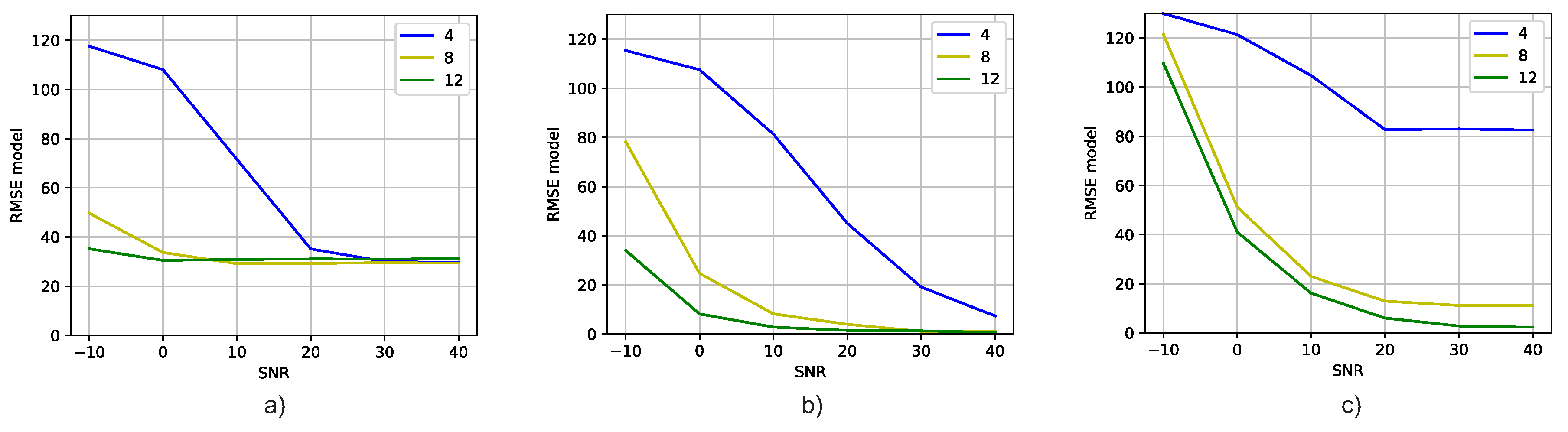
Figure 9.
Prediction time vs. SNR for different antenna numbers: a) MUSIC, b) Experiment 1, c) Experiment 2.
Figure 9.
Prediction time vs. SNR for different antenna numbers: a) MUSIC, b) Experiment 1, c) Experiment 2.
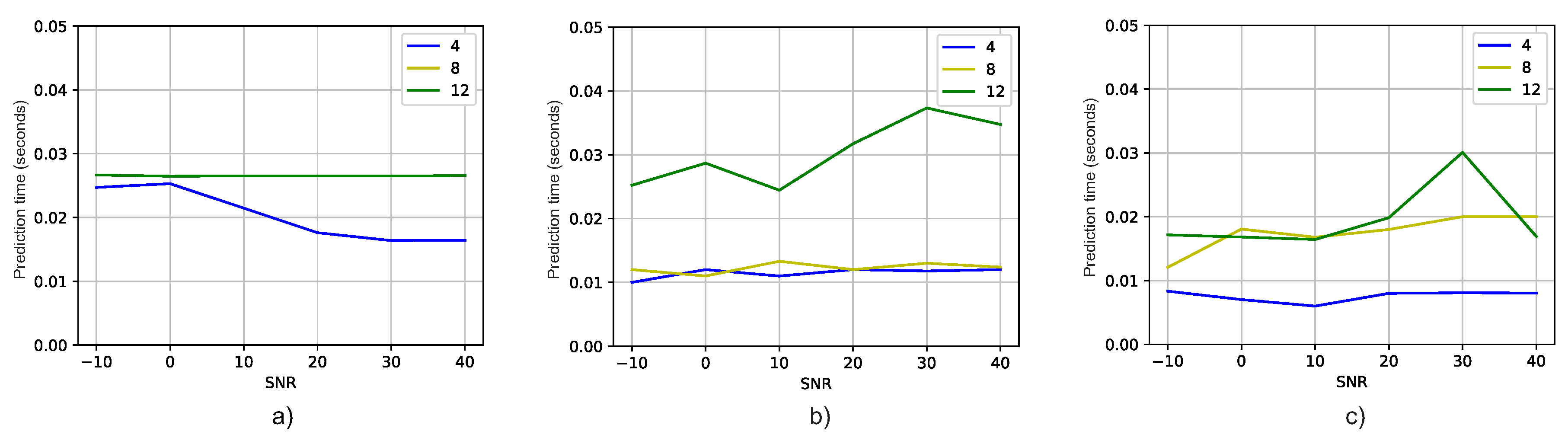

Table 1.
Taxonomy of the proposed ML to DOA estimation.
| Ref | Azimuth | Elevation | Single-source | Multi-source | Simulation | Experiment | Comparative with other works |
|---|---|---|---|---|---|---|---|
| [28] | x | x | x | x | x | ||
| [29] | x | x | x | x | x | ||
| [30] | x | x | x | ||||
| [31] | x | x | x | x | |||
| [32] | x | x | x | x | |||
| [33] | x | x | x | x | |||
| [34] | x | x | x | ||||
| [35] | x | x | x | x | x | ||
| [36] | x | x | x | x | |||
| [37] | x | x | x | x | x | ||
| [38] | x | x | x | x | x | ||
| [39] | x | x | x | x | x | x | |
| [40] | x | x | x | ||||
| [41] | x | x | x | x | |||
| [42] | x | x | x | x |
Table 2.
Summary of the best model hyperparameters for Experiment 1.
| Parameters | max_depth | min_samples_split | min_samples_leaf | splitter | criterion | max_features |
| Selection range | 100-1100, step: 100 | 2-40 | 1-40 | “best”, “random” | “friedman_mse”, “poisson” | “auto”, “log2”, “sqrt” |
| 500 | 27 | 19 | “best” | “friedman_mse” | “auto” | |
| 700 | 16 | 21 | “best” | “friedman_mse” | “log2” | |
| 1000 | 5 | 34 | “random” | “friedman_mse” | “auto” |
Table 3.
Summary of the best model hyperparameters for Experiment 2.
| Parameters | max_depth | min_samples_split | min_samples_leaf | splitter | criterion | max_features | |
| Selection range | 100-1100, step: 100 | 2-40 | 1-40 | “best”, “random” | “friedman_mse”, “poisson” | “auto”, “log2”, “sqrt” | |
| SNR = -10 dB | 400 | 16 | 34 | “best” | “friedman_mse” | “log2” | |
| 500 | 27 | 6 | “random” | “friedman_mse” | “sqrt” | ||
| 800 | 35 | 23 | “random” | “friedman_mse” | “sqrt” | ||
| SNR = 0 dB | 800 | 19 | 17 | “random” | “friedman_mse” | “auto” | |
| 100 | 3 | 12 | “random” | “friedman_mse” | “sqrt” | ||
| 900 | 28 | 24 | “random” | “friedman_mse” | “log2” | ||
| SNR = 10 dB | 600 | 7 | 13 | “best” | “friedman_mse” | “log2” | |
| 900 | 22 | 22 | “random” | “friedman_mse” | “log2” | ||
| 200 | 11 | 12 | “best” | “friedman_mse” | “log2” | ||
| SNR = 20 dB | 500 | 12 | 10 | “random” | “friedman_mse” | “sqrt” | |
| 200 | 39 | 9 | “random” | “friedman_mse” | “log2” | ||
| 400 | 22 | 8 | “best” | “friedman_mse” | “logs2” | ||
| SNR = 30 dB | 900 | 4 | 16 | “best” | “friedman_mse” | “log2” | |
| 1000 | 16 | 37 | “random” | “friedman_mse” | “log2” | ||
| 400 | 35 | 4 | “best” | “friedman_mse” | “sqrt” | ||
| SNR = 40 dB | 400 | 14 | 23 | “best” | “poisson” | “sqrt” | |
| 800 | 37 | 38 | “random” | “poisson” | “sqrt” | ||
| 100 | 34 | 25 | “random” | “poisson” | “sqrt” |
Disclaimer/Publisher’s Note: The statements, opinions and data contained in all publications are solely those of the individual author(s) and contributor(s) and not of MDPI and/or the editor(s). MDPI and/or the editor(s) disclaim responsibility for any injury to people or property resulting from any ideas, methods, instructions or products referred to in the content. |
© 2023 by the authors. Licensee MDPI, Basel, Switzerland. This article is an open access article distributed under the terms and conditions of the Creative Commons Attribution (CC BY) license (http://creativecommons.org/licenses/by/4.0/).
Copyright: This open access article is published under a Creative Commons CC BY 4.0 license, which permit the free download, distribution, and reuse, provided that the author and preprint are cited in any reuse.


