Submitted:
11 July 2023
Posted:
12 July 2023
You are already at the latest version
Abstract
The total tree height (h) and diameter at breast height (dbh) relationship is an essential tool in forest management and planning. The height—diameter (h-dbh) relationship had been studied with several approaches and for several species worldwide. The nonlinear mixed effect modeling (NLMEM) has been extensively used and lately the resilient backpropagation artificial neural network (RBPANN) approach has been a trend topic for modeling this relationship. The artificial neural network (ANN) is a computing system based in artificial intelligence and inspired in biological neural network for supervised learning. In this study the NLMEN and RBPANN approaches were used for modeling the h—dbh relationship for Durango pine species (Pinus durangensis Martínez) in mixed-species forest from Mexico. The total dataset considered 1,000 (11,472 measured trees) randomly selected from 14,390 temporary forest inventory plots and the dataset was randomly divided into two parts; 50% for training and 50% for testing. An unsupervised clustering analysis was used to grouped the dataset into 10 clusters based on k-means clustering method and plot-variables like density, basal area, mean dbh, mean h, quadratic mean diameter, altitude and aspect. The RBPANN was performed for tangent hyperbolicus (RBPANN-tanh), softplus (RBPANN-softplus), and logistic (RBPANN-logistic) activation functions for functions in cross product of the covariate or neurons and the weights for the ANN analysis. For both training and testing, 10 classical statistics (e.g., RMSE, R2, AIC, BIC, logLik) were computed for the residual values and assess the approaches for h—dbh relationship. For training and testing, the ANNs approach outperformed the NLMEM approach, and the RBPANN-tanh has the best performance in both training and testing phases.
Keywords:
artificial intelligence
; artificial neural network
; height-diameter relationship
; nonlinear mixed effect modeling
1. Introduction
Artificial Intelligence (AI) refers to the simulation of human intelligence in machines, wherein they are programmed to think and learn in a manner similar to humans. The AI has been used in forest modelling for different purposes and objectives. The machine learning (ML) is a subset of AI that focuses on the development of algorithms and models that enable computer to learns from a specific dataset and make predictions or take actions without being explicitly programmed [1,2]. One of the most ML techniques is the artificial neural network (ANN) and the resilient backpropagation artificial neural network (RBPANN) perform supervised ML in multi-layer perceptron, and the main principle is to eliminate the harmful influence of the size of the partial derivative on the weight step [3,4,5]. The ANNs are computational models inspired in the natural neurons and they represent a generalization of mathematical models of human cognition or neural biology [1,6,7]. In ANNs, the training and testing datasets are used to train and evaluate the performance of the network for a specific randomly selected dataset. The training dataset is used to train the neural network. It consists of a set of input data points and their corresponding target output values, while, the testing dataset is a separate dataset that is used to evaluate the performance of the trained neural network [1,8,9].
One of the most important relationships in forest modeling is the total tree height and diameter at breast height (h-dbh) relationship, and this relationship is usually applied in forest inventory or for height estimation in forest management and planning [10]. The knowledge of h-dbh relationship is a fundamental both developing and applying many growth and yield models [11,12]. This relationship has mainly studied with nonlinear mixed effect modeling (NLMEM) with fix and random parameters for several species and grouping level or ecological conditions [10,11,13,14,15,16]. Lately, this relationship has been studied with AI, and the ML thought ANN has been used [7,17,18]. Also, other variables as basal area [19], crown width [20], biomass [21], volume [22], forest fire [23], and annual radial growth with competition indices [24] have been studied with different ML algorithms. Occasionally, the clustering analysis based in unsupervised ML has been included in to group similar data point together based on their inherent characteristics or similarities [1,25,26,27]. The unsupervised clustering analysis could identify patterns or structures in dataset to improve the fitted models in forest modeling.
Specifically, in the Mexican Forestry the h-dbh relationship has been extensively studied with NLMEM for local and generalized models and occasionally the unsupervised cluster analysis was included in modelling [12,28,29]. The NLMEM are better than fitted models by ordinary least squares method and those use random parameter to explain the variability between groups, sites, or ecological regions. Lately, the ML algorithms are taken attention in forestry research and the results outperform the NLMEM approach for the h-dbh relationship. In ANN analysis is convenient to separate the dataset in two parts, one for training and other one for testing or validation [7,17]. The main used model for NLMEM has been th Chapman-Richards model [30], which is base in a sigmoid relationship growth based on age [31].
Considering the above schemes and the context of AI in forestry research, this study aim the h-dbh relationship for Durango Pine species (Pinus durangensis Martínez) by NLMEM and ANN for unsupervised clustered dataset for training and testing sets. The algorithms were compared in both training and testing phases and some conventional statistics like root mean square error, coefficient of determination, Akaike’s information criterion, Bayesian information criterion, and loglikelihood were uses to perform the approaches. The resilience backpropagation of ANN (RBPANN) was employed, and three activation functions were computed and evaluated. The activation functions were tangent hyperbolicus (RBPANN-tanh), softplus (RBPANN-softplus), and logistic (RBPANN-logistic), and those were trained by resilience backpropagation and maximum likelihood was used.
2. Materials and Methods
2.1. Study area
The study was developed in a forest community in Norther Mexico, specifically in Durango state. The forest community is called San Diego de Tezains, and the total area is around 61,098 ha, which 30,000 ha are used for forest management and timber harvesting. The main applied silvicultural treatments are based on continuous cover forestry (CCF) and rotation forest management (RFM) [32]. The silvicultural treatments for CCF area base on selection, while three thinning and shelterwood cutting treatments for RFM with 15-years of forest cycle cutting [33]. The location of study area is showed in Figure 1. The mean annual temperature ranges from 5 to 18 °C, and the lowest temperature occurs in January (− 6 °C) and the hottest in May (28 °C). The altitude varies from 1,500 to 3,033 m. The mixed-species stands are represented by seven genera: Pinus, Quercus, Juniperus, Cupressus, Pseudotsuga, Arbutus, and Alnus. The main species are Pinus durangensis Martínez and Quercus sideroxyla Bonpl. Lately, the Improve forest management combine the forest management and credit carbon offsets according to the Mexican Protocol developed by The Climate Action Reserve [34].
2.2. Dataset description
The dataset came from temporary forest inventory plots with a random sampling design for framework of 30,000 ha. A total of 14,390 temporary forest inventory plots were considered and Durango pine species was selected. A random sample of 1,000 plots was selected in sampling R package [35], and 11,472 measured trees were considered. Firstly, the unsupervised clustering analysis was used for grouping the dataset [1,25] according to the k-Means Clustering of kmeans R package [35]. Ten clusters were generated according with density (N, trees per hectare), basal area (BA, m2), mean diameter (Dm, cm), mean total tree (Hm, m), quadratic mean diameter (QMD, cm), altitudes (A, m), slope (S, %), and aspect (As, categorical variable). All variables were standardized, which perform values bounded 0.0 and 1.0 [21,36,37]. The standardization was performed according to Milligan and Cooper [38] and the Equation 1.
where Z is the standardized variable, x is the variable, Min and Max are the minimum and maximum values of x.
In the Clustering analysis, the cluster (k = 10) were generated, and the explained variance was 61.8812%. The data set is shown in Figure 2 for the total dataset and the clusters.
The site-specific variables for clustering analysis are recorded as a descriptive statistic in Table 1. All variables were standardized with Equation 1 to improve the clustering analysis [38].
The total dataset (11,472 pairs of h-dbh relationship) was randomly divided in two sets; 50% for training and 50% for testing or validation. The main statistics for both training and testing dataset are shown in Table 2 for the total tree height and diameter at breast height (h-dbh).
2.3. Nonlinear mixed effect modeling (NLMEM)
The base growth model developed by Richards [30] was used to model the nonlinear h-dbh relationship. This model is based on a sigmoid curve, and it is represented by Equation 2. This model had been extensively used in this kind of relationship [7,11,17,28].
where = total tree height j in the plot i; = lower asymptote parameter; , and = upper asymptote, growth rate, and slope of growth parameters; e = exponential function; = diameter at breast height j in the plot i; = residual j in the plot i. In this case for parameter, the value 1.3 was fixed. This warranted the total tree height equal to 1.3 m when diameter at breast height is equal to 0 mentioned by Fang and Bailey [39].
For NLMEM, the parameter vector of nonlinear model was defined according to Pinheiro, et al. [40] and summarize as follows [7,11,13] (Equation 3):
where is the vector of fixed parameters ( is the number of fixed parameters in the model), is the vector of random effect associated with cluster ( is the number of random parameters in the model), and and are the design matrices of size and ( is the total number of parameters in the model) for the fixed and random effects specific to each cluster. The residual vector (), and the random effect vector () are frequently assumed uncorrelated and normally distributed with mean zero and variance-covariance matrices and , respectively.
The upper asymptote parameter () was treated as a random parameter in the analysis for each cluster ( ), which explain about the maximum relationship between h and dbh. The random effect vector represent the variability between clusters for the asymptote parameter.
2.4. Artificial neural network (ANN)
The ANN are inspired by the early models of sensory processing by the brain. An ANN can easy be created by simulating a network of model neurons in a computer or specific programming language. Also, by applying mathematical algorithms that mimic the process of real neurons, we can make the network “learn” to solve many types of problems [41]. The ANNs can learn by themselves. Because of they have similarities with the information processing features of the human brain (nonlinearity, high parallelism, capability to generalize), this modeling technique has the potential ability to solve problems that are difficult to formalize, such as problems of biological nature [7,41]. The resilient backpropagation artificial neural network (RBPANN) is a logical adaptative learning scheme, which perform supervised batch learning in multi-layer perceptron. The basic principle of RBPANN is to eliminate the harmful influence of the size of the partial derivative on the weight steps [3,4,19].
According to Barbosa, Costa, Schons, Finger, Liesenberg and Bispo [19], and Anastasiadis, et al. [42], the RBP for ANN employs a sign-based scheme to update the weights in order to eliminate harmful influences of the derivatives´ magnitude on the weight updates. The size of the update step along a weight direction is exclusively determined by a weight-specific “update-value” as follows:
where denotes the partial derivative of bathc error with respect to weight at the kth iteration.
The second step of RBP learning is to determine the new update values [19], as follows:
where .
The total number of parameters in RBPANN is five; (i) the increase factor isa set to ; (ii) the decrease facto is set to ; (iii) the initial updates-value is set to : (iv) the maximum step; (v) the minimum steps.
According to Cartwright [43], the first step in using ANNs is to determine a suitable topology, optimal if possible (number of inputs and outputs, number of hidden layers, and neurons in each layer) and optimal (weights, biases, and activation functions). The process of ANNs begins by setting up the weights as small random variables. Then, each input pattern undergoes a feedforward phase, where the input signal is received and transmitted to all nodes in the hidden layer. In ANNs, every hidden node calculates the sum of its weighted input signals, applies an activation function to determine its output signal, and transmits this signal to the output node. At the output node, the final output signal is computed using the received signals from the hidden nodes [7]. Within the context of RBPANN, the associated error () is computed, and this error is utilized to adjust the weights. The weights correction term is determined based on the error, and it is subsequently employed to update the corresponding weights. Additionally, the is transmitted to each hidden node. Each hidden node then calculates its error information term by summing the inputs received from the output node, multiplied by the derivative of its activation function [7,43,44]. According to Fausett [45] and Cartwright [43], the general formulation for RBPANN could be as follows (Equation 6):
where is the bias on output unit , is the learning rate, is the ratio of error correction weight fitted for that is due to an error at output , also the information about the error at unit that is propagated back to the hidden units that feed into unit , is the output activation of the hidden unit and is the momentum parameter (refers to the contribution of the gradient calculated at the previous time step to the correction of the weights) [43].
The used activation functions for smoothing the h-dbh relationship through RBPANN were tangent hyperbolicus (RBPANN-tanh), softplus (RBPANN-softplus), and logistic (RBPANN-logistic) functions [4,42], these activation functions occur between the hidden layers or between the input layer and hidden layer [17]. These functions were defined for RBPANN-tanh, RBPANN-softplus, and RBPANN-logistic in Equations 7, 8, and 9, respectively. Also, the derivatives are in Equations 10, 11 and 12, respectively.
where is the information of the node transmits, in which are the weights and are the input values with , , and for RBPANN-tanh, RBPANN-softplus, and RBPANN-logistic, respectively.
In the ANN learning process, a different vector from 1 to 10 for each hidden layer was performed in a preliminary analysis, and the best results were obtained when the vector was 10 nodes for each hidden layer c(10, 10, 10). In Figure 3, the ANNs plot are presented for vectors c(3, 3, 3), c(5, 5, 5), and c(10, 10, 10) in the hidden layer.
For both RBPANN-tanh and RBPANN-logistic functions, the topology was as follows: (i) two inputs (dbh and cluster); (ii) one output (h); (iii) a vector c(10, 10, 10) hidden layers; and (iv) two nodes for the first layer, 11 nodes for the second, third and fourth layer layers (Bias node is included) and two nodes for the fifth layer. The ANNs for RBPANN-tanh, RBPANN-softplus, and RBPANN-logistic activation functions are presented in Figure 4. Input variables are represented by “I” in nodes, hidden nodes are represented by “H”, input variable is represented by "O”, and Bias nodes are represented by “B”.
For RBPANN-tanh, RBPANN-softplus, and RBPANN-logistic activation functions. The number of repetitions was 10, the maximum steps for training of the NN was 107 , and the threshold was 0.1, which is similar that arguments used by Özçelik, Diamantopoulou, Crecente-Campo and Eler [7] and Shen, Hu, Sharma, Wang, Meng, Wang, Wang and Fu [17]. Also, the training algorithm for ANNs was the resilient backpropagation with weight backtracking [4,42,43]
2.5. Fitting modeling
For NLME, the total tree height and diameter at breast height (h-dbh) relationship was fitted in “nlme” R package [35] and used maximum likelihood estimation method [40] for fixed and random parameters withing cluster groups. While for ANN models, the “neuralnet” R package [35] was used. For ANN, the resilient backpropagation (RPROP) for tangent hyperbolicus (tanh), softplus (softplus), and logistic (logistic) functions were programed for smoothing the result of the cross product of the covariate or neurons and the weights [3,4,45]. All functions about fitting statistics for both training and testing were programmed in R environment [35].
2.6. Models performance criteria
For both training and testing steps, the fitting statistics were obtained in two levels, first one for the entire dataset and second one for each cluster. The statistics were the root mean square error (RMSE), standard error of estimate (SEE), relative SEE (RSEE), fitting index (FI), mean error (E), relative E (RE), Akaike information criterion (AIC), Bayesian information criterion (BIC) and the log-likelihood (logLik). The statistics were computed as follows:
where , and are observed, predicted and average values of h variable; n = observations; p = number of parameters estimated; and log = logarithm function.
In all cases, the residual values were obtained with the implementation of NLMEM or RBPANN models and the statistics were programmed in R environment [35]. Lately, the NLMEM and ANNs models were ranked based on the overall dataset and cluster-group for all fitting statistics. A ranking system of Kozak and Smith [46] was used. All fitted statistics were equally weighted and Rank 1 was used for the best model and 4 for the poorest.
3. Results
3.1. Training phase
3.1.1. NLMEM
The fitted growth equation for h-dbh relationship by NLMEM performed well and all parameters were significantly different to zero at 5% of significance level. The relationship between total tree height and diameter at breast height can be explained with fixed and random parameters. In Table 3, the estimated parameters and their statistical properties can be found for the entire training dataset. Furthermore, the confidence interval for each parameter is recorded at a 95% confidence level.
The training phase's fitting statistics are presented in Table 4, which includes the overall training dataset as well as the cluster-groups individually. For both overall training dataset, and cluster-groups, the fitting statistics were accurate and showed the potential to offer the NLMEM approach for the h-dbh relationship. The RMSE value for the overall training dataset was 3.1085 m, the best value was 2.4735 for cluster-group 1 (C1) and the worst value for cluster-group 4 (C4). Additionally, the overall training dataset exhibited an E value of -0.0005. The highest value was observed in C3, indicating the poorer performance, while the lowest value was found in C4, indicating the best performance. In terms of AIC, the C4 demonstrated the best performance, whereas C6 exhibited relatively poorer performance.
3.1.1. RBPANN
The results about performed ANNs for RBPANN-tanh, RBPANN-softplus, and RBPANN-logistic activation functions are shown in Table 5. The statistics are in standardized variables and observed in 10 repetitions in the learning process. In this scenario, all three activation functions exhibit favorable outcomes. Specifically, both RBPANN-tanh and RBPANN-softplus deliver comparable performance. In contrast, RBPANN-logistic exhibited the lowest performance among the three activation functions. Additionally, the RBPANN-logistic achieved the minimum number of steps (88) required for convergence.
The fitting statistics for three ANNs applied to examine the h-dbh relationship in Durango pine are presented for both the overall dataset and each cluster-group in Table 6 for training phase. The nine fitting statistics illustrate the accuracy of RBPANN-tanh, RBPANN-softplus, and RBPANN-logistic activation functions in the ANNs models. The topology of each ANN, as depicted in Figure 4, exhibited satisfactory results in predicting h based on dbh and an unsupervised clustering analysis for ten groups. Overall, the estimations demonstrate similar characteristics across the three activation models. However, RBPANN-tanh exhibits certain advantages that are comparable to the other activation functions in the training phase. All ANNs were trained using the resilience backpropagation learning algorithm, and the likelihood function was employed.
The residual and predicted values are presented in Figure 5 for each cluster-group by RBPANN-tanh, which was the best approach in training phase to model the h-dbh relationship. In general, the residuals ranged between -6 m and 6 m. Enhancing the training phase could involve increasing the number of repetitions or epochs, however, the computational process ought to be significantly time-consuming.
Finally, The ranks and sums of ranks for hierarchy of NLMEN and ANNs are presented in Table 7. The statistics for both the overall dataset and the cluster-group were ranked from 1 to 4. In terms of the overall dataset, the RBPANN-softplus exhibited the best performance during the training phase, which was comparable to the NLMEN model and other ANNs. The RBPANN-tanh activation function ranked second, while the RBPANN-logistic ranked third. On the other hand, the NLMEN approach had the lowest rank sum, indicating poorer performance compared to the other models. A similar pattern was observed within the cluster-groups, and the sum of ranks resulted in the following rankings: 176, 241, 269, and 304 for RBPANN-tanh, RBPANN-softplus, NLMEN, and RBPANN-logistic, respectively. It is worth noting that only the RBPANN-logistic demonstrated lower performance compared to the NLMEN approach. The number in parenthesis indicate the ranking for models in the overall dataset.
3.1. Testing or Validation phase
3.1.1. NLMEM
During the testing phase, 5,736 pairs of heights and diameters from 50% of the dataset were utilized. Height estimations were performed using fixed and random parameters for each cluster-group provided by NLMEM approach. The nine testing statistics were computed at two levels: for the overall dataset and for each cluster-group. The Table 8 presents the statistics for testing the advantages of NLMEN for overall dataset and for each cluster-group. All the statistics displayed satisfactory performance, which depended on the number of observations. Additionally, the cluster-groups with limited information exhibited the lowest values. Among the cluster-groups, C4 had the maximum number of observations, whereas C9 had the minimum number of observations.
3.1.1. RBPANN
During the testing phase, the results for the ANNs were similar to the training phase. The ANN utilizing the tangent hyperbolicus activation function (RBPANN-tanh) exhibited the highest performance, followed by RBPANN-logistic, and finally RBPANN-softplus. The Table 9 records the statistics for the testing dataset, both in the overall dataset and within each cluster-group. The FIs values for the overall dataset were higher than 0.7029, when RBPANN-tanh demonstrating the best performance and RBPANN-logistic exhibiting the poorest performance. A similar pattern was observed for other statistics such as AIC BIC and logLik. Furthermore, in this instance, the ANNs demonstrate superior performance compared to the NLMEM approach.
The Figure 6 displays the representation of residual and predicted values for each cluster-group obtained through RBPANN-tanh. In this scenario, the residual dispersion appears to be larger compared to the training phase. However, this can be attributed to the utilization of a new dataset, where the predictions are made under different training conditions. Cluster-groups 4 and 10 exhibited higher levels of dispersion compared to the remaining cluster-groups.
Finally, the ranks and sums of ranks for hierarchy of NLMEN and ANNs are presented in Table 10. During the testing phase, the RBPANN-tanh achieved the highest rank of 1 with a sum of ranks of 9, while the NLMEM approach performed the poorest, ranking 4 with sum of ranks of 36. The RBPANN-softplus and RBPANN-logistic exhibited relatively similar performance conditions. Among the proven models of ANNs, the RBPANN-logistic exhibited the poorest performance. In terms of the sum of ranks for the combined overall dataset and cluster-groups, the RBPANN-tanh demonstrated the best performance with a sum of ranks of 181. Following that, the RBPANN-logistic, RBPANN-softplus, and NLMEM were ranked 2nd, 3rd, and 4th, with sum of ranks of 201, 240, and 368, respectively.
4. Discussion
Having knowledge about the total tree height and diameter at breast height is essential for both the development and application of many growth and yield models. Models focusing on the h-dbh relationship serve as valuable tools for accurately predicting tree height based on dbh measurements. Because of the dbh can be conducted quickly, easily, and accurately, but the measurement of total tree height is comparatively complex, time consuming, and expensive [11]. The NLME had been a capable approach to generate models in h-dbh relationship for different species and assumed fixed and random parameters for specific-groups or covariables to study the variability inter-and intra-plots, ecological regions or cluster-groups [10,16,39]. Also, these models have been studied for local and generalized formulations with NLMEM approach [12,13,16,28]. In this case of study the NLMEM performance was accurately strong to model the h-dbh relationship for Durango pine and the inclusion of unsupervised clustering analysis improve the estimated parameters and its statistics properties [36,47], which involve fixed parameter for the overall dataset in training phase and random parameter for each cluster-group, also parameter to give information about general variability and variability within cluster-group.
The NLMEM demonstrated outstanding performance during the training phase, with the fitting process converging quickly and effortlessly. Additionally, the maximum likelihood approach yielded favorable and suitable results particularly when expressing the asymptote parameter with mixed effects (Table 3 and Table 4). All parameters in fitting process were significantly different to zero at 5% of significance level and the random parameters allow suitable estimations in training phase and those were used for cluster-groups in testing phase. The application of the NLMEM approach on the testing dataset resulted in successful outcomes that aligned with the expected results (as shown in Table 8), accompanied by the utilization of appropriate statistical measures. As an illustration, the root mean square error (RMSE) for the overall dataset during the testing phase was determined to be 3.1438 m, with an average value of 3.3773 m observed within the cluster-groups (refer to Table 8). By employing a mixed-effect model and incorporating cluster-group inclusion, the Chapman-Richards growth equation [30] (Equation 2) proves to be a highly effective model for predicting the height of Durango pine trees. Similar results have been conducted for several species an different conditions [11,16,28]. Even though the NLMEM method is accurate for height prediction based on diameter measurements, it is worth considering that ANNs could be a suitable alternative for modeling the h-dbh relationship under several dataset conditions and the incorporation of grouped strategies [7,14,48]. In recent times, there has been a growing application of AI and ML techniques in the fields of biology and forestry. These advanced approaches have proven valuable in addressing challenges that require substantial computational resources and unsupervised learning methods [1,41], Several of these approaches have been employed in studying the height-diameter at breast height (h-dbh) relationship, leading to notable outcomes and reported successes for various species and under diverse forest management conditions, demonstrating their versatility and effectiveness [7,14,15,17,48]. In this context the ANNs model outperformed the NLMEM approach.
In this study, the ANNs were evaluated and compared with the traditional NLMEM method. The ANNs utilized the RBP learning algorithm along with three activation functions. In most cases, the ANNs employing RBPANN-tanh, RBPANN, and RBPANN-logistic (Equations 7, 8, an 9, respectively) exhibited superior performance compared to the results obtained by NLMEM, both during the training and testing phases. The training statistics for three ANNs, as presented in Table 6, exhibited enhanced fitting performance compared to the statistics obtained by NLMEM (see Table 4). This improvement was observed in both the overall dataset and cluster-group analyses. These findings provide evidence that the clustering analysis using the k-means algorithm effectively grouped the dataset utilized in this study [36,47]. The RBPANN-tanh model, employing a tangent hyperbolic activation function, demonstrated the highest performance in predicting height measurements during both the training and testing phases (it can see in Table 6 and 9). Furthermore, the ranks and sum of ranks, based on the ranking system proposed by Kozak and Smith [46], provided evidence of the advantages of the ANNs models over the NLMEM approach. Models such as RBPANN-logistic were reported by Özçelik, Diamantopoulou, Crecente-Campo and Eler [7] revealed that models such as RBPANN-logistic exhibited advantages over NLMEM models when predicting the growth of Crimean juniper in the southern and southwestern regions of Turkey. Conversely Shen, Hu, Sharma, Wang, Meng, Wang, Wang and Fu [17] developed ANNs models utilizing RBPANN-logistic and RBPANN-tanh transfer or activation functions for Populus spp. L. in China, where the RBPANN-logistic model outperformed both the NLMEN and the RBPANN-tanh model. In our case, the best ANN was the RBPANN-tanh and this outperformed other tested ANNs and NLMEM approach. Similar results have been reported the advantages of ANNs or deep learning algorithms over the ordinary least square and NLMEM models in both training and testing or validation phases [14,15,48,49]. In all cases, the implementation of ANNs exhibited significant advantages over traditional approaches when modeling the h-dbh relationship.
In this study, based on the implemented ranking system, the RBPANN-tanh model emerged as the top performer (residual and predicted values are showed in Figure 5 and Figure 6). It achieved a sum of ranks of 176 for the training phase and 81 for the testing phase. These sums of ranks account for both the overall dataset and cluster-groups, as illustrated in Table 7 and Table 10, respectively. In terms of training, the RBPANN-softplus model ranked second, whereas during the testing phase, the RBPANN-logistic model exhibited the second-best performance. On the other hand, the RBPANN-logistic model performed least effectively in the training phase, while the NLMEM model demonstrated comparatively lower performance during the testing phase. The ANNs developed in this study, as depicted in Figure 4, were trained using the RBP algorithm. The ANNs were then evaluated using three different activation functions: RBPANN-tanh, RBPANN-softplus, and RBPANN-logistic. These models comprised a total of five layers, including three hidden layers. The training process involved ten repetitions to ensure robustness and accuracy. Even though the RBPANN-logistic converging in 88 steps, it exhibited relatively poorer performance compared to the RBPANN-tanh, which achieved better results within 301 steps. Interestingly, the RBPANN-logistic required a longer convergence time of 1885 steps, indicating its comparatively poorer performance in this aspect. As a result, the developed ANNs model showcased a high capability for predicting total tree height measurements. This highlights the potential application of AI in modeling the h-dbh relationship, not only for Durango pine but also for general forest modeling purposes or other variables [6,19,21,50]. The ANNs could be used to improve the estimations in forest inventory and forest management and planning in mixed-species forest in Durango, Mexico.
5. Conclusions
The nonlinear mixed effect modeling (NLMEM) and Artificial Neural Networks (ANN) with resilience backpropagation (RBP) were employed to model the height-diameter at breast height (h-dbh) relationship for Durango pine species. Unsupervised clustering analysis was conducted to enhance the capability of the trained and tested models.. Three activation functions, namely tangent hyperbolicus (RBPANN-tanh), softplus (RBPANN-softplus), and logistic (RBPANN-logistic), were utilized in RBPANN. Those activation functions were trained and tested on both overall dataset and each cluster group. In general, the ANNs outperformed the NLMEM for predictions of heights in training and testing phases. The best model in both training and testing phases was the RBPANN-tanh, which assumed five layers in the ANN and three of them were hidden. The use of ANNs proves to be a suitable and effective approach for estimating the total tree height of Durango pine species. Additionally, incorporating unsupervised clustering analysis enhances the estimation accuracy in ANN models, highlighting the capabilities of artificial intelligence (AI) in this context. In conclusion, AI techniques such as ANNs prove to be suitable and modern statistical tools for forest modeling.
Author Contributions
Conceptualization, G.Q.B. and Y.O.; methodology, G.Q.B. and Y.O.; validation, G.Q.B., and Y.O.; formal analysis, G.Q.B., and Y.O..; investigation, G.Q.B., and Y.O.; resources, G.Q.B.; writing—original draft preparation, G.Q.B., and Y.O.; writing—review and editing, G.Q.B., and Y.O.; visualization, G.Q.B; supervision, G.Q.B.; project administration, G.Q.B.; funding acquisition, Y.O. All authors have read and agreed to the published version of the manuscript.
Funding
This research was funded by Guangdong Science and Technology Department Project.
Data Availability Statement
Not applicable.
Acknowledgments
The authors of this article express their gratitude to Ejido San Diego de Tezains community in Durango, Mexico for data supporting.
Conflicts of Interest
The authors declare no conflict of interest.
References
- Wodecki, A. Artificial Intelligence Methods and Techniques. In Artificial Intelligence in Value Creation; Wodecki, A., Ed. Springer International Publishing: Cham, 2019. [CrossRef]
- Holzinger, A.; Keiblinger, K.; Holub, P.; Zatloukal, K.; Müller, H. AI for life: Trends in artificial intelligence for biotechnology. New Biotechnology 2023, 74, 16–24. [Google Scholar] [CrossRef]
- Riedmiller, M.; Braun, H. A direct adaptive method for faster backpropagation learning: The RPROP algorithm; 0780309995; IEEE, 1993; pp. 586–591. [Google Scholar]
- Riedmiller, M.; Braun, H. Rprop-description and implementation details; Technical Report. Univer, 1994. [Google Scholar]
- Hecht-Nielsen, R. Hecht-Nielsen, R. III.3 - Theory of the Backpropagation Neural Network**Based on “nonindent” by Robert Hecht-Nielsen, which appeared in Proceedings of the International Joint Conference on Neural Networks 1, 593–611, June 1989. © 1989 IEEE. In Neural Networks for Perception; Wechsler, H., Ed. Academic Press, 1992. [Google Scholar] [CrossRef]
- Chen, W.; Shirzadi, A.; Shahabi, H.; Ahmad, B.B.; Zhang, S.; Hong, H.; Zhang, N. A novel hybrid artificial intelligence approach based on the rotation forest ensemble and naïve Bayes tree classifiers for a landslide susceptibility assessment in Langao County, China. Geomatics, Natural Hazards and Risk 2017, 8, 1955–1977. [Google Scholar] [CrossRef]
- Özçelik, R.; Diamantopoulou, M.J.; Crecente-Campo, F.; Eler, U. Estimating Crimean juniper tree height using nonlinear regression and artificial neural network models. Forest Ecology and Management 2013, 306, 52–60. [Google Scholar] [CrossRef]
- Russell, S.J. Artificial intelligence a modern approach; Pearson Education, Inc., 2010. [Google Scholar]
- Gui, Y.; Li, D.; Fang, R. A fast adaptive algorithm for training deep neural networks. Applied Intelligence 2023, 53, 4099–4108. [Google Scholar] [CrossRef]
- Mehtätalo, L.; de-Miguel, S.; Gregoire, T.G. Modeling height-diameter curves for prediction. Canadian Journal of Forest Research 2015, 45, 826–837. [Google Scholar] [CrossRef]
- Sharma, M.; Parton, J. Height–diameter equations for boreal tree species in Ontario using a mixed-effects modeling approach. Forest Ecology and Management 2007, 249, 187–198. [Google Scholar] [CrossRef]
- Santiago-García, W.; Jacinto-Salinas, A.H.; Rodríguez-Ortiz, G.; Nava-Nava, A.; Santiago-García, E.; Ángeles-Pérez, G.; Enríquez-del Valle, J.R. Generalized height-diameter models for five pine species at Southern Mexico. Forest Science and Technology 2020, 16, 49–55. [Google Scholar] [CrossRef]
- Szurszewski, J.H. Mechanism of action of pentagastrin and acetylcholine on the longitudinal muscle of the canine antrum. J Physiol 1975, 252, 335–361. [Google Scholar] [CrossRef] [PubMed]
- Elliott, R.J.; Gardner, D.L. Proline determination with isatin, in the presence of amino acids. Anal Biochem 1976, 70, 268–273. [Google Scholar] [CrossRef] [PubMed]
- Ogana, F.N.; Ercanli, I. Modelling height-diameter relationships in complex tropical rain forest ecosystems using deep learning algorithm. Journal of Forestry Research 2021, 33, 883–898. [Google Scholar] [CrossRef]
- Raptis, D.I.; Kazana, V.; Kazaklis, A.; Stamatiou, C. Mixed-effects height–diameter models for black pine (Pinus nigra Arn.) forest management. Trees 2021, 35, 1167–1183. [Google Scholar] [CrossRef]
- Shen, J.; Hu, Z.; Sharma, R.P.; Wang, G.; Meng, X.; Wang, M.; Wang, Q.; Fu, L. Modeling height–diameter relationship for poplar plantations using combined-optimization multiple hidden layer back propagation neural network. Forests 2020, 11, 442. [Google Scholar] [CrossRef]
- Diamantopoulou, M.J. Predicting fir trees stem diameters using Artificial Neural Network models. The Southern African Forestry Journal 2005, 205, 39–44. [Google Scholar] [CrossRef]
- Barbosa, L.O.; Costa, E.A.; Schons, C.T.; Finger, C.A.G.; Liesenberg, V.; Bispo, P.d.C. Individual Tree Basal Area Increment Models for Brazilian Pine (Araucaria angustifolia) Using Artificial Neural Networks. Forests 2022, 13, 1108. [Google Scholar] [CrossRef]
- Qin, Y.; Wu, B.; Lei, X.; Feng, L. Prediction of tree crown width in natural mixed forests using deep learning algorithm. Forest Ecosystems 2023, 10, 100109. [Google Scholar] [CrossRef]
- Vahedi, A.A. Artificial neural network application in comparison with modeling allometric equations for predicting above-ground biomass in the Hyrcanian mixed-beech forests of Iran. Biomass and Bioenergy 2016, 88, 66–76. [Google Scholar] [CrossRef]
- Diamantopoulou, M.J.; Milios, E. Modelling total volume of dominant pine trees in reforestations via multivariate analysis and artificial neural network models. Biosystems Engineering 2010, 105, 306–315. [Google Scholar] [CrossRef]
- Wu, Z.; Wang, B.; Li, M.; Tian, Y.; Quan, Y.; Liu, J. Simulation of forest fire spread based on artificial intelligence. Ecological Indicators 2022, 136, 108653. [Google Scholar] [CrossRef]
- Richards, M.; McDonald, A.J.S.; Aitkenhead, M.J. Optimisation of competition indices using simulated annealing and artificial neural networks. Ecological Modelling 2008, 214, 375–384. [Google Scholar] [CrossRef]
- Öhman, K.; Lämås, T. Clustering of harvest activities in multi-objective long-term forest planning. Forest Ecology and Management 2003, 176, 161–171. [Google Scholar] [CrossRef]
- Akay, A.O.; AKGÜL, M.; Esin, A.I.; Demir, M.; ŞENTÜRK, N.; ÖZTÜRK, T. Evaluation of occupational accidents in forestry in Europe and Turkey by k-means clustering analysis. Turkish Journal of Agriculture and Forestry 2021, 45, 495–509. [Google Scholar] [CrossRef]
- Phillips, P.D.; Yasman, I.; Brash, T.E.; van Gardingen, P.R. Grouping tree species for analysis of forest data in Kalimantan (Indonesian Borneo). Forest Ecology and Management 2002, 157, 205–216. [Google Scholar] [CrossRef]
- Corral-Rivas, S.; Álvarez-González, J.; Crecente-Campo, F.; Corral-Rivas, J. Local and generalized height-diameter models with random parameters for mixed, uneven-aged forests in Northwestern Durango, Mexico. Forest Ecosystems 2014, 1, 6. [Google Scholar] [CrossRef]
- Castillo-Gallegos, E.; Jarillo-Rodríguez, J.; Escobar-Hernández, R. Diameter-height relationships in three species grown together in a commercial forest plantation in eastern tropical Mexico. Revista Chapingo serie ciencias forestales y del ambiente 2018, 24, 33–48. [Google Scholar] [CrossRef]
- Richards, F.J. A Flexible Growth Function for Empirical Use. Journal of Experimental Botany 1959, 10, 290–300. [Google Scholar] [CrossRef]
- Burkhart, H.E.; Tomé, M. Modeling forest trees and stands; Springer Science & Business Media, 2012. [Google Scholar]
- Von Gadow, K.; Nagel, J.; Saborowski, J. Continuous cover forestry: assessment, analysis, scenarios; Springer Science & Business Media, 2002; Volume 4. [Google Scholar]
- Quiñonez-Barraza, G.; Zhao, D.; De Los Santos Posadas, H.M.; Corral-Rivas, J.J. Considering neighborhood effects improves individual dbh growth models for natural mixed-species forests in Mexico. Annals of forest science 2018, 75, 1–11. [Google Scholar] [CrossRef]
- Climate Action Reserve [CAR]. Protocolo Forestal para México. Versión 3.0. CA, USA. Climate Action Reserve: 2022; Vol. Versión 3.0, p 2080 p.
- R Core Team. A language and environment for statistical computing. Vienna, Austria: R Foundation for Statistical Computing; 2012. https://www.r-project.org/ 2023.
- Ghoshal, S.; Nohria, N.; Wong, M. A K-means clustering algorithm. Algorithm AS 136. Applied Statistics 1979, 28, 100–108. [Google Scholar]
- Forgy, E.W. Cluster analysis of multivariate data: Efficiency vs. interpretability of classifications. biometrics 1965, 21, 768–769. [Google Scholar]
- Milligan, G.W.; Cooper, M.C. A study of standardization of variables in cluster analysis. Journal of Classification 1988, 5, 181–204. [Google Scholar] [CrossRef]
- Fang, Z.; Bailey, R.L. Height–diameter models for tropical forests on Hainan Island in southern China. Forest Ecology and Management 1998, 110, 315–327. [Google Scholar] [CrossRef]
- Pinheiro, J.C.; Bates, D.M.; Lindstrom, M.J. Model building for nonlinear mixed effects models; University of Wisconsin, Department of Biostatistics Madison, WI, 1995. [Google Scholar]
- Krogh, A. What are artificial neural networks? Nat Biotechnol 2008, 26, 195–197. [Google Scholar] [CrossRef] [PubMed]
- Anastasiadis, A.D.; Magoulas, G.D.; Vrahatis, M.N. New globally convergent training scheme based on the resilient propagation algorithm. Neurocomputing 2005, 64, 253–270. [Google Scholar] [CrossRef]
- Cartwright, H. Artificial neural networks: Methods in Molecular Biology, Third Edition. New Yor, NY USA ed.; Springer Human Press: New Yor, NY USA, 2021. [Google Scholar]
- Han, W.; Nan, L.; Su, M.; Chen, Y.; Li, R.; Zhang, X. Research on the prediction method of centrifugal pump performance based on a double hidden layer BP neural network. Energies 2019, 12, 2709. [Google Scholar] [CrossRef]
- Fausett, L.V. Fundamentals of neural networks: architectures, algorithms and applications; Pearson Education India, 2006. [Google Scholar]
- Kozak, A.; Smith, J.H.G. Standards for evaluating taper estimating systems. The Forestry Chronicle 1993, 69, 438–444. [Google Scholar] [CrossRef]
- Bicego, M. K-Random Forests: a K-means style algorithm for Random Forest clustering. Proceedings of 2019 International Joint Conference on Neural Networks (IJCNN), 14-19 July 2019; pp. 1–8. [Google Scholar]
- Ercanlı, İ. Innovative deep learning artificial intelligence applications for predicting relationships between individual tree height and diameter at breast height. Forest Ecosystems 2020, 7, 12. [Google Scholar] [CrossRef]
- Skudnik, M.; Jevšenak, J. Artificial neural networks as an alternative method to nonlinear mixed-effects models for tree height predictions. Forest Ecology and Management 2022, 507, 120017. [Google Scholar] [CrossRef]
- Thanh, T.N.; Tien, T.D.; Shen, H.L. Height-diameter relationship for Pinus koraiensis in Mengjiagang Forest Farm of Northeast China using nonlinear regressions and artificial neural network models. Journal of Forest Science 2019, 65, 134–143. [Google Scholar] [CrossRef]
Figure 1.
Study area location in Northern Mexico.
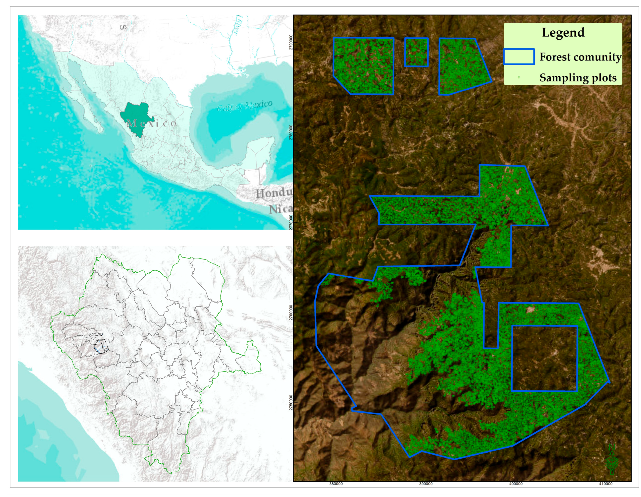
Figure 2.
Scatter plot for h-dbh relationship for full dataset (a) and grouping dataset by cluster (b).
Figure 2.
Scatter plot for h-dbh relationship for full dataset (a) and grouping dataset by cluster (b).
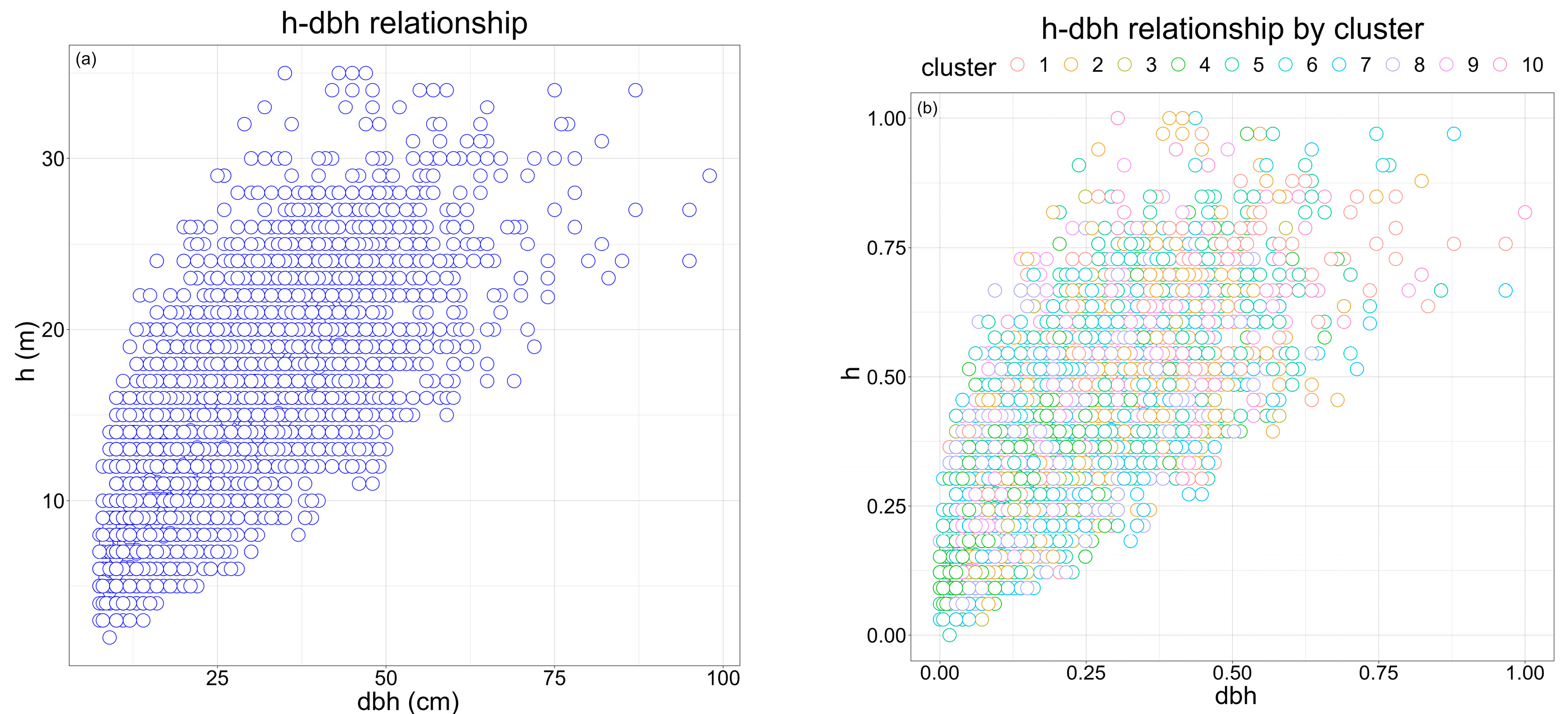
Figure 3.
Plots of ANNs for vectors of c(3, 3, 3) on the left, c(5, 5, 5) on the center, and c(10, 10, 10) on the right, in the hidden layer.
Figure 3.
Plots of ANNs for vectors of c(3, 3, 3) on the left, c(5, 5, 5) on the center, and c(10, 10, 10) on the right, in the hidden layer.
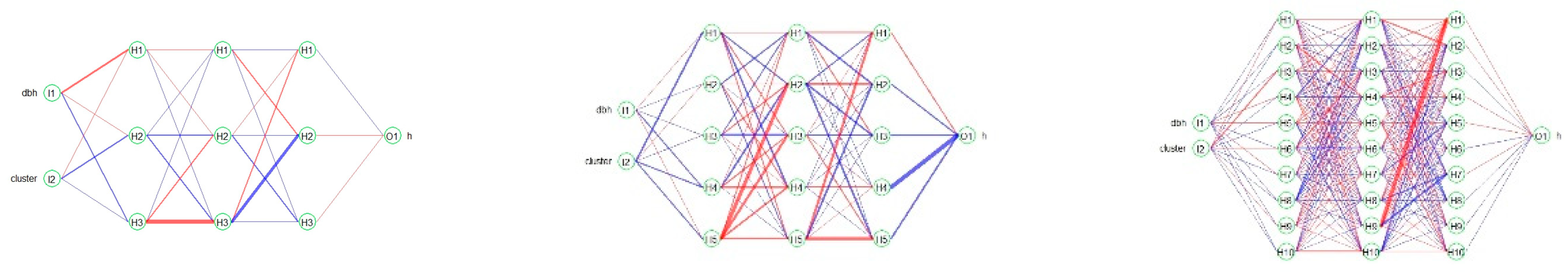
Figure 4.
Plots of RBPANN-tanh (left), RBPANN-softplus (center), and RBPANN-logistic (right) for h-dbh relationship with unsupervised clustering analysis. Bias is included in nodes “B”. Positive weight values in the visual representation are denoted by blue lines, while negative weight values are represented by red lines.

Figure 5.
Residual versus predicted values for RBPANN-tanh model in training phase and each cluster-group.
Figure 5.
Residual versus predicted values for RBPANN-tanh model in training phase and each cluster-group.
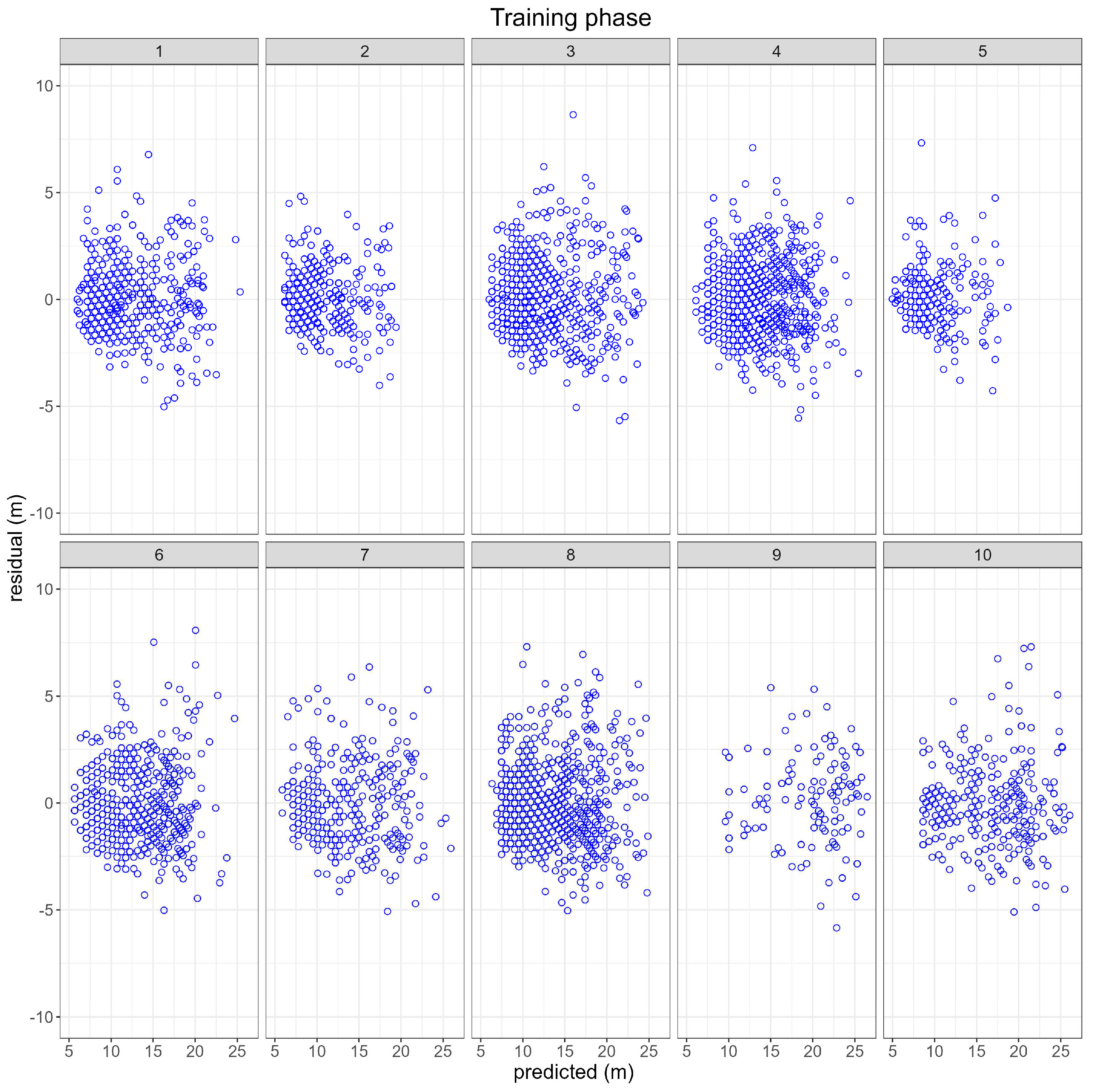
Figure 6.
Residual versus predicted values for RBPANN-tanh model in testing phase for each cluster-group.
Figure 6.
Residual versus predicted values for RBPANN-tanh model in testing phase for each cluster-group.
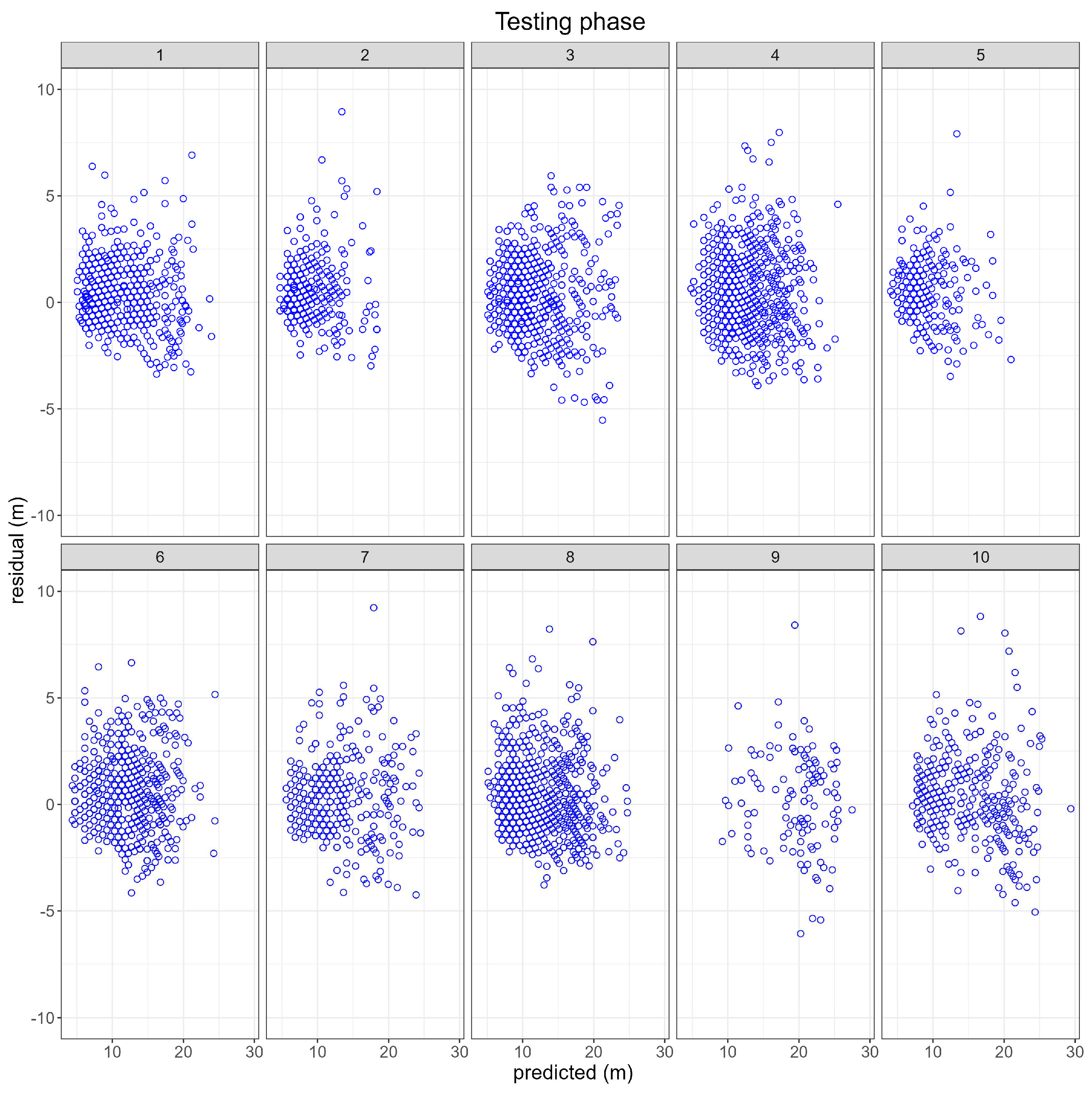

Table 1.
Descriptive statistics for plot-specific variables used in clustering analysis.
| Statistic | |||||
|---|---|---|---|---|---|
| Variable | n | Minimum | Mean | Maximum | SD |
| N | 1000 | 1.0000 | 11.4720 | 57.0000 | 8.7717 |
| BA | 1000 | 0.0007 | 0.0193 | 0.0924 | 0.0137 |
| Dm | 1000 | 8.5000 | 22.9636 | 75.0000 | 7.6788 |
| Hm | 1000 | 4.0000 | 12.8062 | 35.0000 | 3.9813 |
| QMD | 1000 | 8.5147 | 24.7478 | 75.0000 | 8.0708 |
| A | 1000 | 2032.0000 | 2588.2170 | 2978.0000 | 137.3215 |
| S | 1000 | 0.0000 | 43.0499 | 96.0000 | 20.0551 |
| As | 1 | 5 | 9 | 2 | |
N = density (trees per hectare); BA = basal area (m2); Dm = mean diameter (cm); Hm = mean total tree (m); QMD = quadratic mean diameter (cm); A = altitudes (m); S = slope (%); and As = aspect (categorical variable; 1 = Plain, 2 = N, 3 = S, 4 = E, 5 = W, 6 = NE, 7 = SE, 8 = NW, 9 = SW); n = observations; SD = standard deviation.
Table 2.
This is a table. Tables should be placed in the main text near to the first time they are cited.
Table 2.
This is a table. Tables should be placed in the main text near to the first time they are cited.
| Dataset | Statistic | |||||
|---|---|---|---|---|---|---|
| Variable | n | Minimum | Mean | Maximum | SD | |
| Training | h | 5736 | 7.5000 | 21.5362 | 95.0000 | 11.4394 |
| dbh | 5736 | 3.0000 | 12.3900 | 35.0000 | 5.3217 | |
| Testing | h | 5736 | 7.5000 | 21.3846 | 98.0000 | 11.5267 |
| dbh | 5736 | 2.0000 | 12.1742 | 35.0000 | 5.2871 | |
h = total tree height (m); dbh = diameter at breast height (cm); n = observations; SD = standard deviation.
Table 3.
Estimated parameter for h-dbh relationship in Durango pine by NLMEM.
| Parameter | Estimate | SE | DF | t-value | p-value | lower | upper |
|---|---|---|---|---|---|---|---|
| 26.409060 | 1.100113 | 5724 | 24.005770 | <0.00001 | 24.252985 | 28.565134 | |
| 0.029786 | 0.002534 | 5724 | 11.754320 | <0.00001 | 0.024820 | 0.034752 | |
| 1.083133 | 0.040518 | 5724 | 26.732200 | <0.00001 | 1.003723 | 1.162543 | |
| 1.928939 | 0.583997 | 5724 | 3.302992 | 0.000962 | 1.210579 | 3.073574 | |
| 3.110839 | 0.029338 | 5724 | 106.033502 | <0.00001 | 3.054379 | 3.168342 | |
| -3.371745 | 0.106547 | 407 | -31.645570 | <0.00001 | -3.580578 | -3.162913 | |
| -2.840826 | 0.089770 | 320 | -31.645570 | <0.00001 | -3.016775 | -2.664877 | |
| -0.601879 | 0.019019 | 631 | -31.645570 | <0.00001 | -0.639157 | -0.564601 | |
| 3.572580 | 0.112894 | 133 | 31.645570 | <0.00001 | 3.351309 | 3.793851 | |
| 0.773802 | 0.024452 | 925 | 31.645570 | <0.00001 | 0.725876 | 0.821729 | |
| 0.478565 | 0.015123 | 1109 | 31.645570 | <0.00001 | 0.448925 | 0.508206 | |
| 0.945549 | 0.029879 | 364 | 31.645570 | <0.00001 | 0.886985 | 1.004113 | |
| -0.308794 | 0.009758 | 876 | -31.645570 | <0.00001 | -0.327919 | -0.289668 | |
| 0.012327 | 0.000390 | 654 | 31.645570 | <0.00001 | 0.011564 | 0.013091 | |
| 1.340420 | 0.042357 | 317 | 31.645570 | <0.00001 | 1.257400 | 1.423440 |
SE = asymptotic standard error; DF = freedom degrees; sd = standard deviation for random effect between cluster groups; = standard error within-cluster-group.
Table 4.
Fitting statistics for h-dbh relationship in Durango pine by NLMEM.
| Dataset | n | RMSE | SEE | RSEE | FI | E | RE | AIC | BIC | logLik |
| All-dataset | 5736 | 3.1085 | 3.1123 | 25.1193 | 0.6588 | -0.0005 | -0.0042 | 13039.75 | 13139.57 | -13009.75 |
| C1 | 631 | 2.4735 | 2.4889 | 6.4322 | 0.6182 | -0.0324 | -0.3161 | 8834.14 | 772.23 | -736.18 |
| C2 | 407 | 2.5289 | 2.5489 | 6.1485 | 0.5378 | 0.0050 | 0.0515 | 7113.33 | 627.39 | -592.78 |
| C3 | 925 | 2.9631 | 2.9749 | 8.4267 | 0.6525 | -0.1111 | -0.9526 | 16437.91 | 1408.51 | -1369.83 |
| C4 | 1109 | 3.8688 | 3.9442 | 2.9876 | 0.5610 | 0.3416 | 1.7378 | 4306.53 | 388.22 | -358.88 |
| C5 | 320 | 3.1341 | 3.1426 | 10.6971 | 0.6312 | -0.0072 | -0.0610 | 25348.12 | 2153.32 | -2112.34 |
| C6 | 654 | 2.8727 | 2.8792 | 10.3014 | 0.6134 | 0.0555 | 0.4528 | 28074.42 | 2381.60 | -2339.53 |
| C7 | 364 | 3.4345 | 3.4584 | 6.5911 | 0.6329 | -0.0640 | -0.4879 | 10767.05 | 932.64 | -897.25 |
| C8 | 876 | 3.3842 | 3.3939 | 10.2592 | 0.6015 | 0.0210 | 0.1632 | 25618.61 | 2175.54 | -2134.88 |
| C9 | 133 | 3.2098 | 3.2221 | 8.8088 | 0.6138 | -0.0229 | -0.1862 | 18292.63 | 1563.28 | -1524.39 |
| C10 | 317 | 3.6168 | 3.6458 | 5.1452 | 0.6196 | -0.0058 | -0.0353 | 9768.73 | 848.61 | -814.06 |
RMSE = root mean square error (m); SEE = standard error of estimate (m); RSEE = relative SEE (%); FI = fitting index; E = mean error (m); RE = relative (%); AIC = Akaike information criterion; BIC = Bayesian information criterion; logLik = log-likelihood value; C = cluster-group.
Table 5.
Main fitting statistics for RBPANN-tanh, RBPANN-softplus, and RBPANN-logistic activation functions tested for h-dbh relationship.
Table 5.
Main fitting statistics for RBPANN-tanh, RBPANN-softplus, and RBPANN-logistic activation functions tested for h-dbh relationship.
| ANN | Error | Reached Threshold | Steps | AIC | BIC |
| RBPANN-tanh | 27.8455 | 0.0775 | 301 | 577.69 | 2314.52 |
| RBPANN-softplus | 27.3939 | 0.0838 | 1885 | 576.79 | 2313.62 |
| RBPANN-logistic | 28.4113 | 0.0994 | 88 | 578.82 | 2315.65 |
AIC = Akaike information criterion; BIC = Bayesian information criterion.
Table 6.
Fitting statistics for h-dbh relationship in Durango pine by ANNs and different backpropagations activation functions.
Table 6.
Fitting statistics for h-dbh relationship in Durango pine by ANNs and different backpropagations activation functions.
| Dataset | RMSE | SEE | RSEE | FI | E | RE | AIC | BIC | logLik |
|---|---|---|---|---|---|---|---|---|---|
| RBPANN-tanh | |||||||||
| All-dataset | 2.8122 | 2.8134 | 22.7071 | 0.7208 | 0.0001 | -0.0003 | 11872.59 | 11912.52 | -11860.59 |
| C1 | 2.6322 | 2.6427 | 8.0184 | 0.7258 | 0.0002 | 0.0018 | 14644.89 | 1259.09 | -1220.41 |
| C2 | 2.2127 | 2.2264 | 6.1634 | 0.6945 | 0.0073 | 0.0717 | 7745.69 | 681.53 | -645.47 |
| C3 | 2.8170 | 2.8246 | 10.2988 | 0.7020 | -0.0087 | -0.0741 | 22979.70 | 1955.95 | -1914.98 |
| C4 | 2.5795 | 2.5853 | 9.9082 | 0.6883 | 0.0636 | 0.5191 | 25209.16 | 2142.83 | -2100.76 |
| C5 | 2.4178 | 2.4370 | 6.2966 | 0.5776 | -0.6268 | -6.4583 | 6768.31 | 598.64 | -564.03 |
| C6 | 2.8907 | 2.9019 | 8.4977 | 0.6867 | 0.2559 | 2.0805 | 16649.44 | 1426.35 | -1387.45 |
| C7 | 3.1340 | 3.1558 | 6.4423 | 0.6943 | 0.3677 | 2.8037 | 9967.09 | 865.97 | -830.59 |
| C8 | 3.0652 | 3.0740 | 9.9535 | 0.6731 | -0.3691 | -2.8636 | 23537.45 | 2002.11 | -1961.45 |
| C9 | 3.7470 | 3.8200 | 3.0995 | 0.5882 | 1.5107 | 7.6864 | 4204.43 | 379.71 | -350.37 |
| C10 | 3.2490 | 3.2751 | 4.9509 | 0.6930 | -0.1391 | -0.8426 | 8952.96 | 780.63 | -746.08 |
| RBPANN-softplus | |||||||||
| All-dataset | 2.8431 | 2.8443 | 22.9565 | 0.7143 | 0.7146 | -0.0013 | -0.0107 | 11997.88 | 12037.81 |
| C1 | 2.6516 | 2.6621 | 8.0772 | 0.7218 | 0.0489 | 0.4190 | 14755.60 | 1268.32 | -1229.63 |
| C2 | 2.4591 | 2.4744 | 6.8498 | 0.6226 | -0.9459 | -9.2408 | 8777.19 | 767.49 | -731.43 |
| C3 | 2.8529 | 2.8606 | 10.4301 | 0.6944 | 0.4200 | 3.5697 | 23260.85 | 1979.38 | -1938.40 |
| C4 | 2.6003 | 2.6062 | 9.9882 | 0.6833 | 0.3109 | 2.5351 | 25423.15 | 2160.66 | -2118.60 |
| C5 | 2.4956 | 2.5154 | 6.4993 | 0.5499 | -0.9140 | -9.4178 | 7011.62 | 618.91 | -584.30 |
| C6 | 2.8841 | 2.8952 | 8.4781 | 0.6882 | -0.1042 | -0.8472 | 16613.23 | 1423.33 | -1384.44 |
| C7 | 3.1030 | 3.1246 | 6.3787 | 0.7003 | 0.1339 | 1.0213 | 9880.37 | 858.75 | -823.36 |
| C8 | 3.0748 | 3.0837 | 9.9847 | 0.6711 | -0.3712 | -2.8799 | 23603.31 | 2007.59 | -1966.94 |
| C9 | 3.8187 | 3.8931 | 3.1588 | 0.5723 | 1.6461 | 8.3754 | 4264.92 | 384.75 | -355.41 |
| C10 | 3.2550 | 3.2811 | 4.9600 | 0.6919 | 0.0992 | 0.6009 | 8966.90 | 781.80 | -747.24 |
| RBPANN-logistic | |||||||||
| All-dataset | 2.8486 | 2.8498 | 23.0012 | 0.7135 | -0.0052 | -0.0420 | 12020.19 | 12060.12 | -12008.19 |
| C1 | 2.6570 | 2.6676 | 8.0938 | 0.7206 | 0.0785 | 0.6729 | 14786.65 | 1270.90 | -1232.22 |
| C2 | 2.4675 | 2.4828 | 6.8732 | 0.6201 | -0.9254 | -9.0403 | 8810.45 | 770.26 | -734.20 |
| C3 | 2.8586 | 2.8664 | 10.4510 | 0.6932 | 0.4146 | 3.5237 | 23305.34 | 1983.09 | -1942.11 |
| C4 | 2.6024 | 2.6083 | 9.9962 | 0.6827 | 0.2868 | 2.3386 | 25444.48 | 2162.44 | -2120.37 |
| C5 | 2.5183 | 2.5382 | 6.5583 | 0.5417 | -0.9468 | -9.7561 | 7081.01 | 624.69 | -590.08 |
| C6 | 2.9055 | 2.9167 | 8.5411 | 0.6835 | -0.1415 | -1.1503 | 16729.32 | 1433.01 | -1394.11 |
| C7 | 3.0957 | 3.1172 | 6.3636 | 0.7017 | 0.1066 | 0.8129 | 9859.77 | 857.03 | -821.65 |
| C8 | 3.0740 | 3.0828 | 9.9818 | 0.6712 | -0.3751 | -2.9095 | 23597.18 | 2007.08 | -1966.43 |
| C9 | 3.8192 | 3.8936 | 3.1592 | 0.5721 | 1.6756 | 8.5253 | 4265.34 | 384.79 | -355.45 |
| C10 | 3.2584 | 3.2845 | 4.9652 | 0.6912 | 0.1835 | 1.1115 | 8974.85 | 782.46 | -747.90 |
RMSE = root mean square error (m); SEE = standard error of estimate (m); RSEE = relative SEE (%); FI = fitting index; E = mean error (m); RE = relative (%); AIC = Akaike information criterion; BIC = Bayesian information criterion; logLik = log-likelihood value; C = cluster-group.
Table 7.
Ranks and sum of ranks based on the fitting statistics for fitted models in training phase.
Table 7.
Ranks and sum of ranks based on the fitting statistics for fitted models in training phase.
| Model | Dataset | RMSE | SEE | RSEE | FI | E | RE | AIC | BIC | logLik | Rank |
|---|---|---|---|---|---|---|---|---|---|---|---|
| NLMEM | Overall | 4 | 4 | 4 | 4 | 3 | 2 | 4 | 4 | 4 | 33 (4) |
| RBPANN-tanh | Overall | 1 | 1 | 1 | 1 | 4 | 4 | 2 | 1 | 2 | 17 (2) |
| RBPANN-softplus | Overall | 2 | 2 | 2 | 2 | 1 | 3 | 1 | 2 | 1 | 16 (1) |
| RBPANN-logistic | Overall | 3 | 3 | 3 | 3 | 2 | 1 | 3 | 3 | 3 | 24 (3) |
| NLMEM | C1 | 1 | 1 | 1 | 4 | 2 | 2 | 1 | 1 | 1 | 14 |
| RBPANN-tanh | C1 | 2 | 2 | 2 | 1 | 1 | 1 | 2 | 2 | 2 | 15 |
| RBPANN-softplus | C1 | 3 | 3 | 3 | 2 | 3 | 3 | 3 | 3 | 3 | 26 |
| RBPANN-logistic | C1 | 4 | 4 | 4 | 3 | 4 | 4 | 4 | 4 | 4 | 35 |
| NLMEM | C2 | 4 | 4 | 1 | 4 | 1 | 1 | 1 | 1 | 1 | 18 |
| RBPANN-tanh | C2 | 1 | 1 | 2 | 1 | 2 | 2 | 2 | 2 | 2 | 15 |
| RBPANN-softplus | C2 | 2 | 2 | 3 | 2 | 4 | 4 | 3 | 3 | 3 | 26 |
| RBPANN-logistic | C2 | 3 | 3 | 4 | 3 | 3 | 3 | 4 | 4 | 4 | 31 |
| NLMEM | C3 | 4 | 4 | 1 | 4 | 2 | 2 | 1 | 1 | 1 | 20 |
| RBPANN-tanh | C3 | 1 | 1 | 2 | 1 | 1 | 1 | 2 | 2 | 2 | 13 |
| RBPANN-softplus | C3 | 2 | 2 | 3 | 2 | 4 | 4 | 3 | 3 | 3 | 26 |
| RBPANN-logistic | C3 | 3 | 3 | 4 | 3 | 3 | 3 | 4 | 4 | 4 | 31 |
| NLMEM | C4 | 4 | 4 | 1 | 4 | 4 | 2 | 1 | 1 | 1 | 22 |
| RBPANN-tanh | C4 | 1 | 1 | 2 | 1 | 1 | 1 | 2 | 2 | 2 | 13 |
| RBPANN-softplus | C4 | 2 | 2 | 3 | 2 | 3 | 4 | 3 | 3 | 3 | 25 |
| RBPANN-logistic | C4 | 3 | 3 | 4 | 3 | 2 | 3 | 4 | 4 | 4 | 30 |
| NLMEM | C5 | 4 | 4 | 4 | 1 | 1 | 1 | 4 | 4 | 4 | 27 |
| RBPANN-tanh | C5 | 1 | 1 | 1 | 2 | 2 | 2 | 1 | 1 | 1 | 12 |
| RBPANN-softplus | C5 | 2 | 2 | 2 | 3 | 3 | 3 | 2 | 2 | 2 | 21 |
| RBPANN-logistic | C5 | 3 | 3 | 3 | 4 | 4 | 4 | 3 | 3 | 3 | 30 |
| NLMEM | C6 | 1 | 1 | 4 | 4 | 1 | 1 | 4 | 4 | 4 | 24 |
| RBPANN-tanh | C6 | 3 | 3 | 2 | 2 | 4 | 4 | 2 | 2 | 2 | 24 |
| RBPANN-softplus | C6 | 2 | 2 | 1 | 1 | 2 | 2 | 1 | 1 | 1 | 13 |
| RBPANN-logistic | C6 | 4 | 4 | 3 | 3 | 3 | 3 | 3 | 3 | 3 | 29 |
| NLMEM | C7 | 4 | 4 | 4 | 4 | 1 | 1 | 4 | 4 | 4 | 30 |
| RBPANN-tanh | C7 | 3 | 3 | 3 | 3 | 4 | 4 | 3 | 3 | 3 | 29 |
| RBPANN-softplus | C7 | 2 | 2 | 2 | 2 | 3 | 3 | 2 | 2 | 2 | 20 |
| RBPANN-logistic | C7 | 1 | 1 | 1 | 1 | 2 | 2 | 1 | 1 | 1 | 11 |
| NLMEM | C8 | 4 | 4 | 4 | 4 | 1 | 1 | 4 | 4 | 4 | 30 |
| RBPANN-tanh | C8 | 1 | 1 | 1 | 1 | 2 | 2 | 1 | 1 | 1 | 11 |
| RBPANN-softplus | C8 | 3 | 3 | 3 | 3 | 3 | 3 | 3 | 3 | 3 | 27 |
| RBPANN-logistic | C8 | 2 | 2 | 2 | 2 | 4 | 4 | 2 | 2 | 2 | 22 |
| NLMEM | C9 | 1 | 1 | 4 | 1 | 1 | 1 | 4 | 4 | 4 | 21 |
| RBPANN-tanh | C9 | 2 | 2 | 1 | 2 | 2 | 2 | 1 | 1 | 1 | 14 |
| RBPANN-softplus | C9 | 3 | 3 | 2 | 3 | 3 | 3 | 2 | 2 | 2 | 23 |
| RBPANN-logistic | C9 | 4 | 4 | 3 | 4 | 4 | 4 | 3 | 3 | 3 | 32 |
| NLMEM | C10 | 4 | 4 | 4 | 4 | 1 | 1 | 4 | 4 | 4 | 30 |
| RBPANN-tanh | C10 | 1 | 1 | 1 | 1 | 3 | 3 | 1 | 1 | 1 | 13 |
| RBPANN-softplus | C10 | 2 | 2 | 2 | 2 | 2 | 2 | 2 | 2 | 2 | 18 |
| RBPANN-logistic | C10 | 3 | 3 | 3 | 3 | 4 | 4 | 3 | 3 | 3 | 29 |
RMSE = root mean square error; SEE = standard error of estimate; RSEE = relative SEE; FI = fitting index; E = mean error; RE = relative E; AIC = Akaike information criterion; BIC = Bayesian information criterion; logLik = log-likelihood value; C = cluster-group.
Table 8.
Testing statistics for h-dbh relationship in Durango pine by NLMEM in testing phase.
| Dataset | n | RMSE | SEE | RSEE | FI | E | RE | AIC | BIC | logLik |
|---|---|---|---|---|---|---|---|---|---|---|
| All-dataset | 5736 | 3.1438 | 3.1476 | 25.8549 | 0.6464 | -0.1611 | -1.3229 | 13169.29 | 13269.10 | -13139.29 |
| C1 | 631 | 2.7037 | 2.7141 | 24.1931 | 0.6893 | -0.0987 | -0.8795 | 15671.32 | 1344.87 | -1305.94 |
| C2 | 407 | 2.9045 | 2.9228 | 29.6973 | 0.4680 | 1.2223 | 12.4194 | 10249.76 | 890.11 | -854.15 |
| C3 | 925 | 3.0941 | 3.1029 | 27.5443 | 0.6136 | -0.7206 | -6.3964 | 23870.14 | 2029.86 | -1989.18 |
| C4 | 1109 | 3.0509 | 3.0578 | 25.0690 | 0.6102 | -0.0942 | -0.7725 | 29971.18 | 2539.72 | -2497.60 |
| C5 | 320 | 2.7563 | 2.7797 | 28.6992 | 0.5175 | 0.9194 | 9.4926 | 7263.59 | 639.50 | -605.30 |
| C6 | 654 | 3.1718 | 3.1834 | 25.4080 | 0.6085 | 0.1428 | 1.1398 | 19047.71 | 1626.51 | -1587.31 |
| C7 | 364 | 3.4512 | 3.4752 | 26.2781 | 0.6545 | -0.7996 | -6.0462 | 10839.28 | 938.67 | -903.27 |
| C8 | 876 | 3.0615 | 3.0704 | 24.6303 | 0.6290 | -0.1456 | -1.1680 | 23216.40 | 1975.28 | -1934.70 |
| C9 | 133 | 5.0061 | 5.1138 | 25.4219 | 0.2128 | -2.4332 | -12.0959 | 4665.31 | 417.55 | -388.78 |
| C10 | 317 | 3.8668 | 3.8957 | 24.6024 | 0.5555 | -0.7956 | -5.0245 | 10991.37 | 950.90 | -915.95 |
RMSE = root mean square error (m); SEE = standard error of estimate (m); RSEE = relative SEE (m); FI = fitting index; E = mean error (m); RE = relative E (%); AIC = Akaike information criterion; BIC = Bayesian information criterion; logLik = log-likelihood value; C = cluster-group.
Table 9.
Testing statistics for both overall dataset and each cluster-group in testing phase with ANNs approaches.
Table 9.
Testing statistics for both overall dataset and each cluster-group in testing phase with ANNs approaches.
| Dataset | RMSE | SEE | RSEE | FI | E | RE | AIC | BIC | logLik |
|---|---|---|---|---|---|---|---|---|---|
| RBPANN-tanh | |||||||||
| All-dataset | 2.8693 | 2.8706 | 23.5793 | 0.7055 | 0.6603 | 5.4241 | 12103.39 | 12143.32 | -12091.39 |
| C1 | 2.5090 | 2.5186 | 8.1057 | 0.7324 | 0.6015 | 5.3617 | 14492.43 | 1246.63 | -1207.70 |
| C2 | 2.4793 | 2.4949 | 7.1292 | 0.6124 | 0.8309 | 8.4421 | 8726.27 | 763.15 | -727.19 |
| C3 | 2.7294 | 2.7372 | 10.1704 | 0.6994 | 0.4046 | 3.5917 | 21218.12 | 1808.86 | -1768.18 |
| C4 | 2.8842 | 2.8907 | 11.1931 | 0.6516 | 0.8969 | 7.3531 | 28460.68 | 2413.85 | -2371.72 |
| C5 | 2.3880 | 2.4083 | 6.0227 | 0.6378 | 0.0825 | 0.8517 | 6234.38 | 553.73 | -519.53 |
| C6 | 3.0888 | 3.1001 | 9.1436 | 0.6287 | 1.2080 | 9.6415 | 18609.70 | 1590.01 | -1550.81 |
| C7 | 3.1665 | 3.1885 | 6.4643 | 0.7091 | 0.8613 | 6.5128 | 10085.03 | 875.82 | -840.42 |
| C8 | 2.7710 | 2.7790 | 9.2458 | 0.6961 | 0.1519 | 1.2183 | 21146.63 | 1802.80 | -1762.22 |
| C9 | 4.2322 | 4.3232 | 3.2613 | 0.4374 | 1.8156 | 9.0259 | 4177.60 | 376.91 | -348.13 |
| C10 | 3.4732 | 3.4992 | 5.7063 | 0.6414 | 0.5225 | 3.2997 | 10118.01 | 878.12 | -843.17 |
| RBPANN-softplus | |||||||||
| All-dataset | 2.8764 | 2.8776 | 23.6371 | 0.7040 | 0.6578 | 5.4029 | 12131.48 | 12171.41 | -12119.48 |
| C1 | 2.5181 | 2.5278 | 8.1353 | 0.7305 | 0.6756 | 6.0219 | 14550.00 | 1251.43 | -1212.50 |
| C2 | 2.3388 | 2.3536 | 6.7253 | 0.6551 | -0.0814 | -0.8266 | 8164.99 | 716.38 | -680.42 |
| C3 | 2.8312 | 2.8393 | 10.5500 | 0.6765 | 0.8131 | 7.2176 | 21992.85 | 1873.42 | -1832.74 |
| C4 | 2.9657 | 2.9724 | 11.5095 | 0.6317 | 1.1148 | 9.1400 | 29209.97 | 2476.29 | -2434.16 |
| C5 | 2.4000 | 2.4204 | 6.0529 | 0.6342 | -0.2679 | -2.7660 | 6270.23 | 556.72 | -522.52 |
| C6 | 2.9772 | 2.9881 | 8.8135 | 0.6550 | 0.7866 | 6.2785 | 18002.41 | 1539.40 | -1500.20 |
| C7 | 3.1029 | 3.1244 | 6.3344 | 0.7207 | 0.6147 | 4.6485 | 9907.23 | 861.00 | -825.60 |
| C8 | 2.7748 | 2.7828 | 9.2584 | 0.6952 | 0.1450 | 1.1632 | 21174.89 | 1805.15 | -1764.57 |
| C9 | 4.3045 | 4.3971 | 3.3171 | 0.4180 | 2.0025 | 9.9547 | 4226.81 | 381.01 | -352.23 |
| C10 | 3.5266 | 3.5530 | 5.7940 | 0.6303 | 0.8555 | 5.4026 | 10242.05 | 888.46 | -853.50 |
| RBPANN-logistic | |||||||||
| All-dataset | 2.8820 | 2.8832 | 23.6832 | 0.7029 | 0.6484 | 5.3263 | 12153.85 | 12193.77 | -12141.85 |
| C1 | 2.5071 | 2.5168 | 8.0998 | 0.7328 | 0.6480 | 5.7760 | 14481.07 | 1245.68 | -1206.76 |
| C2 | 2.3476 | 2.3624 | 6.7505 | 0.6525 | -0.0800 | -0.8123 | 8200.94 | 719.38 | -683.41 |
| C3 | 2.8287 | 2.8368 | 10.5405 | 0.6771 | 0.8418 | 7.4726 | 21973.90 | 1871.84 | -1831.16 |
| C4 | 2.9718 | 2.9785 | 11.5331 | 0.6302 | 1.1385 | 9.3342 | 29264.97 | 2480.87 | -2438.75 |
| C5 | 2.3833 | 2.4035 | 6.0108 | 0.6392 | -0.2199 | -2.2702 | 6220.20 | 552.55 | -518.35 |
| C6 | 2.9674 | 2.9783 | 8.7844 | 0.6573 | 0.8301 | 6.6255 | 17947.97 | 1534.87 | -1495.66 |
| C7 | 3.1024 | 3.1240 | 6.3335 | 0.7208 | 0.6342 | 4.7956 | 9905.96 | 860.90 | -825.50 |
| C8 | 2.7763 | 2.7843 | 9.2634 | 0.6949 | 0.1438 | 1.1539 | 21186.18 | 1806.09 | -1765.51 |
| C9 | 4.2538 | 4.3453 | 3.2780 | 0.4316 | 1.9452 | 9.6698 | 4192.42 | 378.14 | -349.37 |
| C10 | 3.4913 | 3.5174 | 5.7360 | 0.6377 | 0.7841 | 4.9519 | 10160.28 | 881.65 | -846.69 |
RMSE = root mean square error (m); SEE = standard error of estimate (m); RSEE = relative SEE (%); FI = fitting index; E = mean error (m); RE = relative E (%); AIC = Akaike information criterion; BIC = Bayesian information criterion; logLik = log-likelihood value; C = cluster-group.
Table 10.
Ranks and sum of ranks based on the fitting statistics for fitted models in testing phase.
Table 10.
Ranks and sum of ranks based on the fitting statistics for fitted models in testing phase.
| Model | Dataset | RMSE | SEE | RSEE | FI | E | RE | AIC | BIC | logLik | Rank |
|---|---|---|---|---|---|---|---|---|---|---|---|
| NLMEM | Overall | 4 | 4 | 4 | 4 | 4 | 4 | 4 | 4 | 4 | 36 (4) |
| RBPANN-tanh | Overall | 1 | 1 | 1 | 1 | 1 | 1 | 1 | 1 | 1 | 9 (1) |
| RBPANN-softplus | Overall | 2 | 2 | 2 | 2 | 2 | 2 | 2 | 2 | 2 | 18 (2) |
| RBPANN-logistic | Overall | 3 | 3 | 3 | 3 | 3 | 3 | 3 | 3 | 3 | 27 (3) |
| NLMEM | C1 | 4 | 4 | 4 | 4 | 1 | 1 | 4 | 4 | 4 | 30 |
| RBPANN-tanh | C1 | 2 | 2 | 2 | 2 | 2 | 2 | 2 | 2 | 2 | 18 |
| RBPANN-softplus | C1 | 3 | 3 | 3 | 3 | 4 | 4 | 3 | 3 | 3 | 29 |
| RBPANN-logistic | C1 | 1 | 1 | 1 | 1 | 3 | 3 | 1 | 1 | 1 | 13 |
| NLMEM | C2 | 4 | 4 | 4 | 4 | 4 | 4 | 4 | 4 | 4 | 36 |
| RBPANN-tanh | C2 | 3 | 3 | 3 | 3 | 3 | 3 | 3 | 3 | 3 | 27 |
| RBPANN-softplus | C2 | 1 | 1 | 1 | 1 | 2 | 2 | 1 | 1 | 1 | 11 |
| RBPANN-logistic | C2 | 2 | 2 | 2 | 2 | 1 | 1 | 2 | 2 | 2 | 16 |
| NLMEM | C3 | 4 | 4 | 4 | 4 | 2 | 2 | 4 | 4 | 4 | 32 |
| RBPANN-tanh | C3 | 1 | 1 | 1 | 1 | 1 | 1 | 1 | 1 | 1 | 9 |
| RBPANN-softplus | C3 | 3 | 3 | 3 | 3 | 3 | 3 | 3 | 3 | 3 | 27 |
| RBPANN-logistic | C3 | 2 | 2 | 2 | 2 | 4 | 4 | 2 | 2 | 2 | 22 |
| NLMEM | C4 | 4 | 4 | 4 | 4 | 1 | 1 | 4 | 4 | 4 | 30 |
| RBPANN-tanh | C4 | 1 | 1 | 1 | 1 | 2 | 2 | 1 | 1 | 1 | 11 |
| RBPANN-softplus | C4 | 2 | 2 | 2 | 2 | 3 | 3 | 2 | 2 | 2 | 20 |
| RBPANN-logistic | C4 | 3 | 3 | 3 | 3 | 4 | 4 | 3 | 3 | 3 | 29 |
| NLMEM | C5 | 4 | 4 | 4 | 4 | 4 | 4 | 4 | 4 | 4 | 36 |
| RBPANN-tanh | C5 | 2 | 2 | 2 | 2 | 1 | 1 | 2 | 2 | 2 | 16 |
| RBPANN-softplus | C5 | 3 | 3 | 3 | 3 | 3 | 3 | 3 | 3 | 3 | 27 |
| RBPANN-logistic | C5 | 1 | 1 | 1 | 1 | 2 | 2 | 1 | 1 | 1 | 11 |
| NLMEM | C6 | 4 | 4 | 4 | 4 | 1 | 1 | 4 | 4 | 4 | 30 |
| RBPANN-tanh | C6 | 3 | 3 | 3 | 3 | 4 | 4 | 3 | 3 | 3 | 29 |
| RBPANN-softplus | C6 | 2 | 2 | 2 | 2 | 2 | 2 | 2 | 2 | 2 | 18 |
| RBPANN-logistic | C6 | 1 | 1 | 1 | 1 | 3 | 3 | 1 | 1 | 1 | 13 |
| NLMEM | C7 | 4 | 4 | 4 | 4 | 3 | 3 | 4 | 4 | 4 | 34 |
| RBPANN-tanh | C7 | 3 | 3 | 3 | 3 | 4 | 4 | 3 | 3 | 3 | 29 |
| RBPANN-softplus | C7 | 2 | 2 | 2 | 2 | 1 | 1 | 2 | 2 | 2 | 16 |
| RBPANN-logistic | C7 | 1 | 1 | 1 | 1 | 2 | 2 | 1 | 1 | 1 | 11 |
| NLMEM | C8 | 4 | 4 | 4 | 4 | 3 | 3 | 4 | 4 | 4 | 34 |
| RBPANN-tanh | C8 | 1 | 1 | 1 | 1 | 4 | 4 | 1 | 1 | 1 | 15 |
| RBPANN-softplus | C8 | 2 | 2 | 2 | 2 | 2 | 2 | 2 | 2 | 2 | 18 |
| RBPANN-logistic | C8 | 3 | 3 | 3 | 3 | 1 | 1 | 3 | 3 | 3 | 23 |
| NLMEM | C9 | 4 | 4 | 4 | 4 | 4 | 4 | 4 | 4 | 4 | 36 |
| RBPANN-tanh | C9 | 1 | 1 | 1 | 1 | 1 | 1 | 1 | 1 | 1 | 9 |
| RBPANN-softplus | C9 | 3 | 3 | 3 | 3 | 3 | 3 | 3 | 3 | 3 | 27 |
| RBPANN-logistic | C9 | 2 | 2 | 2 | 2 | 2 | 2 | 2 | 2 | 2 | 18 |
| NLMEM | C10 | 4 | 4 | 4 | 4 | 3 | 3 | 4 | 4 | 4 | 34 |
| RBPANN-tanh | C10 | 1 | 1 | 1 | 1 | 1 | 1 | 1 | 1 | 1 | 9 |
| RBPANN-softplus | C10 | 3 | 3 | 3 | 3 | 4 | 4 | 3 | 3 | 3 | 29 |
| RBPANN-logistic | C10 | 3 | 3 | 3 | 3 | 4 | 4 | 3 | 3 | 3 | 29 |
RMSE = root mean square error (m); SEE = standard error of estimate; RSEE = relative SEE; FI = fitting index; E = mean error; RE = relative E; AIC = Akaike information criterion; BIC = Bayesian information criterion; logLik = log-likelihood value; C = cluster-group.
Disclaimer/Publisher’s Note: The statements, opinions and data contained in all publications are solely those of the individual author(s) and contributor(s) and not of MDPI and/or the editor(s). MDPI and/or the editor(s) disclaim responsibility for any injury to people or property resulting from any ideas, methods, instructions or products referred to in the content. |
© 2023 by the authors. Licensee MDPI, Basel, Switzerland. This article is an open access article distributed under the terms and conditions of the Creative Commons Attribution (CC BY) license (http://creativecommons.org/licenses/by/4.0/).
Copyright: This open access article is published under a Creative Commons CC BY 4.0 license, which permit the free download, distribution, and reuse, provided that the author and preprint are cited in any reuse.


