
Submitted:
06 July 2023
Posted:
07 July 2023
You are already at the latest version
Abstract
(1) Background: Stereological estimations significantly contributed to our anatomical and physiological understanding of the lung by providing an average distribution of measured parameters over the entire lung parenchyma. However, most structural lung diseases show a very inhomogeneous pattern of alterations. (2) Methods: We developed a novel protocol for the analysis of all pulmonary airspaces. Our pipeline starts with high-resolution synchrotron radiation-based X-ray tomographic microscopy (SRXTM) and consists of (i) image segmentation with the combination of the free machine-learning tool Ilastik and ImageJ and (ii) calculation of the airspace diameter distribution of an entire lung using a diameter map function. To evaluate the new pipeline, lungs from adult mice with cystic fibrosis (CF)-like lung disease (ENaC-transgenic mice) or mice with elastase-induced emphysema were compared to healthy controls. (3) Results: We were able to show the distribution of airspace diameters throughout the entire lung, as well as separately for the conducting airways and the gas-exchange area. In the pathobiological context, we observed an irregular widening of parenchymal airspaces in mice with CF-like lung disease and elastase-induced emphysema. Comparable results were obtained when analyzing lungs imaged with μCT, suggesting that our pipeline is applicable to different kinds of imaging modalities. (4) Conclusions: We conclude that the airspace diameter map is well suited for a detailed analysis of unevenly distributed structural alterations in chronic muco-obstructive lung diseases such as cystic fibrosis and COPD.
Keywords:
lung disease
; cystic fibrosis
; pulmonary emphysema
; image analysis
; artificial intelligence
; X-ray tomographic microscopy
; micro-computed X-ray tomography / micro-CT
; stereology.
1. Introduction
The lung function is readily assessed with pulmonary function tests, which include spirometry, lung volume measurements and diffusion capacity for carbon monoxide allowing for discrimination between the healthy and the lung affected by obstructive and restrictive damage [1]. These strategies, while very useful for the initial diagnosis, do not permit to localize the damage within the lung. Hence, they are often complemented by X-ray computed tomography (CT) or magnetic resonance imaging (MRI), the two main lung-imaging techniques [2,3]. Both techniques have been used in the clinics for more than 50 years, each with specific sets of pros and cons. While MRI provides a good soft tissue contrast without the risk of ionizing radiation, the image resolution is much lower when compared to the CT, especially for the lung parenchyma [4]. Recently, the dark-field x-ray imaging has been suggested as a complement to the CT and applied on animals and human patients with pulmonary pathologies [5,6,7,8]. A technique requires 100 times lower doses than the regular thorax CT and distinguishes well different stages of lung emphysema and pulmonary fibrosis.
To look at the lung microstructure, micro-X-ray computed tomography (µCT) with improved pixel size down to 100 nanometers, is commonly used for both animal and human studies [9,10]. A version of µCT with the highest resolution and image quality available is synchrotron radiation X-ray tomographic microscopy (SRXTM). This technique has the advantage of being operated with a monochromatic, high flux, partially coherent, and nearly parallel beam instead of the cone beam of a classical µCT [11]. Furthermore, the vast volume of data produced requires high computational power and skills as well as large storage capacity. Because of these drawbacks, the analysis of lung microstructure has been limited and often only applied to one or a few regions of the lung [12,13,14].
The extensive advance in the field of lung imaging techniques is narrowly followed by the development in the field of image analysis. Stereology has been the principal approach in lung image analysis and is crucial in addressing the structure of the homogeneous healthy lung. In fact, due to this approach we have a broad knowledge on both bronchial tree and gas-exchange area of the lung of many different species [15]. Stereology, however, has one main limitation. The analysis is not done on the entire lung, but rather on systematic random selected lung slices, and the results are then extrapolated to the entire lung. Because healthy lung parenchyma is isotropic and homogeneous, a small sample is sufficient to give accurate results, if it is properly sampled. Since in many lung diseases, the distribution of the damage is often heterogeneous, a stereological approach becomes much more time consuming, because the fraction of the lung which has to be analyzed increases dramatically up to the entire lung. For muco-obstructive lung diseases such as cystic fibrosis (CF) and COPD, as well as interstitial lung diseases such as pulmonary fibrosis, the only way to properly address the extent of the damage is by analyzing the entire lung [16,17,18,19,20,21]. While many automated and semi-automated approaches for an analysis of the entire lung have been suggested in the recent decade [22,23], no complete analysis of lung airspace distribution of the total murine lung is available to date.
In line with this, we propose a novel pipeline for analysis of images obtained with SRXTM and µCT, which allows for an in-depth study of airspace distributions in the entire mouse and rat lung. Furthermore, the pipeline can be used to extract and separately analyze any of the lung compartments. To validate our pipeline, we analyzed SRXTM images of two different lung disease models: (i) βENaC-transgenic mice, which develop a cystic fibrosis-like lung disease (CF) [24,25,26], and (ii) elastase-induced emphysema. In both cases, we compared diseased to healthy mouse lungs. We observed a clear shift towards larger size airspaces in both lung diseases as well as a completely different pattern in enlarged airspace distribution between the CF and elastase-induced emphysema. Furthermore, comparable results for the same lungs were obtained even for images with lower signal to noise ratio acquired by classical µCT, suggesting that our pipeline is applicable to commonly used and more readily accessible imaging techniques.
2. Materials and Methods
2.1. Mice
Animals were kept in specific pathogen-free facilities exposed to 12h day/12h night cycles with food and drinking water ad libitum. The breading, treatment protocol (where applicable) and sacrificing of the animals was approved by the IACUC of the University of Heidelberg, Germany, for the βENaC-Tg mice and the Institutional Ethics Committee on Animal Care of the University of Geneva, Switzerland and in accordance with the Veterinary Office of the Canton of Geneva for the C57BL/6J mice.
The C57BL/6J mice used for elastase/saline instillation were randomly allocated (by a coin toss), at 11 weeks of age, to either vehicle or elastase receiving group, with the prerequisite that each group contains comparable numbers of female and male mice. Elastase was administered intranasally as described previously [27]. Briefly, mice were anesthetized with 0.1 mg/kg body weight buprenorphine (Temgesic, Indivior Schweiz AG, CH) for 1 hour and subsequently instilled intranasal under 5% isoflurane anesthesia with vehicle or elastase (concentration of 0.2 U/g body weight; High purity porcine pancreatic elastase, #EC134, Elastin Products, Owensville, MO, USA). The βENaC-Tg and the corresponding wild-type control (ctrl) mice were sacrificed at post-natal day 36 (pnd36) by a ketamine and xylazine overdose. The elastase/saline instilled mice were sacrificed on post-elastase day (ped) 21. Immediately after the mice (βENaC-Tg [24] and elastase treated mice, as well as all controls) were sacrificed, the thorax was opened, and the collapsed lungs were filled with freshly prepared 4% paraformaldehyde in phosphate buffered saline (PBS) via the trachea at a pressure of 20 cm water column [28,29]. Afterwards the tracheas were ligated, the lungs were removed, fixed in fresh fixative (4% paraformaldehyde) for 24 h, washed into 70% ethanol and shipped from the University of Heidelberg (βENaC-Tg mice) or the University of Geneva (C57BL/6J mice) to the University of Bern.
Upon receiving the lungs, the tissue was post-fixed in freshly prepared fixative. The volume of the lungs was determined by water displacement [30]. Afterwards, the fixative was removed with PBS and the lungs were washed stepwise into 100% ethanol and critical point dried using a Leica EM CPD 300 device (Leica Microsystems GmbH, Wetzlar Germany) [31,32]. Samples were placed in a 500 μm Eppendorf tube and secured with a piece of cleansing tissue. The tubes were glued upside down on a standard scanning electron microscopy sample holder (PLANO GmbH, Wetzlar, Germany).
2.2. Imaging and reconstruction of the lung samples
2.2.1. Imaging by high-resolution synchrotron radiation-based X-ray tomographic microscopy (SRXTM) at the TOMCAT beamline
The TOMCAT beamline (TOmographic Microscopy and Coherent rAdiology experimenTs, X02DA) at the Swiss Light Source (Paul Scherrer Institute, Villigen, Switzerland) was used for image acquisition with a monochromatic X-ray beam at an energy of 12 keV. To record the images, we used a high numerical aperture white-beam compatible 4x macroscope (Optique Peter, Lentilly, France) equipped with a PCO.Edge 5.5 sCMOS camera (PCO GmbH, Kehlheim, Germany) and a 17 µm thick LSO:Tb (E17LSb) scintillator (Crytur, Turnov, Czech Republic), yielding a pixel size of 1.625 x 1.625 µm2 and a field of view of 4.2 x 3.5 mm2. The sample was placed at the distance of 50 cm from the detector and imaged using a protocol of stacked 360° scans (a stack of 4-7 scans in parallel to the rotational axis and an extended field of view by a factor of ca. 1.9 perpendicularly to the rotational axis). The total scan time was 21-42 min/lung for the 36 days old mice (βENaC-Tg and the controls) and 41-48 min/lung for the 100 days old mice (elastase-instilled and the ctrl’s). The number of projections was set to 3001/per 360° scan at an exposure time of 100 ms [33,34].
The reconstructions of individual 3D-datasets were performed as described previously in detail in [34]. In brief, we first applied dark-field correction using the mean of 30 calibration dark frames, followed by a dynamic flat-field correction [35]. To increase the air-tissue contrast, the projections were submitted to a phase retrieval process using a method developed by Paganin et al [36] with δ and β parameters set to 2e-07 and 2.8e-10 and the propagation distance of 50 mm. Subsequently, the projections were reconstructed using the gridrec algorithm with recorded angular positions and center offsets [37,38]. The rotation center of individual samples was determined manually by screening multiple rotation axis positions.
2.2.2. μCT scans
A large-capacity 3D X-ray microscope (Bruker SkyScan 1272 (Control software version 1.1.19, Bruker microCT, Kontich, Belgium)), equipped with a Hamamatsu L11871_20 X-ray source and a XIMEA xiRAY16 camera, was used to image the left lobes of one ctrl and two elastase-instilled lungs. The X-ray source was set to a tube voltage of 50.0 kV and a tube current of 200.0 µA, the X-ray spectrum was not filtered. We recorded a set of three stacked scans overlapping the total height of each sample. Two samples (one control (ctrl) and one emphysema (El-1)) were recorded with a camera size of 4904 x 3280 pixels, a frame averaging 3, and an exposure time of 1331 ms per projection. The large lateral extent of the third emphysema sample (El-2) necessitated recording it with so-called stitched projections, with a (virtual) camera size of 9328 x 3277 pixels. This sample was recorded with an exposure time of 800 ms per projection. All samples were scanned with approx. 1900 projections at every 0.1° step over a 180° sample rotation. The total scan duration was about 3 h and 50 min per stack for the ctrl and E1 sample, and 5h and 39m for the E2 sample. This resulted in a total scanning time of approximately 40 h. The projection images were then subsequently reconstructed into a 3D stack of images with NRecon (Version 1.7.4.2, Bruker microCT, Kontich Belgium) using a ring artifact correction of 14, yielding 8-bit files with an isometric voxel size of 1.5 µm.
2.3. Image stitching and analysis
2.3.1. Stitching of individual SRXTM scans
The individual data volumes (from 4 to 7 blocks) were assembled into one z-stack with the non-rigid stitching framework NRStitcher [39]. The final stitched datasets size for the βENaC-Tg lungs and the day36 controls were in the range between 231 and 805 GB with width x length x height dimensions of 4100-5700 x 4300-6396 x 6070-10740 voxels, which corresponds to a physical volume of 6.7-9.3 x 7.0-10.4 x 9.9-17.5 mm3. The final stitched datasets size for the elastase/saline-instilled lungs was a 16-bit image in the range between 401 and 609 GB with dimensions of 4100-5000 x 4100-4600 x 11837-14230 voxels, corresponding to a physical volume of 6.7-8.1 x 6.7-7.5 x 19.2-23.1 mm3. The illustration of the output of image reconstruction and stitching is shown in Figure 1B,C.
2.3.2. Statistical analysis of the results
In order to compare the histograms of βENaC-Tg/elastase-instilled- and control-samples the following parameters were compared: [i] peak position and height (Figure 2A), [ii] at half peak height the peak width and the position of the left and right shoulders (Figure 2B), and [iii] the area under the curve left and right of the crossing point of the two plots (e.g. βENaC-Tg and control, as well as elastase-instilled and control) (Figure 2C,D). Because no data point was located exactly at the half peak height, the two closed data points and linear interpolation were used. The surface under the curve is a direct measure of the airspace volumes and can be converted to the airspace volume by the following formula: (surface under the curve multiplied by voxel size (=1.625^3))/shrinkage factor.
The student’s t-test, two-tailed and homoscedastic, was performed to determine the significance of the difference between the ctrl and diseased lungs of the above-mentioned parameters.
2.3.3. Plotting and visualization of the distribution of enlarged airspaces
The results were plotted with the R project and ggplot2 package and the data were fitted with the generalized additive model (GAM) with integrated smoothness estimation with the following formula y ~ s (x, k = 50) (mgcv package), with k representing the degrees of freedom [40,41,42,43]. For visual illustration, we used Imaris software (version 9.3.1, Bitplane, Zürich, Switzerland). To account for the increased lung volume in mice with CF and emphysema, we presented the raw counts together with normalized probability curves.
3. Results
3.1. Segmentations
3.1.1. Segmentation of pulmonary tissue
Samples were imaged in 3D by SRXTM (see above, 2.2.1) and/or with high-resolution µCT (see above, 2.2.2). Reconstructed images were further processed with an open-source machine-learning tool Ilastik (version 1.3.3) [44]. This approach was chosen due to the high level of background gradient detected in the samples. We used a pixel classification workflow that contains generic pixel features including pixel intensity, edge filters and texture description selectable on different scales that are defined by a sigma factor. Furthermore, all the features can be computed either in 2D or in 3D. In our study, we used intensity features with the sigma values of 0.3 and 1 in 3D and 3.5 and 10 in 2D, edge filters with the sigma values of 0.7 and 1.6 in 3D and 5 in 2D, texture features with the sigma values of 1 in 3D and 3.5 and 10 in 2D. The Ilastik projects were trained on 12 consecutive slices at 3 different positions in the z stack to best represent all the different background gradients within the z-stack. Following the features selection process, a manual input was given in order to label the lung tissue and separate it from the rest of the image (lung airspaces and the background surrounding the lung). Due to the large amount of data, the object classification by Ilastik was done in “headless” mode, which processes the images by dividing them in independent blocks. For the images obtained by SRXTM, each of the samples in the βENaC-Tg group was segmented with a different Ilastik project and for the samples in the emphysema group we used only 2 projects for segmentation of the controls and only 1 project for segmentation of all the elastase-instilled samples. For the images obtained with the µCT, each of the 3 samples were segmented with a different project. The illustration of the ilastik segmentation output is shown in (Figure 1D).
3.1.2. Segmentation of pulmonary airspaces
To obtain a segmentation of the pulmonary airspaces, we first created the mask of all lung lobes (tissues and airspaces). First, a tissue “dilation” was applied to the segmentation of the pulmonary tissue. A radius of five pixels was used to close small holes in the alveolar septa. Second, the “fill holes” function of ImageJ was applied to the “dilated” dataset [45]. Third, the obtained mask of the lung lobes, was eroded by the same radius as applied in the first step (dilation).
The final segmentation of pulmonary airspaces was created by multiplying the inverted result of segmentation of the pulmonary tissue with the mask of lung lobes. The output of the segmentation process is a binary image with the same dimensions as the input image obtained after the stitching step. For the analysis of the µCT images, the final segmentation file was further processed with the “analyze particles” function of ImageJ by applying a filter size of 50 pixel2, meaning that all the particles whose area is smaller than 50 pixel2 (e.g in the case of a perfect circle, all the particles with the radius smaller than 4 pixels) will be removed. This “cleaning” step was required because of the higher background level in the images obtained with the µCT. An illustration of the final segmentation is shown in Figure 1E.
3.2. Calculation of airspace diameter distribution using the thickness map algorithm
The calculations of airspace diameter distribution were performed as described previously [46]. Briefly, spheres of maximal diameter were fitted into the 3-dimensional lung airspaces using the “thickness map” function of the software Pi2 (https://github.com/arttumiettinen/pi2) (Figure 3).
The airways diameters were extracted and mapped as grey values of every voxel. An illustration of the airway diameter map is shown in Figure 1F. Using the ImageJ function “Histogram” with the 150 bins of a bin size of 2 and x value range from 3 to 303, a histogram distribution was calculated showing the number of voxels of the certain grey value or the airway diameter, respectively.
To normalize for the uneven volume between individual lungs we converted voxel counts into voxel probability by dividing the count per determined diameter by the total voxel count of the lung. Finally, to account for the tissue shrinkage due to critical point drying, we compared lung volume obtained by water displacement with the volume obtained from the mask of all lung lobes (described in the previous chapter). We observed an average shrinkage of the sample volume of 70.6% (+/- 1.2%). This resulted in a mean volume of 29.4% (shrinkage factor) of the original volume. These values were not far from the values published for the rat lung shrinkage where the shrinking factor was estimated to 36.8% [47]. We corrected all our measurements for shrinkage.
3.3. Extraction of the conducting airways
The bronchial tree of the lungs is divided into two parts. The conducting and the gas-exchanging airways. The conducting airways consist of the bronchi (larger conducting airways, containing cartilage in their walls) and the bronchioles (smaller conducting airways, no cartilage present). Every of the most distal bronchioles (terminal bronchioles) connects to a so-called acinus, which represents a small tree of gas-exchanging airways. The sum of all acini is equal to the lung parenchyma or gas-exchange area, respectively [48].
In 3D-visualizations of the airway diameter map of the bronchial tree, the transition from the bronchioles to the airways of the acini (alveolar ducts) is easily detected by the appearance of the alveoli in the walls of the alveolar ducts (Figure 4, first panel from the left, red circles). Based on this criterion, we observed that the diameter of the terminal bronchioles is quite constant in a particular individuum. This diameter increases during lung development, but is still quite constant at a given day of postnatal lung development. However, we observed small differences between different animals of the same age.
We used this morphologic criterion to find the threshold of the airway diameter, which separates conducting and gas-exchanging airways (Figure 4). By this definition, all voxels of the conducting airways show larger gray-values (encoded airway diameter) than the threshold. We used this definition to extract the conducting airways out of the airway diameter map of an entire lung or lung lobes, respectively. Hence, this definition is not exactly the same as the classical definition that the conducting airways end with the terminal bronchioles (for a review see [49]), because of a small, but significant variation in the diameter of the terminal bronchioles. Therefore, based on this morphological definition some of the terminal bronchioles may be missed and some of the most proximal alveolar ducts may be included in our extraction of the conducting airways (Figure 4).
To extract the conducting airways (CA), we first applied the above-mentioned threshold on the airway diameter map and cut off the lower grey values (smaller airway diameters). To discard all the enlarged airspaces in the βENaC-Tg lungs, that are not part of the conducting airways but share the same diameter value, we performed the step of connected component analysis that consist of two parts: a) selecting a pixel with the coordinates (x, y, z) within the conducting airways and b) growing this pixel into all neighboring pixels that are connected to it and have the same intensity value in 3D. Finally, the created mask of the conducting airways was multiplied with the original thickness map to extract the airway diameter map. To obtain the count distribution for the gas-exchange area (lung parenchyma), we subtracted the counts of the conducting airways from the total lung counts. The above processing was done with the help of the Pi2 package. The representative 3D visualization of the entire lung, and the 2 different compartments, is shown in Figure 5A, while the plots for count/probability distribution of the conducting airways and the gas exchange area are shown in Figure 5B–E. Finally, the statistics are summarized in Table 1.
As expected, the diameters of the conducting airways were much larger than the gas-exchange area, with the most frequent airspace diameter being 6x larger (122 vs. 22 μm, Table 1). The total airspace volume on the other hand, is 12x bigger for the gas exchange-area (3.1E+10 vs. 3.5E+11, Table 1) which means that the conducting airways airspaces represent 8% of the total lung airspace volume.
3.4. Airspace diameter map of the βENaC-Tg lungs scanned by SRXTM
Cystic fibrosis (CF) is an inherited disease caused by a mutation in the cystic fibrosis transmembrane conductance regulator ion channel gene. It is characterized by a loss of alveolar septa and an enlargement of the pulmonary airspaces resulting in a decline of lung functions [50]. β-ENaC-transgenic mice represent an animal model for CF-like disease. We utilized this model and a mouse model for chronic obstructive pulmonary disease [51,52] (see below, 3.5) to demonstrate the analytical potential of the airspace diameter map.
The image analysis was performed on the whole lung scans obtained by SRXTM-imaging of 3 controls (ctrl) and 3 βENaC-Tg lungs from pnd36. The visual illustration of a representative lung slice and the results of image analysis are shown in Figure 6 while the statistics are summarized in Table 2. The accuracy of each individual fit can be verified in our supplementary material (Figure S1 for the counts and Figure S2 for the probability distributions).
The peak position of the fits, shown in Figure 6, represents the most frequent airspace found in the lung and is 60% larger in βENaC-Tg lungs when compared to the ctrl (Table 2). The total lung airspace volume, obtained with image analysis, is also doubled in βENaC-Tg lungs (0.66 vs. 0.32 ml, Table 2: Volume of airspaces).
The peak position and peak width at half height are well established characteristics for the comparison of the plots of two histograms (Table 2). To compare shoulders of the peak, which are lower than the half peak heights, we compared the area under the curve between ctrl and the diseased lungs, in addition. Because the two curves cross, we had to compare the area before and after the intersection. While the surfaces before the intersection are comparable for both the ctrl and βENaC-Tg lungs, the surface under the curve measured after the intersection is 3.6 times larger in the βENaC-Tg group (Table 2).
To account for the increase in the total volume in βENaC-Tg lungs, we represented our results not only as raw counts (Figure 6B, C), but also as probability curves (Figure 6D,E). The statistical analysis performed on the probability curves further emphasizes the difference between βENaC-Tg and ctrl lungs (Table 2). After this normalization, the difference in the surface under the curve becomes significant between the two groups, both before and after the curve’s intersection, indicating that all size airspaces are affected in the CF disease.
3.5. Airspace diameter map of emphysematous lungs scanned by SRXTM
Elastase-induced emphysema of mouse lungs represents a very common model for pulmonary emphysema. A pulmonary emphysema is characterized by a loss of alveolar septa (inter-airspace walls) resulting in enlarged airspaces [53]. In contrast to βENaC-Tg mice, this model shows a patchy appearance of healthy and emphysematic areas.
To assess the airspace volume in the ctrl and elastase-instilled adult mice lungs, we performed the same analysis as for the βENaC-Tg lungs (see above). The results are shown in Figure 7A–E and Table 3 and the accuracy of each fit can be verified in our supplementary material (Figure S3 for the counts and Figure S4 for the probability distributions). Here, the most frequent airspace is the same in both groups, with a diameter of 27 μm. However, the total airspace volume is 50% larger in elastase-instilled lungs (0.63±0.04 vs. 0.42±0.04 ml). This enlargement cannot exclusively be explained by a simple increase in total lung volume, as the elastase-instilled lungs are only 21% larger than the controls (0.86±0.04 vs. 0.71±0.04 ml, measured by water displacement technique). Most likely, the loss of alveolar septa has also contributed to the increase of the airspace volume.
To better assess the distribution curve, we divided the curve again into two parts: before and from the shoulder on. We observed that the smaller size airspaces are not significantly different between the control and elastase-instilled lungs when looking at the total counts (surface area and volume before the shoulder). On the other hand, the volume of larger airspaces (the shoulder until the end, starting with diameter of 46 μm) is 2.5 times larger in the elastase-instilled lungs.
Because the elastase-instilled lungs are 21% bigger, we present our results also in the form of probability distributions normalized with total lung count (Figure 7D,E). After this normalization, the surface under the curve before the shoulder is now significantly lower, while the surface in the second part of the curve stays significantly larger in the emphysematic lungs, confirming once more the existence of enlarged airspaces in the elastase-instilled lungs.
3.6. Comparison of image analysis results of emphysematous lungs scanned by SRXTM and CT – the impact of data quality on image analysis output
Our strategy has provided reproducible results throughout all the samples scanned with synchrotron-based X-ray tomography. However, due to the lower accessibility of SRXTM, the μCT is still by far much more common imaging technique. We therefore aimed to see if our approach is applicable to images obtained by a μCT. For this purpose, we imaged three left lungs with 2 different exposure times by μCT: one control sample (ctrl) and one elastase-instilled sample (El-1) with extensive emphysema were scanned with an exposure time of 1331 ms (yielding images with lower noise) and one elastase-instilled sample (El-2), with only a very mild emphysema, scanned with an exposure time of 800 ms (yielding images with higher background).
The representative images and the corresponding results of image analyses, taken by SRXTM or µCT, are shown in Figure 8. The statistics are summarized in Table 4. As expected, µCT images (Figure 8A, right panels) had increased background with many white speckles and lower resolution of the lung parenchyma.
To compare the results scanned by two different tomographic imaging setups, we had to take into account the different voxel side length (1.5 μm versus 1.625 μm). For the same volume, the total number of voxels is 1.27 times larger in the μCT-datasets as compared to SRXTM. To circumvent this difference, we compared probabilities only. No relevant differences between the datasets scanned by SRXTM or μCT were observed for the samples scanned with higher CT resolution (ctrl + El-1; 1331 μs exposure time; Figure 8B–D, Table 4). However, in the “low-resolution” μCT scan of sample El-2 (800 μs exposure time), we did not detect the enlarged airspaces at the same extent as in the high-resolution SRXTM scans. Most likely, the larger airspaces were not detected by our algorithm due to remaining background falsely defined as tissue.
4. Discussion
We are presenting a novel pipeline for segmentation of pulmonary airspaces and for an estimation of airspaces diameters and volumes of an entire murine lung from images acquired with synchrotron radiation-based X-ray tomographic microscopy (SRXTM) and conventional micro-X-ray computed tomography (µCT). The steps are performed with entirely free (with the exception of Imaris) and user-friendly software and toolkits. Our pipeline can be used (i) to address the distribution of airspaces throughout the entire lung of mouse to rat size, and (ii) to extract and separately analyze different lung compartments. We call the results of this pipeline “airspace diameter map”.
This type of in-depth analysis of the entire lung is particularly important for the investigation of diseased lungs, as the damage is often patchy and easily missed with a more conventional method like stereology. A typical example of a patchy distribution is our model of elastase-instilled lung. In this model, the airspace destruction is a consequence of the model itself and how the elastase enzyme is administered into the lung. Namely, not all the airspaces will encounter elastase, and only the ones that do, will be modified by the enzyme. These lungs show an uneven, patchy distribution of diseased and heathy areas. Their airspace diameter probability distributions (Figure 7D,E) still show the same peak position as the controls, indicating the presence of regular, healthy size airspaces. However, we can also appreciate that the size distribution curve for these animals has a shoulder in the range of larger diameter values, which is absent in the control. This shoulder represents the enlarged, diseased airspaces. If we were to analyze a lung with the patchy distribution by a random sampling method, which selects only a small part of the total lung volume, we might miss the damage or the extent of it. In fact, when we search the literature for the mean linear intercept (MLI) values published for elastase-instilled C57BL/6J mice, we obtained values in the range between 40 and 115 μm [54,55,56]. Hence, the entire lung analysis and total lung sizes distribution curve rather than only the mean, is a much more reliable approach for the analysis of inhomogeneous and isotropic structure.
Interestingly, in the βENaC-Tg mice, we encountered a very different airspace diameter distribution as compared to elastase-instilled lungs. While both models share the common feature of enlarged pulmonary airspaces, in the βENaC-Tg lungs, all airspaces are affected by the disease and the peak of the airspace diameter distribution is moved towards a larger diameter.
βENaC-Tg lungs not only show an excess of elastase but have also mucus plugs. These plugs eventually lead to an increased pressure and physical forces that together with the progressive loss of elastic recoil, loss of alveolar septa and complex epithelial remodeling contribute to the enlargement of the pulmonary airspaces [18,57,58,59,60,61,62].
Because the damage is more homogeneously distributed than in elastase-instilled lungs, the mean alone is a representative value for the whole lung. In this case, the mean airspace diameter value obtained for the control mice was 60.4 ± 0.6 µm for day 36 and 60.2 ± 1.6 µm for day 100 correlates well with the published literature [18]. For the mean airspace diameter in the βENaC-Tg lungs, we did not find any publication addressing exactly the same age group as in our paper. However, the data published for MLI for day 14 and 60 are 75 and 80 µm, which is comparable to our results for day 36 (78.75±2.9 µm) [18].
To analyze the different lung compartments, we have used the connected component analysis and a 3D visualization tool. This approach allows us to perform quantitative analysis to address either lung development or changes occurring in the disease in the particular region of the lung. In the example presented in this paper, we compared the airspace diameter distribution between the conducting airways and the gas exchange area. The threshold for the conducting airways was chosen based on morphological criteria and did not involve the counting of generations and bifurcations. In this sense, our approach is less accurate than the conducting airways model proposed by Weibel [63]. Because we extract exclusively based on airspace diameter, in some of the places we will have regions that are already in the acini and in others, we might not arrive to the end of the most distal generation of bronchioles. The challenge is to manually select a threshold that will represent the best compromise between the two. Never the less, the threshold we choose as correct in this study was as previously published lowest diameter (100 μm) of the terminal bronchioles [64] and in the range published in the 2nd study [65] for the same mice background and age 7-8 weeks.
As expected, our analysis showed a completely different distribution between the two anatomically distinguished pulmonary regions. The airspace diameter distribution in the gas exchange area (diameter sizes ~ 7 to 100 µm) was represented with a smooth curve and a single peak at the diameter of 22 µm. On the other hand, the airspace diameter distribution of the conducting airways, shows a peak at much larger diameter value (122 µm), followed by several smaller peaks. The reason for the presence of these “waves” lies in the structure of the conducting airways. Namely, before every bifurcation, there is a widening of the airway, which corresponds to the waves detected in the graph. As the level of widening is not constant and varies between different bifurcations, the “waves” of the curve are quite irregular (Figure 5B,D).
The approach of “fishing out” of the conducting airways or gas exchange area can be applied to assess any other part of the lung. For example, the structure of different parts of the conducting airways. This area has been vastly studied since the fifties of the last century and in many different species [63,66,67]. Researchers have used common parameters such as number of airways per generation, diameter and length of the branches as well as the branching angles in order to describe its structure [15]. And while some basic concepts are well established, for example the presence of dichotomous branching in humans or the variability of the degree of asymmetry of bifurcations between different species and between central and peripheral area of the same lung, many aspects of this complex question remain open and important to address for better understanding of gas flow and particle deposition. In line with this, many potential applications of our approach could be envisaged, one being a systematic comparison of the airspace diameter distribution between different generation of bronchi within a single animal, amongst different animals or finally between healthy and diseased animal.
As any approach, the one proposed here also has certain limitations: (i) because it requires a relatively high image quality, the field of view is limited and currently imaging is only possible for small animals and (ii) the requirement for large data storage and analysis resources.
Finally, the most important aspect of our pipeline is that it can be applied to 3D-datasets acquired not only with SRXTM, but also with the regular µCT, which due to its higher accessibility remains the more frequently used x-ray-based imaging method. This was not intuitive as these two imaging techniques differ significantly in signal to noise ratio due to different types of beams used for sample illumination: 1.) the SRXTM uses a parallel beam that does not diverge significantly as it passes through the sample and allows for more efficient use of photons. On the other hand, the µCT uses a cone beam, which results in an uneven illumination of the sample and only a fraction of the photons being captured by the detector, and 2.) the SRXTM uses a monochromatic beam (very narrow band of wavelengths) while the µCT uses a white beam (very wide band of wavelengths). Furthermore, in our analysis, the output files for the µCT was 8-bit vs. 16-bit images in SRXTM, which resulted in an easier and more accurate segmentation for the SRXTM images.
The higher noise level of the µCT dataset was visible in the form of white speckles found also within the pulmonary airspaces. Unfortunately, some of these “background speckles” remained even after the application of the “analyze particles” function. This was because the function was not able to distinguish between the large speckles and alveolar septa (see 3.1.2). As the diameter of the airspaces is calculated by fitting of a sphere of maximal diameter into the airspace, the presence of the speckles cuts the available space and results in fitting of smaller spheres thus causing an underestimation of the true diameter. This problem was especially visible when analyzing the sample El-2, which possessed a higher noise level. Namely, the analysis of this sample showed a 50% decrease of the volume belonging to curve’s shoulder, which represents the elastase-induced enlarged airspaces. Therefore, while our pipeline is applicable to the μCT images, it is important to use images with an optimal signal to noise ratio to obtain accurate and reproducible results.
Additional aspect to consider when comparing two different techniques is the importance of pixel size adjustment. Because we used 2 different pixel sizes, (1.625 µm for SRXTM scans and 1.5 µm for the µCT scans), we observed a discrepancy in the total voxel count, which was 30% higher for the µCT data. This issue can however be corrected by normalizing the individual counts per grayscale value to the sum of total pulmonary airspace counts and representing the results as a histogram of probabilities. Finally, there is a significant difference in time spent on acquiring the images. In our case, the duration of the scan with the µCT was 11.5 h for only the left lung (which is about 35% of total lung volume), while the duration of SRXTM scan was around 45 min per whole lung. On the other hand, µCT is much more accessible than SRXTM.
5. Conclusions
In conclusion, we established a novel pipeline for lung image analysis of small animals acquired by X-ray-based high-resolution μCT. The pipeline consists of steps that are performed with free and user-friendly software and allows for the analysis of airspace diameter distribution within the whole lung and dissection of different lung compartments. Furthermore, as a proof of our pipeline efficiency, we compared the whole lung airspace diameter distribution in the healthy mice with CF-like lung disease and/or elastase-induced emphysema and found a clear separation of distributions between the healthy and diseased subjects. This work is important because (i) it contains the distribution of total lung airspaces, rather than averages as obtained by classical methods, (ii) it suggests an automated way to separately analyze different lung compartments, which is critical for better understanding the mechanism of inhalation and particle deposition of harmful and therapeutic substances.
Supplementary Materials
The following supporting information can be downloaded at the website of this paper posted on Preprints.org, Figure S1: The airspace diameter count distribution of ctrl and βENaC-Tg mice lungs with CF-like disease from pnd36; Figure S2: The airspace diameter probability distribution of ctrl and βENaC-Tg mice lungs with CF-like disease from pnd36; Figure S3: The airspace diameter count distribution of ctrl and elastase-instilled mice lungs from pnd100; Figure S4: The airspace diameter probability distribution of ctrl and elastase-instilled mice lungs from pnd100;.
Author Contributions
Conceptualization, J.C.S.; data acquisition, D.H., C.M.S., D.S., J.C.S.; methodology, J.C.S., E.B., C.M.S., and S.B.; software, E.B. and S.B.; validation, E.B. and S.B.; formal analysis, S.B. and D.S.; investigation, Z.Z-S.; resources, Z.Z-S., M.A.M, Y.D. and C.B-A.; data curation, E.B. and S.B.; writing—original draft preparation, S.B. and J.C.S.; writing—review and editing, S.B., P.A., Y.D., E.B., D.S., D.H.,Z.Z-S., M.A.M., C.M.S., M.S., C.B-A. and J.C.S.; visualization, S.B. and J.C.S.; supervision, J.C.S.; project administration, J.C.S.; funding acquisition, J.C.S., C.B-A. and P.A. All authors have read and agreed to the published version of the manuscript.”.
Funding
This research was funded by SWISS NATIONAL SCIENCE FOUNDATION, grant number 175953 to J.C.S., grant number 159500 to C.B-A., by SCHWEIZERISCHE GESELLSCHAFT FÜR CYSTISCHE FIBROSE (CFCH) to P.A. by SWISS LUNG LIGA and the OPO FUNDATION to C.B-A and the GERMAN RESEARCH FOUNDATION (CRC 1449 – project 431232613; sub-projects A01 and Z02) to M.A.M. and the GERMAN FEDERAL MINISTRY OF EDUCATION AND RESEARCH (82DZL009B1) to M.A.M.
Institutional Review Board Statement
The animal study protocol was approved by the IACUC of the UNIVERSITY OF HEIDELBERG for the βENaC-Tg mice (T-06/18, approved 17.01.2018) and the Institutional Ethics Committee on Animal Care of the UNIVERSITY OF GENEVA and in accordance with the Cantonal Veterinary Office of the Canton of Geneva for the C57BL/6J mice (protocol code GE/97/17 (approved 27.06.2017), GE/90/19 (approved 04.06.2019) and GE122/20 (approved 06.07.2020).
Data Availability Statement
The data are part of two larger datasets which will be published as open access datasets in the ‘PSI Public Data Repository’ (https://doi.psi.ch/) in parallel to the two still unpublished studies by the same first and last authors as this study. The tentative title of the first study is “Lung Development in a Murine Model of CF-Like Lung Disease” and the one of the second study “Neonatal nicotine does not have any effect on the development of an adult pulmonary emphysema”.
Acknowledgments
We would like to thank Evelin Yao for preparing the sample for synchrotron radiation-based X-ray tomographic microscopy and the µCT. For the image analysis part, we thank Maxim Polikarpov for introducing us to machine learning tool Ilastik and teaching us to use it headless mode and Arttu Miettinen for all the helpful suggestions regarding image segmentation and airspace diameter map generation. Finally, we thank Sai K. Ganesh for the fruitful discussions and help with coding. We acknowledge the Paul Scherrer Institut, Villigen, Switzerland for the generous provision of synchrotron radiation beamtime at the TOMCAT beamline X02DA of the Swiss Light Source and for the provision of the RA-cluster including many TB of disk space.
Conflicts of Interest
The authors declare no conflict of interest.
References
- Dempsey, T.M.; Scanlon, P.D. Pulmonary Function Tests for the Generalist: A Brief Review. Mayo Clin Proc 2018, 93, 763–771. [Google Scholar] [CrossRef] [PubMed]
- Gefter, W.B.; Lee, K.S.; Schiebler, M.L.; Parraga, G.; Seo, J.B.; Ohno, Y.; Hatabu, H. Pulmonary Functional Imaging: Part 2-State-of-the-Art Clinical Applications and Opportunities for Improved Patient Care. Radiology 2021, 299, 524–538. [Google Scholar] [CrossRef] [PubMed]
- Wielputz, M.O.; Eichinger, M.; Biederer, J.; Wege, S.; Stahl, M.; Sommerburg, O.; Mall, M.A.; Kauczor, H.U.; Puderbach, M. Imaging of Cystic Fibrosis Lung Disease and Clinical Interpretation. Rofo 2016, 188, 834–845. [Google Scholar] [CrossRef]
- Liu, H.; Chen, R.; Tong, C.; Liang, X.W. MRI versus CT for the detection of pulmonary nodules: A meta-analysis. Medicine (Baltimore) 2021, 100, e27270. [Google Scholar] [CrossRef] [PubMed]
- Pfeiffer, F.; Bech, M.; Bunk, O.; Kraft, P.; Eikenberry, E.F.; Bronnimann, C.; Grunzweig, C.; David, C. Hard-X-ray dark-field imaging using a grating interferometer. Nat Mater 2008, 7, 134–137. [Google Scholar] [CrossRef]
- Hellbach, K.; Yaroshenko, A.; Meinel, F.G.; Yildirim, A.O.; Conlon, T.M.; Bech, M.; Mueller, M.; Velroyen, A.; Notohamiprodjo, M.; Bamberg, F. , et al. In Vivo Dark-Field Radiography for Early Diagnosis and Staging of Pulmonary Emphysema. Invest Radiol 2015, 50, 430–435. [Google Scholar] [CrossRef]
- Willer, K.; Fingerle, A.A.; Noichl, W.; De Marco, F.; Frank, M.; Urban, T.; Schick, R.; Gustschin, A.; Gleich, B.; Herzen, J. , et al. X-ray dark-field chest imaging for detection and quantification of emphysema in patients with chronic obstructive pulmonary disease: a diagnostic accuracy study. Lancet Digit Health 2021, 3, e733–e744. [Google Scholar] [CrossRef]
- Hellbach, K.; Yaroshenko, A.; Willer, K.; Conlon, T.M.; Braunagel, M.B.; Auweter, S.; Yildirim, A.O.; Eickelberg, O.; Pfeiffer, F.; Reiser, M.F. , et al. X-ray dark-field radiography facilitates the diagnosis of pulmonary fibrosis in a mouse model. Sci Rep 2017, 7, 340. [Google Scholar] [CrossRef]
- Ford, N.L.; Martin, E.L.; Lewis, J.F.; Veldhuizen, R.A.; Drangova, M.; Holdsworth, D.W. In vivo characterization of lung morphology and function in anesthetized free-breathing mice using micro-computed tomography. J Appl Physiol (1985) 2007, 102, 2046–2055. [Google Scholar] [CrossRef]
- Namati, E.; Chon, D.; Thiesse, J.; Hoffman, E.A.; de Ryk, J.; Ross, A.; McLennan, G. In vivo micro-CT lung imaging via a computer-controlled intermittent iso-pressure breath hold (IIBH) technique. Phys Med Biol 2006, 51, 6061–6075. [Google Scholar] [CrossRef]
- Schittny, J.C. How high resolution 3-dimensional imaging changes our understanding of postnatal lung development. Histochem Cell Biol 2018, 150, 677–691. [Google Scholar] [CrossRef] [PubMed]
- Vasilescu, D.M.; Gao, Z.; Saha, P.K.; Yin, L.; Wang, G.; Haefeli-Bleuer, B.; Ochs, M.; Weibel, E.R.; Hoffman, E.A. Assessment of morphometry of pulmonary acini in mouse lungs by nondestructive imaging using multiscale microcomputed tomography. Proceedings of the National Academy of Sciences of the United States of America 2012, 109, 17105–17110. [Google Scholar] [CrossRef] [PubMed]
- McDonough, J.E.; Knudsen, L.; Wright, A.C.; Elliott, W.; Ochs, M.; Hogg, J.C. Regional differences in alveolar density in the human lung are related to lung height. J Appl Physiol (1985) 2015, 118, 1429–1434. [Google Scholar] [CrossRef] [PubMed]
- Barre, S.F.; Haberthur, D.; Cremona, T.P.; Stampanoni, M.; Schittny, J.C. The total number of acini remains constant throughout postnatal rat lung development. American journal of physiology. Lung cellular and molecular physiology 2016, 311, L1082–L1089. [Google Scholar] [CrossRef]
- Parent, R.A. Comparative Biology of the Normal Lung, Second Edition ed.; Parent, R.A., Ed; Academic Press, 2015. [Google Scholar] [CrossRef]
- Duerr, J.; Leitz, D.H.W.; Szczygiel, M.; Dvornikov, D.; Fraumann, S.G.; Kreutz, C.; Zadora, P.K.; Seyhan Agircan, A.; Konietzke, P.; Engelmann, T.A. , et al. Conditional deletion of Nedd4-2 in lung epithelial cells causes progressive pulmonary fibrosis in adult mice. Nat Commun 2020, 11, 2012. [Google Scholar] [CrossRef]
- Stahr, C.S.; Samarage, C.R.; Donnelley, M.; Farrow, N.; Morgan, K.S.; Zosky, G.; Boucher, R.C.; Siu, K.K.; Mall, M.A.; Parsons, D.W. , et al. Quantification of heterogeneity in lung disease with image-based pulmonary function testing. Sci Rep 2016, 6, 29438. [Google Scholar] [CrossRef]
- Zhu, L.; Duerr, J.; Zhou-Suckow, Z.; Wagner, W.; Weinheimer, O.; Salomon, J.; Leitz, D.; Konietzke, P.; Yu, H.; Ackermann, M. , et al. microCT to quantify muco-obstructive lung disease and effects of neutrophil elastase knockout in mice. American journal of physiology. Lung cellular and molecular physiology 2022, 322, L401–L411. [Google Scholar] [CrossRef]
- Noble, P.W.; Barkauskas, C.E.; Jiang, D. Pulmonary fibrosis: patterns and perpetrators. J Clin Invest 2012, 122, 2756–2762. [Google Scholar] [CrossRef]
- Perossi, J.; Koenigkam-Santos, M.; Perossi, L.; Dos Santos, D.O.; Simoni, L.H.S.; de Souza, H.C.D.; Gastaldi, A.C. Correlation among clinical, functional and morphological indexes of the respiratory system in non-cystic fibrosis bronchiectasis patients. PLoS One 2022, 17, e0269897. [Google Scholar] [CrossRef]
- Pennati, F.; Roach, D.J.; Clancy, J.P.; Brody, A.S.; Fleck, R.J.; Aliverti, A.; Woods, J.C. Assessment of pulmonary structure-function relationships in young children and adolescents with cystic fibrosis by multivolume proton-MRI and CT. J Magn Reson Imaging 2018, 48, 531–542. [Google Scholar] [CrossRef]
- Sallon, C.; Soulet, D.; Provost, P.R.; Tremblay, Y. Automated High-Performance Analysis of Lung Morphometry. Am J Respir Cell Mol Biol 2015, 53, 149–158. [Google Scholar] [CrossRef] [PubMed]
- Ochoa, L.F.; Kholodnykh, A.; Villarreal, P.; Tian, B.; Pal, R.; Freiberg, A.N.; Brasier, A.R.; Motamedi, M.; Vargas, G. Imaging of Murine Whole Lung Fibrosis by Large Scale 3D Microscopy aided by Tissue Optical Clearing. Sci Rep-Uk 2018, 8. [Google Scholar] [CrossRef] [PubMed]
- Mall, M.; Grubb, B.R.; Harkema, J.R.; O'Neal, W.K.; Boucher, R.C. Increased airway epithelial Na+ absorption produces cystic fibrosis-like lung disease in mice. Nat Med 2004, 10, 487–493. [Google Scholar] [CrossRef] [PubMed]
- Mall, M.A.; Harkema, J.R.; Trojanek, J.B.; Treis, D.; Livraghi, A.; Schubert, S.; Zhou, Z.; Kreda, S.M.; Tilley, S.L.; Hudson, E.J. , et al. Development of chronic bronchitis and emphysema in beta-epithelial Na+ channel-overexpressing mice. Am J Respir Crit Care Med 2008, 177, 730–742. [Google Scholar] [CrossRef] [PubMed]
- Zhou, Z.; Duerr, J.; Johannesson, B.; Schubert, S.C.; Treis, D.; Harm, M.; Graeber, S.Y.; Dalpke, A.; Schultz, C.; Mall, M.A. The ENaC-overexpressing mouse as a model of cystic fibrosis lung disease. J Cyst Fibros 2011, 10 Suppl 2, S172–182. [Google Scholar] [CrossRef]
- Blaskovic, S.; Donati, Y.; Ruchonnet-Metrailler, I.; Avila, Y.; Schittny, D.; Schleputz, C.M.; Schittny, J.C.; Barazzone-Argiroffo, C. Early life exposure to nicotine modifies lung gene response after elastase-induced emphysema. Respir Res 2022, 23, 44. [Google Scholar] [CrossRef]
- Barre, S.F.; Haberthur, D.; Stampanoni, M.; Schittny, J.C. Efficient estimation of the total number of acini in adult rat lung. Physiol Rep 2014, 2. [Google Scholar] [CrossRef]
- Kaeslin, M.; Wehrle, I.; Grossniklaus-Burgin, C.; Wyler, T.; Guggisberg, U.; Schittny, J.C.; Lanzrein, B. Stage-dependent strategies of host invasion in the egg-larval parasitoid Chelonus inanitus. J Insect Physiol 2005, 51, 287–296. [Google Scholar] [CrossRef]
- Scherle, W. A simple method for volumetry of organs in quantitative stereology. Mikroskopie 1970, 26, 57–60. [Google Scholar]
- Modregger, P.; Cremona, T.P.; Benarafa, C.; Schittny, J.C.; Olivo, A.; Endrizzi, M. Small angle x-ray scattering with edge-illumination. Sci Rep 2016, 6, 30940. [Google Scholar] [CrossRef]
- Barre, S.F.; Haberthur, D.; Stampanoni, M.; Schittny, J.C. Efficient estimation of the total number of acini in adult rat lung. Physiol Rep 2014, 2, e12063. [Google Scholar] [CrossRef] [PubMed]
- Haberthur, D.; Hintermuller, C.; Marone, F.; Schittny, J.C.; Stampanoni, M. Radiation dose optimized lateral expansion of the field of view in synchrotron radiation X-ray tomographic microscopy. J Synchrotron Radiat 2010, 17, 590–599. [Google Scholar] [CrossRef] [PubMed]
- Borisova, E.; Lovric, G.; Miettinen, A.; Fardin, L.; Bayat, S.; Larsson, A.; Stampanoni, M.; Schittny, J.C.; Schleputz, C.M. Micrometer-resolution X-ray tomographic full-volume reconstruction of an intact post-mortem juvenile rat lung. Histochem Cell Biol 2021, 155, 215–226. [Google Scholar] [CrossRef] [PubMed]
- Van Nieuwenhove, V.; De Beenhouwer, J.; De Carlo, F.; Mancini, L.; Marone, F.; Sijbers, J. Dynamic intensity normalization using eigen flat fields in X-ray imaging. Opt Express 2015, 23, 27975–27989. [Google Scholar] [CrossRef]
- Paganin, D.; Mayo, S.C.; Gureyev, T.E.; Miller, P.R.; Wilkins, S.W. Simultaneous phase and amplitude extraction from a single defocused image of a homogeneous object. J Microsc 2002, 206, 33–40. [Google Scholar] [CrossRef]
- Dowd, B.A.; Campbell, G.H.; Marr, R.B.; Nagarkar, V.; Tipnis, S.; Axe, L.; Siddons, D.P. Developments in synchrotron x-ray computed microtomography at the National Synchrotron Light Source. P Soc Photo-Opt Ins 1999, 3772, 224–236. [Google Scholar] [CrossRef]
- Marone, F.; Stampanoni, M. Regridding reconstruction algorithm for real-time tomographic imaging. J Synchrotron Radiat 2012, 19, 1029–1037. [Google Scholar] [CrossRef]
- Miettinen, A.; Oikonomidis, I.V.; Bonnin, A.; Stampanoni, M. NRStitcher: non-rigid stitching of terapixel-scale volumetric images. Bioinformatics 2019, 35, 5290–5297. [Google Scholar] [CrossRef]
- Hadley Wickham. In ggplot2: Elegant Graphics for Data Analysis; Springer-Verlag: New York, 2016.
- R Development Core Team. In R: A language and environment for statistical computing; R Foundation for Statistical Computing: Vienna, Austria, 2010.
- Wikipedia. Linear interpolation. Available online: https://en.wikipedia.org/wiki/Linear_interpolation (accessed on 13 June 2023).
- Wood SN. Fast stable restricted maximum likelihood and marginal likelihood estimation of semiparametric generalized linear models. 2011, 73, 3–36.
- Berg, S.; Kutra, D.; Kroeger, T.; Straehle, C.N.; Kausler, B.X.; Haubold, C.; Schiegg, M.; Ales, J.; Beier, T.; Rudy, M. , et al. ilastik: interactive machine learning for (bio)image analysis. Nat Methods 2019, 16, 1226–1232. [Google Scholar] [CrossRef]
- Schindelin, J.; Arganda-Carreras, I.; Frise, E.; Kaynig, V.; Longair, M.; Pietzsch, T.; Preibisch, S.; Rueden, C.; Saalfeld, S.; Schmid, B. , et al. Fiji: an open-source platform for biological-image analysis. Nat Methods 2012, 9, 676–682. [Google Scholar] [CrossRef] [PubMed]
- Lovric, G.; Vogiatzis Oikonomidis, I.; Mokso, R.; Stampanoni, M.; Roth-Kleiner, M.; Schittny, J.C. Automated computer-assisted quantitative analysis of intact murine lungs at the alveolar scale. PloS one 2017, 12, e0183979. [Google Scholar] [CrossRef] [PubMed]
- Tschanz, S.A.; Salm, L.A.; Roth-Kleiner, M.; Barre, S.F.; Burri, P.H.; Schittny, J.C. Rat lungs show a biphasic formation of new alveoli during postnatal development. J Appl Physiol (1985) 2014, 117, 89–95. [Google Scholar] [CrossRef]
- Anagnostopoulou, P.; Schittny, J.C. Anatomy and development of the respiratory system. In ERS Handbook 173 of Paediatric Respiratory Medicine, Midulla, E.E.a.F., Ed. 2021. pp. 1–13. [CrossRef]
- Schittny, J.C. Development of the lung. Cell Tissue Res 2017, 367, 427–444. [Google Scholar] [CrossRef] [PubMed]
- Savant, A.; Lyman, B.; Bojanowski, C.; Upadia, J. Cystic Fibrosis. In GeneReviews(®), Adam, M.P., Mirzaa, G.M., Pagon, R.A., Wallace, S.E., Bean, L.J.H., Gripp, K.W., Amemiya, A., Eds. University of Washington, Seattle Copyright © 1993-2023, University of Washington, Seattle. GeneReviews is a registered trademark of the University of Washington, Seattle. All rights reserved.: Seattle (WA), 2023.
- Agusti, A.; Vogelmeier, C.; Faner, R. COPD 2020: changes and challenges. American journal of physiology. Lung cellular and molecular physiology 2020, 319, L879–L883. [Google Scholar] [CrossRef]
- Barnes, P.J. COPD 2020: new directions needed. American journal of physiology. Lung cellular and molecular physiology 2020, 319, L884–L886. [Google Scholar] [CrossRef]
- Suki, B.; Bartolak-Suki, E.; Rocco, P.R.M. Elastase-Induced Lung Emphysema Models in Mice. Methods Mol Biol 2017, 1639, 67–75. [Google Scholar] [CrossRef] [PubMed]
- Suzuki, M.; Betsuyaku, T.; Ito, Y.; Nagai, K.; Odajima, N.; Moriyama, C.; Nasuhara, Y.; Nishimura, M. Curcumin attenuates elastase- and cigarette smoke-induced pulmonary emphysema in mice. Am J Physiol Lung Cell Mol Physiol 2009, 296, L614–623. [Google Scholar] [CrossRef]
- Fysikopoulos, A.; Seimetz, M.; Hadzic, S.; Knoepp, F.; Wu, C.Y.; Malkmus, K.; Wilhelm, J.; Pichl, A.; Bednorz, M.; Tadele Roxlau, E. , et al. Amelioration of elastase-induced lung emphysema and reversal of pulmonary hypertension by pharmacological iNOS inhibition in mice. Br J Pharmacol 2021, 178, 152–171. [Google Scholar] [CrossRef]
- Andersen, M.P.; Parham, A.R.; Waldrep, J.C.; McKenzie, W.N.; Dhand, R. Alveolar fractal box dimension inversely correlates with mean linear intercept in mice with elastase-induced emphysema. Int J Chron Obstruct Pulmon Dis 2012, 7, 235–243. [Google Scholar] [CrossRef]
- Mansell, A.; Dubrawsky, C.; Levison, H.; Bryan, A.C.; Crozier, D.N. Lung elastic recoil in cystic fibrosis. Am Rev Respir Dis 1974, 109, 190–197. [Google Scholar] [CrossRef] [PubMed]
- Carraro, G.; Langerman, J.; Sabri, S.; Lorenzana, Z.; Purkayastha, A.; Zhang, G.; Konda, B.; Aros, C.J.; Calvert, B.A.; Szymaniak, A. , et al. Transcriptional analysis of cystic fibrosis airways at single-cell resolution reveals altered epithelial cell states and composition. Nat Med 2021, 27, 806–814. [Google Scholar] [CrossRef] [PubMed]
- Gehrig, S.; Duerr, J.; Weitnauer, M.; Wagner, C.J.; Graeber, S.Y.; Schatterny, J.; Hirtz, S.; Belaaouaj, A.; Dalpke, A.H.; Schultz, C. , et al. Lack of neutrophil elastase reduces inflammation, mucus hypersecretion, and emphysema, but not mucus obstruction, in mice with cystic fibrosis-like lung disease. Am J Respir Crit Care Med 2014, 189, 1082–1092. [Google Scholar] [CrossRef] [PubMed]
- Trojanek, J.B.; Cobos-Correa, A.; Diemer, S.; Kormann, M.; Schubert, S.C.; Zhou-Suckow, Z.; Agrawal, R.; Duerr, J.; Wagner, C.J.; Schatterny, J. , et al. Airway mucus obstruction triggers macrophage activation and matrix metalloproteinase 12-dependent emphysema. Am J Respir Cell Mol Biol 2014, 51, 709–720. [Google Scholar] [CrossRef]
- Wagner, C.; Balazs, A.; Schatterny, J.; Zhou-Suckow, Z.; Duerr, J.; Schultz, C.; Mall, M.A. Genetic Deletion of Mmp9 Does Not Reduce Airway Inflammation and Structural Lung Damage in Mice with Cystic Fibrosis-like Lung Disease. Int J Mol Sci 2022, 23. [Google Scholar] [CrossRef]
- Wielputz, M.O.; Eichinger, M.; Zhou, Z.; Leotta, K.; Hirtz, S.; Bartling, S.H.; Semmler, W.; Kauczor, H.U.; Puderbach, M.; Mall, M.A. In vivo monitoring of cystic fibrosis-like lung disease in mice by volumetric computed tomography. Eur Respir J 2011, 38, 1060–1070. [Google Scholar] [CrossRef]
- Weibel, E.R. Morphometry of the Human Lung; Academic Press: New York, 1963. [Google Scholar]
- Michaudel, C.; Fauconnier, L.; Jule, Y.; Ryffel, B. Functional and morphological differences of the lung upon acute and chronic ozone exposure in mice. Sci Rep 2018, 8, 10611. [Google Scholar] [CrossRef]
- Hwang, J.; Kim, M.; Kim, S.; Lee, J. Quantifying morphological parameters of the terminal branching units in a mouse lung by phase contrast synchrotron radiation computed tomography. PLoS One 2013, 8, e63552. [Google Scholar] [CrossRef]
- Horsfield, K. Morphology of the bronchial tree in the dog. Respir Physiol 1976, 26, 173–182. [Google Scholar] [CrossRef]
- Raabe, O.G. , Yeh, H.C., Schum, G.M., Phalen, R.M. Tracheobronchial Geometry: Human, Dog, Rat, Hamster; Lovelace Foundation: Albuquerque, NM, 1976. [Google Scholar]
- Blaskovic, S.; Anagnostopoulou, P.; Schittny, D.; Borisova, E.; Zhou-Suckow, Z.; Mall, M.A.; Schleputz, C.M.; Stampanoni, M.; Schittny, J.C. Lung Development in a Murine Model of CF-Like Lung Disease. American journal of respiratory and critical care medicine 2023, 205. [Google Scholar]
Figure 1.
Illustration of image processing and analysis pipeline. A flowchart of all steps used in image acquisition, processing and analysis are shown in (A). The steps involved in image analysis pipeline are labeled with bold, black letters, while the other steps are labeled with regular, gray letters. A control lung from pnd36 was used to illustrate the results of image reconstruction (B and C) and the results of steps involved in the lung analysis pipeline (D-F). One lung slice is shown at low (B) and high (C) magnification (zoom in view, red square). The pulmonary tissue was first segmented with ilastik (D) and subsequently used to obtain the segmentation of pulmonary airspaces (E). The distribution of airspaces diameters was determined 3-dimensionally with the thickness map algorithm and is shown as a heatmap where the brighter colors correspond to the larger regions (F). The color code for the airspace diameter is shown with the calibration bar (F).
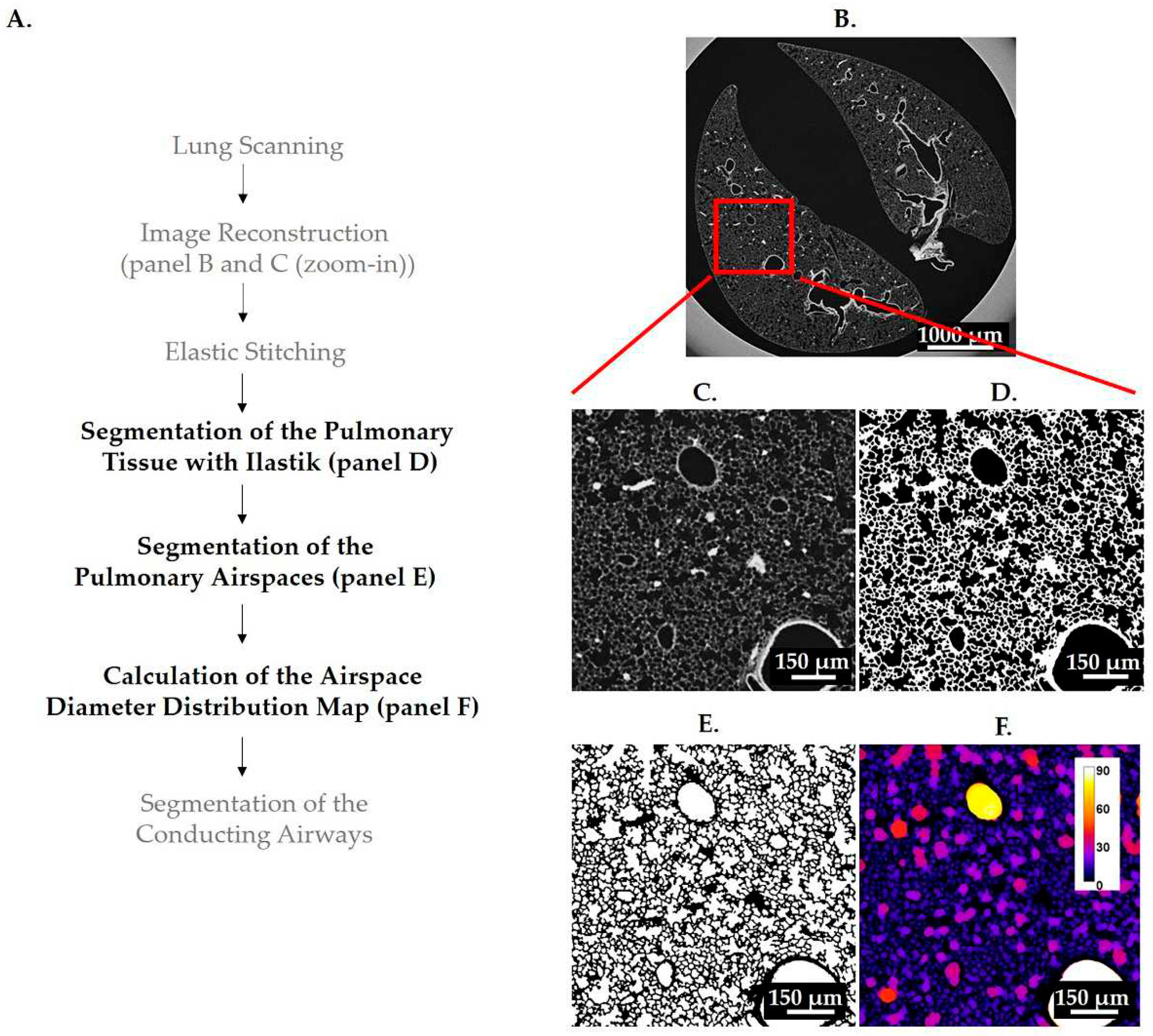
Figure 2.
Illustration of the parameters used in the statistical analysis. Different parameters of fit curves were assessed to determine the difference between βENaC-Tg/elastase-instilled- and control-samples: peak height and peak position (A), peak width and the position of the left and right shoulders at half peak height (B) and area under the curve left and right of the intersection (C, D).
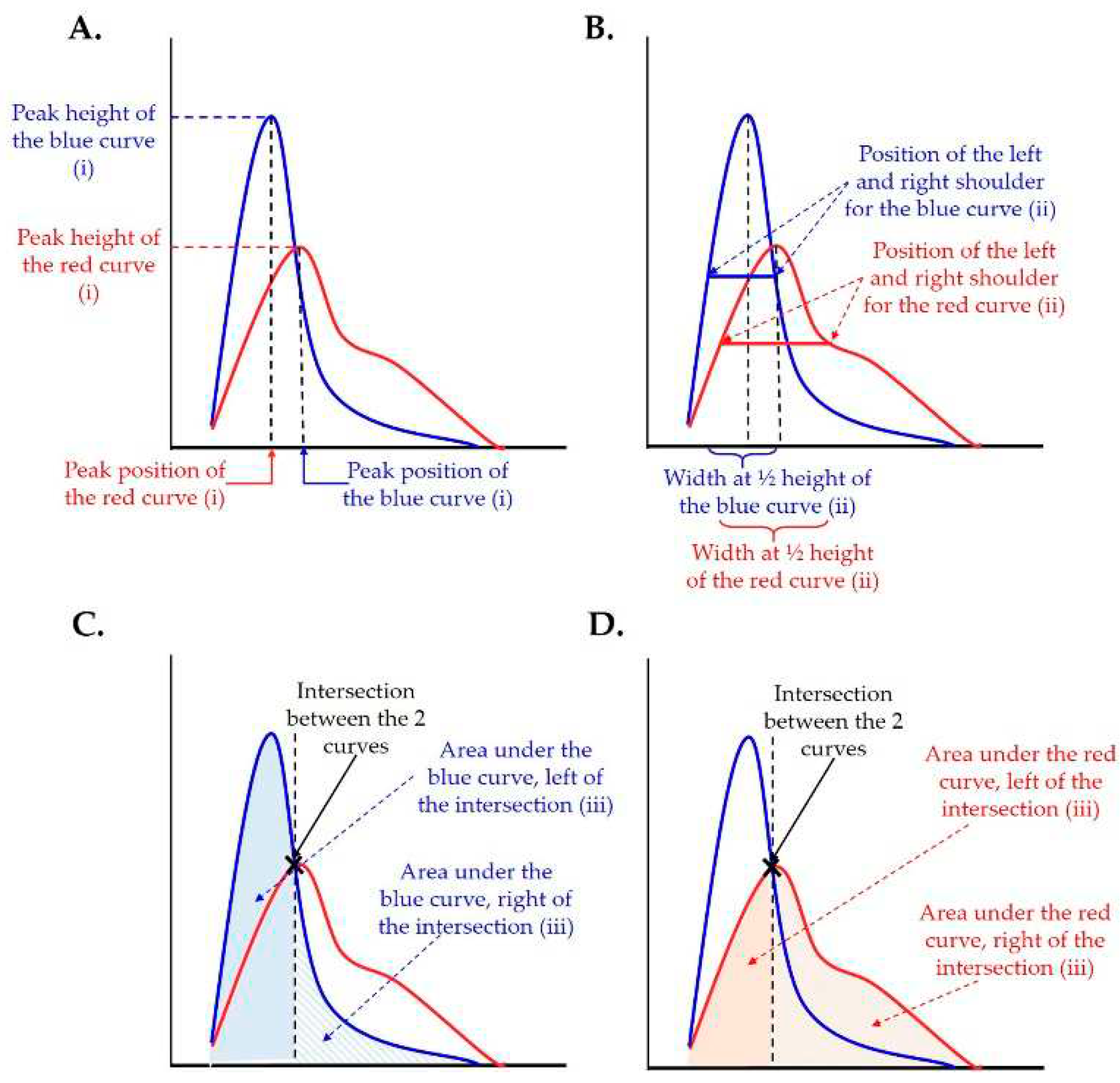
Figure 3.
Schematic representation of an airway diameter map. At every voxel, a sphere with the maximal diameter is fitted into the airspace (different diameter spheres are represented with different colors: blue, orange and white). Afterwards gray value that is equal to the diameter of the sphere is assigned to the voxel. We gain a map where the particular airspace diameter is encoded in every voxel. Voxel-counting is performed for every gray value and presented as a histogram “number of voxels” (voxel count) over “diameter of the airspace where the voxels are residing in.”.
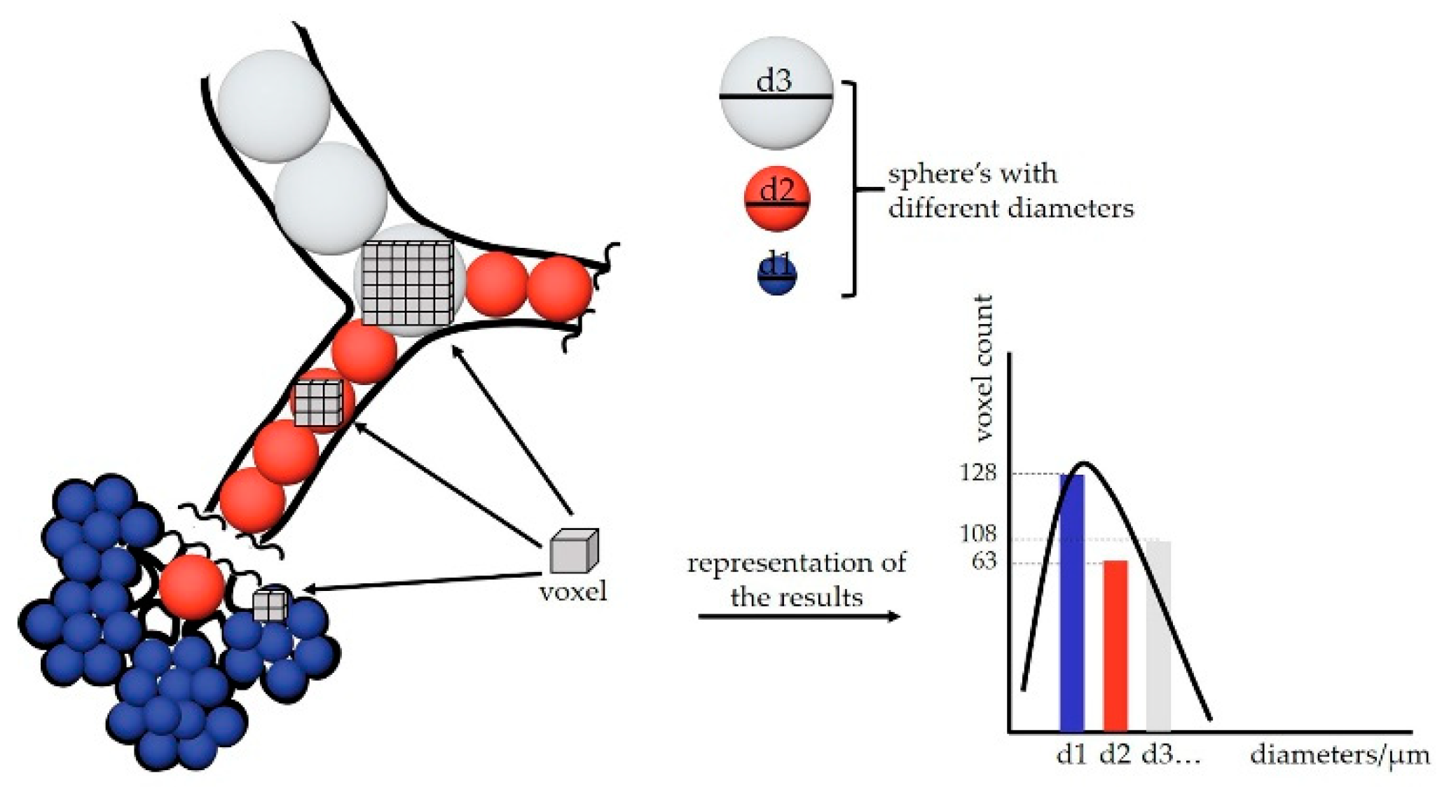
Figure 4.
Imaris illustration of conducting airways. The conducting airways, isolated with diameter threshold of 88 μm (A), 100 μm (B) and 112 μm (C) were visualized in Imaris and the overlap between three different thresholds is shown in (D). A threshold of 100 μm was chosen as the correct threshold. By applying a threshold that is too low, e.g., 88 μm, we obtain the alveoli together with the conducting airways (A, red circles). On the other hand, by applying a threshold that is too high, e.g., 112 μm, we are missing some parts of the conducting airways (C, white arrows). The scale bar is shown in every image on the bottom, while the color bar indicating diameter sizes in μm is shown in top right corner of image (A). The color of each channel in (D) is shown in the upper right corner (112 in red, 100 in yellow and 88 in blue) and the merges are indicated in the top of the image (white/gray for the merge of all 3 thresholds and turquoise for the merge of threshold 88 and 100). Threshold (Th).
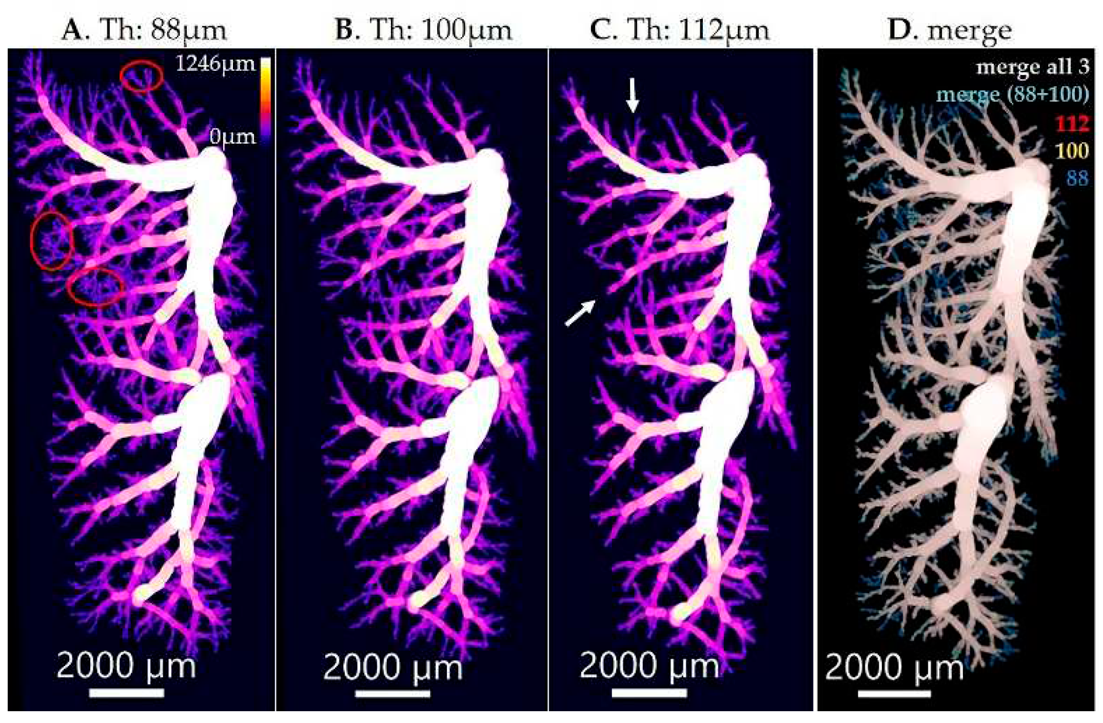
Figure 5.
Separation of the gas-exchange area from the conducting airways in healthy mouse lung from pnd36. The illustration of the entire lung (A, left panel) and different lung compartments, conducting airways (A, middle panel) and gas-exchange area (A, right panel), were prepared in Imaris. The calibration bar showing the color code for the airspace diameter sizes is shown in the bottom left corner of the left panel and the scale bar showing the image size is shown in the bottom right corner of the right panel). The thickness of airspaces residing in gas-exchange area and conducting airways is shown as fits of histogram distributions of voxel counts (B, C) and probabilities (D, E) over airspace diameter (µm). The results are shown with a solid, blue line for conducting airways and with a dashed, red line for gas exchange area. As the curves for conducting airways are not well visible in graphs (B) and (D) due to y-scale range, the zoom-in into conducting airways curves are shown in (C) and (E). The position of maximal curve’s peak, representing the most frequent airspace diameter, is shown with the black dotted line and the value of airspace diameter associated with the peak is labeled in blue for the conducting airways and red for the gas-exchange area.
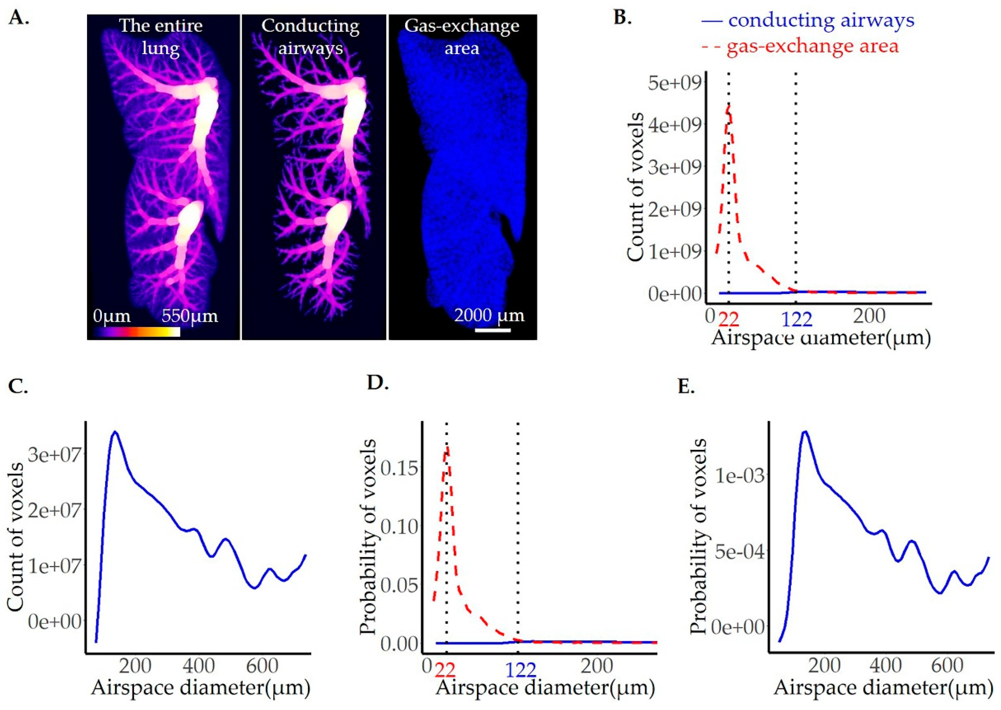
Figure 6.
Comparison of control and βENaC-Tg mice lungs with CF-like disease from pnd36. One representative lung slice from the ctrl (A, upper panel) and βENaC-Tg (A, lower panel) mice are shown. The thickness of pulmonary airspaces is shown as fits of histogram distributions of voxel counts (B, C) and probabilities (D, E) per airspace diameter (µm) of the entire lung. A total of 3 ctrls (solid, blue line) and 3 βENaC-Tg (dashed, red line) lungs were analyzed (B, D). The average per group (ctrl and βENaC-Tg) is shown in (C, E). The position of the peaks, representing the most frequent airspace diameters, are labeled with the black dotted lines and the values of the peak positions are given in blue for the ctrl and red for the βENaC-Tg groups. ctrl = control.
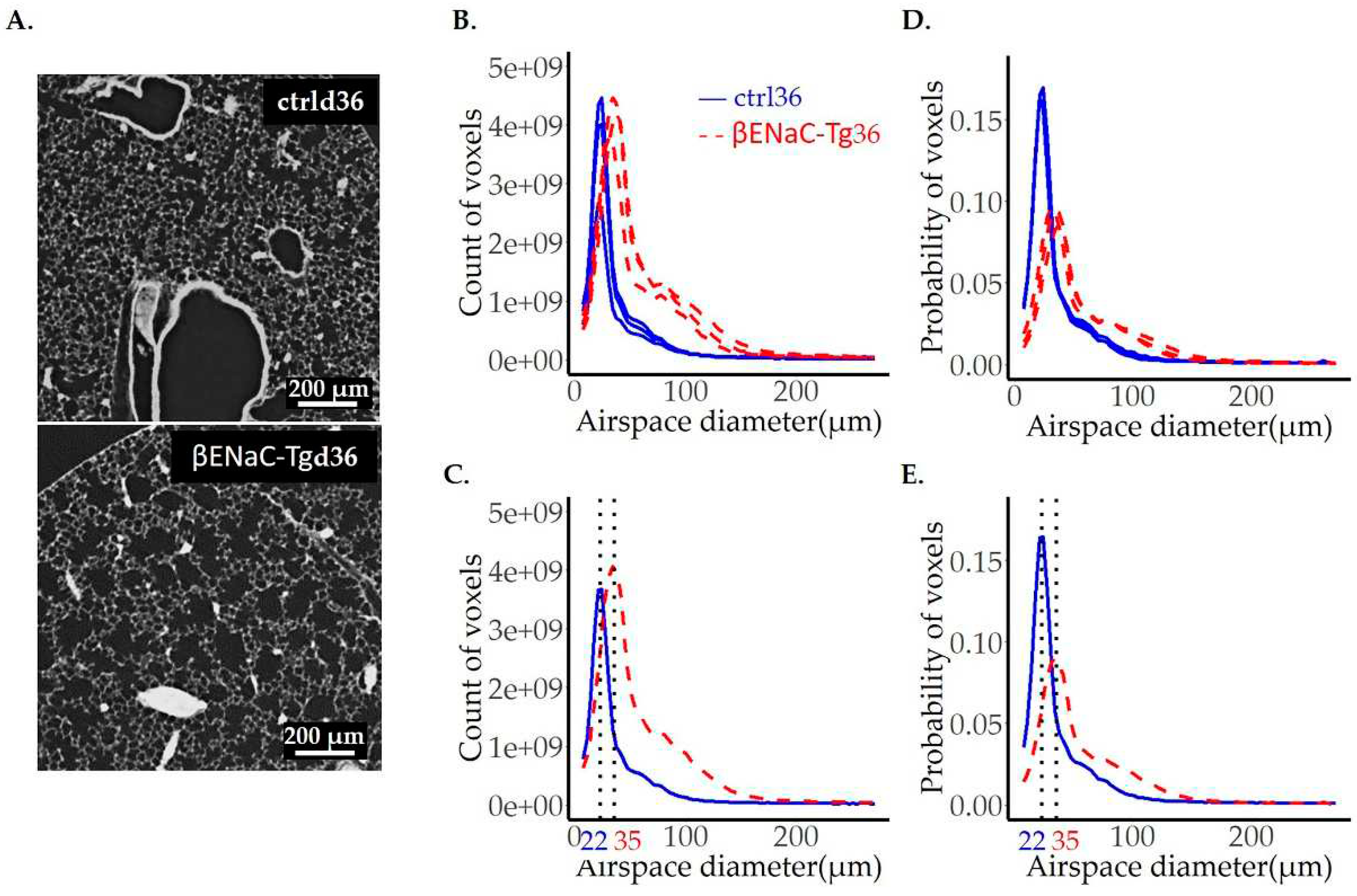
Figure 7.
Comparison of adult mice lungs instilled with saline (ctrl) or elastase (El). One representative lung slice from the ctrl (A, upper panel) and El (A, lower panel) mice are shown. The diameter of pulmonary airspaces is shown as fits of histogram distributions of voxel counts (B, C) and probabilities (D, E) per airspace diameter (µm) of the entire lung. The total of 3 ctrls (solid, blue line) and 3 elastase (dashed, red line) lungs were analyzed and illustrated in (B, D), while the average per group (ctrl and elastase) is shown in (C, E). The position of the peak, representing the most frequent airspace diameter, is shown with the black dotted line and the value of airspace diameter associated with the peak is the same in both groups and is labeled in black. The beginning of the shoulder is shown with the black arrows in (C, E).
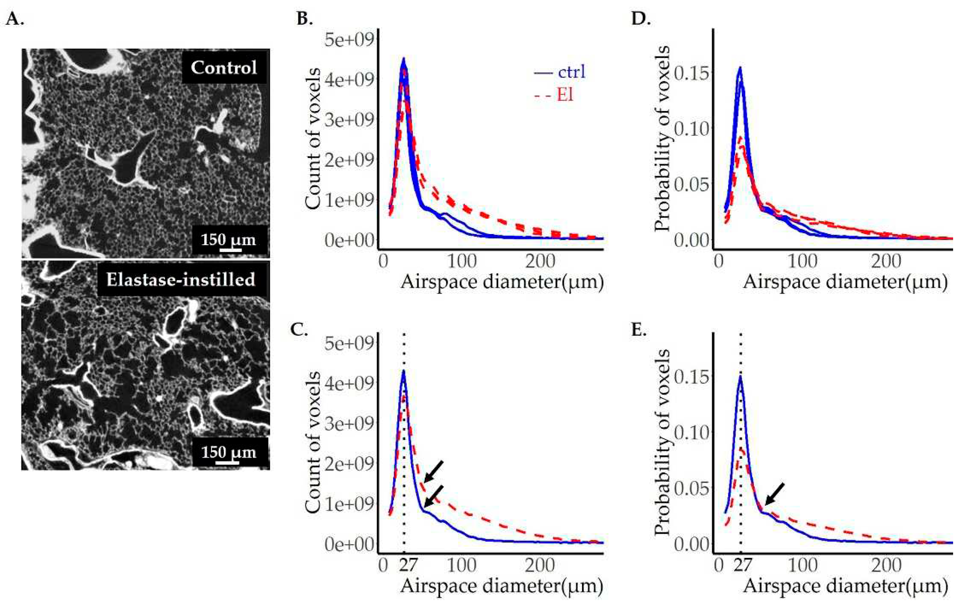
Figure 8.
Comparison of image analyses on images obtained by µCT and SRXTM (TOMCAT). To compare the quality of results obtained by μCT to our gold standard SRXTM, three left lungs were scanned with both setups. A representative lung slice from the ctrl (upper panels) and two elastase instilled lungs (El-1 and El-2) (middle and lower panels) imaged by SRXTM (left panels) or µCT (right panels) are shown in (A). The diameter of pulmonary airspaces is plotted as fits of histogram distributions of probabilities (B-D) over airspace diameter (µm). The results obtained by image analysis of SRXTM datasets are shown in blue, the ones obtained by μCT in red. The position of the peak, representing the most frequent airspace diameter, is shown with the black dotted line. The values of airspace diameters associated with the peak are shown in blue for TOMCAT and red for the μCT. The beginning of the shoulder is labeled with the black arrows in (B-D).
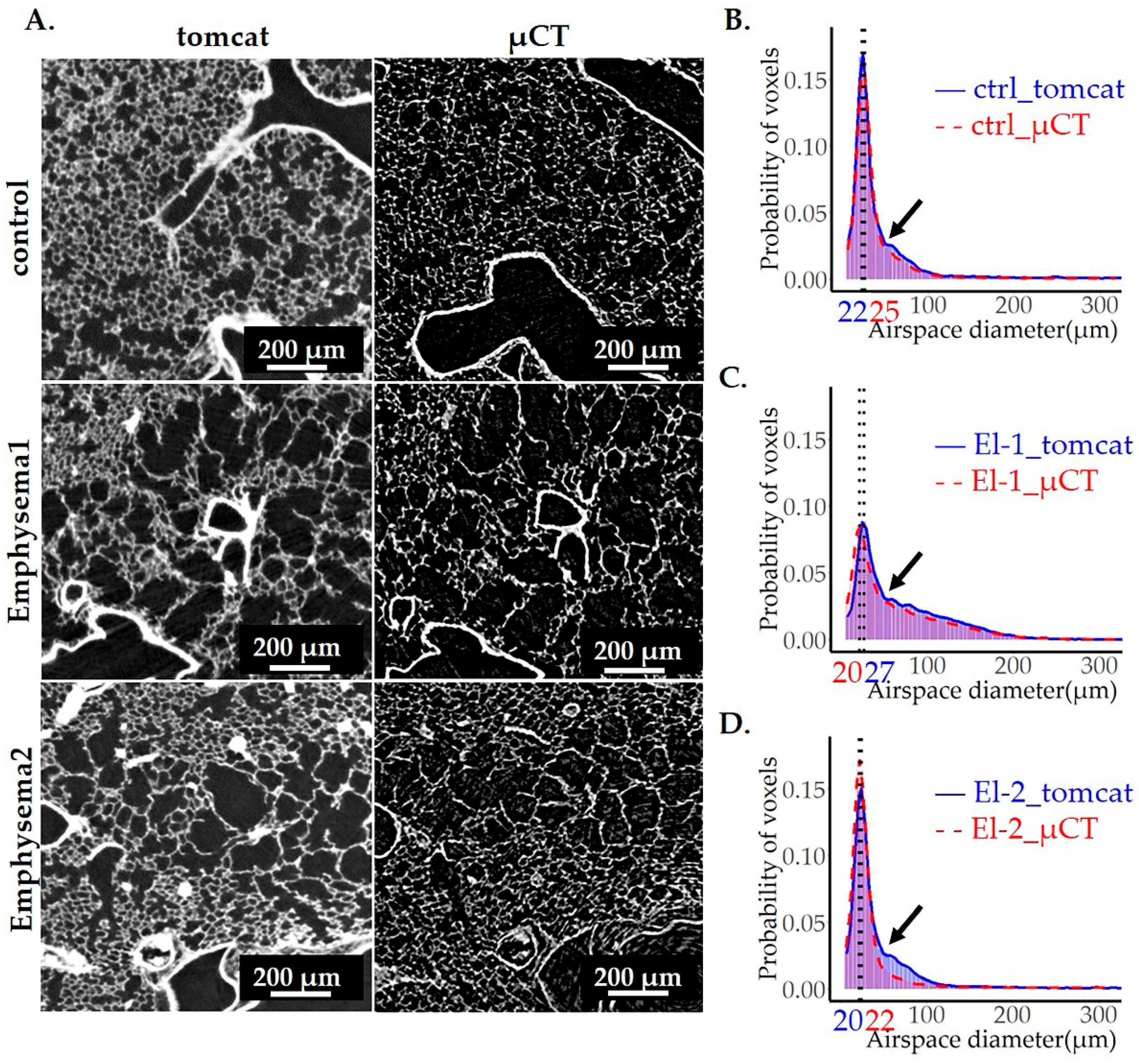

Table 1.
Comparison of count and probability distributions between the conducting airways and gas exchange area for the control sample from pnd36.
Table 1.
Comparison of count and probability distributions between the conducting airways and gas exchange area for the control sample from pnd36.
| Surface under the curve# | |||||||
| Peak position (µm) |
Peak height |
Peak width at ½ peak height (µm) | before the curve’s intersection | After the curve’s intersection | Volume of airspaces (μm3) | ||
| Count | CA | 121.6 | 3.6E+07 | 160.3 | 2.9E+08 | 1.8E+09 | 3.08E+10 |
| GEA | 22.0 | 4.5E+09 | 17.3 | 1.4E+10 | 1.0E+10 | 3.54E+11 | |
| Probability | CA | 121.6 | 1.4E-03 | 160.3 | 0.02 | 0.06 | |
| GEA | 22.0 | 0.2 | 17.3 | 0.6 | 0.3 | ||
CA = conducting airways; GEA = gas exchange area (lung parenchyma); # The surface under the curve is a direct measure of the airspace volumes.
Table 2.
Comparison of count and probability distributions between the ctrl and βENaC-Tg samples from pnd36.
Table 2.
Comparison of count and probability distributions between the ctrl and βENaC-Tg samples from pnd36.
| Surface under the curve# | |||||||
| Peak Position (µm) |
Peak height |
Peak width at ½ peak height (µm) | before the curve’s intersection | After the curve’s intersection | Volume of airspaces (μm3) | ||
| Count | ctrl | 22.0 (0.0) | 3.8E+09 (9.5E+08) | 17.1 (0.3) | 1.2E+10 (3.0E+09) | 1.0E+10 (2.3E+09) | 3.2E+11 (7.7E+10) |
| βENaC-Tg | 35.0 (5.6) | 4.1E+09 (2.8E+08) | 30.0 (1.9) | 9.2E+09 (9.4E+08) | 3.6E+10 (5.8E+09) | 6.6E+11 (7.3E+10) | |
| p | 0.02* | 0.6 | 0.0003*** | 0.2 | 0.002** | 0.005** | |
| Probability | ctrl | 22.0 (0.0) | 0.17 (0.003) | 17.1 (0.3) | 0.5 (0.01) | 0.5 (0.01) | |
| βENaC-Tg | 35.0 (5.6) | 0.09 (0.007) | 30.0 (1.9) | 0.2 (0.04) | 0.8 (0.04) | ||
| p | 0.02* | 4.6E-05**** | 0.0003*** | 0.0002*** | 0.0002*** | ||
ctrl = control; the standard deviation is shown in brackets; p < 0.05*, p < 0.01**, p < 0.001***, p < 0.0001****, significant p values are shown in bold; # The surface under the curve is a direct measure of the airspace volumes.
Table 3.
Comparison of count and probability distributions between the control and elastase-instilled samples.
Table 3.
Comparison of count and probability distributions between the control and elastase-instilled samples.
| Surface under the curve# | |||||||
| Peak Position (µm) |
Peak height |
Peak width at ½ peak height (µm) | before the curve’s shoulder | curve’s shoulder till end | Volume of airspaces (μm3) | ||
| Count | ctrl | 26.9 (0.0) | 4.2E+09 (3.4E+08) | 13.1 (0.2) | 1.9E+10 (1.5E+09) | 1.0E+10 (1.5E+09) | 4.2E+11 (4.0E+10) |
| El | 26.9 (0.0) | 3.7E+09 (4.1E+08) | 18.0 (1.4) | 1.8E+10 (1.7E+09) | 2.5E+10 (1.3E+09) | 6.3E+11 (4.1E+10) | |
| p | 0.4 | 0.2 | 0.004** | 0.7 | 0.0002*** | 0.002** | |
| Probability | ctrl | 26.9 (0.0) | 0.15 (0.003) | 13.1 (0.2) | 0.6 (0.02) | 0.4 (0.02) | |
| El | 26.9 (0.0) | 0.09 (0.005) | 18.0 (1.4) | 0.4 (0.02) | 0.6 (0.02) | ||
| p | 0.4 | 6.6E-05**** | 0.004** | 0.0001*** | 0.0001*** | ||
ctrl = control; El = elastase instilled samples; The standard deviation is shown in brackets; p < 0.01**, p < 0.001***, p < 0.0001****, significant p values are shown in bold; # The surface under the curve is a direct measure of the airspace volumes.
Table 4.
Comparison of probabilities of airspace diameters obtained by image analysis of SRXTM and µCT datasets.
Table 4.
Comparison of probabilities of airspace diameters obtained by image analysis of SRXTM and µCT datasets.
| Surface under the curve | ||||||||
| Peak position (µm) |
Peak height |
Peak width at ½ peak height (µm) | before the shoulder | shoulder | After shoulder | |||
| ctrl |
SRXTM |
22.0 | 0.17 | 17.7 | 0.7 | 0.2 | 0.1 | |
| μCT | 24.8 | 0.16 | 19.1 | 0.7 | 0.2 | 0.1 | ||
| El-1 | SRXTM | 26.9 | 0.09 | 26.4 | 0.43 | 0.5 | 0.03 | |
| μCT | 20.3 | 0.08 | 27.8 | 0.46 | 0.5 | 0.03 | ||
| El-2 | SRXTM | 22.0 | 0.15 | 19.7 | 0.7 | 0.2 | 0.1 | |
| μCT | 20.3 | 0.16 | 19.8 | 0.8 | 0.1 | 0.1 | ||
No relevant differences were observed between the SRXTM and μCT scans, except of the shoulder of elastase treated sample El-2. The differences of the peak positions are appearing as large, but they are in the range of +/- 1 bin size of the histogram.
Disclaimer/Publisher’s Note: The statements, opinions and data contained in all publications are solely those of the individual author(s) and contributor(s) and not of MDPI and/or the editor(s). MDPI and/or the editor(s) disclaim responsibility for any injury to people or property resulting from any ideas, methods, instructions or products referred to in the content. |
© 2023 by the authors. Licensee MDPI, Basel, Switzerland. This article is an open access article distributed under the terms and conditions of the Creative Commons Attribution (CC BY) license (http://creativecommons.org/licenses/by/4.0/).
Copyright: This open access article is published under a Creative Commons CC BY 4.0 license, which permit the free download, distribution, and reuse, provided that the author and preprint are cited in any reuse.


