
Submitted:
27 June 2023
Posted:
28 June 2023
You are already at the latest version
Abstract
The evaluation of suitability for bioclimatic viticulture indices (BVIs) zones, as with any other crop, requires a well-founded knowledge of the spatial variability in climate data, which is also used to assess different grapevine cultivars and to delimit appropriate regions for vineyard production under the current climate and projected climate change. BVIs, on the other hand, are typically calculated using a small number of locations linked by climatic station sites or applied using a coarsely-resolution distributed dataset. Furthermore, often the methods applied to precisely delineate symmetrical regions are not appropriate to generate accurate maps. To provide an analysis using three temperature-based indices and the hydrothermal coefficient (HTC), quantifying their spatial variation, and representing the spatial patterns of each BVI throughout the Jabal Al Arab viticulture—one of the most important Syrian viticulture regions in the Eastern Mediterranean—daily temperature data from 15 meteorological stations and 57 rain gauges, considering the 1984–2014 period, and downscaled future scenarios (RCPs based on CanESM2), considering the 2016–2100 period, were utilized. The statistical method of each BVI was analyzed, and, later, they were mapped by using GIS and a hybrid interpolation (regression-kriging) approach. The regression fitting method revealed that the sum accumulation of heat and the hydro-thermal index during the growing season were highly related to elevation and distance to the seacoast variables; however, the viticulture zones varied spatially depending on which index was used and under suggested future scenarios compared to the current climate. The spatial distribution of climate in the Jabal Al Arab regions exhibits significant variability. The findings suggest that climate change projections indicate a prevalence of warmer conditions in the future. Under the RCP scenarios, the territory can be categorized into up to three bioclimatic classes for both the Heat Index (HI) and the Winter Index-Growing Degree Days (WI-GDD), in contrast to the current climate which has six classes. These results provide valuable insights into the suitability of viticulture within each climatic region and facilitate the identification of homogeneous zones. The utilization of consistent bioclimatic indices and an advanced hybrid interpolation method has enabled the delineation and comparison of bioclimatic variables of Jabal Al Arab with other regions worldwide. Such comparisons should be considered when selecting grapevine varieties and assessing the potential for grape production.
Keywords:
Grapevine (Vitis vinifera)
; hybrid Interpolation
; climate change
; CanESM2
; agro-climatic indices
; sustainable farming
; regression-kriging
; RCPs
; Syria.
1. Introduction
Grapevine (Vitis vinifera) holds significant cultural, ecological, and economic importance in the Mediterranean Basin, making it a major crop with the largest acreage among fruit products (Vivier and Pretorius, 2002; Ponti et al., 2018). The production of grapevines is influenced by various interconnected environmental conditions (Alsafadi et al., 2020), often encompassed by the term "terroir." While there is ongoing debate regarding its precise definition, most definitions attempt to capture the combination of micro-climatic factors, soil characteristics, topography, geology, and their intricate interrelationships (Huggett, 2006; Jackson and Lombard, 1993; Cardoso et al., 2019). The International Organization of Vine and Wine (OIV) has defined "terroir" as having a geographical dimension, emphasizing the necessity for zoning and delimitation, particularly with regard to agroecological factors such as climate and soil (OIV, 2012). However, in research aimed at determining the suitability of specific sites for vineyards or the cultivation of particular grapevine varieties, the influence of meteorological elements in the delimitation of zones should carry more weight than soil characteristics (OIV, 2012).
Since temperature variability can significantly impact viticultural areas at different scales, various temperature-based Bioclimatic viticulture indices (BVIs) have been developed. These include the Winkler Index (WI-GDD) (Amerine and Winkler, 1944), the Huglin Index (Huglin, 1978), the cool night index (CI) (Tonietto and Carbonneau, 2004), and the Hydrothermal Coefficient (HTC) which integrates the effects of temperature and precipitation during the growing season (Branas et al., 1946). BVIs have been extensively studied in viticultural regions worldwide using diverse approaches. Examples include Argentina (Cabré et al., 2016; Cabré and Nuñez, 2020), Australia (Hall and Jones, 2010; Jarvis et al., 2017), Europe (Santos et al., 2012), New Zealand (Anderson et al., 2012), Croatia (Omazić et al., 2020), central Chile (Montes et al., 2012), western USA (Jones et al., 2010), Hungary (Gaál et al., 2012), Serbia (Vuković et al., 2018), Romania (Patriche et al., 2022), the province of Quebec in Canada (Jones, 2018), the State of Washington and parts of northeast Oregon in the USA (Badr et al., 2018), and even globally (Tonietto and Carbonneau, 2004). Smaller regions such as the Miño river valley in Spain (Blanco-Ward et al., 2007), Turkey's Black Sea Region (Köse, 2014), Portuguese Douro valley region (Blanco-Ward et al., 2019; Santos et al., 2011), the western slopes of Jabal Al Arab in Syria (Alsafadi et al., 2020), the Apulian region in Italy (Alba et al., 2021; Gentilesco et al. 2023), and Santorini Island in Greece (Xyrafis et al., 2022) have also been studied.
As part of the eastern Mediterranean region, the agricultural sector in southern Syria faces significant challenges related to various environmental issues. These challenges include soil erosion (Mohammed et al., 2020), the impact of climate change on agricultural production (Alsafadi et al., 2023a), and the negative consequences of unsustainable agricultural practices on soil health (Mohammed et al., 2021). Among the agricultural activities in this region, viticulture holds great importance as it supports the livelihood of the local population and contributes to food industries such as grape-wines, molasses, and raisins. However, similar to other agricultural sectors, viticulture also encounters several environmental problems, including unsustainable management practices (Alsafadi et al., 2020) and difficulties associated with the availability of soil micronutrients for vineyard cultivation (Mohammed et al., 2022). Research conducted by Mohammed et al. (2022) revealed that the majority of studied soils in southern Syria, specifically for vineyard cultivation, exhibit micronutrient concentrations below the critical level. To promote sustainable viticulture practices, Alsafadi et al. (2020) developed new maps that analyze optimal regions for economically viable viticulture production in this area. These maps incorporate climate-viticulture indices, soil requirements, and other topographic indicators to identify suitable locations for cultivating vineyards. These maps aim to assist decision-making processes in selecting new cultivation sites and support the development of sustainable viticulture practices in the region.
To enhance the management of local viticultural regions in response to global warming and climate change, it is crucial to have high-resolution data that accurately depict the spatial distribution BVIs (Hall and Blackman, 2019; Sturman et al., 2017; Le Roux et al., 2017). General circulation models (GCM) of climate change often lack the precision required to delineate the variability of BVIs at the local level, which typically operates at approximately 300 km spatial resolution. Additionally, the calculation of BVIs often relies on a small number of locations connected through climatic station sites or coarse-resolution distributed datasets. Consequently, the methods employed to precisely delineate symmetrical regions may not generate accurate maps. Several algorithms and methods have been employed to generate fine-scale gridded data for BVIs. These include geostatistical approaches (Morari et al., 2009), dynamical and statistical downscaling (Blanco-Ward et al., 2019; Hofmann et al., 2022), and dynamical and geostatistical techniques (Le Roux et al., 2016). Remote sensing-based modeling utilizing MODIS-land surface temperature (LST) has been utilized (Zorer et al., 2012), along with downscaling of MODIS-LST through machine-learning regression models (Morin et al., 2020) and statistical methods such as multivariate linear regression and non-linear support vector regression (Le Roux et al., 2017). Other methods employed include the regression-kriging (RK) method (Moral et al., 2014) and the Weather Research and Forecasting model WRF (Sturman et al., 2017). In general, hybrid interpolation algorithms are preferred, particularly when incorporating auxiliary information and interpolating the models' residuals. Numerous studies have indicated that the RK technique is suitable for this purpose (Moral et al., 2014; Alsafadi et al., 2021; Alba et al., 2021). By utilizing these advanced methods, it becomes possible to generate accurate and detailed maps of BVIs, enabling better understanding and management of viticultural regions in the face of climate change.
Our study focuses on the mapping of precipitation and temperature-based BVIs at a fine resolution during the growing seasons in the prominent viticulture regions of Jabal Al Arab, situated in the Eastern Mediterranean. The mapping covers the period from 1984 to 2014 and incorporates downscaled climate change scenarios based on the CanESM2 model and three Representative Concentration Pathways (RCPs) from 2015 to 2100. To achieve this, we employed the Regression-Kriging (RK) model, allowing us to generate maps at a high resolution of 1000-meter intervals. For the implementation of the RK model, we utilized daily observed temperatures and applied the regression method. To enhance the accuracy of the model, we conducted a regression analysis of BVIs using a range of terrain characteristics obtained from a Digital Elevation Model (DEM) and auxiliary information. This approach has been successfully employed in previous studies and demonstrated superior performance compared to a simple regression model. By utilizing the RK model and incorporating various terrain characteristics and auxiliary information, we aim to produce highly detailed maps of BVIs, providing valuable insights into the viticulture regions of Jabal Al Arab. Additionally, we extended our analysis to include climate change projections based on the CanESM2 model and RCPs, enabling us to assess the potential impacts of future climate scenarios on viticulture in the region.
2. Materials and Methods
2.2. Study area, data collection, and preliminary analysis
The study area under investigation is situated in the Eastern Mediterranean, specifically in southwestern Syria and northern Jordan. Geographically, it lies between latitudes 32°18' N and 33°13' N, and longitudes 36°20' E and 37°02' E, encompassing an area of 3,458 km2 (Figure 1a). The climate in this region is characterized as continental, with cold and wet winters, and hot and dry summers. In July, average temperatures during the summer range between 18°C and 32°C, while in January, winter temperatures average between 3°C and 10°C (Figure 1b). The average annual precipitation in the region is 350 mm, with the maximum recorded rainfall being approximately 570 mm in the elevated area (Figure 1a). The majority of rainfall is concentrated in the winter season, with the mean monthly precipitation in February ranging from 10 mm to 145 mm. Based on the Köppen-Geiger classification, the central and western hilly regions of the study area fall within the temperate-wet climatic zone, whereas the eastern part is characterized by a desert (arid) or semi-arid (continental or steppe) climate. The altitudes in the region vary from 696 m in the western part to 1795 m above sea level in the central part (Tall Qeni). The area holds significant importance as a viticulture region in the Eastern Mediterranean, with a total viticultural area of approximately 10,125 ha in 2015. According to the Syrian Ministry of Agriculture and Agrarian Reform (SMOAAR, 2015), the region is the second most important in terms of viticulture, following apples. Vineyards are a crucial source of income for thousands of families, with an annual production of no less than 40,000 tons. The cultivation of vineyards in this region is deeply rooted in the region's economic heritage, passed down from previous generations.
In this study, the modeling of the BVIs gridded data at a fine spatial resolution of the study area was based on in-situ data from several sources, which can be explained as follows:
2.2.1. Observed air temperature and precipitation
To fulfill the main objectives of our research, we utilized in-situ data obtained from various sources, including 57 rain gauges and 15 climatic stations. These data were sourced from the Syrian Meteorological Authority (SMA), SMOAAR, and the Jordan Meteorological Department (JMD) database. The selection of stations took into consideration their location, both within and outside the study area, as depicted in Table 1. Monthly data spanning from 1984 to 2015 were collected for analysis. During the data preparation phase, we included stations with observations covering a minimum of 20 years to ensure data reliability. To address any missing values and ensure uninterrupted data acquisition, gap-filling techniques were applied. Specifically, we utilized 7 rain gauges with complete data and 9 gridded points of temperature variables from the NASA Power Data, which have a resolution of 0.5°arc degree, as reference data for correction, gap filling, and homogeneity testing. Regardless of the spatial interpolation method employed, careful data preparation and handling were necessary. This involved removing outliers, selecting candidates and reference stations, filling data gaps, and conducting homogeneity tests. It is important to note that when dealing with data from multiple sources, each with its own settings, these steps are crucial to obtain high-quality data for reliable climate assessment. To ensure data quality, a rigorous procedure was implemented, which included analyzing the difference series between candidate stations and their neighboring stations through pairwise comparisons. Missing values were interpolated using simple linear regression. Furthermore, the Standard Normal Homogeneity Test (SNHT), as proposed by Alexandersson (1986), was applied to assess data homogeneity. For detailed information on the quality control and homogeneity testing process, refer to the attached documentation for the AnClim software (Štěpánek et al., 2009).
2.2.2. CIMP5 climate projection (CanESM2)
The large-scale standardized climatic variables of CanESM2 (the 2nd Generation Canadian Earth System Model) and the NCEP (National Centers for Environmental Prediction) reanalysis dataset were used to assess the current climate and projected climate change under the Representative Concentration Pathways (RCPs). These datasets are available from the Canadian Climate Data and Scenarios website (http://climate-scenarios.canada.ca) for the baseline climate period of 1961-2005 and future scenarios from 2006-2100 under three RCPs (RCP2.6, RCP4.5, and RCP8.5). The spatial resolution of the data is approximately 2.81 degrees, with longitude and latitude values relatively fixed. To represent nearly observed station data in the study area, the "BOX_014X_44Y" grid cell from CanESM2 was selected. However, due to the coarse spatial resolution of General Circulation Models (GCMs), their applicability in impact evaluation research, environmental planning, adaptation, and decision-making at regional and local scales is limited. Furthermore, uncertainties and biases associated with GCMs increase when compared to regional and local scales, further limiting their usefulness in local-scale assessments and environmental planning studies. To address this, a downscaling process was employed to increase spatial resolution, reduce potential biases, and provide finer spatial information. The Statistical DownScaling Model (SDSM) (Wilby et al. 2002) was adopted to downscale the outputs from CanESM2. This method involves statistically fitting a relationship between local-scale climatic variables (predictands) and large-scale climatic variables (predictors) using a multiple regression model and bias correction methods (Tavakol-Davani et al. 2012; Meenu et al. 2013). In this study, the SDSM software was used to downscale the CanESM2 outputs. The observed monthly precipitation data from 57 rain gauges and average, maximum, and minimum temperatures from 15 synoptic weather stations were utilized. Additionally, 26 predictors from the NCEP reanalysis data and CanESM2 (see Table 1 in Gebrechorkos et al. 2019) were imported into the software for model fitting, validation, and future projections.
2.3. Bioclimatic Viticulture indices (BVIs)
Five BVIs were calculated to assess the impact of climate change on viticulture in the Eastern Mediterranean:
(i) The Hydrothermal Coefficient (HTC) was introduced by Branas et al. (1946) as a measure that combines the influence of seasonal precipitation and temperature specifically during the growing season. Its purpose is to assess water availability for vineyards and determine the suitability of rainfed viticulture (Mesterházy et al., 2014). In areas where HTC values fall below 0.5 mm/°C, grape production can only be sustained with high air humidity or irrigation. The HTC ranges from 1.5 to 2.5 mm/°C, with an optimal value of 1.0 mm/°C (Mesterházy et al., 2014).
P represents the rainfall during the growing season in millimeters, and GDD denotes the cumulative effective degree days above 10°C.
(ii) The Winkler Index (WI-GDD) is commonly used to estimate the heat accumulation during the growing season for vineyards. Traditionally, this index calculates the total daily average temperatures from April to the end of October, using a base temperature of 10°C, as proposed by Amerine and Winkler (1944). In our study, due to the warm climate in the region compared to higher altitude areas, we extended the calculation period from March to the end of September. The WI-GDD can be expressed as follows:
(ii) The Huglin Index (HI) was developed by Huglin (1978) and is calculated similarly to the WI-GDD, but with a greater emphasis on maximum temperature and an adjustment based on latitude, specifically the length of the day coefficient (Huglin, 1978). The HI provides more detailed information on the sugar potential of specific grape varieties and offers qualitative insights when combined with the values of the CI cool night index (Tonietto and Carbonneau, 2004). Jones et al. (2009) and Hall and Jones (2010) have updated the HI formula to accommodate all latitudes, considering the months from April to September in the Northern Hemisphere and excluding October, as they believe that the values become less significant during the harvest period (Jones et al., 2010; Anderson et al., 2012). In this study, we begin accumulating daily average temperatures from March, using a coefficient length of the day of "d=1".
((v) The Cool Night Index (CI) was developed by Tonietto and Carbonneau (2004) to assess the degree of coolness during nighttime by considering the average minimum temperatures in the ripening month, typically September in the Northern Hemisphere. This climatic factor significantly influences grape and wine characteristics, including color and aromas. The CI is particularly useful for evaluating the qualitative aspects of wine grapes, specifically the presence of secondary metabolites like aromas and polyphenols in grape juice (Kliewer, 1973). To calculate CI, the minimum air temperatures in September are averaged and expressed in degrees Celsius for the Northern Hemisphere. In the Southern Hemisphere, the calculation involves averaging the minimum air temperatures in March, also expressed in degrees Celsius (Tonietto and Carbonneau, 2004). These climate-viticulture indices, which also include the previously mentioned ones, enable the assessment of the optimal climatic suitability in terms of heat, water availability, phenological development throughout the growing season, and ripening conditions (Fraga et al., 2014). Please see Table 1 for more details regarding the climate-viticulture indices zones.

Table 2.
The applied BVIs in this study and their class interval.
| BVIs | Unit | Class of BVIs, and class interval | Reference | |
|---|---|---|---|---|
| Growing season temperatures (GST) |
°C | Cool (C) | 13-15 | (Jones, 2006) |
| Temperate (T) | 15-17 | |||
| Warm (W) | 17-19 | |||
| Hot (H) | 19-24 | |||
| Hydrothermal Coefficient (HTC) |
- | Excessively dry (ED) | <0.25 | (Branas et al. 1946) |
| Dry (D) | 0.25–0.5 | |||
| Moderately dry (MD) | 0.5–1.5 | |||
| Moderately wet (MW) | 1.5–2 | |||
| Wet (W) | 2–2.5 | |||
| Excessively wet (EW) | >2.5 | |||
| Winkler Index- growing degree days (WI-GDD) |
GDD | Too cold (TC) | <850 | (Amerine and Winkler 1944) |
| Cold (C) | 850–1390 | |||
| Moderately cold (MC) | 1391–1670 | |||
| Warm (W) | 1671–1940 | |||
| Moderately warm (MW) | 1941–2220 | |||
| Hot (H) | 2221–2700 | |||
| Too hot (TH) | >2700 | |||
| Huglin Heliothermal index (HI) |
GDD | Too cold (TC) | <1200 | (Huglin, 1978) |
| Very cool (VC) | 1200–1500 | |||
| Cool (C) | 1500–1800 | |||
| Temperate (T) | 1800–2100 | |||
| Temperate warm (TW) | 2100–2400 | |||
| Warm (W) | 2400–2700 | |||
| Very warm (VW) | 2700–3000 | |||
| Too hot | >3000 | |||
| Too cold (TC) | <1200 | |||
| Cool Night Index (CI) | °C | Very cool nights (VCN) | <12 | (Tonietto and Carbonneau, 2004) |
| Cool nights (CN) | >12 ≤ 14 | |||
| Temperate nights (TN) | >14 ≤ 18 | |||
| Warm nights (WN) | >18 | |||
(vi) The Growing Season Temperatures (GST) is a climate-maturity zoning system created by Jones (2006) to classify regions based on the correlation between phenological needs and growing season temperatures. It encompasses a range of climates, from cool to hot, to cultivate high-quality grapevines in globally recognized regions and for commonly grown grape varieties. The GST system assists in identifying the favorable climate conditions required for optimal grapevine growth and maturity during the growing season.
2.4. Fine-scale modeling of BVIs using regression-Kriging (RK)
To accurately produce regional zones of BVIs at a fine spatial resolution, it is necessary to obtain BVIs for each pixel with fixed horizontal spacing grids, taking into consideration the environmental lapse rate. The environmental lapse rate represents the ratio of BVIs' change with variation in altitude, which leads to variations in temperature accumulation during the growing season due to complex terrains. Typically, these procedures involve using a digital elevation model (DEM) and employing local regression equations and hybrid interpolation methods such as Regression-Kriging (Moral et al. 2014; Alba et al. 2021; Alsafadi et al. 2023b). Geostatistical interpolation approaches recognize that the geographical variation of any continuous variable, including each BVI, is often too irregular to be described by a simple mathematical function. Instead, a stochastic surface can better explain the variation. The Regression-Kriging (RK) method (Odeh et al. 1995, Hengl et al. 2007) is applied, where each BVI is independently determined using multivariate regression trend (MR), and the MR's residuals are added back in the next step. This process allows obtaining BVIs with fixed horizontal spacing grids at each unsampled pixel x based on the following equation:
where the regressions, rm(s), are fitted by the MR, and the MR's residuals, r(s), are predicted using Ordinary Kriging (OK) method. The predictions were expressed in the equation:
In equation (6), represents the predicted value of the BVIs at unsampled pixel x. It is obtained by adding the regressions, , fitted by the multivariate regression trend (MR), with the predicted residuals, , using the Ordinary Kriging (OK) method. The predictions are expressed as follows:
represents the estimation at a specific site (x), are the unstandardized coefficients of the MR, is the predictor (value of the independent variable) at the same site. is the number of predictors used in RM models, is the weight fixed by applying the OK method of the MR residuals, , for neighboring observed points.
In equation (7), represents the estimation at a specific site (x). The equation is comprised of two main parts. The first part is the sum of the products of unstandardized coefficients, , and predictors, , at the same site. This represents the contribution of the multivariate regression trend (MR) to the estimation. The sum is performed over all p predictors used in the MR models. The second part is the sum of the products of weights, , and the predicted residuals, , obtained from applying the Ordinary Kriging (OK) method to the MR residuals. This represents the contribution of the spatial interpolation of the residuals to the estimation. The sum is performed over n neighbouring observed points. Together, these two parts combine to provide the estimation at the specific site x.
To achieve this, the elevation data for the study area was obtained by calculating and extracting it from the Digital Elevation Model (DEM) provided by the U.S. Geological Survey's Center for Earth Resources Observation and Science (EROS) Archive - Digital Elevation - Global (GTOPO30) within the HYDRO1k project data (Danielson and Gesch 2011). The DEM had a horizontal grid spacing of 30 arc-seconds, which corresponds to approximately 1 km resolution. Geographic data such as longitudes, latitudes, and distances to the sea coastline were also collected. Additionally, MODIS cloud cover data were acquired for the study area, which was used for precipitation modeling. These data, along with the elevation data, were utilized in fitting the multivariate regression (MR) models using the principal component method. This approach helped address the issue of multicollinearity that can arise when using correlated variables in the MR method. It should be noted that the RK method, which was employed for spatial interpolation, tends to provide more accurate predictions when the variables are available at all locations within the region. In this study, regular gridded data at a resolution of 1000 meters were used to obtain the BVIs for the entire study area, while station-based BVI estimates were obtained for a fixed horizontal spacing grid, resulting in a continuous surface. This approach allowed for the determination of BVI values for each smallest resolution unit (pixel) within the study area. Four raster BVI models were created: one representing the current climate for the period of 1984-2014, and three models for different climate change scenarios (Representative Concentration Pathways - RCPs). All of the procedures described above were carried out using the geostatistical tool package within the ArcGIS 10.8 environment.
3. Results
3.1. Projected change in temperatures and precipitation
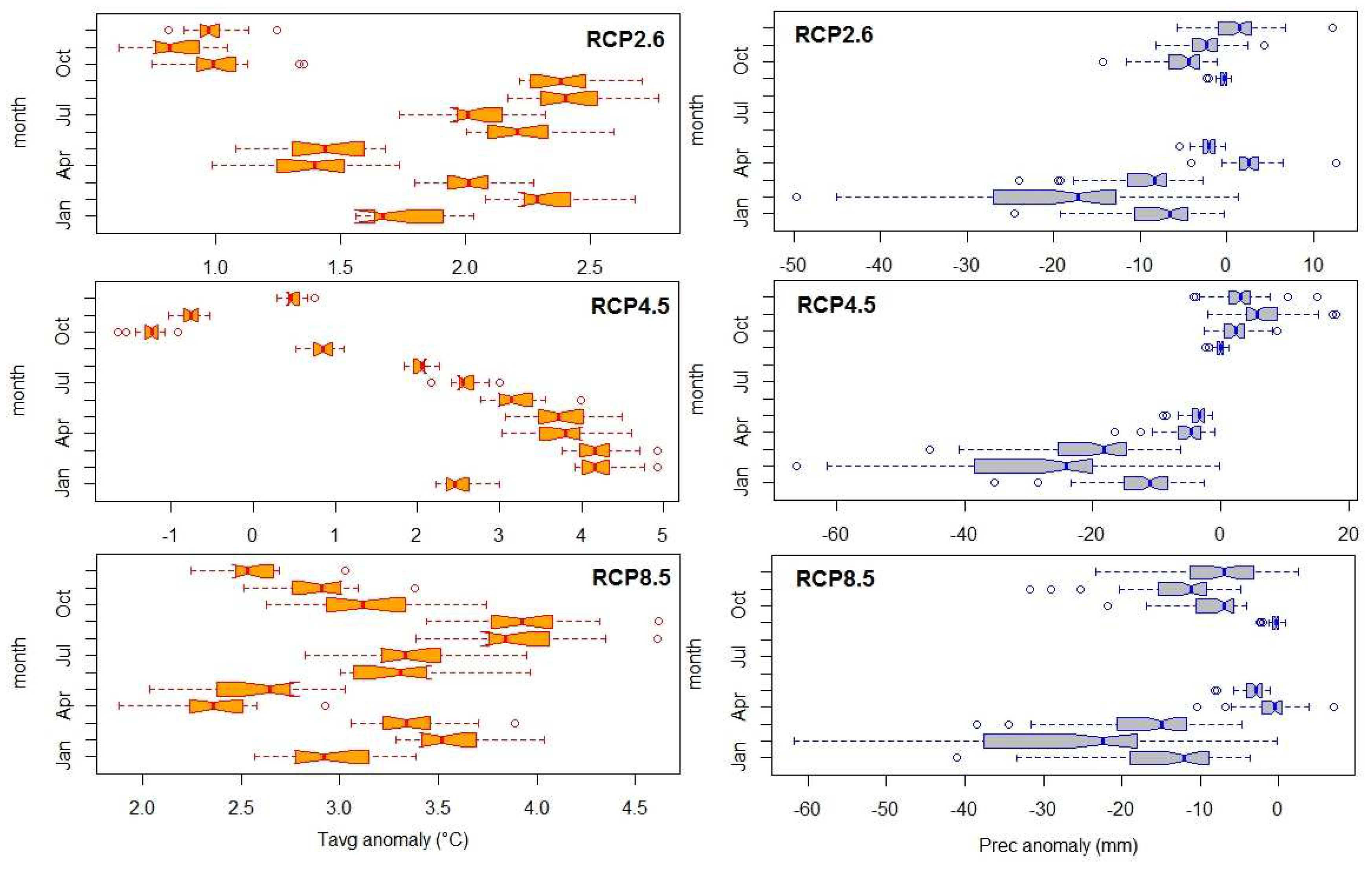
Estimates were conducted to assess the spatiotemporal variability of mean air temperature and annual precipitation anomalies under the CanESM2 projection for the period 2015-2100, considering three RCPs - RCP2.6, RCP4.5, and RCP8.5. The baseline period used for comparison was 1984-2014, and the analysis was carried out across 15 regions in southern Syria. The results reveal that under RCP2.6, the average anomalies in mean air temperature across all 15 stations were 1.73 °C. The highest average temperature anomaly was recorded in August (2.42 °C), while the lowest was observed in November (0.83 °C). These findings indicate that the average air temperature was higher than the baseline values across all regions. Similar patterns were observed for RCP4.5 and RCP8.5, with average anomalies of 2.13 °C and 3.16 °C, respectively, across all months. The highest average anomalies occurred in February and March, with values of 4.14 °C and 4.1 °C for RCP4.5, and in August and September, with values of 3.65 °C and 3.75 °C for RCP8.5. On the other hand, the lowest anomalies were observed in October, with a value of -1.25 °C for RCP4.5, and in April, with a value of 2.35 °C for RCP8.5. However, under RCP4.5, the anomalies in mean air temperature were negative in October and November across all regions, indicating that the temperature during these months became colder compared to the baseline values.
Regarding precipitation, across 57 stations in southern Syria, the estimated reduction in cumulative monthly precipitation compared to baseline values was 44.6 mm, 59.4 mm, and 91.5 mm under RCP2.6, RCP4.5, and RCP8.5, respectively. The stations of Ain Arab and Al Tanf exhibited the highest and lowest reductions in precipitation amounts across the different RCPs. Under RCP2.6, the maximum reduction was 120.9 mm (Ain Arab) and the minimum reduction was 14.0 mm (Al Tanf). Similarly, under RCP4.5, the maximum reduction was 150.9 mm (Ain Arab), and the minimum reduction was 19.3 mm (Al Tanf), while under RCP8.5, the maximum reduction was 231.7 mm (Ain Arab), and the minimum reduction was 25.7 mm (Al Tanf). Furthermore, under RCP4.5, the anomalies in monthly precipitation were positive in October, November, and December across all regions, indicating that the precipitation during these months became wetter compared to the baseline values.
Figure 2.
Spatial-temporal change in monthly precipitation and temperature using CanESM2 future scenarios spanning from 2015 to 2100 under the RCPs in comparison to the baseline period of 1984-2014.
Figure 2.
Spatial-temporal change in monthly precipitation and temperature using CanESM2 future scenarios spanning from 2015 to 2100 under the RCPs in comparison to the baseline period of 1984-2014.
3.2. Current temporal trends and projected change in BVIs
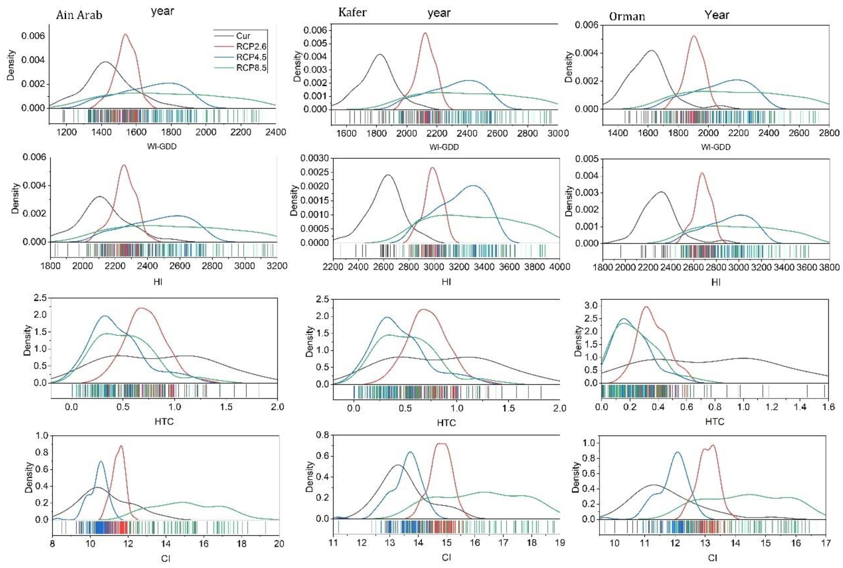
Estimates of the BVIs were conducted for three regions, namely Ain Arab, Kafer, and Orman, for a baseline period of 31 years from 1984 to 2014, as well as for the three RCPs - RCP2.6, RCP4.5, and RCP8.5 - over 86 years from 2015 to 2100. The study found that the highest increase in GDD under RCP2.6 compared to the baseline was estimated in Orman (18.5%), followed by Kfer (17.6%) and Ain Arab (6.6%). This same trend was observed under RCP4.5 and RCP8.5 in all three regions, with the highest magnitudes being 29.5%, 28%, and 16.1% under RCP4.5, and 35.8%, 33.6%, and 22.9% under RCP8.5, respectively (Table 3). In addition, the coefficient of variation (CV) varied across the three regions and different scenarios, with the lowest CV being 3.8% under RCP2.6 in Ain Arab and the highest being 16.9% under RCP8.5, also in Ain Arab. For Al Kfer, the CV ranged from 3.0% under RCP2.6 to 12.7% under RCP8.5, while for Orman, it ranged from 3.3% under RCP2.6 to 14.3% under RCP8.5. Regarding the change in HI, the study estimated that the highest increase under RCP2.6 compared to baseline was in Orman (16.2%), followed by Kfer (14.3%) and Ain Arab (5.9%). This same trend was observed under RCP4.5 and RCP8.5, with magnitudes of 25.9%, 22.5%, and 15.8% under RCP4.5, and 30.8%, 26.6%, and 21.0% under RCP8.5, respectively (Table 3). The coefficient of variation (CV) varied across the regions and scenarios, ranging from 2.4% to 12.7% in Kfer, from 2.8% to 11.3% in Orman, and from 3.2% to 12.7% in Ain Arab. Moreover, the study estimated that the highest decrease in HTC under RCP2.6 compared to baseline was in Orman (-51.9%), followed by Kfer (-18.0%) and Ain Arab (-14.5%). This same trend was also observed under RCP4.5 and RCP8.5, with magnitudes of -71.2%, -47.4%, and -46.9% under RCP4.5, and -67.7%, -41.7%, and -38.3% under RCP8.5, respectively (Table X). The CV varied across the regions and scenarios, ranging from 28.7% to 64.2% in Orman, from 31.3% to 55.3% in Kfer, and from 27.0% to 58.8% in Ain Arab. Finally, the study estimated that the highest increase in CI under RCP2.6 compared to baseline was in Orman (11.5%), followed by Kfer (9.4%) and Ain Arab (6.0%). The same trend was observed under RCP4.5, with values of 1.6%, 0.4%, and -3.9% in Orman, Kfer, and Ain Arab, respectively. Under RCP8.5, however, the highest increase was estimated in Ain Arab (39.1%), followed by Orman (22.2%) and Kfer (19.9%). The coefficient of variation (CV) varied from the lowest 2.8% under RCP2.6 to the highest 11.4% under RCP8.5, and 4.7% under RCP4.5 in Ain Arab, whereas in Kfer, CV varied from 2.5% under RCP2.6 to the highest 9.0% under RCP8.5, and 4.0% under RCP4.5 and in Orman, the CV varied from lowest 2.5% under RCP2.6 to the highest 9.1% under RCP8.5, and 4.3% under RCP4.5 (data not shown).
Figure 3.
Temporal evolution of BVIs values during the 1984-2014 period for specific viticultural regions in the study area.
Figure 3.
Temporal evolution of BVIs values during the 1984-2014 period for specific viticultural regions in the study area.
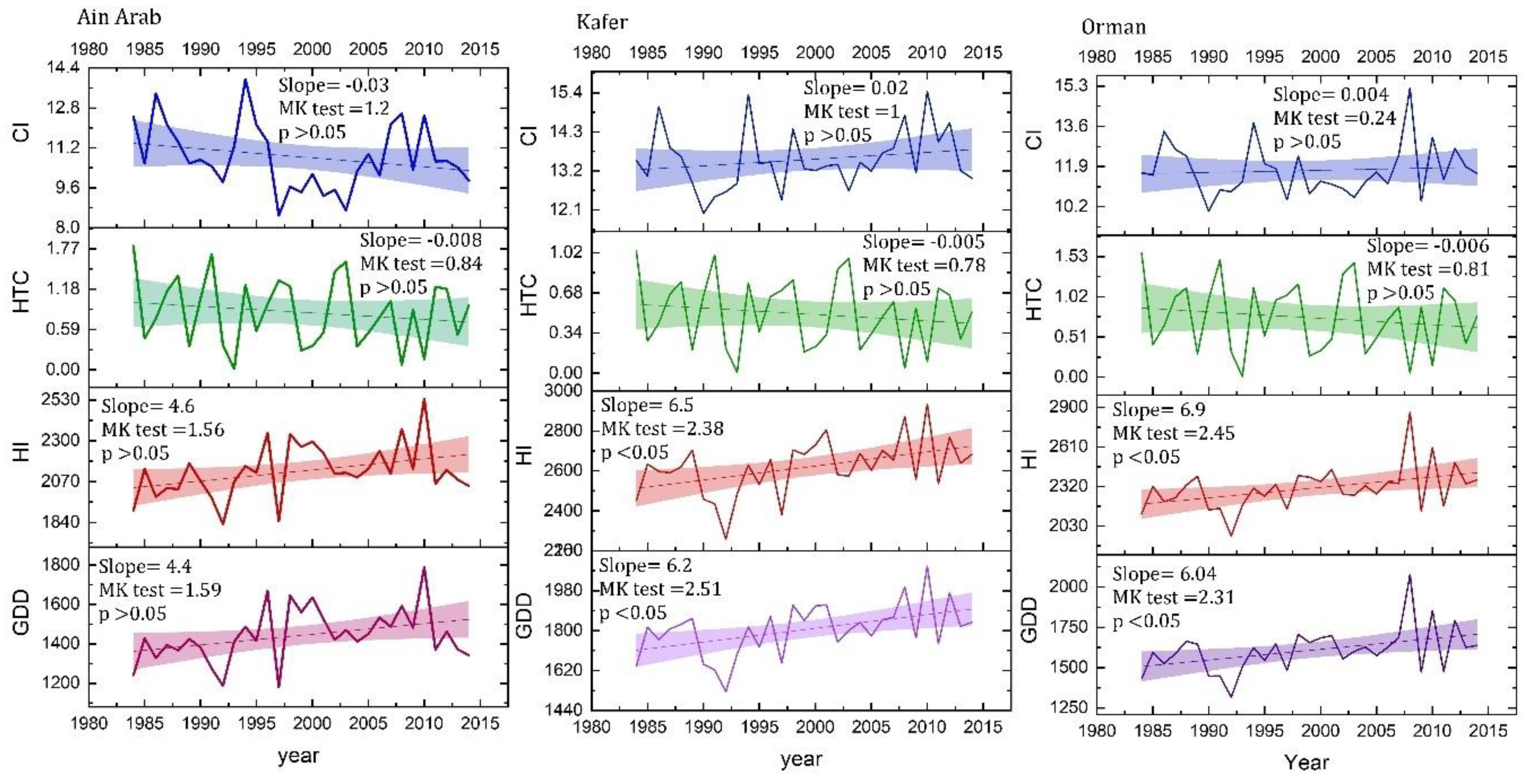
Figure 4.
The kernel smoothed probability density function of the temporal distribution of BVI values under projected climate change compared to the current climate for specific viticultural regions in the study area.
Figure 4.
The kernel smoothed probability density function of the temporal distribution of BVI values under projected climate change compared to the current climate for specific viticultural regions in the study area.
3.3. Delineation of BVIs zones under projected climate change
To assess the spatial distribution of BVIs zones at a 1 km spatial resolution, analyses were conducted using the RK method for both current climate conditions (referred to as the "1984-2014 period") and projected climate change scenarios (RCPs). Zonal statistical analysis was performed for the study area, revealing significant changes between 1984-2014 and the RCPs (Figure 5). The results indicated that under current climate conditions, the GST indicator showed that 71.7% of the study area was classified as the Hot zone (H), while the Warm (W) and Temperate (T) zones covered approximately 20% and 7.8% of the study area, respectively. However, when considering climate change scenarios, the Hot zone expanded significantly. It was projected that 91%, 96.5%, and 97.9% of the study area would be dominated by the Hot zone for RCP2.6, RCP4.5, and RCP8.5 scenarios, respectively. These areas witnessed an increase of +20.3%, +24.8%, and +26.2% compared to the current climate conditions (see Table 3). Additionally, the Warm zone is expected to shift towards the elevated areas in the central part of the study area under climate change scenarios.
Since the WI-GDD and HI provide information on the accumulation of heat during the growing season for vineyards and thus provide better information regarding the sugar potential accumulation of given varieties and climate-maturity zoning, we assessed the spatial distribution of WI-GDD and HI as given in Figure for both current climate conditions and RCPs. The results indicated that under current climate conditions, the WI-GDD showed that only 2.6% of the study area was classified as the Too Hot zone (TH), while the Hot (H) zone covered approximately 40.3% of the study area. However, when considering climate change scenarios (RCPs), the Too Hot zone expanded significantly. It projected to be that 36.5%, 60.7%, and 72.5% of the study area would be dominated by the Too Hot zone for RCP2.6, RCP4.5, and RCP8.5 scenarios, respectively. These areas witnessed an increase of +33.9%, +58.1%, and +69.6% compared to the current climate conditions (see Table 3). Moreover, the Hot zone and Moderately Warm (MW) zone are expected to shift towards the elevated areas in the central part of the study area under climate change scenarios, resulting in a decrease in their percentage distribution compared to the current climate conditions. Notably, the Moderately Cold (MC) and Warm (W) zones, which are the most important zones for viticulture cultivation, are projected to decrease these zones under climate change scenarios. The MC zone is expected to decrease by 6.3%, 8%, and 8% from the study area, while the W zone is expected to decrease by 9.4%, 3.8%, and 14.7% from the study area, for RCP2.6, RCP4.5, and RCP8.5 scenarios, respectively, compared to the current climate. The same results were obtained for HI zoned with slight changes compared to the WI-GDD (see Figure 5 and Table 4).
In terms of the spatial distribution of HTC, which determines the suitability for rainfed viticulture, the study classified the region into six classes ranging from excessively dry (ED) to excessively wet (EW) (Table 2). The results indicated that under current climate conditions, the study area can be divided into three zones: ED, D, and MD zones, covering approximately 52.8%, 34.9%, and 12.3% of the study area, respectively. The MD zone, considered the optimal region with HTC values ranging from 0.5 to 1.0 mm/°C, is expected to decrease by 7.4% in terms of coverage area under the RCP2.6 scenario. However, this zone is projected to disappear entirely under the RCP4.5 and RCP8.5 scenarios. These findings suggest that grape production based on these scenarios would only be possible with irrigation due to the unsuitability of the climate for rainfed viticulture.
The values in parentheses are the percentage of change (%) compared to current climate values.
In terms of the spatial distribution of CI, which is a significant indicator of grape and wine color and aromas, the study examined its variations under both current climate conditions and different RCPs scenarios. The findings revealed that the study area can be classified into four zones under current climate conditions: VCN, CN, TN, and WN zones, covering approximately 4.2%, 6.7%, 85.8%, and 3.3% of the study area, respectively. The WN zone is projected to expand by +50.3%, +12.3%, and +72.6% from the study area under the RCP2.6, RCP4.5, and RCP8.5 scenarios, respectively. On the other hand, the CN zone (considered the optimal region with CI values >12 and ≤ 14 C) is expected to decrease by 3.6%, 1.6%, and 5% from the study area under the RCP2.6, RCP4.5, and RCP8.5 scenarios. Furthermore, the VCN zone is anticipated to disappear under the RCP2.6 and RCP8.5 scenarios. These findings suggest that the warming projected under the RCPs will significantly impact the spatial distribution of CI, subsequently influencing the quality of grapes in terms of secondary metabolites such as aromas and polyphenols. It can also impede sugar accumulation and anthocyanins. For more details regarding the BVIs values and zones under projected climate change compared to the current climate for major viticultural regions in the study area see Table 5.
4. Discussion
Global warming and climatic change are the most deliberated matters in the last few decades due to their environmental, biological, and socio-economic consequences (IPCC, 2014). Global warming is likely to have a significant impact on agriculture and crop pro-duction (Mokhtar et al. 2020, 2021), but especially on viticultural production, because grapevines are extremely vulnerable to climate change and variability (Fraga et al. 2019; Piña-Rey et al. 2020; Alba et Al. 2021; Xyrafis et al. 2022). Climate has a significant impact on agricultural aptitude and grapevine production (Ramos et al.2008; Ponti et al. 2018; Arias et al. 2022). Climate variables (solar radiation, air temperature, relative humidity, and rainfall amounts) that have a greater influence on grape growing and Vitis vinifera grapevines production, as well as wine grape quality, have been extensively studied in the case of the grapevine in response to increasing global warming, and according to some works (e.g., Rankine, 1990; Cardell et al. 2019; Sgubin et al. 2023), the temperature is regarded as the most important climatic variable affecting grapevine growth (Jones, 2012). Grapevine composition and quality, in particular, are affected by air temperature (e.g., Coombe 1987, van Leeuwen et al. 2009), as well as wine qualities (Jackson and Lombard 1993; Jones et al. 2005), very cold temperatures can cause ripening to be delayed or even prevented, can impede the sugar accumulation and anthocyanins formation, resulting in wines with poor alcohol contents and poorly developed taste profiles (Jackson and Lombard 1993; Sadras and Moran, 2012; Clemente et al. 2022; Arias et al. 2022). Too much temperature throughout the season, on the other hand, might cause grapes to mature early in the growing season, with increased sugar formation but low acidity, resulting in an imbalanced wine (Mira de Orduna 2010). Also, temperature fluctuation effects on vineyards have been seen to modify the duration of phenological periods and growth seasons, the timing and severity of diseases, and pests, resulting in effects on the quality and quantity of grapes produced (Valori et al. 2023; Ausseil et al. 2021; Costa et al., 2019; Ponti et al. 2018; Verdugo-Vásquez et al. 2016; Sadras and Moran, 2013; Caffarra et al., 2012).
The BVIs provide valuable insights into the suitability of different grape varieties for specific regions. However, with climate change projections indicating shifts in temperature and precipitation patterns, it is crucial to examine how these changes might affect viticultural indices in the study area. The changing climate can lead to shifts in climatic zones, impacting the suitability of different grape varieties in current regions. The Climatic classification systems, such as the HI and WI-GDD, and CI use temperature thresholds to define grape-growing regions. As these temperatures-based indices change, the boundaries of climatic zones will be changed. For example, cool-climate regions may experience warmer temperatures, allowing the cultivation of grape varieties that were previously unsuitable (elevated areas in Jabal Arab). Conversely, some traditional warm-climate regions (Kafer, Hobran, and Orman) may face a decline in suitability for certain grape varieties due to increased heat stress. Previous studies have indicated a northward shift in suitable viticultural regions in Europe, regions such as Germany, England, Poland, and parts of Scandinavia and some central parts of Europe have seen an expansion in their viticultural potential due to milder temperatures and longer growing seasons (Droulia and Charalampopoulos, 2022; Nesbitt et al., 2016; Cardell et al. 2019). In contrast, the temperatures-based indices such as the WI-GDD show an upward trend under climate change in many southern European viticulture regions, higher BVIs values indicate an increase in the heat available for grape ripening this trend has been observed in regions like the Apulia region in Italy ( Gentilesco et al., 2023), Douro Valley in Portugal (Blanco-Ward et al. 2019), Lake Neuchatel in Switzerland (Comte et al. 2022), Santorini Island in Greece (Xyrafis et al. 2022).
Our study suggests that changing climate can lead to shifts in the BVIs zones in the study area to be warmer, and will experience an increase in the GDD, HI, TGS, and CI potentially leading to alterations in grape variety suitability. For instance, some traditional grape-growing regions (Kafer, Hobran, Mayamas, and Orman) may become too hot for certain grape varieties, necessitating the adoption of heat-tolerant cultivars. Furthermore, we cannot be shifted suddenly the viticultural regions with climatic change due to a variety of socio-economic issues (Mosedale et al., 2016), such as long-dated reestablishment times, market accessibility, labor availability, and others. As a result, the importance of coping with climate change in viticulture is founded on three critical factors: (1) the grapevines are planted for several decades, and new plantations may take 15–30 years to yield full outputs; thus, the cultivars chosen should be adapted to rising temperatures and decreasing precipitation; (2) regulations on production practices and varieties adapt slowly; and (3) the properties of its final product are not only the outcome of terroir, which describes the relationship between vineyards, pedology, the cultivation process, and climatic variables, but also an expression of cultural and socio-economic parameters (Resco et al. 2015). Although viticultural can adapt to the short- to medium-term effects of climate change, genetic enhancement is required to give long-term sustainable solutions to these issues (van Leeuwen et al. 2019; Delrot et al. 2020). As a result, the shifting of high-quality varieties to suitable areas for their cultivation (i.e., by their shifting to higher elevations, more than 1400 m) is possible in the future (see Recommended grapevine cultivars in Table 6 under RCP2.6).
5. Conclusions
The objective of this research was to evaluate the climatic zones for viticulture in the Jabal Arab region located in the Eastern Mediterranean. The study employed the regression-kriging (RK) method along with five bioclimatic indices. Historical and future time-series data until the end of the 21st century were analyzed. The findings indicated a rise in temperature as a result of climate change, which was already evident when comparing the historical periods of 1984-2014. This temperature increase is projected to continue in future scenarios, with varying values ranging from 0.8°C to 4.1°C depending on the considered RCPs. The bioclimatic indices used in this study revealed that under the milder and more reliable RCP-2.6 scenario, there will still be opportunities for cultivating quality vineyards, even in smaller elevated areas than the current cultivated ones. However, the RCP-8.5 and RCP-4.5 scenarios indicated increasing trends of BVIs by the end of the century in the Jabal Arab region. These results emphasize the importance of territories like Jabal Arab, which have a historical suitability for viticulture, to make prompt decisions to address climate change. This can be achieved through adjusting technical and agronomical practices to maintain competitiveness in the global grape market, especially considering the emergence of new players from regions where vineyard relocation has already begun.
It should be noted that these results do not necessarily imply a significant decline in viticulture suitability in the study area in the medium and long-term future scenarios, as adaptive strategies can be implemented, which are already being undertaken by grapevine growers in the region. In light of this, several actions can be recommended to preserve the typicity of high-quality varieties in the region, based on current knowledge and previous studies conducted in the area, such as Alsafadi et al. (2016). Key strategies include clonal selection, appropriate rootstocks, and the cultivation of late-ripening local or carefully selected non-local varieties to delay phenology stages. Training systems and late pruning can also be beneficial in delaying phenology and reducing water deficit. It is crucial to carefully assess the necessity of irrigation considering its economic, environmental, and social implications. Additionally, increasing the soil's water-holding capacity, selecting drought-resistant rootstocks, and implementing genetic enhancement is essential for achieving long-term sustainability.
Author Contributions
Conceptualization, K.A.; methodology, K.A.; software, K.A.; formal analysis, K.A.; investigation, K.A.; data curation, K.A.; writing—original draft preparation, K.A., and A.K.S.; writing—review and editing, K.A., S.B., B.B., A.A. and A.K.S.; visualization, K.A.; supervision, S.B.; funding acquisition, A.A., B.B., and S.B. All authors have read and agreed to the published version of the manuscript.
Funding
This work was supported by the National Natural Science Foundation of China (grant numbers 41971340 and 41271410), and also was supported by the Researchers Supporting Project (grant number RSP2023R296), King Saud University, Riyadh, Saudi Arabia.. We also acknowledge the funding by the German Federal Ministry of Education and Research (BMBF) in the framework of the funding measure ‘Soil as a Sustainable Resource for the Bioeconomy— BonaRes’, project BonaRes (Module A): BonaRes Center for Soil Research, subproject ‘Sustainable Subsoil Management—Soil3’(Grant 031B0151A), and partially funded by the Deutsche Forschungsgemeinschaft (DFG, German Research Foundation) under Germany’s Excellence Strategy—EXC 2070—390732324.
Data Availability Statement
The data that support the findings of this study are available upon request.
Conflicts of Interest
The authors declare no conflict of interest.
References
- Alba, V.; Gentilesco, G.; Tarricone, L. Climate Change in a Typical Apulian Region for Table Grape Production: Spatialisation of Bioclimatic Indices, Classification and Future Scenarios. Oeno One 2021, 51. [CrossRef]
- Alexandersson, H. A Homogeneity Test Applied to Precipitation Data. Journal of Climatology 1986, 6, 661–675. [CrossRef]
- Alsafadi, K.; Mohammed, S.; Habib, H.; Kiwan, S.; Hennawi, S.; Sharaf, M. An Integration of Bioclimatic, Soil, and Topographic Indicators for Viticulture Suitability Using Multi-Criteria Evaluation: A Case Study in the Western Slopes of Jabal Al Arab—Syria. Geocarto International 2020, 35, 1466–1488. [CrossRef]
- Alsafadi, K.; Mohammed, S.; Mokhtar, A.; Sharaf, M.; He, H. Fine-Resolution Precipitation Mapping over Syria Using Local Regression and Spatial Interpolation. Atmospheric Research 2021, 256. [CrossRef]
- Alsafadi, K.; Bi, S.; Abdo, H.G.; Almohamad, H.; Alatrach, B.; Srivastava, A.K.; Al-Mutiry, M.; Bal, S.K.; Chandran, M.A.S.; Mohammed, S. Modeling the Impacts of Projected Climate Change on Wheat Crop Suitability in Semi-Arid Regions Using the AHP-Based Weighted Climatic Suitability Index and CMIP6. Geoscience Letters 2023, 10. [CrossRef]
- Alsafadi, K.; Bi, S.; Bashir, B.; Sharifi, E.; Alsalman, A.; Kumar, A.; Shahid, S. High-Resolution Precipitation Modeling in Complex Terrains Using Hybrid Interpolation Techniques: Incorporating Physiographic and MODIS Cloud Cover Influences. Remote Sensing 2023, 15. [CrossRef]
- Amerine, M.A.; Winkler, A.J. Composition and Quality of Musts and Wines of California Grapes. Hilgardia 1944, 15. [CrossRef]
- Jones, G. V.; Duff, A.; Hall, A. Updated Analysis of Climate-Viticulture Structure and Suitability in the Western United States. American Journal of Enology and Viticulture 2009, 60.
- Ausseil, A.G.E.; Law, R.M.; Parker, A.K.; Teixeira, E.I.; Sood, A. Projected Wine Grape Cultivar Shifts Due to Climate Change in New Zealand. Frontiers in Plant Science 2021, 12. [CrossRef]
- Badr, G.; Hoogenboom, G.; Abouali, M.; Moyer, M.; Keller, M. Analysis of Several Bioclimatic Indices for Viticultural Zoning in the Pacific Northwest. Climate Research 2018, 76. [CrossRef]
- Blanco-Ward, D.; García Queijeiro, J.M.; Jones, G. V. Spatial Climate Variability and Viticulture in the Miño River Valley of Spain. Vitis - Journal of Grapevine Research 2007, 46. [CrossRef]
- Blanco-Ward, D.; Monteiro, A.; Lopes, M.; Borrego, C.; Silveira, C.; Viceto, C.; Rocha, A.; Ribeiro, A.; Andrade, J.; Feliciano, M.; et al. Climate Change Impact on a Wine-Producing Region Using a Dynamical Downscaling Approach: Climate Parameters, Bioclimatic Indices and Extreme Indices. International Journal of Climatology 2019, 39. [CrossRef]
- Cabré, F.; Nuñez, M. Impacts of Climate Change on Viticulture in Argentina. Regional Environmental Change 2020, 20. [CrossRef]
- Cabré, M.F.; Quénol, H.; Nuñez, M. Regional Climate Change Scenarios Applied to Viticultural Zoning in Mendoza, Argentina. International Journal of Biometeorology 2016, 60. [CrossRef]
- Caffarra, A.; Rinaldi, M.; Eccel, E.; Rossi, V.; Pertot, I. Modelling the Impact of Climate Change on the Interaction between Grapevine and Its Pests and Pathogens: European Grapevine Moth and Powdery Mildew. Agriculture, Ecosystems and Environment 2012, 148. [CrossRef]
- Cardoso, A.S.; Alonso, J.; Rodrigues, A.S.; Araújo-Paredes, C.; Mendes, S.; Valín, M.I. Agro-Ecological Terroir Units in the North West Iberian Peninsula Wine Regions. Applied Geography 2019, 107. [CrossRef]
- Clemente, N.; Santos, J.A.; Fontes, N.; Graça, A.; Gonçalves, I.; Fraga, H. Grapevine Sugar Concentration Model (GSCM): A Decision Support Tool for the Douro Superior Winemaking Region. Agronomy 2022, 12. [CrossRef]
- Costa, R.; Fraga, H.; Fonseca, A.; De Cortázar-Atauri, I.G.; Val, M.C.; Carlos, C.; Reis, S.; Santos, J.A. Grapevine Phenology of Cv. Touriga Franca and Touriga Nacional in the Douro Wine Region: Modelling and Climate Change Projections. Agronomy 2019, 9. [CrossRef]
- Coombe, B.G. Distribution of Solutes within the Developing Grape Berry in Relation to Its Morphology. American Journal of Enology and Viticulture 1987, 38. [CrossRef]
- Danielson, J.J., Gesch, D.B. Global Multi-Resolution Terrain Elevation Data 2010 (GMTED2010); 2011;
- Delrot, S.; Grimplet, J.; Carbonell-Bejerano, P.; Schwandner, A.; Bert, P.F.; Bavaresco, L.; Costa, L.D.; Di Gaspero, G.; Duchêne, E.; Hausmann, L.; et al. Genetic and Genomic Approaches for Adaptation of Grapevine to Climate Change. In Genomic Designing of Climate-Smart Fruit Crops; 2020.
- Fraga, H.; Malheiro, A.C.; Moutinho-Pereira, J.; Cardoso, R.M.; Soares, P.M.M.; Cancela, J.J.; Pinto, J.G.; Santos, J.A. Integrated Analysis of Climate, Soil, Topography and Vegetative Growth in Iberian Viticultural Regions. PLoS ONE 2014, 9. [CrossRef]
- Fraga, H.; Pinto, J.G.; Santos, J.A. Climate Change Projections for Chilling and Heat Forcing Conditions in European Vineyards and Olive Orchards: A Multi-Model Assessment. Climatic Change 2019, 152. [CrossRef]
- Gaál, M.; Moriondo, M.; Bindi, M. Modelling the Impact of Climate Change on the Hungarian Wine Regions Using Random Forest. Applied Ecology and Environmental Research 2012, 10. [CrossRef]
- Gebrechorkos, S.H.; Hülsmann, S.; Bernhofer, C. Statistically Downscaled Climate Dataset for East Africa. Scientific Data 2019, 6. [CrossRef]
- Goovaerts, P. Geostatistical Approaches for Incorporating Elevation into the Spatial Interpolation of Rainfall. Journal of Hydrology 2000, 228, 113–129. [CrossRef]
- Hall, A.; Blackman, J. Modelling Within-Region Spatiotemporal Variability in Grapevine Phenology with High Resolution Temperature Data. In Proceedings of the Oeno One; 2019; Vol. 53.
- Hall, A.; Jones, G. V. Spatial Analysis of Climate in Winegrape-Growing Regions in Australia. Australian Journal of Grape and Wine Research 2010, 16. [CrossRef]
- Hengl, T.; Heuvelink, G.B.M.; Rossiter, D.G. About Regression-Kriging: From Equations to Case Studies. Computers and Geosciences 2007, 33, 1301–1315. [CrossRef]
- Hofmann, M.; Volosciuk, C.; Dubrovský, M.; Maraun, D.; Schultz, H.R. Downscaling of Climate Change Scenarios for a High-Resolution, Site-Specific Assessment of Drought Stress Risk for Two Viticultural Regions with Heterogeneous Landscapes. Earth System Dynamics 2022, 13. [CrossRef]
- IPCC Climate Change 2014: Synthesis Report. Contribution of Working Groups I, II and III to the Fifth Assessment Report of the Intergovernmental Panel on Climate Change; 2014;
- Jackson, D.I.; Lombard, P.B. Environmental and Management Practices Affecting Grape Composition and Wine Quality - A Review. American Journal of Enology and Viticulture 1993, 44. [CrossRef]
- Jarvis, C.; Barlow, E.; Darbyshire, R.; Eckard, R.; Goodwin, I. Relationship between Viticultural Climatic Indices and Grape Maturity in Australia. International Journal of Biometeorology 2017, 61. [CrossRef]
- Jones, G. V.; White, M.A.; Cooper, O.R.; Storchmann, K. Climate Change and Global Wine Quality. Climatic Change 2005, 73. [CrossRef]
- Jones, G. V. Climate, Grapes, and Wine: Structure and Suitability in a Changing Climate. In Proceedings of the Acta Horticulturae; 2012; Vol. 931.
- Jones, G. V.; Duff, A.A.; Hall, A.; Myers, J.W. Spatial Analysis of Climate in Winegrape Growing Regions in the Western United States. American Journal of Enology and Viticulture 2010, 61. [CrossRef]
- Jones, N.K. An Investigation of Trends in Viticultural Climatic Indices in Southern Quebec, a Cool Climate Wine Region. Journal of Wine Research 2018, 29. [CrossRef]
- Anderson, J.D.; Jones, G. V; Tait, A.; Hall, A.; Trought, M.C.T. Analysis of Viticulture Region Climate Structure and Suitability in New Zealand. OENO One 2012, 46, 149–165. [CrossRef]
- Köse, B. Phenology and Ripening of Vitis Vinifera L. and Vitis Labrusca L. Varieties in the Maritime Climate of Samsun in Turkey’s Black Sea Region. South African Journal of Enology and Viticulture 2014, 35. [CrossRef]
- Kliewer, W.M. Berry Composition of Vitis Vinifera Cultivars as Influenced by Photo- and Nycto-Temperatures During Maturation. Journal of the American Society for Horticultural Science 1973, 98, 153–159. [CrossRef]
- Le Roux, R.; de Rességuier, L.; Corpetti, T.; Jégou, N.; Madelin, M.; van Leeuwen, C.; Quénol, H. Comparison of Two Fine Scale Spatial Models for Mapping Temperatures inside Winegrowing Areas. Agricultural and Forest Meteorology 2017, 247. [CrossRef]
- Meenu, R.; Rehana, S.; Mujumdar, P.P. Assessment of Hydrologic Impacts of Climate Change in Tunga-Bhadra River Basin, India with HEC-HMS and SDSM. Hydrological Processes 2013, 27. [CrossRef]
- Mesterházy, I.; Mészáros, R.; Pongrácz, R. The Effects of Climate Change on Grape Production in Hungary. Idojaras 2014, 118.
- Mira de Orduña, R. Climate Change Associated Effects on Grape and Wine Quality and Production. Food Research International 2010, 43. [CrossRef]
- Mohammed, S.; Alsafadi, K.; Talukdar, S.; Kiwan, S.; Hennawi, S.; Alshihabi, O.; Sharaf, M.; Harsanyie, E. Estimation of Soil Erosion Risk in Southern Part of Syria by Using RUSLE Integrating Geo Informatics Approach. Remote Sensing Applications: Society and Environment 2020, 20, 100375. [CrossRef]
- Mohammed, S.; Alsafadi, K.; Hennawi, S.; Mousavi, S.M.N.; Kamal-Eddin, F.B.; Harsanyie, E. Effects of Long-Term Agricultural Activities on the Availability of Heavy Metals in Syrian Soil: A Case Study in Southern Syria. Journal of the Saudi Society of Agricultural Sciences 2021. [CrossRef]
- Mohammed, S.; Alsafadi, K.; Enaruvbe, G.O.; Harsányi, E. Assessment of Soil Micronutrient Level for Vineyard Production in Southern Syria. Modeling Earth Systems and Environment 2021. [CrossRef]
- Mokhtar, A.; Elbeltagi, A.; Maroufpoor, S.; Azad, N.; He, H.; Alsafadi, K.; Gyasi-Agyei, Y.; He, W. Estimation of the Rice Water Footprint Based on Machine Learning Algorithms. Computers and Electronics in Agriculture 2021, 191, 106501. [CrossRef]
- Mokhtar, A.; He, H.; Alsafadi, K.; Li, Y.; Zhao, H.; Keo, S.; Bai, C.; Abuarab, M.; Zhang, C.; Elbagoury, K.; et al. Evapotranspiration as a Response to Climate Variability and Ecosystem Changes in Southwest, China. Environmental Earth Sciences 2020, 79, 312. [CrossRef]
- Montes, C.; Perez-Quezada, J.F.; Peña-Neira, A.; Tonietto, J. Climatic Potential for Viticulture in Central Chile. Australian Journal of Grape and Wine Research 2012, 18. [CrossRef]
- Moral, F.J.; Rebollo, F.J.; Paniagua, L.L.; García, A. Climatic Spatial Variability in Extremadura (Spain) Based on Viticultural Bioclimatic Indices. International Journal of Biometeorology 2014, 58. [CrossRef]
- Morari, F.; Castrignanò, A.; Pagliarin, C. Application of Multivariate Geostatistics in Delineating Management Zones within a Gravelly Vineyard Using Geo-Electrical Sensors. Computers and Electronics in Agriculture 2009, 68. [CrossRef]
- Morin, G.; Roux, R. Le; Lemasle, P.G.; Quénol, H. Mapping Bioclimatic Indices by Downscaling Modis Land Surface Temperature: Case Study of the Saint-Emilion Area. Remote Sensing 2021, 13. [CrossRef]
- Mosedale, J.R.; Abernethy, K.E.; Smart, R.E.; Wilson, R.J.; Maclean, I.M.D. Climate Change Impacts and Adaptive Strategies: Lessons from the Grapevine. Global Change Biology 2016, 22. [CrossRef]
- Odeh, I.O.A.; McBratney, A.B.; Chittleborough, D.J. Further Results on Prediction of Soil Properties from Terrain Attributes: Heterotopic Cokriging and Regression-Kriging. Geoderma 1995, 67. [CrossRef]
- Omazić, B.; Telišman Prtenjak, M.; Prša, I.; Belušić Vozila, A.; Vučetić, V.; Karoglan, M.; Karoglan Kontić, J.; Prša, Ž.; Anić, M.; Šimon, S.; et al. Climate Change Impacts on Viticulture in Croatia: Viticultural Zoning and Future Potential. International Journal of Climatology 2020, 40. [CrossRef]
- Patriche, C.V.; Irimia, L.M. Mapping the Impact of Recent Climate Change on Viticultural Potential in Romania. Theoretical and Applied Climatology 2022, 148. [CrossRef]
- Piña-Rey, A.; González-Fernández, E.; Fernández-González, M.; Lorenzo, M.N.; Rodríguez-Rajo, F.J. Climate Change Impacts Assessment on Wine-Growing Bioclimatic Transition Areas. Agriculture (Switzerland) 2020, 10. [CrossRef]
- Ponti, L.; Gutierrez, A.P.; Boggia, A.; Neteler, M. Analysis of Grape Production in the Face of Climate Change. Climate 2018, 6. [CrossRef]
- Ramos, M.C.; Jones, G. V.; Martínez-Casasnovas, J.A. Structure and Trends in Climate Parameters Affecting Winegrape Production in Northeast Spain. Climate Research 2008, 38. [CrossRef]
- Huggett, J.M. Geology and Wine: A Review. Proceedings of the Geologists’ Association 2006, 117.
- Resco, P.; Iglesias, A.; Bardají, I.; Sotés, V. Exploring Adaptation Choices for Grapevine Regions in Spain. Regional Environmental Change 2016, 16. [CrossRef]
- Sadras, V.O.; Moran, M.A. Elevated Temperature Decouples Anthocyanins and Sugars in Berries of Shiraz and Cabernet Franc. Australian Journal of Grape and Wine Research 2012, 18. [CrossRef]
- Sadras, V.O.; Moran, M.A. Nonlinear Effects of Elevated Temperature on Grapevine Phenology. Agricultural and Forest Meteorology 2013, 173. [CrossRef]
- Santos, J.A.; Malheiro, A.C.; Karremann, M.K.; Pinto, J.G. Statistical Modelling of Grapevine Yield in the Port Wine Region under Present and Future Climate Conditions. International Journal of Biometeorology 2011, 55. [CrossRef]
- Santos, J.; Malheiro, A.; Pinto, J.; Jones, G. Macroclimate and Viticultural Zoning in Europe: Observed Trends and Atmospheric Forcing. Clim. Res. 2012, 51, 89–103. [CrossRef]
- Sgubin, G.; Swingedouw, D.; Mignot, J.; Gambetta, G. A.; Bois, B.; Loukos, H.; Noël, T.; Pieri, P.; de Cortázar-Atauri, I.; Ollat, N.; et al. Non-Linear Loss of Suitable Wine Regions over Europe in Response to Increasing Global Warming. Glob. Chang. Biol., 2023, 29 (3), 808–826. [CrossRef]
- Štěpánek, P.; Zahradníček, P.; Skalák, P. Data Quality Control and Homogenization of Air Temperature and Precipitation Series in the Area of the Czech Republic in the Period 1961–2007. Adv. Sci. Res., 2009, 3 (1), 23–26. [CrossRef]
- Sturman, A.; Zawar-Reza, P.; Soltanzadeh, I.; Katurji, M.; Bonnardot, V.; Parker, A. K.; Trought, M. C. T.; Quénol, H.; Le Roux, R.; Gendig, E.; et al. The Application of High-Resolution Atmospheric Modelling to Weather and Climate Variability in Vineyard Regions. Oeno One, 2017, 51 (2). [CrossRef]
- Tavakol-Davani, H.; Nasseri, M.; Zahraie, B. Improved Statistical Downscaling of Daily Precipitation Using SDSM Platform and Data-Mining Methods. Int. J. Climatol., 2013, 33 (11). [CrossRef]
- Tonietto, J.; Carbonneau, A. A Multicriteria Climatic Classification System for Grape-Growing Regions Worldwide. Agric. For. Meteorol., 2004, 124 (1–2). [CrossRef]
- Valori, R.; Costa, C.; Figorilli, S.; Ortenzi, L.; Manganiello, R.; Ciccoritti, R.; Cecchini, F.; Morassut, M.; Bevilacqua, N.; Colatosti, G.; et al. Advanced Forecasting Modeling to Early Predict Powdery Mildew First Appearance in Different Vines Cultivars. Sustain., 2023, 15 (3). [CrossRef]
- Van Leeuwen, C.; Tregoat, O.; Choné, X.; Bois, B.; Pernet, D.; Gaudillére, J. P. Vine Water Status Is a Key Factor in Grape Ripening and Vintage Quality for Red Bordeaux Wine. How Can It Be Assessed for Vineyard Management Purposes? J. Int. des Sci. la Vigne du Vin, 2009, 43 (3). [CrossRef]
- Verdugo-Vásquez, N.; Acevedo-Opazo, C.; Valdés-Gómez, H.; Araya-Alman, M.; Ingram, B.; García de Cortázar-Atauri, I.; Tisseyre, B. Spatial Variability of Phenology in Two Irrigated Grapevine Cultivar Growing under Semi-Arid Conditions. Precis. Agric., 2016, 17 (2). [CrossRef]
- Vivier, M. A.; Pretorius, I. S. Genetically Tailored Grapevines for the Wine Industry. Trends in Biotechnology. 2002. [CrossRef]
- Vukovic, A.; Vujadinovic, M.; Ruml, M.; Rankovic-Vasic, Z.; Przic, Z.; Beslic, Z.; Matijasevic, S.; Vujovic, D.; Todic, S.; Markovic, N.; et al. Implementation of Climate Change Science in Viticulture Sustainable Development Planning in Serbia. In E3S Web of Conferences; 2018; Vol. 50. [CrossRef]
- Wilby, R. L.; Dawson, C. W.; Barrow, E. M. SDSM - A Decision Support Tool for the Assessment of Regional Climate Change Impacts. Environ. Model. Softw., 2002, 17 (2). [CrossRef]
- Xyrafis, E. G.; Fraga, H.; Nakas, C. T.; Koundouras, S. A Study on the Effects of Climate Change on Viticulture on Santorini Island. Oeno One, 2022, 56 (1). [CrossRef]
- Zorer, R.; Rocchini, D.; Metz, M.; Delucchi, L.; Zottele, F.; Meggio, F.; Neteler, M. Daily MODIS Land Surface Temperature Data for the Analysis of the Heat Requirements of Grapevine Varieties. IEEE Trans. Geosci. Remote Sens., 2013, 51 (4). [CrossRef]
- Droulia, F.; Charalampopoulos, I. A Review on the Observed Climate Change in Europe and Its Impacts on Viticulture. Atmosphere. 2022. [CrossRef]
- Nesbitt, A.; Kemp, B.; Steele, C.; Lovett, A.; Dorling, S. Impact of Recent Climate Change and Weather Variability on the Viability of UK Viticulture - Combining Weather and Climate Records with Producers’ Perspectives. Aust. J. Grape Wine Res., 2016, 22 (2). [CrossRef]
- Cardell, M. F.; Amengual, A.; Romero, R. Future Effects of Climate Change on the Suitability of Wine Grape Production across Europe. Reg. Environ. Chang., 2019, 19 (8). [CrossRef]
- Blanco-Ward, D.; Ribeiro, A.; Barreales, D.; Castro, J.; Verdial, J.; Feliciano, M.; Viceto, C.; Rocha, A.; Carlos, C.; Silveira, C.; et al. Climate Change Potential Effects on Grapevine Bioclimatic Indices: A Case Study for the Portuguese Demarcated Douro Region (Portugal). BIO Web Conf., 2019, 12. [CrossRef]
- Gentilesco, G.; Coletta, A.; Tarricone, L.; Alba, V. Bioclimatic Characterization Relating to Temperature and Subsequent Future Scenarios of Vine Growing across the Apulia Region in Southern Italy. Agriculture, 2023, 13 (3). [CrossRef]
- Comte, V.; Schneider, L.; Calanca, P.; Rebetez, M. Effects of Climate Change on Bioclimatic Indices in Vineyards along Lake Neuchatel, Switzerland. Theor. Appl. Climatol., 2022, 147 (1–2). [CrossRef]
- Van Leeuwen, C.; Destrac-Irvine, A.; Dubernet, M.; Duchêne, E.; Gowdy, M.; Marguerit, E.; Pieri, P.; Parker, A.; De Rességuier, L.; Ollat, N. An Update on the Impact of Climate Change in Viticulture and Potential Adaptations. Agronomy. 2019. [CrossRef]
- Arias, L. A.; Berli, F.; Fontana, A.; Bottini, R.; Piccoli, P. Climate Change Effects on Grapevine Physiology and Biochemistry: Benefits and Challenges of High Altitude as an Adaptation Strategy. Frontiers in Plant Science. 2022. [CrossRef]
- OIV (2012). Guidelines for vitiviniculture zoning. Methodologies on a soil and climate level. Resolution OIV-VITI 423-2012 REV1. (Izmir).
- Le Roux R, Katurji MM, Zawar-Reza P, de Resseguier L, Sturman AP, van Leeuwen C, Parker A, Trought M, Quenol H (2016). A fine scale approach to map bioclimatic indices using and comparing dynamical and geostatistical methods. Willamette Valley, OR, USA: 11th International Terroir Congress. 10/07/2016-14/07/2016.
- Jones, G.V. (2006). Climate and Terroir: Impacts of Climate Variability and Change on Win”. InFine Wine and Terroir - The Geoscience Perspective. Macqueen, R.W., and Meinert, L.D., (eds.), Geoscience Canada Reprint Series Number 9, Geological Association of Canada, St. John's,Newfoundland, 247 pages.
- Huglin, P. (1978). Nouveau mode d’évaluation des possibilités héliothermiques d’un milieu viticole. In Proceedings of the Symposium International sur l’ecologie de la Vigne (pp. 89–98). Constança: Ministre de l’Agriculture et de l’Industrie Alimentaire.
- Branas J, Bernon G, Levadoux L. 1946. Elements de viticultura generale. Bordeaux (France): Imp. Dehan.
- Alsafadi, K. J. (2016). Climate and its impact on cultivation of apple and grapes crops in Alswuydaa Governorate-Syria (unpublished master’s thesis in Arabic). Alexandria University, Alexandria, Egypt.
Figure 1.
(a) Study area, spatial distribution of stations location, annual precipitation (mm.) (Alsafadi et al. 2023b), and studied viticultural regions, (b) seasonal cycles of temperature and precipitation in the study area.
Figure 1.
(a) Study area, spatial distribution of stations location, annual precipitation (mm.) (Alsafadi et al. 2023b), and studied viticultural regions, (b) seasonal cycles of temperature and precipitation in the study area.
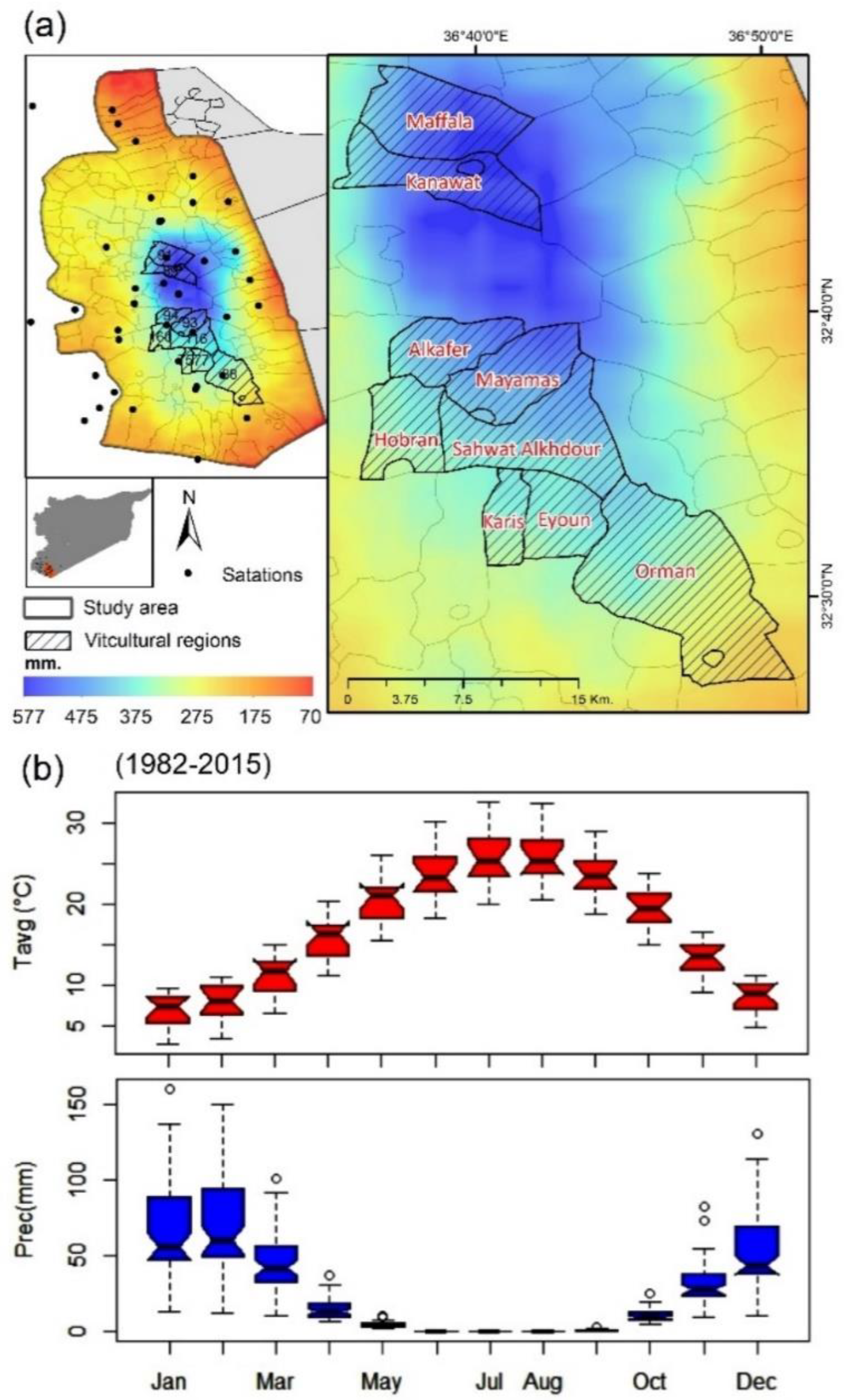
Figure 5.
Spatial distribution of BVIs zones under current climate and projected climate change for three RCPs. under sustainable development (RCP2.6), modest mitigation (RCP4.5), and unabated climate change (RCP8.5).
Figure 5.
Spatial distribution of BVIs zones under current climate and projected climate change for three RCPs. under sustainable development (RCP2.6), modest mitigation (RCP4.5), and unabated climate change (RCP8.5).
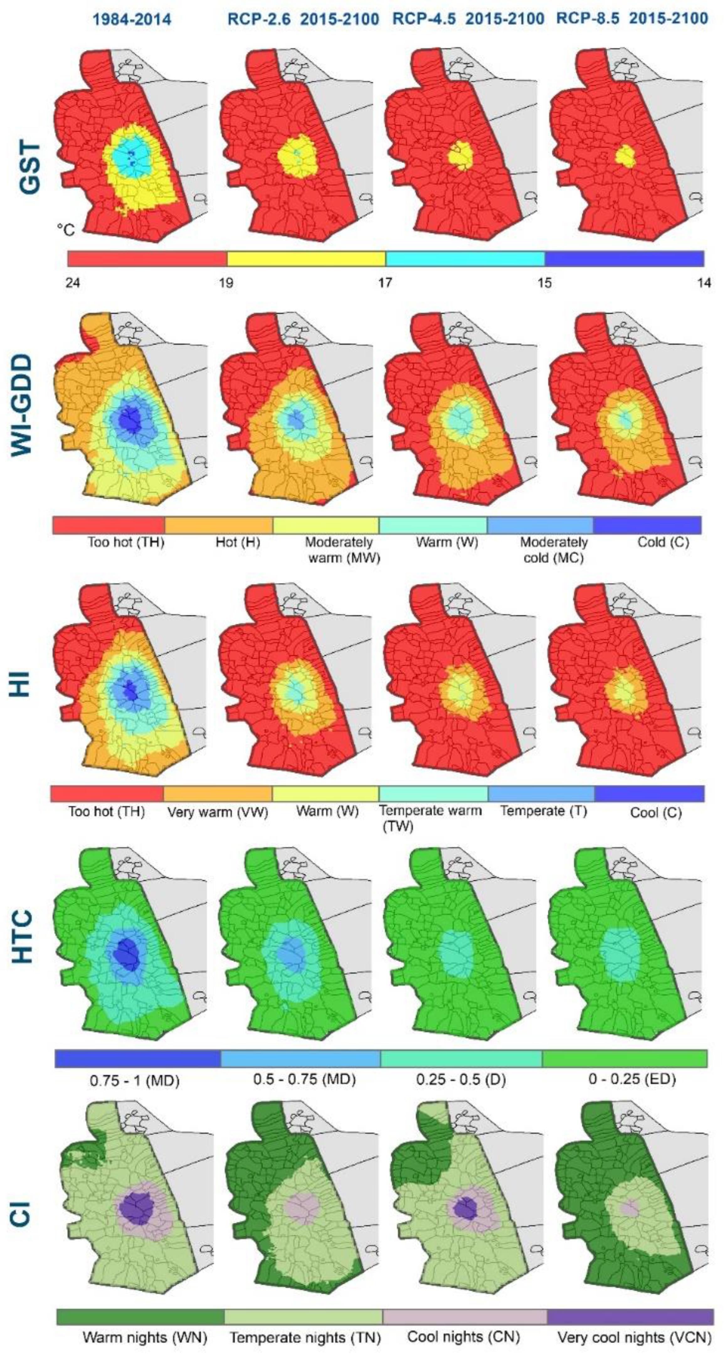
Table 1.
Observed data used in this study.
| Variable | Data type | Number of station/ point |
Temporal scale |
Reference period | Source |
| Precipitation (mm) | Rain gauge and climatic stations |
57 | Monthly | 1984 - 2014 | SMA, SMOAAR, and JMD |
| Temperature(°C) | Climatic stations | 15 | Daily | 1984 - 2014 | SMA, SMOAAR, and JMD |
| Temperature (°C) | Gridded data | 9 | Daily | 1984 - 2014 | NASA Power Data release 8.0.1 https://power.larc.nasa.gov |
Table 3.
The percentage change in GDD (Growing Degree Days), HI (Huglin Heliothermal Index), HTC (Hydrothermal Coefficient), and CI (Cool Night Index) for future scenarios spanning from 2015 to 2100 under RCP2.6, 4.5, and 8.5, in comparison to the baseline period of 1984-2014.
Table 3.
The percentage change in GDD (Growing Degree Days), HI (Huglin Heliothermal Index), HTC (Hydrothermal Coefficient), and CI (Cool Night Index) for future scenarios spanning from 2015 to 2100 under RCP2.6, 4.5, and 8.5, in comparison to the baseline period of 1984-2014.
| Regions | RCPs | GDD | HI | HTC | CI |
|---|---|---|---|---|---|
| RCP2.6 | 6.6 | 5.9 | -14.5 | 6.0 | |
| Ain Arab | RCP4.5 | 16.1 | 15.8 | -46.9 | -3.9 |
| RCP8.5 | 22.9 | 21.0 | -38.3 | 39.1 | |
| Kfer | RCP2.6 | 17.6 | 14.3 | -18.0 | 9.4 |
| RCP4.5 | 28.0 | 22.5 | -47.4 | 0.4 | |
| RCP8.5 | 33.6 | 26.6 | -41.7 | 19.9 | |
| Orman | RCP2.6 | 18.5 | 16.2 | -51.9 | 11.5 |
| RCP4.5 | 29.5 | 25.9 | -71.2 | 1.6 | |
| RCP8.5 | 35.8 | 30.8 | -67.7 | 22.2 |
Table 4.
Changes in percentage area (%) per zone of the BVI under projected climate change (2015–2100) and three RCPs compared to the current climate (1984–2014).
Table 4.
Changes in percentage area (%) per zone of the BVI under projected climate change (2015–2100) and three RCPs compared to the current climate (1984–2014).
| BVI | Zone | 1984-2014 | 2015-2100 | ||
| RCP2.6 | RCP4.5 | RCP.8.5 | |||
| GST | C | 0.2 | 0 (-0.2) | 0 (-0.2) | 0 (-0.2) |
| T | 7.8 | 0.3 (-7.5) | 0 (-7.8) | 0 (-7.8) | |
| W | 20.3 | 7.7 | 3.5 | 2.1 | |
| H | 71.7 | 92 (+20.3) | 96.5 (+24.8) | 97.9 (+26.2) | |
| WI-GDD | C | 2.9 | 0 (–2.9) | 0 (–2.9) | 0 (–2.9) |
| MC | 8 | 1.7 (–6.3) | 0 (–8) | 0 (–8) | |
| W | 15.8 | 6.4 (–9.4) | 3.8 (–12) | 1.1 (–14.7) | |
| MW | 30.3 | 11.8 (–18.5) | 7 (–23.3) | 5.2 (–25.1) | |
| H | 40.3 | 43.6 (+3.3) | 28.5 (–11.8) | 21.2 (–19.1) | |
| TH | 2.6 | 36.5 (+33.9) | 60.7 (+58.1) | 72.5 (+69.6) | |
| HI | C | 1.3 | 0 (–1.3) | 0 (–1.3) | 0 (–1.3) |
| T | 7.2 | 0 (–7.2) | 0 (–7.2) | 0 (–7.2) | |
| TW | 13.3 | 2.3 (–11) | 0.2 (–13.1) | 0 (–13.3) | |
| W | 21.3 | 7.2 (–14.1) | 4.1 (–17.2) | 2.5 (–18.8) | |
| VW | 26.5 | 13.8 (–12.7) | 8.5 (–18) | 7.3 (–19.2) | |
| TH | 30.4 | 76.7 (+46.3) | 87.2 (+56.8) | 90.2 (+59.8) | |
| HTC | ED | 52.8 | 75.5 (+22.7) | 91.3 (+38.5) | 88.9 (+36.1) |
| D | 34.9 | 19.6 (–15.3) | 8.7 (–26.2) | 11.1 (–23.8) | |
| MD | 12.3 | 4.9 (–7.4) | 0 (–12.3) | 0 (–12.3) | |
| CI | VCN | 4.2 | 0 (–4.2) | 2.2 (–2) | 0 (–4.2) |
| CN | 6.7 | 3.1 (–3.6) | 5.1 (–1.6) | 1.7 (–5) | |
| TN | 85.8 | 43.3 (–42.5) | 77.1 (–8.7) | 22.4 (–63.4) | |
| WN | 3.3 | 53.6 (+50.3) | 15.6 (+12.3) | 75.9 (+72.6) | |
Table 5.
Changes in mean BVIs values and zones under projected climate change compared to the current climate for major viticultural regions in the study area.
Table 5.
Changes in mean BVIs values and zones under projected climate change compared to the current climate for major viticultural regions in the study area.
| Scenario | region | W-GDD | HI | HTC | CI | ||||
| Mean | zone | Mean | zone | Mean | zone | Mean | zone | ||
|
Baseline 1982-2014 |
Alkars | 1826.9 | W | 2368.9 | TW | 0.46 | D | 14.6 | TN |
| Euyun | 1784.4 | W | 2318.8 | TW | 0.475 | D | 14.4 | TN | |
| Orman | 1859.4 | W | 2408.6 | W | 0.375 | D | 14.7 | TN | |
| Qanawat | 1626.5 | MC | 2140.9 | TW | 0.702 | MD | 12.7 | CN | |
| Mafeila | 1809.5 | W | 2289.3 | TW | 0.605 | MD | 14.2 | TN | |
| Mayamas | 1493.3 | MC | 1999.6 | T | 0.73 | MD | 12.1 | CN | |
| Kafer | 1631.6 | MC | 2137.7 | TW | 0.626 | MD | 12.8 | CN | |
| Sahwat Kh | 1657.6 | MC | 2183.5 | TW | 0.573 | MD | 13.3 | CN | |
| Hobran | 1855.4 | W | 2413 | W | 0.45 | D | 14.5 | TN | |
|
RCP26 2015-2100 |
Alkars | 2206.3 | MW | 2947.6 | VW | 0.325 | D | 16.6 | TN |
| Euyun | 2159 | MW | 2900.6 | VW | 0.331 | D | 16.4 | TN | |
| Orman | 2244 | H | 2997.1 | VW | 0.252 | D | 16.6 | TN | |
| Qanawat | 1995 | MW | 2693.1 | W | 0.50 | MD | 14.6 | TN | |
| Mafeila | 2191.4 | MW | 2843.7 | VW | 0.440 | D | 16.1 | TN | |
| Mayamas | 1852.6 | W | 2546.2 | W | 0.522 | MD | 14.1 | TN | |
| Kafer | 1989.5 | MW | 2694.8 | W | 0.452 | D | 14.9 | TN | |
| Sahwat Kh | 2023.2 | MW | 2754.2 | VW | 0.407 | D | 15.4 | TN | |
| Hobran | 2242.2 | H | 2980.9 | VW | 0.324 | D | 16.6 | TN | |
|
RCP45 2015-2100 |
Alkars | 2407.7 | H | 3142.2 | TH | 0.191 | ED | 15.4 | TN |
| Euyun | 2361.4 | H | 3095.2 | TH | 0.195 | ED | 15.1 | TN | |
| Orman | 2448 | H | 3191.7 | TH | 0.142 | ED | 15.4 | TN | |
| Qanawat | 2166.7 | MW | 2884.8 | VW | 0.307 | D | 13.5 | CN | |
| Mafeila | 2382.6 | H | 3036.5 | TH | 0.278 | D | 15 | TN | |
| Mayamas | 2013 | MW | 2740.6 | VW | 0.331 | D | 12.9 | CN | |
| Kafer | 2163.1 | MW | 2887.5 | VW | 0.279 | D | 13.6 | CN | |
| Sahwat Kh | 2211.3 | MW | 2948.3 | VW | 0.250 | D | 14.1 | TN | |
| Hobran | 2434.1 | H | 3173.2 | TH | 0.195 | ED | 15.3 | TN | |
|
RCP85 2015-2100 |
Alkars | 2551.5 | H | 3223.6 | TH | 0.219 | ED | 17.8 | TN |
| Euyun | 2506.6 | H | 3181.4 | TH | 0.223 | ED | 17.6 | TN | |
| Orman | 2596.5 | H | 3284.4 | TH | 0.162 | ED | 17.85 | TN | |
| Qanawat | 2320.7 | H | 2971.6 | VW | 0.352 | D | 15.7 | TN | |
| Mafeila | 2537.2 | H | 3123.1 | TH | 0.318 | D | 17.3 | TN | |
| Mayamas | 2168 | MW | 2823.2 | VW | 0.365 | D | 15.4 | TN | |
| Kafer | 2309.3 | H | 2964.4 | VW | 0.3123 | D | 16.2 | TN | |
| Sahwat Kh | 2360.3 | H | 3032.4 | TH | 0.278 | D | 16.7 | TN | |
| Hobran | 2577.6 | H | 3245.9 | TH | 0.220 | ED | 18 | WN | |
Table 6.
Recommended grapevine cultivars based on climate-maturity zoning under baseline climate and scenario of sustainable development (RCP2.6) for major viticultural regions in the study area according to Jones (2006) classification.
Table 6.
Recommended grapevine cultivars based on climate-maturity zoning under baseline climate and scenario of sustainable development (RCP2.6) for major viticultural regions in the study area according to Jones (2006) classification.
|
Baseline and scenario |
region | TGS (°C) |
Recommended grapevine cultivars based on climate-maturity zoning |
|
| range | zone | |||
|
Baseline 1982-2014 |
Alkars | 17.6–18.6 | W | Cabernet Franc, Tempranillo, Dolcetto, Merlot, Viognier Syrah, and Table grapes |
| Euyun | 17.8–18.4 | W | ||
| Mayamas | 15.4–17 | T | Pinot Noir, Chardonay, Sauvignon Blanc, and Semillon | |
| Qanawat | 14.9–19.8 | T–W | Chardonnay, Sauvignon Blanc, Semillon, Cabernet Franc, Tempranillo, Dolcetto, and Merlot |
|
| Mafeila | 16.2–19 | T–W | ||
| Kafer | 16.2–18.4 | T–W | ||
| Sahwat Kh | 15.7–18 | T–W | ||
| Orman | 17.7–19.5 | W–H | Cabernet Franc, Tempranillo, Dolcetto, Merlot, Viognier, Syrah, Cabernet Sauvignon, Sangiovese, Grenache Carignane, and Table grapes, |
|
| Hobran | 17.8–19.7 | W–H | ||
|
RCP26 2015-2100 |
Alkars | 19.6–20.6 | H | Table grapes, Grenache, Carignane, Zinfandel, Nebbiolo, and Raisins |
| Euyun | 19.8–20.4 | H | ||
| Orman | 19.7–21.5 | H | ||
| Hobran | 19.8–21.6 | H | ||
| Mayamas | 17.4–19 | W | Cabernet Franc, Tempranillo, Dolcetto, Merlot, Viognier Syrah, and Table grapes |
|
| Mafeila | 18.1–21.9 | W–H | Cabernet Franc, Tempranillo, Dolcetto, Merlot, Viognier Syrah, Table grapes, Cabernet Sauvignon Sangiovese, Grenache, Carignane, and Table grapes |
|
| Kafer | 18.1–20.3 | W–H | ||
| Sahwat Kh | 17.7–20.1 | W–H | ||
| Qanawat | 16.9 –21.8 | W–H | ||
Disclaimer/Publisher’s Note: The statements, opinions and data contained in all publications are solely those of the individual author(s) and contributor(s) and not of MDPI and/or the editor(s). MDPI and/or the editor(s) disclaim responsibility for any injury to people or property resulting from any ideas, methods, instructions or products referred to in the content. |
© 2023 by the authors. Licensee MDPI, Basel, Switzerland. This article is an open access article distributed under the terms and conditions of the Creative Commons Attribution (CC BY) license (http://creativecommons.org/licenses/by/4.0/).
Copyright: This open access article is published under a Creative Commons CC BY 4.0 license, which permit the free download, distribution, and reuse, provided that the author and preprint are cited in any reuse.


