
Submitted:
22 June 2023
Posted:
23 June 2023
You are already at the latest version
Abstract
Ptolemy’s Theorem in Euclidean geometry, named after the Greek astronomer and mathematician Claudius Ptolemy, is well known. We translate Ptolemy’s Theorem from analytic Euclidean geometry into the Poincar´e ball model of analytic hyperbolic geometry, which is based on M¨obius addition. The translation of Ptolemy’s Theorem from Euclidean geometry into hyperbolic geometry is achieved by means of the hyperbolic trigonometry, called gyrotrigonometry, to which the Poincar´e ball model gives rise, and by means of the duality of trigonometry and gyrotrigonometry.
Keywords:
Ptolemy’s Theorem
; Poincar´e ball model
; Hyperbolic geometry
; M¨obius addition
; Gyrogroups
; Gyrovector spaces
; Gyrotrigonometry
MSC: 51M10; 83A05
1. Introduction
Analytic hyperbolic geometry is the hyperbolic geometry of Lobachevsky and Bolyai, studied analytically since 1988 [1] in full analogy with the study of Euclidean geometry analytically [2,3,4,5]. In the analytic study of hyperbolic geometry, Einstein addition and Möbius addition capture analogies with vector addition as follows:
- (1)
- Vector addition admits scalar multiplication, giving rise to vector spaces which, in turn, form the algebraic setting for analytic Euclidean geometry. In full analogy,
- (2)
- Einstein addition (of relativistically admissible velocities) admits scalar multiplication, giving rise to Einstein gyrovector spaces which, in turn, form the algebraic setting for the Klein ball model of analytic hyperbolic geometry [2,3,4,5,6,7]. Accordingly, the Klein model of hyperbolic geometry is also known as the relativistic model of hyperbolic geometry [8,9]. Furthermore, in full analogy,
- (3)
In the same way that the Euclidean vector plane admits trigonometry, each of Einstein gyrovector plane and Möbius gyrovector plane admits hyperbolic trigonometry, called gyrotrigonometry.
Ptolemy’s Theorem in Euclidean plane geometry, named after the Greek astronomer and mathematician Claudius Ptolemy, is well known.
- (1)
- In [8] we presented the well-known proof of Ptolemy’s Theorem in terms of the standard trigonometry of analytic Euclidean plane geometry. In particular, the associated law of cosines was employed.
- (2)
- In full analogy, in [8] we discovered the hyperbolic Ptolemy’s Theorem in the Klein (relativistic) model of analytic hyperbolic plane geometry. The proof of the resulting hyperbolic Ptolemy’s Theorem is obtained by means of the gyrotrigonometry that the Klein model of analytic hyperbolic geometry admits. In particular, the associated law of gyrocosines was employed.
- (3)
- In full analogy, in this article we discover the hyperbolic Ptolemy’s Theorem in the Poincaré ball model of analytic hyperbolic plane geometry. The proof of the resulting hyperbolic Ptolemy’s Theorem is obtained by means of the gyrotrigonometry that the Poincaré model of analytic hyperbolic geometry admits. In particular, the associated law of gyrocosines is employed.
As a prerequisite for a fruitful reading of this article it is recommended familiarity with Ref. [8], where important background about gyrogroups, gyrovector spaces and gyrotrigonometry is reviewed. In particular, the duality of trigonometry and gyrotrigonometry is reviewed and illustrated.
2. Möbius Addition and Scalar Multiplication
Let be any positive constant and let be the Euclidean n-space, , endowed with the common vector addition, +, and inner product, ·, and let be the s-ball given by
Möbius addition is a binary operation, ⊕, in the s-ball given by
where · and are the inner product and the norm that the ball inherits from its ambient space [10].
Note that in the Euclidean limit, , the s-ball expands to the whole of its ambient space , and Möbius addition tends to the common vector addition, , in .
Möbius addition in , , is neither commutative nor associative. Hence, the pair does not form a group. However, it forms a gyrocommutative gyrogroup as shown, for instance, in [3,4]. A gyrogroup is a group-like structure, a prominent concrete example of which is given by Einstein addition of relativistically admissible velocities studied, for instance, in [3,4,8]. The elegant road from Möbius to gyrogroups is revealed in [10].
The definition of gyrogroups, some of which are gyrocommutative, is presented, for instance, in [3,4,7,8].
Möbius addition, ⊕, admits scalar multiplication, ⊗, turning Möbius gyrogroups into Möbius gyrovector spaces . Möbius scalar multiplication is given by ([3] Sect. 8.12), ([4], Sect. 6.14)
where , , ; and .
Gyrovector spaces are generalized vector spaces, the definition of which is presented, for instance, in [4,8]. The resulting (i) Möbius gyrovector spaces form the algebraic setting for the Cartesian Poincaré ball model of analytic hyperbolic geometry, just as (ii) Einstein gyrovector spaces form the algebraic setting for the Cartesian Klein ball model of analytic hyperbolic geometry; and, just as (iii) vector spaces form the algebraic setting for the standard Cartesian model of analytic Euclidean geometry [2].
Gyrovector planes admit hyperbolic trigonometry, called gyrotrigonometry, just as vector planes admit the common trigonometry. The law of gyrocosines in the gyrotrigonometry of the Klein model of hyperbolic geometry is employed in [8] for the proof of Ptolemy’s Theorem in the Klein model. Similarly, the law of gyrocosines in the gyrotrigonometry of the Poincaré ball model of hyperbolic geometry is employed in this article for the proof of Ptolemy’s Theorem in the Poincaré model.
3. Gyrotrigonometry in Möbius Gyrovector Planes and its Law of Gyrocosines
Möbius addition and scalar multiplication enable Möbius gyrolines to be expressed analytically in a way fully analogous to lines in analytic Euclidean geometry. The unique Euclidean line that passes through two distinct points is given analytically by
. In full analogy, the unique Möbius gyroline that passes through two distinct points in a Möbius gyrovector space is given analytically by
, where , depicted in Figure 1 for .
A Möbius gyroline (5) is a circular arc that approaches the boundary of the s-ball orthogonally. It passes at the point A when , and at the point B when , and it forms a geodesic in the Poincaré ball model of hyperbolic geometry [6].
The gyrosegment that links the two distinct points is given by (5) with . The gyrolength of a gyrosegment is
, just as the length of a segment is
.
A gyrotriangle whose gyrosides are the gyrosegments , and in , along with its gyroangles, is depicted in Figure 2. The gyrolengths of the gyrosides of gyrotriangle are
as shown in Figure 2.
Gyrotrigonometry in Möbius gyrovector spaces is studied, for instance, in ([4] Sect. 8.5). In gyrotrigonometry the gyrocosine of a gyroangle , shown in Figure 2, is given by
just as in trigonometry the cosine of an angle , in the Euclidean counterpart of Figure 2, is given by
Accordingly, viewing trigonometrically yields (10), while viewing gyrotrigonometrically yields (9). The resulting trigonometry and gyrotrigonometry duality is illustrated in ([8] Sect. 11). The usefulness of the analogies that (5) and (4) share suggests that the analogies that (9) and (10) share will prove useful as well. We will see in this article that this is, indeed, the case.
An important trigonometric identity that we will view gyrotrigonometrically as well is
for any , where . Identity (11) can be realized not only trigonometrically (i) in the Euclidean plane, but also gyrotrigonometrically (ii) in the Einstein gyrovector plane, and (iii) in the Möbius gyrovector plane. These three distinct realizations of (11) are consistent owing to the duality of trigonometry and gyrotrigonometry, as explained in [8].
Indeed, (i) realizing (11) in trigonometry gives rise to Ptolemy’s Theorem in Euclidean geometry, as shown in [8]; (ii) realizing (11) in Einstein gyrotrigonometry gives rise to Ptolemy’s Theorem in the Klein ball (relativistic) model of hyperbolic geometry, as shown in [8]; and (iii) realizing (11) in Möbius gyrotrigonometry gives rise to Ptolemy’s Theorem in the Poincaré ball model of hyperbolic geometry, as we will see in Section 4.
Having the gyrotriangle notation in Figure 2, we are now in the position to state the law of gyrocosines in a Nöbius gyrovector plane, verified in ([3] Sect. 8.4) and ([4] Sect. 8.5).
Theorem 1.
(Law of gyrocosines in Möbius gyrovector spaces).Let be a gyrotriangle in a Möbius gyrovector plane with vertices , side gyrolengths , and gyroangles , as shown in Figure 2. Then, the gyrosides and gyroangles of the gyrotriangle satisfy the law of gyrocosines
and, equivalently,
where , , , with similar relations involving the other gyrosides and gyroangles of the gyrotriangle.
Note that in the Euclidean limit, , the law of gyrocosines (12) descends to the law of cosines,
as expected. Also, note that in the context of Euclidean geometry, in (14) is viewed trigonometrically, as in (10), while in the context of hyperbolic geometry, in (12)-(13) is viewed gyrotrigonometrically, as in (9) and as shown in Figure 2.
4. Ptolemy’s Theorem in the Poincaré Ball Model of Hyperbolic Geometry
Applying the law of gyrocosines (13) to the O-gyrovertex gyroangle of gyrotriangle , shown in Figure 3, yields
noting that and in (13) are, respectively, realized in (15) by and .
We now employ the trigonometric and, hence, gyrotrigonometric identity , obtaining from (15) the equation
so that, finally,
where , and where is the Lorentz gamma factor of , given by
Repeating the result in (17) for the six O-gyrovertex gyrotriangle gyroangles , , , , , and in Figure 3 yields the following six equations
where
and so forth. We call the g-modified gyrolength of gyroside , and so forth.
Substituting (19) into the gyrotrigonometric identity (11) yields the result (21) of Ptolemy’s Theorem in the Poincaré ball model of hyperbolic geometry.
Theorem 2.
(Ptolemy’s Theorem in the Poincaré Ball Model of Hyperbolic Geometry).Let be a gyrocyclic gyroquadrilateral, shown in Figure 3. Then, the product of the g-modified gyrodiagonals equals the sum of the products of the g-modified opposite gyrosides, that is
5. Gyrodiametric Gyrotriangles
Definition 1.
A gyrotriangle is gyrodiametric if one of its gyrosides coincides with a gyrodiameter of its circumgyrocircle.
In Euclidean geometry, a diametric triangle is right angled, the angle opposite to the diametric side being . In contrast, non-Euclidean gyrodiametric gyrotriangles are not right gyroangled. But, they obey a Pythagorean-like identity, as theorem 3 asserts.
Definition 2.
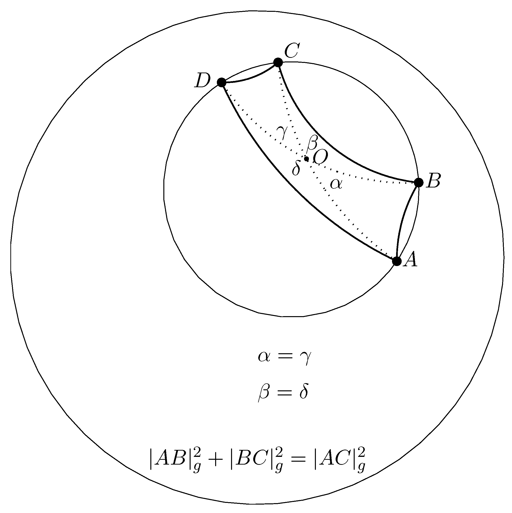
A gyrocyclic gyroquadrilateral is gyrodiametric if its gyrodiagonals intersect at its circumgyrocenter, as shown in Figure 4.
A gyrodiametric gyroquadrilateral , shown in Figure 4, gives rise to the two gyrodiametric gyrotriangles and . In the notation shown in Figure 4 we clearly have
Hence, it follows from (21) that
where , and are the g-modified gyrolengths of the gyrosides of the gyrodiametric gyrotriangle , as shown in Figure 4.
Formalizing the result in (24), we have proved the following theorem, where we use the notation in Figure 4.
Theorem 3.
(Gyrodiametric Gyrotriangle Pythagorean-like Equation).Let be a gyrodiametric gyrotriangle in a Möbius gyrovector space , where is the gyrodiametric gyroside. Then, the gyrotriangle gyrosides obey the Pythagorean-like equation
where
References
- Ungar, A.A. Thomas rotation and the parametrization of the Lorentz transformation group. Found. Phys. Lett. 1988, 1, 57–89. [Google Scholar] [CrossRef]
- Ungar, A.A. A gyrovector space approach to hyperbolic geometry; Morgan & Claypool Pub.: San Rafael, California, 2009. [Google Scholar] [CrossRef]
- Ungar, A.A. Analytic hyperbolic geometry: Mathematical foundations and applications; World Scientific Publishing Co. Pte. Ltd.: Hackensack, NJ, 2005. [Google Scholar] [CrossRef]
- Ungar, A.A. Analytic hyperbolic geometry and Albert Einstein’s special theory of relativity; World Scientific Publishing Co. Pte. Ltd.: Hackensack, NJ, 2008. [Google Scholar]
- Ungar, A.A. Analytic hyperbolic geometry and Albert Einstein’s special theory of relativity, 2nd ed.; World Scientific Publishing Co. Pte. Ltd.: Hackensack, NJ, 2022. [Google Scholar] [CrossRef]
- Ungar, A.A. Gyrovector spaces and their differential geometry. Nonlinear Funct. Anal. Appl. 2005, 10, 791–834. [Google Scholar]
- Ungar, A.A. Hyperbolic triangle centers: The special relativistic approach; Springer-Verlag: New York, 2010. [Google Scholar]
- Ungar, A.A. Ptolemy’s theorem in the relativistic model of analytic hyperbolic geometry. Symmetry 2023, 15, 649. [Google Scholar] [CrossRef]
- Ungar, A.A. Hyperbolic trigonometry in the Einstein relativistic velocity model of hyperbolic geometry. Comput. Math. Appl. 2000, 40, 313–332. [Google Scholar] [CrossRef]
- Ungar, A.A. From Möbius to gyrogroups. Amer. Math. Monthly 2008, 115, 138–144. [Google Scholar] [CrossRef]
Figure 1.
In the gyroformalism of analytic hyperbolic geometry, expressions that describe hyperbolic geometric objects take graceful forms analogous to their Euclidean counterparts. This is illustrated here, where the unique gyroline in a Möbius gyrovector plane through two given points is shown. When the gyroline parameter runs from to ∞ the point runs over the gyroline . In particular, at “time” the point is at , and, owing to the left cancellation law of Möbius addition, at “time” the point is at . The Möbius gyroline equation is shown in the box. The analogies it shares with the Euclidean straight line equation in the vector space approach to Euclidean geometry are obvious.
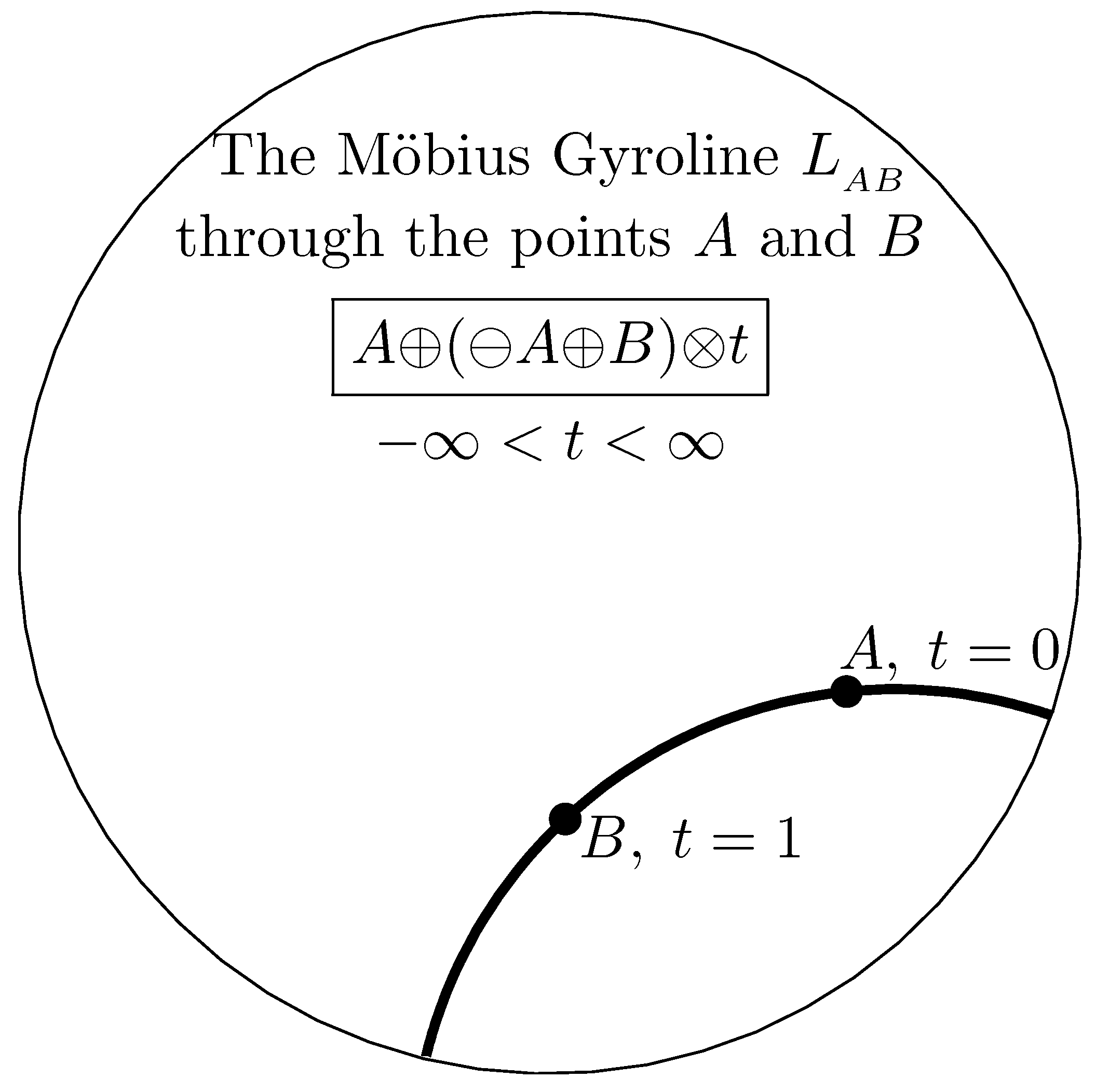
Figure 2.
A gyrotriangle in Möbius gyrovector plane , along with its (i) gyrovertices , (ii) gyroside gyrolengths , and (iii) gyroangles , , and their gyrocosines.
Figure 2.
A gyrotriangle in Möbius gyrovector plane , along with its (i) gyrovertices , (ii) gyroside gyrolengths , and (iii) gyroangles , , and their gyrocosines.
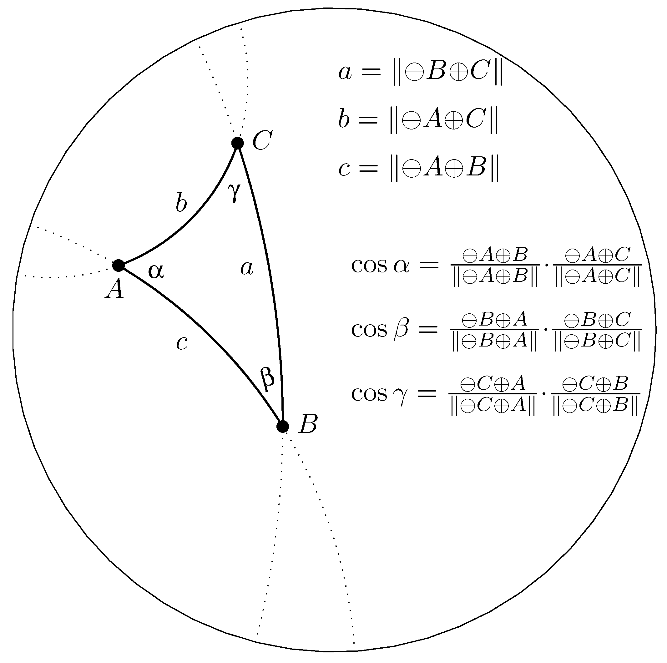
Figure 3.
Illustrating Ptolemy’s Theorem in the hyperbolic plane regulated by Möbius gyrovector plane . A gyrocyclic gyroquadrilateral inscribed in its circumgyrocircle gyrocentered at its circumgyrocenter O, with gyroradius is shown. The O-gyrovertex gyroangles , , and satisfy the equation . The Hyperbolic Ptolemy’s Theorem is fully analogous to its Euclidean counterpart, asserting that , where , , is defined by (20) along with (6).
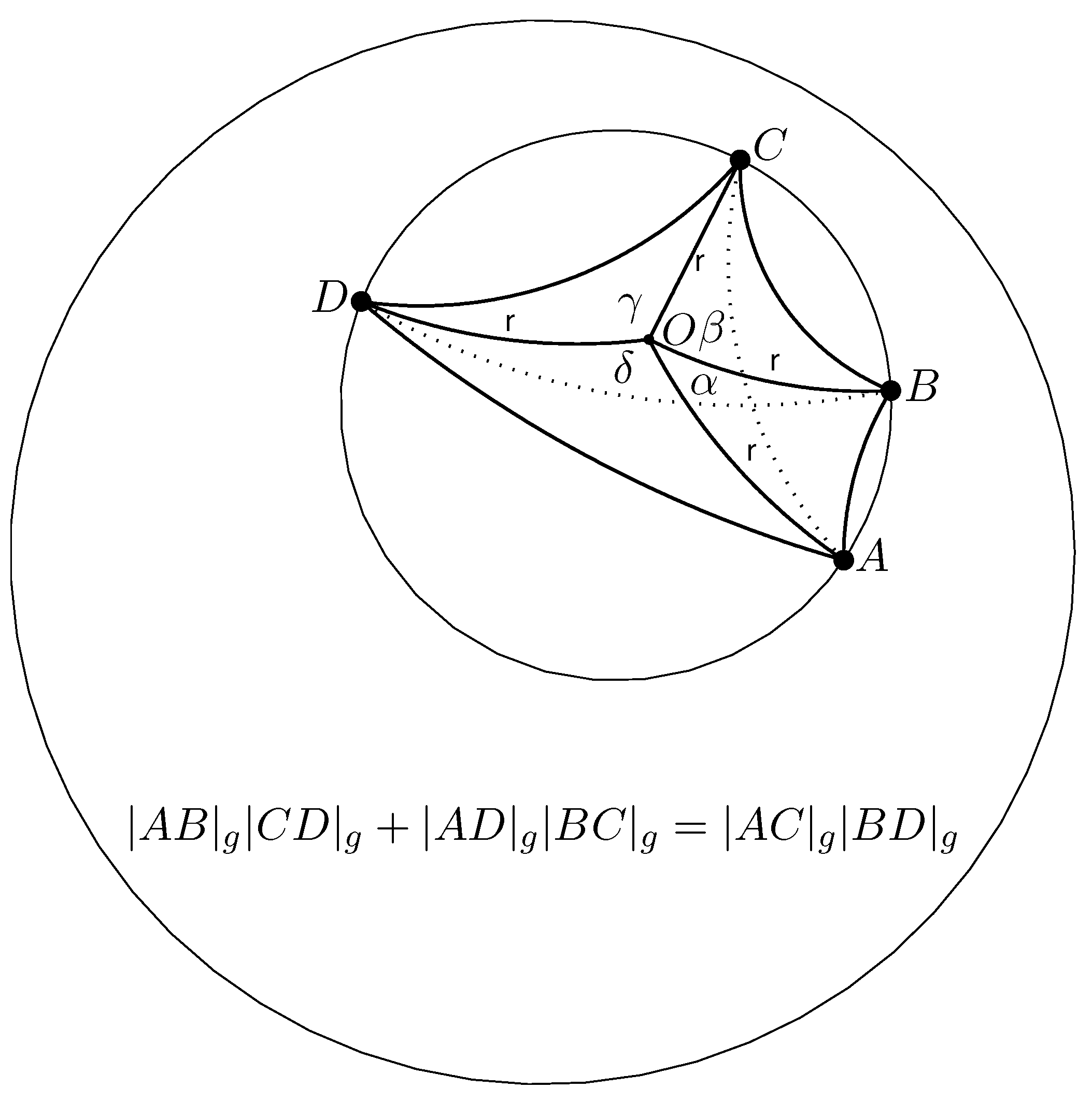
Figure 4.
A Gyrodiametric Gyroquadrilateral in a Möbius gyrovector plane. The gyrocyclic gyroquadrilateral of Figure 3 is depicted here in the special position where the two gyrodiagonals and intersect at the gyroquadrilateral circumgyrocenter O, resulting in the two gyrodiametric gyrotriangles and . The common gyroside, , of these gyrotriangles is a gyrodiameter of the gyroquadrilateral circumgyrocircle. The Pythagorean-like formula that the g-modified gyroside gyrolengths of a gyrodiametric gyrotriangle obey in the Poincaré ball model of hyperbolic geometry is shown.
Disclaimer/Publisher’s Note: The statements, opinions and data contained in all publications are solely those of the individual author(s) and contributor(s) and not of MDPI and/or the editor(s). MDPI and/or the editor(s) disclaim responsibility for any injury to people or property resulting from any ideas, methods, instructions or products referred to in the content. |
© 2023 by the author. Licensee MDPI, Basel, Switzerland. This article is an open access article distributed under the terms and conditions of the Creative Commons Attribution (CC BY) license (http://creativecommons.org/licenses/by/4.0/).
Copyright: This open access article is published under a Creative Commons CC BY 4.0 license, which permit the free download, distribution, and reuse, provided that the author and preprint are cited in any reuse.


