Large Scale Portfolio Optimization Using Biogeography-Based Optimization

Preprint

Article

Large Scale Portfolio Optimization Using Biogeography-Based Optimization

This is a preprint, it has not been peer-reviewed.

Wendy Wijaya^*

,Kuntjoro Adji Sidarto

Wendy Wijaya^*

,Kuntjoro Adji Sidarto

This is a preprint, it has not been peer-reviewed.

Altmetrics

Downloads

118

Views

Comments

Submitted:

21 June 2023

Posted:

22 June 2023

You are already at the latest version

A peer-reviewed article of this preprint also exists.

Abstract

Portfolio optimization is a mathematical formulation whose objective is to maximize returns while minimizing risks. A lot of improvement in the model has been made, including adding practical constraints. With the growing of shares trading, the problem becomes dimensionally very large. In this paper, we propose the usage of modified Biogeography-Based Optimization to solve the large scale constrained portfolio optimization. Results indicate the effectiveness of the method used.

Keywords:

Supplementary Material

supplementary.zip (3.20MB )

1. Introduction

Portfolio can be defined as a collection of assets, which can include cash, real estate, stocks, or crypto. Portfolio optimization concerns about maximizing returns and minimizing risks. Returns are the expected profit from the investment, while risks are the possible changes in values of the investment. [1] proposed using means and variances of the portfolio as the returns and risks measures. Good practice of portfolio optimization is very crucial in investment, since it greatly affects the outcome of the investment. In this paper, we focus on portfolio consisting of correlated stocks.

Model proposed by [1] has been studied by many researchers over the years. Since its introduction, a lot of improvements have been made to the model. Some improvements add discrete and integral constraints. Hence, the resulting model becomes mixed-integer nonlinear programming (MINLP). For instance, [2] and [3] considered adding roundlot constraints, which means that shares must be bought in a multiple of some integers. [2] used FortMP solver, while [3] used DIRECT hybridized with Quasi Newton. With increasing complexity, various techniques also emerged. AUGMECON2 is the state of the art multi-objective MINLP solver. It was introduced by [5] and has been shown to very effective in solving multi-objective MINLP. Recent use of AUGMECON2 in portfolio optimization can be found in [6]. The lack of this method is its computational complexity. [6] noted that for some large dimensional problems, AUGMECON2 did not give a converged solution after 7 days.

To get around the complexity of exact methods, an efficient optimizer is needed. One popular approach is to use metaheuristic algorithms. Metaheuristic algorithms are usually inspired by natural processes in biology, chemistry, physics, or society. Most of the time, it is expected that metaheuristic algorithms can produce near-optimal solutions. And later, exact method will be implemented to get more accuracy, such in [3]. [4] proprosed a series of modified metaheuristic algorithms that exploit the structure of MV model with cardinality and quantity constraints. The metaheuristic algorithms used are genetic algorithm (GA), tabu search (TS), and simulated annealing (SA). To handle the cardinality and quantity constraints, they implemented an algorithm to adjust the solutions.

Another example of metaheuristic algorithm is biogeography-based optimization (BBO). It was developed by [7]. The inspiration comes from the dynamics of the geography of habitats. It basically consists of migration and mutation. Elitism is also added to ensure faster convergence. BBO has been used to solve numerous optimization problems in real world. Some of the newer applications can be found in [9] and [8]. Those studies concluded that BBO is a very powerful optimizer. For MINLP, [10] has shown the effeciency of BBO to solve reliability problems and the results demonstrated the superiority of BBO compared to other metaheuristics. In his approach, the integral and discrete constraints are treated as if they were continuous, but in the function evaluation they are rounded accordingly. This is sensical, since BBO is known for its effectiveness in continuous optimization. One of the reasons why we choose BBO is that its. It requires minimal parameters and is easy to implement.

For application in portfolio optimization, there are some literatures using BBO as the main optimizer. [11] used BBO to solve a portfolio optimization with second-order stochastic dominance constraints. [12] used a variant of BBO called laplacian biogeogeography-based optimization (LX-BBO) to find porfolio allocation from 10 assets in MV model. [13] used BBO to solve constrained MV model and applied the results in forecasting via Monte Carlo. The number of asset used in that research was 15.

Over the time, the number of companies listed in the stock markets are increasing. There are a lot of markets with a really high number of companies. While this provides a good chance for investor to choose assets, this also provides a problem of choosing the suitable assets. [19] studied on how to efficiently choose a subset of large set to optimise a portfolio. He considered a constrained portfolio optimization with cardinality constraint and quantity constraint. His method was inspired by quadratic programming techniques and later improved to worked very well in solving portfolio optimization. [20] considered a multiobjective constrainted mean-variance model and used four methods to solve the problem. The methods he used are Normalized Multiobjective Evolutionary Algorithm based on Decomposition (NMOEA/D), Multiobjective Differential Evolution based on Summation Sorting (MODE-SS) and Multiobjective Differential Evolution based on Nondomination Sorting (MODE-NDS), Multiobjective Comprehensive Learning Particle Swarm Optimizer (MO-CLPSO), and Nondominated Sorting Genetic Algorithm II (NSGA-II). The constraint they added to the model was preselection constraint. They concluded that the methods were efficient for large scale portofolio optimization. They also suggested adding practical constraints such as cardinality constraint and quantity constraint for furthe research.

In this paper, we proposed the usage of [4] heuristic ideas but implemented in BBO framework to solve constrained MV model. The reason we used [4] ideas is that it worked really well on large scale portfolio in their research. The dimensions studied by that research was 31, 85, 89, 98, and 225. Their methods can solve a large scale portofolio optimization problem with high accuracy and in short time. It is clear that standard methods do not solve this problem effectively since the computation complexity is very big.

We use data from ORLibrary which is available online. The same data were used in [4] and [14]. We also compare our results with theirs using the same perfomance metric. Results show the competitiveness of BBO compared to other methods.

The organization of this paper is as follows. Section 2 introduces the problem we solve in this paper and how we solve them. The problem is multiobjective constrained portfolio optimization. Then, we make some introduction about biogeography-based optimizaton (BBO) before detailing the method we propose. Section 3 contains the results of our proposed approach and its comparison with other studies. Conclusions and further improvements are also included in that section.

2. Materials and Methods

2.1. Portfolio Optimization

The aim of this subsection is to introduce the problems discussed in the paper. First, we describe the unconstrained MV model. Then, we discuss the constrained MV model. We follow the formulation used in [14].

2.1.1. Unconstrained MV Model

Suppose there are n assets,

A_{1}, A_{2}, \dots, A_{n}

. Let

x_{1}, x_{2}, \dots, x_{n}

denote the budget share or allocation for the assets. The unconstrained MV model can be written as

\begin{matrix} min \sum_{i = 1}^{n} \sum_{j = 1}^{n} σ_{i, j} x_{i} x_{j}, \end{matrix}

(1)

\begin{matrix} s . t . \sum_{i = 1}^{n} μ_{i} x_{i} \geq R, \end{matrix}

(2)

\begin{matrix} \sum_{i = 1}^{n} x_{i} = 1, \end{matrix}

(3)

\begin{matrix} 0 \leq x_{i} \leq 1, i = 1, 2, \dots, n, \end{matrix}

(4)

where R is the target return,

μ_{i}

is the expected return of the ith asset, and

σ_{i, j} = ρ_{i, j} σ_{i} σ_{j}

is the covariance between the ith and jth asset. Expression (1) indicates the objective is to minimize risk, where variance is taken as the risk measure. Constraint (2) tells that minimum required return is R. Constraint (3) is called the budget constraint, meaning all the budget must be spent in investment. Constraint (4) means the budget share is never negative, so that short selling is not allowed. (1) - (4) altogher is called the unconstrained MV model.

2.1.2. Constrained MV Model

Formally, the constrained MV model is

\begin{matrix} min γ \sum_{i = 1}^{n} \sum_{j = 1}^{n} σ_{i, j} x_{i} x_{j} - (1 - γ) \sum_{i = 1}^{n} μ_{i} x_{i} \end{matrix}

(5)

\begin{matrix} s . t . \sum_{i = 1}^{n} x_{i} = 1, \end{matrix}

(6)

\begin{matrix} \sum_{i = 1}^{n} z_{i} = K, \end{matrix}

(7)

\begin{matrix} ε_{i} z_{i} \leq x_{i} \leq δ_{i} z_{i}, i = 1, 2, \dots, n, \end{matrix}

(8)

\begin{matrix} 0 \leq x_{i} \leq 1, i = 1, 2, \dots, n, \end{matrix}

(9)

where

z_{i} \in {0, 1}

z_{i} = 1

iff the ith asset is in the portfolio. The variable

γ

in expression (5) is the risk attitude parameters. The closer

γ

to 1, the more risk aversity occurs. On the other hand, the closer

γ

to 0, the more risk seeking occurs. So, instead of finding the optimal values to just one value of target return, we will find a set of pareto optimal solutions. Constraint (6) is still the same budget constraint. Constraint (7) is called the cardinality constraint,i.e. the number of assets in the portfolio must be K. Constraint (8) is called the quantity constraint. It is a conditional bound that limits the maximum and minimum of allocation in the individual asset if the asset is in the portfolio.

2.2. Biogeography-Based Optimization

BBO was first introduced by [7]. BBO was inspired by Biogegraphy. Biogeography is the study of relation between geographical factors and organisms. Biogeography mathematically follows the natural process of how species migrate from one habitat to another habitat, how new species emerge, and how species become extinct. Migration consists of two kinds: immigration is when new species enter a new habitat and emigration is when species leave a habitat (but not necessarily fully disappear from the original habitat). Each habitat (mathematically expressed as n-dimensional vectors) has its own characteristics. Each characteristic is called suitability index variable (SIV). Basically, SIV are the decision variables in the optimization problem. Habitat suitability index (HSI) is the fitness value of a habitat. It is the objective function value in the optimization problem. Each habitat is ranked based on the HSI, where in minimization problem, the habitat with higer HSI is ranked better than habitat with lower HSI.

Let

S_{1}, S_{2}, \dots, S_{N}

denote N habitats. Habitat

S_{i}

has exactly i species. The dth SIV of habitat

S_{i}

will be denoted by

S_{i} (d)

. Each habitat have its own immigration rate (

λ_{i}

) and emigration rate (

μ_{i}

). usually, linear immigration and emigration are used. [21]listed some of popular migration rate models, such as constant, linear, trapezoidal, quadratic, and sinusoidal. Each migration model has their own characteristics. In addition to that, they also studied the convergence properties of BBO and some ways on how to improve the convergence based on migration models. If E and I denote the maximum and minimum emigration rate and immigration rate, then

\begin{matrix} λ_{i} = I (1 - \frac{i}{n}) and μ_{i} = E (\frac{i}{n}), i = 0, 1, \dots, N . \end{matrix}

(10)

This is depicted in Figure 1. The higher the number of species means a habitat is already saturated. It will force its species to search for better habitat and prevent more species to enter. Hence, habitat with big number of species will have big emigration rate and small immigration rate.

In BBO, habitat with better HSI will have more species, because it is more suitable to live at. So, a good habitat will affect worse habitat to become better. The migration process in BBO is given by

Algorithm 1 Migration

Input

n, the dimension of the decision variables

$S_{k}$ , current solution

$μ$ , emigration rate

$λ$ , immigration rate
Process

Step 1. Set $i = 1$

Step 2. If $r a n d (0, 1) > λ_{k}$ , go to step 5.

Step 3. Choose a random habitat $S_{l} \sim μ_{l}$ .

Step 4. Replace the ith coordinate of $S_{k}$ with the ith coordinate of $S_{l}$ , $S_{k} (i) = S_{l} (i) .$

Step 5. Set $i = i + 1$ .

Step 6. If $i > n$ stop. Otherwise, go to step 3.
Output

Migrated solution $S_{k}$ .

Another variation of migration process was introduced by [15]. It has a blending parameter

α

which makes migration more random.

α

can be a constant or randomly chosen at each iteration. In this paper, we use constant

α

Algorithm 1b Blended Migration

Input

n, the dimension of the decision variables

$S_{k}$ , current solution

$μ$ , emigration rate

$λ$ , immigration rate

$α \in [0, 1]$ , blending parameter.
Process

Step 1. Set $i = 1$

Step 2. If $r a n d (0, 1) > λ_{k}$ , go to step 5.

Step 3. Choose a random habitat $S_{l} \sim μ_{l}$ .

Step 4. Perform a blending of immigrating and emigrating habitat using $S_{k} (i) = α S_{k} (i) + (1 - α) S_{l} (i) .$

Step 5. Set $i = i + 1$ .

Step 6. If $i > n$ stop. Otherwise, go to step 3.
Output

Migrated solution $S_{k}$ .

Natural events like disaster or pandemic can also happen in a habitat. It will make some unpredictable changes in the habitat. In BBO, this is called mutation. Mutation is more likely to occur in a habitat with high number or low number of species. But, it will be improbable in a habitat with medium number of species. The mutation probability of a habitat is

\begin{matrix} m_{i} = m_{m a x} (1 - \frac{P_{i}}{P_{m a x}}) . \end{matrix}

(11)

P_{i}

denote the probability that a habitat will have species count i and

P_{m a x} = m a x {P_{i} | i = 1, 2, \dots, N}

. According to [18],

P_{i}

is given by

\begin{matrix} P_{i} = \{\begin{matrix} \frac{1}{1 + \sum_{k = 1}^{N} \frac{\prod_{l = 1}^{k} λ_{l - 1}}{\prod_{l = 1}^{k} μ_{l}}}, & i = 0 \\ \frac{\prod_{l = 1}^{i} λ_{l - 1}}{\prod_{l = 1}^{i} μ_{l}} P_{0}, & i = 1, 2, \dots, N \end{matrix} \end{matrix}

(12)

Mutation in BBO is performed based on the following algorithm.

Algorithm 2 Mutation

Input

n, the dimension of the decision variables

$S_{k}$ , current solution

m, mutation probability
Process

Step 1. Set $i = 1$

Step 2. If $r a n d (0, 1) > m_{k}$ , go to step 4.

Step 3. Replace the ith coordinate of $S_{k}$ with a random number inside permissible bounds, $S_{k} (i) = r a n d (l o w e r b o u n d, u p p e r b o u n d)$ .

Step 4. Set $i = i + 1$ .

Step 5. If $i > n$ stop. Otherwise, go to step 3.
Output

Mutated solution $S_{k}$ .

Another component in BBO is the existence of elitism. In short, elitism is the preservation of good habitass. During elitism process, some good habitas from previous generation will replace the worst habitats in next generation. This has a purpose to ensure next generation solution is not worse than the previous generation solution. In their study, [20] proved an interesting results about the convergence of BBO for binary problem. The existence of migration and mutation operators only do not guarantee convergence of the algorithm. But, migration and mutation operators combined with elitism will almost surely produce a convergent solution. Hence, elitism is an essential part of BBO algoritm. In general, BBO can be described as follows.

Algorithm 3 Biogeography-Based Optimization

Input

$M a x G e n$ , maximum number of generations

N, number of habitat

n, dimension of the decision variables

E, maximum emigration rate

I, maximum immigration rate

$m_{m a x}$ , maximum mutation rate

$k e e p$ , number of preserved habitats

$α$ , blending parameter if Blended BBO is used
Process

Step 1. Initialise randomly N habitats in $R^{n}$ .

Step 2. Evaluate the HSI of each habitat and sort the habitats according HSI.

Step 3. Calculate $λ, μ,$ and m.

Step 4. Set $i t e r = 1$ .

Step 5. For $i = 1, 2, \dots, N$ , perform migration according to algorithm 1 or 1b.

Also, perform mutation according to algorithm 2.

Step 6. Sort the new habitats based on HSI.

Step 7. Replace the last $k e e p$ habitats with the first $k e e p$ habitats from previous generation and resort the new population.

Step 8. $i t e r = i t e r + 1$ . If $i t e r > m a x g e n$ , stop. Otherwise, go to step 5.
Output

Return $S_{b e s t}$ (habitat with best HSI) as the best solution.

2.3. Modified BBO

One technique to solve a constrained optimization problem is using penalty function. But, too many penalty functions will have a negative effect in the computational complexity. It also reduces the ability to explore and exploit feasible solutions. Most of candidate solutions are not feasible solutions. A large number of iterations are needed to achieve a convergent solution. For portfolio optimization, [4] developed an efficient scaling algorithm to take care of cardinality constraint and quantity constraint at once. Then, the algorithm is embedded inside three algorithms: GA, TS, and SA. Two interesting results from their research is that the solutions produced are both accurate and need little time.

We propose using the scaling algorithm inside BBO. Also, we use some heuristic ideas from [4]. One of the methods they used is genetic algorithm (GA) heuristics. Since GA is similar to BBO in some ways, we modify BBO algorithm following the idea from GA heuristics. In each iteration, rather than checking all habitats one by one, we only do migration from the good habitats. The best habitat is always chosen. Another habitat is chosen randomly only from small subset of good habitats. Furthermore, migration and mutation occurs iff the ith asset exists in both solutions. This greatly simplifies calculation in the BBO algorithm to focus on a subset of assets exist in good portfolio. The scaling algorithm and modified BBO is given below. This strategy is better than handling the integral constraints using penalty in the objective function, because it will require a lot of resources to find good answer. For example, [16] used a population of 50000 in solving a constrained portfolio optimization consisting of only 5 assets.

Algorithm 4 Scaling

Input

S, current solution which contains Q, the set of K different assets, and $s_{i}$ , the value for the ith asset.

$ε$ , the conditional lower bounds.

$δ$ , the conditional upper bounds.
Process

Step 1. Set $L = \sum_{i \in Q} s_{i}$ and $F = 1 - \sum_{i \in Q} ε_{i}$ .

Step 2. For $i \in Q$ , $w_{i} = ε_{i} + s_{i} \frac{F}{L}$ . $w_{i} = 0 i f i \notin Q$ .

Step 3. $R = {j | w_{j} > δ_{j}}$ .

Step 4. If R is not empty: set $L = \sum_{i \in Q - R} s_{i}$ and $F = 1 - (\sum_{i \in Q - R} ε_{i} + \sum_{i \in R} δ_{i})$ . For $i \in Q - R$ , $w_{i} = ε_{i} + s_{i} \frac{F}{L}$ . $w_{i} = δ_{i}$ if $i \in R$ .

Step 5. Evaluate the objective function at w.

Step 6. Set $s_{i} = w_{i} - ε_{i} .$ for $i \in Q$ .
Output

Returns S, objective function value, and w.

Algorithm 5 Modified BBO for Large Scale Portfolio Optimization

Input

$M a x G e n$ , maximum number of generations

N, number of habitats

n, dimension of the decision variables

E, maximum emigration rate

I, maximum immigration rate

$m_{m a x}$ , maximum mutation rate

$B e s t H a b i t a t$ , limit of the best habitats

$α$ , blending parameter

K, number of assets in the portfolio
Process

Step 1. Initialise randomly N habitats in ${[0, 1]}^{n}$ .

Step 2. Evaluate and update each habitat using algorithm 4. Sort the habitats according HSI.

Step 3. Calculate $λ, μ,$ and m.

Step 4. Set $i t e r = 1$ .

Step 5. Choose a random habitat $S_{j} \sim λ_{j}$ from $B e s t H a b i t a t s$ .

Step 6. Create a new habitat $S *$ according to blended migration of $S_{b e s t}$ and $S_{j}$ .

Step 7. Perform mutation on $S *$ according to algorithm 2.

Step 8. If any coordinate of $S *$ is negative, replace it with 0.

Step 9. Set the assets of $S *$ to be the location of positive coordinates. If the number of assets in $S *$ is less than K, then randomly add assets from $S_{1}$ or $S_{j}$ . If the number of assets in $S *$ is bigger than K, randomly choose some assets, remove it.

Step 10. Evaluate and update $S *$ based on algorithm 4.

Step 11. Replace $S_{w o r s t}$ (habitat with worst HSI) with $S *$ and sort the habitats based on HSI.

Step 12. Set $i t e r = i t e r + 1$ . If $i t e r > M a x G e n$ , stop. Otherwise, go to step 5.
Output

Return $S_{b e s t}$ as the best solution.

3. Results and Conclusions

In this section, we first apply the above ideas to measure its effectiveness. We consider using percentage deviation error as the measure of the model effectiveness as used in [4] and [14]. Let

(v_{i}, r_{i})

denote the pair of variance and return at a point in constrained efficient frontier (CEF) found using proposed method. Let also

(v_{j}^{*}, r_{j}^{*})

denote the point in unconstrained efficient frontier calculated by [4]. For each i, we can find

v_{l}^{*} = m a x {v_{j}^{*} | v_{j}^{*} \leq v_{i}}

and

v_{u}^{*} = m i n {v_{j}^{*} | v_{j}^{*} \geq v_{i}}

. Then,

r = r_{l}^{*} + \frac{v_{i} - v_{l}^{*}}{v_{u}^{*} - v_{l}^{*}} (r_{u}^{*} - r_{l}^{*})

is the approximated return from UEF at

r_{i}

. The vertical deviation error is calculated using

| \frac{r_{i} - r}{r} \times 100 |

. The horizontal deviation error is calculated in a similar fashion. The percentage deviation error is taken as the minimum of the horizontal and vertical deviation error.

3.1. Results

In this section we solve problem (5)-(9) for 50 values of

γ

. We assume

K = 10

(10 assets are chosen for each case),

ε_{i} = 0.01

(the minimum budget allocation for each chosen asset is 0.01), and

δ_{i} = 1

(maximum budget allocation is 1 for each asset). We use the same dataset as [4] and [14]. In total, there are 5 test instances studied. For each instance, we generated 50 points, one point for each value of

γ

γ

will vary from 0 to 1 uniformly. The parameters we use are summarize in Table 1. The comparisons between the proposed method with previous studies are given in Table 2.

3.2. Conclusions

This paper discusses the extensions of the classical MV portfolio model to fit proper real-world situations. The extensions include adding cardinality and quantity constraints which are practical for most investors. The lack of decent approaches to solve the problem, especially the large scale ones, stimulates many alternative approaches. We propose the usage of modified BBO to solve the problem. It uses some ideas from [4] that handle both constraints effectively. The algorithm makes the candidate solutions always satisfy both constraint. This causes the algorithm to yield a convergent result more quickly than letting them evolve wildly.

Table 2, Table 3, Table 4, Table 5 and Table 6 list the points generated by our proposed approach and their average percentage deviation. Figure 2, Figure 3, Figure 4, Figure 5 and Figure 6 shows the unconstrained efficient frontier (UEF) and constrained efficient frontier (CEF) obtained by proposed method. We see that CEF only deviates by a small amount from UEF. From Table 2, we see that modified BBO works pretty well in large scale portfolio optimization. Although GA works best in most instances, modified BBO can still give good near-optimal solutions. Especially, in the third and fourth instances, modified BBO produce lower mean in percentage deviation error than the other methods. The performance of our proposed apporach for the last instance is the worst compared to other methods. To overcome this, more iterations can be performed to the method at the cost of computation time.

Possible improvements can be made to the proposed method, such as using ideas of set-based metaheuristic algorithms to take care of cardinality and quantity constraints separately. Such approach has been studied by some researches, for instance see [17]. The idea is to choose a certain subset of assets first, then optimize the portfolio allocation for each subsets. Looking at various migration and mutation models are also interesting direction to do.

Another possible future research is to consider some more practical constraints such as roundlot constraint, transaction cost, and preselection constraint. The idea of putting in more constraints is so that investor can fully realizes his investment plan. Overall, the performance of the proposed method is satisfying in solving large scale constrained portfolio optimization.

Table 7. Points generated by proposed approach (Nikkei).

Variance	Mean	Average Percentage Deviation
0.001436	0.003803	3.486284
0.001478	0.003866	2.058811
0.001468	0.003840	2.675959
0.001286	0.003836	1.990562
0.001397	0.003838	2.435501
0.001422	0.003873	1.658157
0.001306	0.003828	2.292592
0.001173	0.003823	1.647790
0.001446	0.003823	3.022733
0.001038	0.003744	2.339931
0.000983	0.003757	1.311337
0.001038	0.003776	1.525063
0.001139	0.003778	2.551383
0.001159	0.003837	1.172552
0.001070	0.003797	1.342218
0.000980	0.003762	1.148405
0.000990	0.003773	0.992732
0.000902	0.003717	1.186169
0.000865	0.003686	1.409206
0.000810	0.003647	1.437170
0.000775	0.003580	2.534151
0.000880	0.003648	2.703923
0.000735	0.003579	1.607936
0.000716	0.003566	1.444799
0.000756	0.003585	1.977517
0.000691	0.003543	1.303900
0.000705	0.003531	2.075318
0.000752	0.003591	1.704716
0.000738	0.003571	1.894145
0.000714	0.003549	1.854665
0.000673	0.003471	2.630567
0.000621	0.003410	1.686711
0.000638	0.003435	2.032659
0.000659	0.003371	4.875107
0.000591	0.003323	1.767862
0.000652	0.003437	2.680428
0.000603	0.003326	2.806483
0.000597	0.003317	2.583661
0.000611	0.003356	2.590976
0.000581	0.003260	2.513779
0.000570	0.003229	1.894738
0.000585	0.003237	3.695110
0.000571	0.003217	2.406920
0.000519	0.002910	3.618237
0.000455	0.002414	5.148647
0.000399	0.001842	6.038083
0.000360	0.001213	7.445995
0.000349	0.001010	6.993303
0.000330	0.000448	7.172271
0.000321	-0.000113	5.414716

Author Contributions

Supervision, K.A.S.; Writing—original draft, W.W.

Funding

This research was funded by LPDP.

Data Availability Statement

The data used in this paper are available at https://github.com/CYLOL2019/Portfolio-Instances/tree/master/OR-Library.

Acknowledgments

The authors are grateful to LPDP for facilitating the funding of this paper.

Conflicts of Interest

The authors declare no conflict of interest.

References

Markowitz, H. Portfolio Selection. J. Finance 1952, 7, 77–91.
Jobst, Norbert J., Michael D. Horniman, Cormac A. Lucas, and Gautam Mitra. Computational aspects of alternative portfolio selection models in the presence of discrete asset choice constraints. Quant. Finance 2001, 1, 489–501. [CrossRef]
Bartholomew-Biggs, Mike C., and Stephen. J. Kane. A global optimization problem in portfolio selection. Comput. Manag. Sci. 2009, 6, 329–345. [CrossRef]
T. J. Chang, N. Meade, J.E. Beasley, and Y.M. Sharaiha. Heuristics for cardinality constrained portfolio optimisation .Comput. Oper. Res. 2000, 27, 1271–1302. [CrossRef]
Mavrotas, G. and Florios, K. An improved version of the augmented ϵ-constraint method (AUGMECON2) for finding the exact pareto set in multi-objective integer programming problems. Appl. Math. Comput. 2013, 219(18), 9652–9669. [CrossRef]
Chen, Y., Zhou, A. and Das, S. Utilizing dependence among variables in evolutionary algorithms for mixed-integer programming: A case study on multi-objective constrained portfolio optimization. Swarm Evol. Comput. 2021, 66, 100928. [CrossRef]
Simon, D. Biogeography-based optimization. IEEE Trans. Evol. 2008, 12(6), 702–713.
Ren, H., Guo, C., Yang, R., and Wang, S. Fault diagnosis of electric rudder based on self-organizing differential hybrid biogeography algorithm optimized neural network. Meas. 2023, 208, 112355. [CrossRef]
Reihanian, A., Feizi-Derakhshi, M.R., and Aghdasi, H.S. An enhanced multi-objective biogeography-based optimization for overlapping community detection in social networks with node attributes. Inf. Sci. 2023, 622, 903–929. [CrossRef]
Garg, H. An efficient biogeography based optimization algorithm for solving reliability optimization problems. Swarm Evol. Comput. 2015, 24, 1–10. [CrossRef]
Ye, T., Yang, Z., and Feng, S. Biogeography-based optimization of the portfolio optimization problem with second order stochastic dominance constraints. Algorithms 2017, 10(3), 100. [CrossRef]
Garg, V. and Deep, K. Portfolio optimization using Laplacian biogeography based optimization. Opsearch 2019, 56, 1117-1141. [CrossRef]
Panwar, D., Jha, M., and Srivastava, N. Portfolio selection using Biogeography-based optimization & Forecasting. J. Adv. Res. Dyn. Control Syst. 2018, 10(6), 852–863.
Kabbani, T. Metaheuristic Approach to Solve Portfolio Selection Problem. arXiv preprint arXiv:2211.17193. arXiv:2211.17193.
Ma, H. and Simon, D. lended biogeography-based optimization for constrained optimization. Eng. Appl. Artif. Intell. 2011, 24(3), 517–525.
Febrianti, W., Sidarto, K.A. and Sumarti, N. Solving Constrained Mean-Variance Portfolio Optimization Problems Using Spiral Optimization Algorithm. Int. J. Financ. Stud. 2022, 11(1), 1. [CrossRef]
Erwin, K. and Engelbrecht, A. Multi-Guide Set-Based Particle Swarm Optimization for Multi-Objective Portfolio Optimization. Algorithms 2023, 16(2), 62. [CrossRef]
Wei, L., Zhang, Q., and Yang, B. Improved Biogeography-Based Optimization Algorithm Based on Hybrid Migration and Dual-Mode Mutation Strategy. Fractal fract. 2022, 6(10), 597. [CrossRef]
Perold, A. F. Large-scale portfolio optimization. Manage. Sci. 1984, 30(10), 1143-1160. [CrossRef]
Qu, B. Y., Zhou, Q., Xiao, J. M., Liang, J. J., and Suganthan, P. N. Large-scale portfolio optimization using multiobjective evolutionary algorithms and preselection methods. Math. Probl. Eng. 2017. [CrossRef]
Guo, W., Wang, L., Wu, Q. An analysis of the migration rates for biogeography-based optimization.. Inf. Sci. 2014, 254, 111-140. [CrossRef]
Ma, H., Simon, D., Fei, M. On the convergence of biogeography-based optimization for binary problems. Math. Probl. Eng. 2014. [CrossRef]

Figure 1. Immigration rate and Emigration rate ([7]).

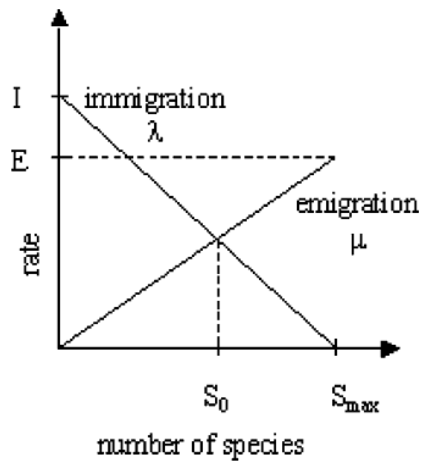
Figure 2. Constrained Efficient Frontier for Hang Seng.

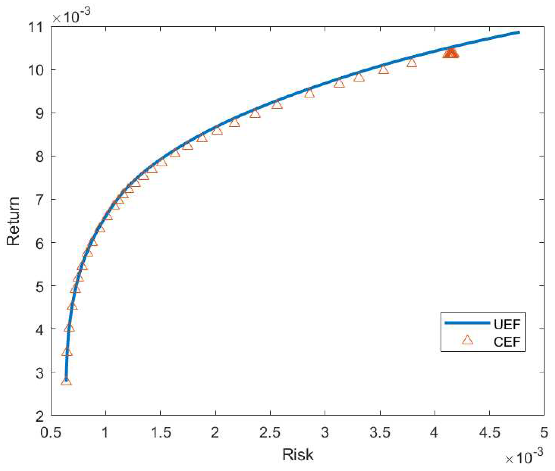
Figure 3. Constrained Efficient Frontier for DAX.

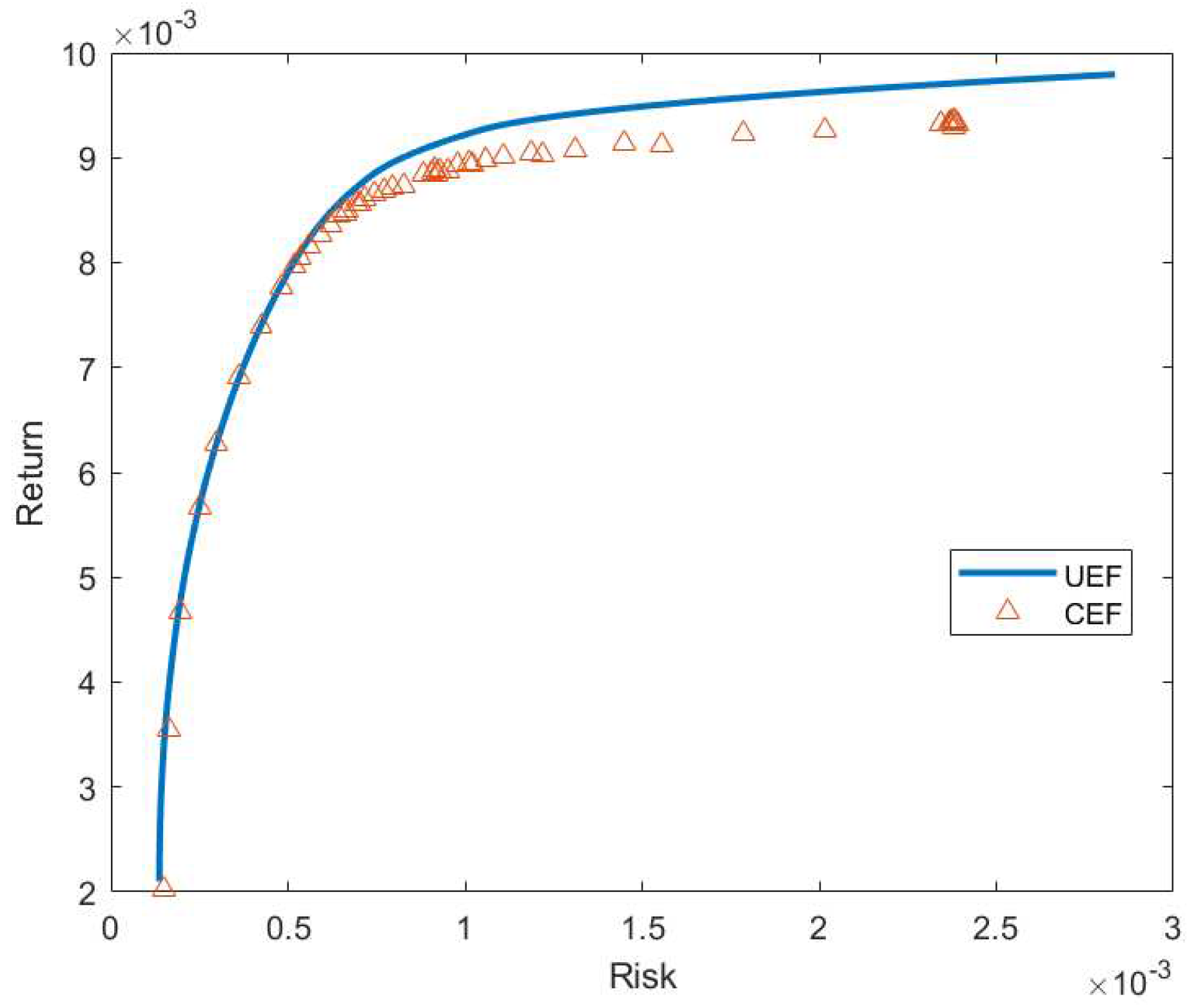
Figure 4. Constrained Efficient Frontier for FTSE.

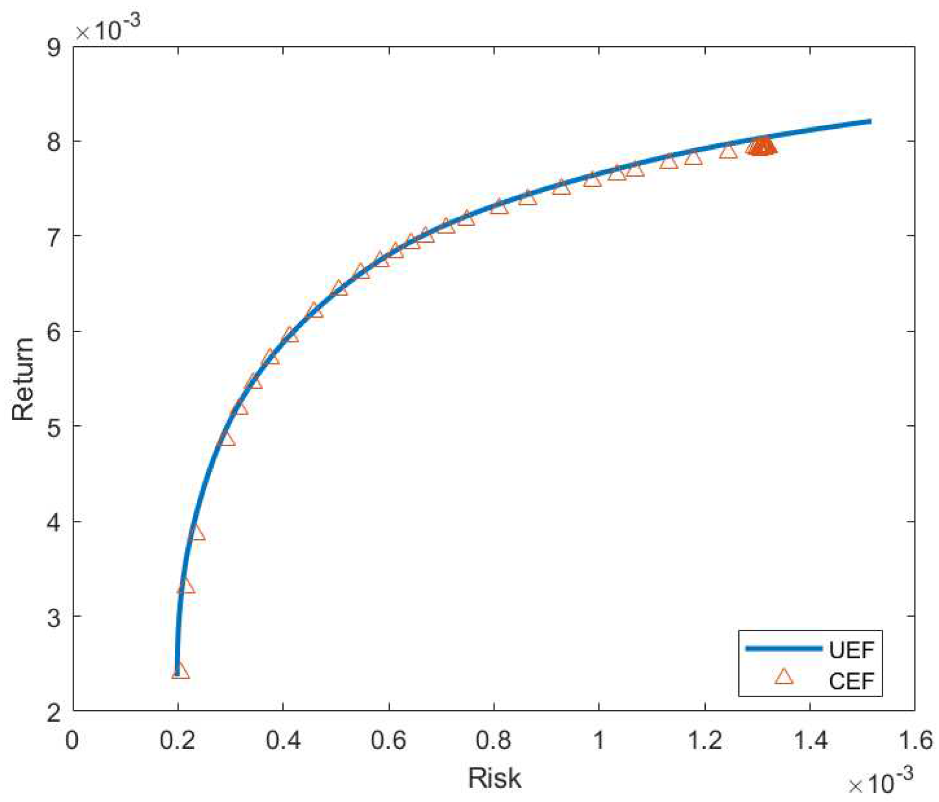
Figure 5. Constrained Efficient Frontier for S&P.

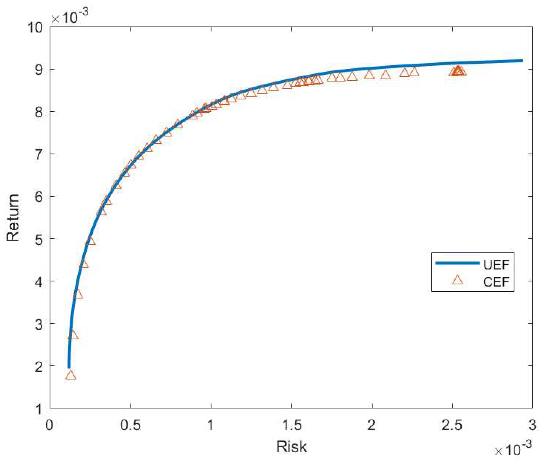
Figure 6. Constrained Efficient Frontier for Nikkei.

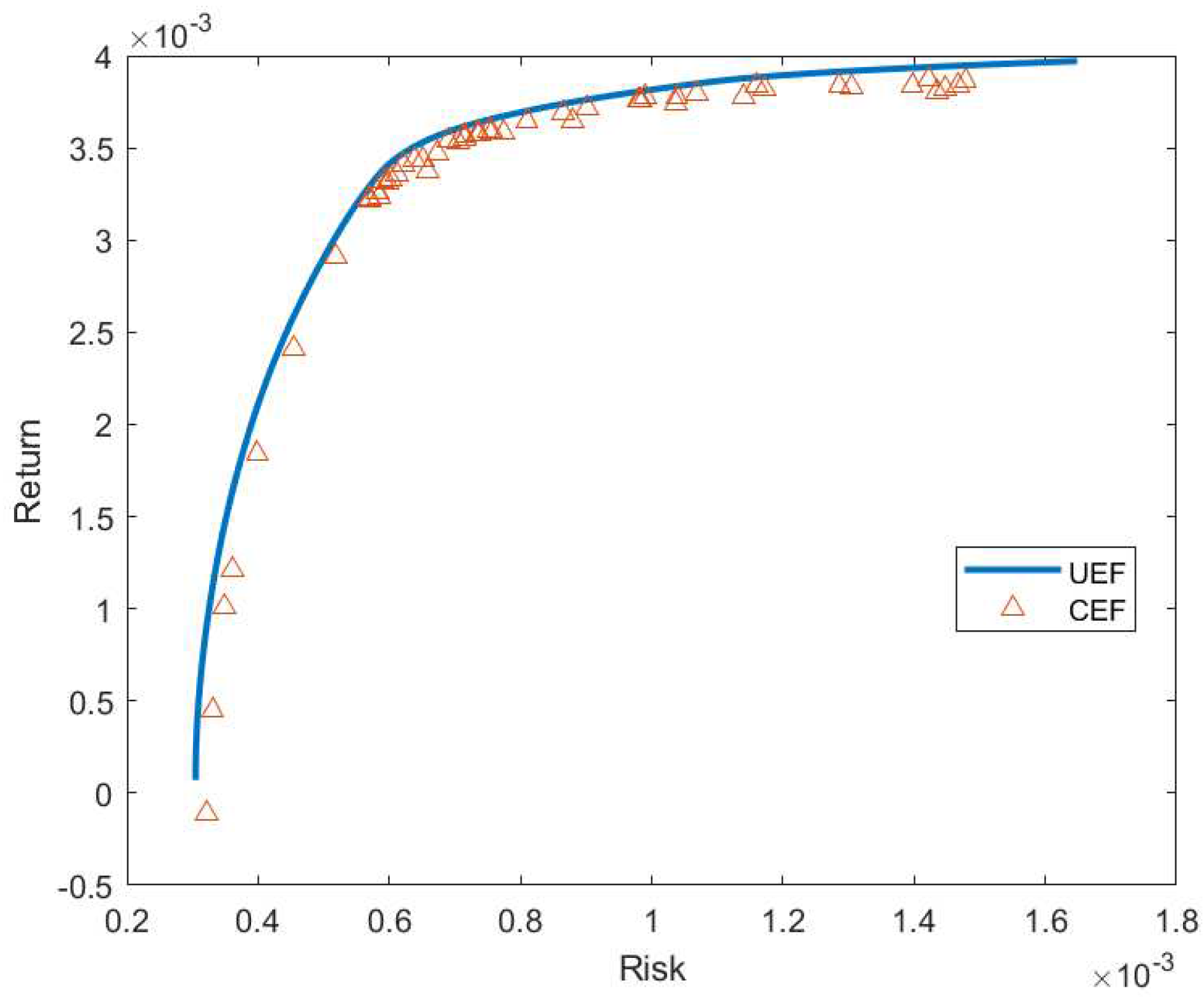
Table 1. Parameters in Modified BBO.

Parameter	Value
n	31, 85, 89 98, and 225
$M a x G e n$	1500n
N	100
E	1
I	1
$m_{m a x}$	0.05
$B e s t H a b i t a t$	10

Table 2. Comparison of performance.

Index	Number of Assets	Percentage Error	GA	TS	SA	TS&TR	BBO
Hang Seng	31	Median	1.2181	1.2181	1.2181	1.8120	1.2503
Hang Seng	31	Mean	1.0974	1.1217	1.0957	2.2656	1.1689
DAX	85	Median	2.5466	2.6380	2.5661	4.2100	2.8845
DAX	85	Mean	2.5424	3.3049	2.9297	4.0350	2.7018
FTSE	89	Median	1.0841	1.0841	1.0841	1.2406	1.1232
FTSE	89	Mean	1.1076	1.6080	1.4623	1.2959	1.1056
S&P	98	Median	1.2244	1.2882	1.1823	2.3630	1.3671
S&P	98	Mean	1.9328	3.3092	3.0696	2.5068	1.8782
NIKKEI	225	Median	0.6133	0.6093	0.6066	1.3464	2.1840
NIKKEI	225	Mean	0.7961	0.8975	0.6732	1.2122	2.6556

Table 3. Points generated by proposed approach (Hang Seng).

Variance	Mean	Average Percentage Deviation
0.004153	0.010344	1.650583
0.004163	0.010352	1.629552
0.004147	0.010349	1.572344
0.004146	0.010340	1.647269
0.004153	0.010348	1.612139
0.004159	0.010358	1.551008
0.004170	0.010347	1.713553
0.004157	0.010342	1.689939
0.004172	0.010356	1.647128
0.004157	0.010357	1.551429
0.004161	0.010355	1.587801
0.004161	0.010358	1.554144
0.004135	0.010336	1.622853
0.004158	0.010357	1.550238
0.004140	0.010351	1.512770
0.004136	0.010342	1.572603
0.004138	0.010342	1.579541
0.004157	0.010357	1.551161
0.004119	0.010338	1.510569
0.003791	0.010138	1.448290
0.003535	0.009970	1.348079
0.003308	0.009805	1.279641
0.003133	0.009666	1.282537
0.002857	0.009436	1.257103
0.002563	0.009165	1.272886
0.002360	0.008962	1.266990
0.002174	0.008750	1.382221
0.002020	0.008570	1.378100
0.001878	0.008400	1.237448
0.001748	0.008218	1.234975
0.001634	0.008044	1.258869
0.001515	0.007841	1.352700
0.001423	0.007682	1.245660
0.001345	0.007526	1.264346
0.001270	0.007368	1.156316
0.001209	0.007222	1.117305
0.001162	0.007098	1.034934
0.001121	0.006972	1.005684
0.001079	0.006841	0.872697
0.001014	0.006598	0.919845
0.000943	0.006313	0.749057
0.000880	0.006004	0.843348
0.000833	0.005748	0.809055
0.000785	0.005442	0.547040
0.000753	0.005183	0.274540
0.000725	0.004910	0.105097
0.000695	0.004509	0.051942
0.000668	0.004020	0.000245
0.000651	0.003462	0.046565
0.000642	0.002783	0.000220

Table 4. Points generated by proposed approach (DAX).

Variance	Mean	Average Percentage Deviation
0.002382	0.009294	4.271820
0.002382	0.009334	3.859833
0.002389	0.009321	4.010914
0.002373	0.009335	3.836193
0.002380	0.009350	3.693022
0.002380	0.009354	3.659281
0.002366	0.009328	3.893850
0.002367	0.009330	3.875557
0.002343	0.009329	3.833951
0.002016	0.009267	3.770710
0.001787	0.009222	3.662769
0.001554	0.009125	4.003385
0.001449	0.009131	3.589703
0.001312	0.009081	3.588020
0.001219	0.009034	3.667880
0.001185	0.009038	3.441760
0.001109	0.009005	3.331500
0.001060	0.008985	3.165848
0.001022	0.008932	3.355975
0.001010	0.008951	3.022658
0.000977	0.008926	2.925377
0.000951	0.008871	3.221054
0.000928	0.008877	2.879177
0.000919	0.008837	3.198529
0.000908	0.008858	2.825535
0.000915	0.008880	2.684058
0.000884	0.008845	2.648340
0.000828	0.008728	3.088740
0.000794	0.008714	2.646350
0.000772	0.008679	2.601097
0.000743	0.008651	2.231962
0.000717	0.008602	2.045399
0.000703	0.008565	2.060150
0.000692	0.008557	1.807666
0.000667	0.008495	1.684501
0.000661	0.008470	1.761572
0.000644	0.008445	1.421802
0.000622	0.008356	1.563716
0.000591	0.008270	1.147955
0.000559	0.008155	0.846998
0.000535	0.008046	0.652199
0.000518	0.007972	0.460661
0.000480	0.007766	0.202550
0.000424	0.007398	0.052871
0.000363	0.006909	0.008647
0.000298	0.006272	0.120913
0.000252	0.005672	0.639808
0.000197	0.004670	2.738101
0.000164	0.003548	7.399037
0.000148	0.002026	8.293337

Table 5. Points generated by proposed approach (FTSE).

Variance	Mean	Average Percentage Deviation
0.001313	0.007922	1.430395
0.001321	0.007936	1.347307
0.001315	0.007943	1.192734
0.001314	0.007944	1.171317
0.001310	0.007936	1.224795
0.001307	0.007932	1.239578
0.001311	0.007933	1.273862
0.001313	0.007936	1.259886
0.001314	0.007939	1.226736
0.001307	0.007936	1.185736
0.001311	0.007929	1.323217
0.001305	0.007897	1.646944
0.001314	0.007929	1.351824
0.001316	0.007940	1.238021
0.001315	0.007923	1.446001
0.001314	0.007934	1.293457
0.001318	0.007926	1.444648
0.001315	0.007937	1.270114
0.001303	0.007925	1.282893
0.001319	0.007936	1.327979
0.001313	0.007936	1.257175
0.001304	0.007925	1.291514
0.001298	0.007923	1.240553
0.001294	0.007926	1.150649
0.001245	0.007875	1.192599
0.001178	0.007811	1.087917
0.001132	0.007768	0.929335
0.001067	0.007689	0.845078
0.001033	0.007645	0.797961
0.000987	0.007578	0.797368
0.000928	0.007492	0.712365
0.000863	0.007390	0.626987
0.000810	0.007291	0.622903
0.000747	0.007170	0.519232
0.000710	0.007088	0.469513
0.000671	0.006994	0.386378
0.000642	0.006922	0.250097
0.000612	0.006834	0.139266
0.000583	0.006735	0.121339
0.000548	0.006606	0.062273
0.000505	0.006426	0.013625
0.000457	0.006200	0.031785
0.000411	0.005945	0.063716
0.000375	0.005710	0.090941
0.000343	0.005446	0.524856
0.000315	0.005175	1.015483
0.000292	0.004851	2.492365
0.000235	0.003865	4.206109
0.000216	0.003307	3.878245
0.000206	0.002404	3.798280

Table 6. Points generated by proposed approach (S&P).

Variance	Mean	Average Percentage Deviation
0.002529	0.008922	2.359602
0.002557	0.008929	2.340721
0.002541	0.008919	2.416129
0.002534	0.008933	2.249225
0.002538	0.008937	2.211467
0.002539	0.008936	2.228023
0.002507	0.008902	2.541732
0.002263	0.008899	2.062808
0.002203	0.008884	2.073489
0.002087	0.008842	2.221486
0.001985	0.008841	1.910974
0.001879	0.008807	1.899560
0.001805	0.008783	1.846467
0.001751	0.008775	1.654681
0.001666	0.008734	1.513308
0.001650	0.008706	1.697012
0.001605	0.008711	1.298059
0.001611	0.008696	1.516222
0.001575	0.008676	1.449458
0.001557	0.008677	1.290429
0.001528	0.008663	1.208081
0.001475	0.008601	1.440881
0.001391	0.008547	1.263060
0.001320	0.008483	1.262410
0.001251	0.008422	1.176603
0.001186	0.008355	1.102604
0.001127	0.008289	0.982920
0.001086	0.008227	1.014893
0.001085	0.008239	0.845325
0.001034	0.008156	0.780838
0.001006	0.008109	0.718416
0.000971	0.008061	0.429940
0.000960	0.008040	0.419244
0.000913	0.007958	0.197980
0.000887	0.007899	0.195589
0.000795	0.007679	0.201780
0.000724	0.007490	0.179496
0.000662	0.007310	0.107246
0.000604	0.007125	0.040827
0.000553	0.006938	0.015456
0.000503	0.006726	0.030648
0.000466	0.006549	0.058691
0.000411	0.006253	0.268371
0.000354	0.005883	0.626792
0.000322	0.005624	1.141503
0.000252	0.004932	2.785801
0.000212	0.004385	4.377882
0.000175	0.003671	8.775220
0.000144	0.002706	12.135965
0.000133	0.001754	9.777885

Disclaimer/Publisher’s Note: The statements, opinions and data contained in all publications are solely those of the individual author(s) and contributor(s) and not of MDPI and/or the editor(s). MDPI and/or the editor(s) disclaim responsibility for any injury to people or property resulting from any ideas, methods, instructions or products referred to in the content.

© 2023 by the authors. Licensee MDPI, Basel, Switzerland. This article is an open access article distributed under the terms and conditions of the Creative Commons Attribution (CC BY) license (http://creativecommons.org/licenses/by/4.0/).

Copyright: This open access article is published under a Creative Commons CC BY 4.0 license, which permit the free download, distribution, and reuse, provided that the author and preprint are cited in any reuse.

Alerts

MDPI Initiatives

Important Links

Choose an area of interest and we will send you notifications of new preprints at your preferred frequency.

Disclaimer

Large Scale Portfolio Optimization Using Biogeography-Based Optimization

Abstract

1. Introduction

2. Materials and Methods

2.1. Portfolio Optimization

2.1.1. Unconstrained MV Model

2.1.2. Constrained MV Model

2.2. Biogeography-Based Optimization

2.3. Modified BBO

3. Results and Conclusions

3.1. Results

3.2. Conclusions

Author Contributions

Funding

Data Availability Statement

Acknowledgments

Conflicts of Interest

References

MDPI Initiatives

Important Links

Subscribe