Submitted:
21 June 2023
Posted:
21 June 2023
You are already at the latest version
Abstract
Accurate seasonal weather forecasts are vital across a broad spectrum of applications, bearing significant environmental and socioeconomic implications. This importance renders the subject a matter of primary interest to a wide range of stakeholders, including the general public, agricultural sector, emergency responders, financial institutions, and policy strategists. The need for precision in long-term predictive models necessitates the development of innovative methodologies. These methodologies should be capable of deciphering atmospheric patterns and mechanisms with detail, especially at a local level, without the resource constraints that dynamical downscaling imposes. In response to this expanding demand, this study presents a novel solution, combining a stochastic deep learning methodology, specifically Generative Adversarial Networks (GANs), with a Digital Elevation Model (DEM). The cornerstone of the proposed model is the enhancement of gridded temperature fields from seasonal forecasts. The area of focus was the Hellenic region, wherein the spatial resolution is amplified from a coarse 1° x 1° grid to an impressively detailed 0.1° x 0.1° grid. This offers a transformative perspective for interpreting and employing this crucial meteorological data. The results suggest that the downscaled fields adequately approximate the actual spatial distribution, although the predicted values tend to slightly overestimate and in some cases underestimate the original ones. This study underlines the potential of this approach to significantly enhance the resolution and utility of weather forecasts, thereby contributing to a variety of sectors dependent on reliable meteorological data.
Keywords:
generative adversarial networks
; downscaling
; seasonal forecasts
; ERA5-Land
; EU-DEM
1. Introduction
Improving sub-seasonal to seasonal forecasts (S2S) is particularly critical and challenging. Accurate seasonal predictions are essential for providing decision-makers with information on potential extreme events risks or opportunities to optimize resource management [1]. The predictability in this time range is frequently low or only slightly better than climatology or persistence forecasts [2]. It is heavily reliant on the existence of active sources of S2S predictability, also known as “windows of opportunity” [3]. Unlike weather forecasts, predictive ability on extended time scales can capitalize on particular climate phenomena or conditions to generate a discernible signal above weather noise. Presently, it is recognized that such conditions occur sporadically over time and have spatially diverse effects on predictability, thereby offering frequent windows of opportunity for skillful forecasts [1].
The accuracy of seasonal forecasts can indeed depend on latitude, as well as other factors such as geographical location, local climate, and the specific climate model used for forecasting. Generally, seasonal forecasts tend to be more accurate in the tropics and less accurate at higher latitudes. Several factors contribute to the difference in forecast accuracy between tropical regions and higher latitudes. Firstly, tropical climates are primarily influenced by large-scale dynamical processes like the El Niño-Southern Oscillation (ENSO) and the Madden-Julian Oscillation (MJO), which can be relatively well-represented in climate models, leading to more accurate seasonal forecasts for these regions. In contrast, higher latitudes are influenced by local factors such as land-sea contrasts, complex topography, and smaller-scale weather systems, which are more challenging to model and predict, resulting in reduced forecast accuracy. Additionally, the signal-to-noise ratio, which compares the strength of the climate signal to weather variability, is typically higher in the tropics, making it easier to detect and predict the underlying climate signal. Lastly, climate models often have coarser resolution at higher latitudes, limiting their ability to capture small-scale processes and features like sea ice, snow cover, and land-sea interactions, and leading to more pronounced model biases, which can affect seasonal forecast accuracy.
Global Climate Models (GCMs) operate at an exceedingly coarse resolution, frequently utilizing grids larger than 100km x 100km. This level of coarseness is unsuitable for numerous applications. Consequently, various downscaling methods have been proposed to address this issue. There are two primary approaches to downscaling climate model outputs: Statistical and Dynamical downscaling.
In the case of Dynamical downscaling, a high-resolution climate model is employed, commonly referred to as a regional climate model (RCM). RCMs utilize lower resolution climate models, such as GCMs in most instances, as boundary conditions, and apply physical principles to simulate local climate conditions. Due to their computational intensity, RCM output data may be limited for certain regions.
If RCM data is either unavailable for a specific region or deemed excessively coarse, Statistical downscaling can be employed as an alternative. Numerous statistical downscaling methodologies have been established to cater to a variety of situations. A crucial aspect of statistical downscaling is the accessibility of local weather data. The quality and duration of historical observed weather data directly impact the accuracy of statistical downscaling outcomes. If a comprehensive dataset is available for a particular weather station (or multiple stations), the climate model can be downscaled to accommodate that specific station. Likewise, if a well-developed gridded dataset is available, downscaling can be adjusted to fit that grid.
Artificial Intelligence (AI) is revolutionizing computer technology and holds great promise for transforming weather forecasting, climate monitoring, and decadal prediction [3]. Leveraging AI techniques can reduce human effort, optimize computing resources, and enhance forecast quality. Especially with regards to the downscaling of climate information, deep learning techniques from the field of AI showcase a promising solution. Deep Learning (DL) [4], a specific subset of Machine Learning (ML) and Artificial Intelligence (AI), has recently emerged as a robust advancement of neural networks. It has significantly enhanced the state-of-the-art in image, video, and speech processing, and is quickly expanding to other application areas. DL is a completely data-driven method that uncovers relationships between input and output data, often unattainable through explicit analytical or physical analysis, by training on reference input datasets and corresponding labeled output data. While various training algorithms exist, the backpropagation algorithm has remained the most popular for many years [3]. With the continuous growth of “big data” and computing power, particularly through specialized hardware like GPUs, the process of identifying hidden relationships within the data has become more efficient in terms of human effort when compared to traditional approaches that require manually designed feature extractors used in conventional machine learning, classification, and pattern recognition or models that convert available input data into desired output data [3].
Various research has been conducted utilizing deep learning for the purposes of downscaling meteorological variables. For example, Lianfa Li (2019) [5] used a deep residual network and reanalysis weather data at a coarse resolution to obtain more consistent and with a better spatial variation of wind speed observation data. In the work of Höhlein et al. (2020) [6], deep learning architectures are proposed that are able to infer situation-dependent wind structures that cannot be reconstructed by other models. For the surface temperature fields, Deep Convolutional Neural Networks (DCNN) are explored in the work of Sekiyama (2020) [7] converting images of low-resolution dynamic models to high-resolution images, utilizing a 22-km gridded global analysis of surface temperature and winds. They demonstrated that the DCNN is capable of estimating the locations of coastlines and mountain ridges in great detail, which are not retained in the inputs, and providing high-resolution surface temperature distributions.
In the scientific discourse surrounding artificial intelligence (AI), its ability to enhance Subseasonal-to-Seasonal (S2S) forecasts has emerged as a promising area of study. This largely stems from AI’s innate capability to agnostically probe expansive multimodel forecasts and observed datasets, revealing emergent patterns within the data [3]. This diverges from traditional methods which involve the a priori reduction of data into constrained subspaces and variables. Notwithstanding, the limited size of model reforecast data for AI training presents a significant hurdle. Consequently, the World Meteorological Organization (WMO) has pinpointed AI as a critical research avenue in weather and climate science in the forthcoming years. The recent results of the S2S competition organized by the WWRP–WCRP S2S project in collaboration with the Swiss Data Science Center (SDSC) and the European Centre for Medium-Range Weather Forecasts (ECMWF), pin-pointed winning algorithms that enhance the S2S forecasts including random forest classification, convolutional neural networks and multiple linear regression [3].
Generative Adversarial Networks have recently been gaining attention in downscaling meteorological fields. For example, in 2020, Leinonen et al. [8] presented a stochastic super-resolution Generative Adversarial Network (GAN) capable of generating a variety of credible high-resolution outputs from a single input. Their work utilized radar-measured precipitation from Switzerland and cloud optical thickness derived from the Geostationary Earth Observing Satellite. In the work of Singh et al. (2020) [9] GANs are tested to downscale wind speed fields and their finding showed that the bicubic and SR-CNN methods perform better than ESRGAN on coarse metrics such as MSE. However, the high frequency power spectrum is captured remarkably well by the GAN, virtually identical to the real data. In 2022 10. Harris et al. [10] used high-resolution radar measurements to serve as the “ground truth” and the task for the neural network here is to add resolution and structure, while acknowledging non-negligible forecast errors. The study showcases that Generative Adversarial Networks (GANs) and Variational Autoencoder GANs (VAE-GANs) can mirror the statistical characteristics of cutting-edge pointwise post-processing methods, all while producing high-resolution, spatially coherent precipitation maps.
This work, benefitted from the plethora of weather and climate datasets produced by the reSilienT fARminG by Adaptive microclimaTe managEment (STARGATE) project and developed a deep learning approach based on GANs to downscale the crude seasonal forecasts to higher spatial resolutions by utilizing available re-analysis data sets. The seasonal forecasts are targeted -with all the challenges that accompany such tasks- aiming to provide a solid methodology to enhance their spatial resolution. The focus lies in seasonal forecasting of temperature fields at 2m height that in the particular case of Greece is challenging due to its complex topography and coastlines.
In Section 2.1 the GAN methodology is presented; particular focus is placed on the meteorological fields in relation to downscaling in Section 2.2. In Section 2.3 the training data sets and the predictors for the model are presented. In Section 2.4, the Deep-Convolutional GAN architecture is presented, along with the evaluation metrics and the information on the hardware and training timing in GPU. The results are presented in Section 3 and the conclusion of this work is presented in Section 4.
2. Materials and Methods
2.1. Generative Adversarial Networks
The production of atmospheric information using numerical models is intrinsically linked to practical challenges, such as lengthy calculations time-wise, vast output ensembles and difficulties in evaluating the results. Oftentimes, the use of supercomputers can significantly mitigate these challenges, but the required amount of samples rises exponentially with model dimension, highlighting new statistical approaches as more sustainable solutions. In this context, it is essential to leverage recent progress in the field of machine learning and find new applications for generative models, in order to devise a new pathway around some of the most prominent challenges inherent to atmospheric simulations.
Generative models are a collection encompassing a variety of tools and in recent years they have gained the interest of the machine learning community. In principle, they are able to learn a probability distribution from a large set of provided samples and provide a means for rapidly generating new samples that follow that approximated distribution [11]. In other words, a generative model is a tool capable of generating random samples, used for representing some system or process. Generative adversarial networks (GANs) were initially described by Goodfellow et al. (2014) [12] and since then they have evolved into a powerful machine learning technique. GANs are typically composed of two neural networks, the generator and the discriminator, both of which perform a distinct function (Figure 1). The generator accepts a set of random numbers as input and attempts to produce samples (‘fake data’) with the same characteristics as those drawn from a given distribution (‘real data’), whereas the discriminator learns to differentiate between both distributions and assigns a probability that describes its estimate of a sample being drawn from the real data distribution. Both are trained simultaneously in competition with each other, while each network seeks to outperform the other, until a balance is reached. If the process of training is successful, the output of the generator is indistinguishable from the training dataset and samples from the generator can be used as if they originated from the target distribution.
Since the GANs first made their appearance, numerous architectures, loss functions, and training approaches have emerged. Among the most important GAN variations are deep convolutional GANs (DCGANs), as their usage of convolutional layers renders them more suitable for computer vision applications and higher-dimensional data sets [13]. Another form are Wasserstein GANs (WGANs) which employ metrics from the theory of optimal transport and result in a significant training stability [14].
2.2. On Meteorological Fields
Given the aforementioned advantages, it is unsurprising that statistical downscaling is used at an accelerated rate to refine the results of global reanalysis and climate models. The parameters in question are significantly affected by the underlying topography, resulting in extremely difficult-to-estimate conditions at a local scale. Hence, deploying deep learning models that make use of local topographic information can result in invaluable progress towards a computational efficient way to spatially downscale meteorological parameters from their original coarse to a high-resolution grid over a predetermined domain [16]. These downscaled fields are helpful for impact assessment and policy setting in areas where coarse-resolution global data may be the only available sources of information.
In order to be successful, statistical downscaling is always in search of the “ground truth”. As a result, point-by-point modeling and forecasting based on a small number of observation stations are frequently favored [16,17]. For that purpose, spatio-temporal regression models have been developed, albeit they often require linear dependence and Gaussianity and frequently fail to account for unobserved spatial phenomena. In the past, more complex statistical models were avoided due to the computational load of dealing with very big datasets, which prevented the application of simulation-based methods that are commonly employed in other contexts. In recent years, grid-to-grid downscaling has been applied to produce entire maps of meteorological fields. Although this could be attempted using spatio-temporal Bayesian hierarchical models, the enormous number of data points make the computation of the precision matrix extremely complex, and it is thus impossible to handle them using related packages such as R-INLA.
Instead, it is preferable to employ deep learning techniques that deal with data of massive volume by introducing a network hierarchy that enables a computer to construct complicated structures from basic ones [18]. This hierarchy is usually depicted as a series of layers; the deeper the network, the greater the number of layers and the more specialized the function of each layer. Using neural networks to downscale atmospheric fields is a very recent innovation [19,20,21,22]. Höhlein et al. (2020) [23] found that if a structure has sufficient hidden layers, machine learning approaches for downscaling environmental variables can deliver decent results and minimize information loss, while requiring reasonable computational power. However, neural networks are employed, for the most part, to generate deterministic results, which poses a problem if the distribution of the target process needs to be determined. This can be circumvented with a recurrent generative adversarial network (GAN) that adds noise to the original input in order to make predictions more robust [8].
This kind of network consists of two distinct deep neural networks with specific functions. During training, the generator (“artist”) receives the low-resolution sequences of meteorological and other covariates, convolves and upsamples them through sequential layers, and produces two output images that are fitted to the high-resolution fields. The discriminator (“critic”), assigns a score measuring the similarity between the low-resolution input data and the high-resolution prediction of the field. Thus, the goal of the discriminator is to assign a score that evaluates the consistency of a pair of low/high-resolution images. The score function is obtained after compressing the information in the low- and high-resolution fields into a scalar value using convolutional layers. Throughout training, the discriminator is optimized to produce the most discriminating output score feasible. The objective here is to have a distinguishable separation of the fake fields produced by the generator and their real counterparts.
The use of GANs, however, has technical challenges. Most prominently, fitting a GAN can be particularly challenging since the generator and discriminator networks can train at different speeds. Using different training rates can help combat this inconsistency and stabilize the training process. Usually, the learning rate of the discriminator is set four to five times above that of the generator. There may also be a significant difference in resolution between input and target layers, as well as discrepancies in the originating sources and modeling techniques which makes it more difficult for a network to comprehend how a high-resolution field is linked to a coarse-resolution field, as opposed to an artificially blurred version of itself.
2.3. Training Datasets
In this work, the data used to train the GAN included seasonal forecasts provided by the European Centre for Medium-Range Weather Forecasts (ECMWF) as the coarse-resolution images and the ERA5-Land reanalysis dataset as the “real”‘ high-resolution images (target dataset). Both of these datasets cover a period of 1981 up to 2022 and the area of the Hellenic domain (minimum longitude: 18.79°, maximum longitude: 31.11°, minimum latitude: 33.89°, maximum latitude: 42.58°). Digital Elevation Model (DEM) data were also used as a predictor to enhance the quality of the predicted parameter (temperature) and increase the generator’s ability to produce gridded fields with over-land spatial variability. Tests were performed including the predictors like soil type form the SOILGRIDS database and land cover from the CORINE land cover database. The results favored the inclusion of only DEM that provided the best model performance.
Seasonal Temperature Forecasts (ECMWF): Coarse-resolution Images
ECMWF provides seasonal forecasts as part of the Climate Data Store (CDS) of the Copernicus Climate Change Service (C3S) [24]. These forecasts aim to predict large-scale changes in the climate several months ahead. They focus on long-term averages and trends rather than day-to-day weather conditions. Their spatial resolution is 1° x 1° and temporal one is daily (mean aggregation) covering the period of 1981-2022 and the area of the Hellenic domain (Figure 2). The forecasts generally include numerous meteorological parameters like temperature, precipitation, wind speed and direction, sea level pressure, sea surface temperature, and soil moisture. They may also include some oceanographic and atmospheric composition data. However, in this article the focus was placed on the 2m temperature parameter (units: Kelvin). Additionally, ECMWF uses an ensemble forecasting system. This means that the forecasting model is run multiple times with slight variations (perturbations) in initial conditions to account for the inherent uncertainty in predicting the future state of the atmosphere. This results in 51 member forecast ensembles.
The raw data downloaded from CDS were additionally pre-processed using the Climate Data Operators (CDO) [25] before initializing the network’s training. This included converting them into a NetCDF format, calculating the daily mean temperature values (K), extracting the ensemble mean of the ensemble members in every gridpoint and timestep -reducing the perplexity derived by this increased data volume while maintaining the essential information of the 51 ensemble members- and, finally, remapping each field to a 56x56 pixel grid using the nearest-neighbor method (to make easier the remapping from low to high resolution that the network applies).
ERA5-Land Reanalysis Temperature Data: High-resolution Images
Reanalysis data aim to develop a comprehensive record of how weather and climate are changing over time. It involves using data assimilation systems and weather forecasting models, along with historical observations, to recreate detailed and continuous historical climate gridded data. In specific, the ERA5-Land dataset is the land component of the larger ERA5 dataset, which focuses on global atmospheric reanalysis. ERA5-Land has a higher spatial resolution (0.1° x 0.1°) than the complete ERA5 product (0.25° x 0.25°), offering a more detailed picture of the different physical processes that take place over land. The dataset provides a variety of variables related to the land surface, including, but not limited to soil temperature levels, volumetric soil water levels, snow density, depth, and cover, temperature and precipitation, evaporation and runoff. In the framework of this study, the 2m temperature (units: Kelvin) were utilized to represent the “real” high-resolution images the discriminator uses to evaluate the generated images during training over the Hellenic domain (Figure 3). The temporal resolution of the data is hourly, covering generally the period from 1950 onwards, but focusing on 1981-2022 in this study in order to be in agreement with the seasonal forecasts. ERA5-Land is a valuable tool for a range of applications including climate studies, hydrological modeling, environmental science, agriculture, and more.
The raw downloaded data from CDS [26] were similarly pre-processed using the Climate Data Operators (CDO) before the training took place. This included converting them into a NetCDF format, calculating the daily mean temperature values (K), and remapping each field to a 112x112 pixel grid using the nearest-neighbor method.
Digital Elevation Model (EU-DEM): Predictor
The Digital Elevation Model (EU-DEM) is a digital representation of the ground surface topography or relief [27]. It’s essentially a 3D model of the Earth’s surface created from terrain elevation data. The EU-DEM specifically is a representation of the European terrain. It is a product of the Copernicus Land Monitoring Service, maintained by the European Environment Agency (EEA). This digital elevation model was generated as a part of the Global Monitoring for Environment and Security (GMES) initiative. The EU-DEM data is based on a combination of the SRTM (Shuttle Radar Topography Mission) and ASTER GDEM (Advanced Spaceborne Thermal Emission and Reflection Radiometer Global Digital Elevation Model) data. The spatial resolution of the EU-DEM data is about 25 meters making them appropriate to use in a wide range of applications, from hydrological modeling to infrastructure planning, natural risk assessment, or even in the gaming industry for creating realistic landscapes.
While EU-DEM data provide a great deal of useful information, it’s important to note that it represents the “surface” elevation. This means it includes the heights of features on the land, like buildings and trees, not just the “bare earth” elevation. This is often referred to as a Digital Surface Model (DSM) rather than a Digital Terrain Model (DTM) which represents just the bare ground.
In this study, raw downloaded EU-DEM data were pre-processed using the Climate Data Operators (CDO) before the training took place. This included converting them into a NetCDF format, cropping them to match the extent of the Hellenic domain (Figure 4) and remapping them to a 56x56 as well as a 112x112 pixel grid using the nearest-neighbor method, before merging them with the coarse and high resolution fields.
CORINE Land Cover: Predictor
The Coordination of Information on the Environment (CORINE) Land Cover (CLC) dataset is an environmental resource established by the European Environment Agency (EEA) [28]. Developed as part of the CORINE program initiated by the European Commission in the 1980s, this standardized inventory aims to provide consistent, comparable, and comprehensive information on land cover across Europe. The CLC dataset incorporates a hierarchical classification system that distinguishes 44 different land cover classes, spanning a range from artificial surfaces to agricultural areas, forests, and semi-natural areas, wetlands, and water bodies. Each unit of land cover in the dataset is represented as a vector polygon, where the minimum mapping unit is set at 25 hectares for area phenomena and 100 meters for linear phenomena. The dataset is characterized by its high degree of reliability and compatibility, designed for multi-temporal and cross-regional analysis. Data for the CLC is collected via satellite remote sensing imagery, augmented by other ancillary data sources, and updated approximately every six years to provide an accurate depiction of the changes in land cover. Despite its primary focus on the European continent, the techniques and classification system of the CLC are also adopted by other regions worldwide, extending its influence on a global scale.
In this study, the most recently revised CLC data (2018) were pre-processed (similarly to DEM) using the Climate Data Operators before the training process. This included converting them into a NetCDF format, cropping them to match the extent of the Hellenic domain and remapping them to a 56x56 as well as a 112x112 pixel grid using the nearest-neighbor method, before merging them with the coarse and high resolution fields.
SOILGRIDS Soil Type: Predictor
The SOILGRIDS dataset is a global soil information system, encompassing a collection of spatially distributed 3D soil property and class maps [29]. It provides comprehensive, fine resolution predictions of a suite of soil properties and classes, including but not limited to organic carbon, pH, sand, silt and clay fractions, bulk density, cation-exchange capacity, depth to bedrock, and soil organic carbon stocks. This geospatial database was developed by the International Soil Reference and Information Centre (ISRIC) as part of its mandate to serve the international community as a center for information about the world’s soil resources. The SOILGRIDS dataset relies upon machine learning algorithms that utilize a multitude of soil profile data and environmental covariates to generate predictions of soil properties and classes at multiple depths. The high-resolution soil grids are available at spatial resolutions of 250mx250m. The dataset is designed to be continuous across political boundaries and environmentally heterogeneous landscapes, making it an indispensable tool for global and regional studies in various domains. As an open-access dataset, it is updated regularly with new soil observations to improve its predictive capabilities.
In this study, based on the sand, silt and clay fractions provided by SOILGRIDS, the parameter of soil type was computed, providing a soil classification of twelve (12) categories: Sand, Loamy Sand, Sandy Loam, Loam, Silt, Silty Loam, Sandy Clay Loam, Clay Loam, Silty Clay Loam, Sandy Clay, Silty Clay and Clay. Next, these data were converted into a NetCDF format, cropped to match the extent of the Hellenic domain and remapped to a 56x56 as well as a 112x112 pixel grid using the nearest-neighbor method, before merging them with the coarse and high resolution fields.
2.4. Network
2.4.1. Data Pre-processing and Training
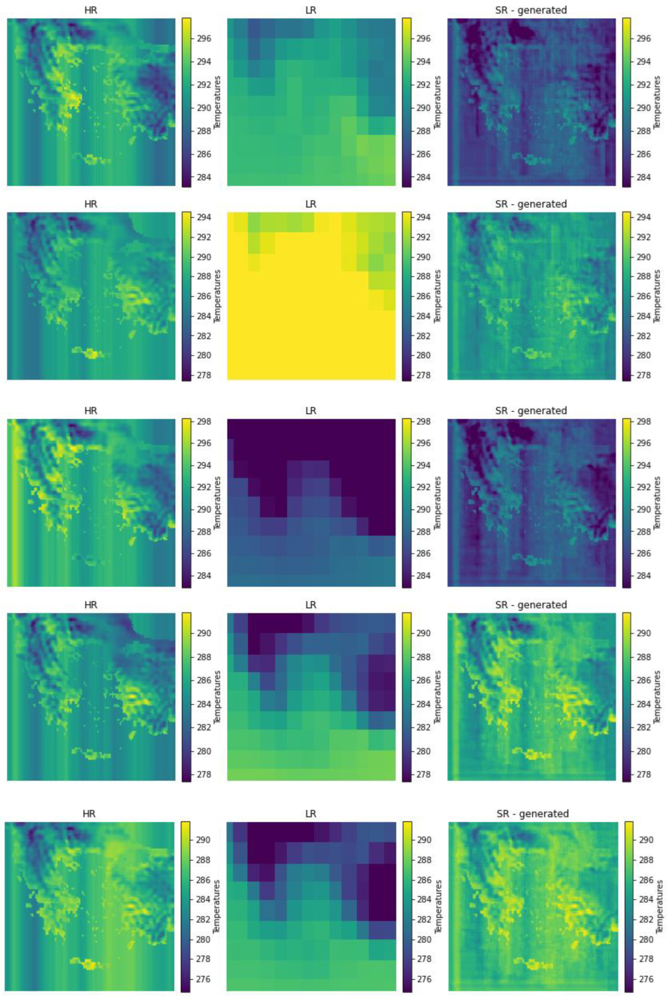
The high resolution data, after remapping each field to a 112x112 pixel grid, contains many nan temperature values over sea areas. In order to overcome this problem, the mean temperature of each column of the array was calculated and used to fill in the nans. That’s the reason behind the presence of some vertical lines in the original high resolution images of Figure 9.
The training data consists of low and high resolution images. Predictor-wise, the only data that were used originated from the Elevation parameter for training. For the training process, 80% of the previously described data were used and for validation and testing purposes the remaining 20% (15% for validation and 5% for testing respectively).
All images were scaled to [0, 1] prior feeding the generator and [-1, 1] prior feeding the discriminator. This was done because at the end of the generator network, the tanh activation layer is used which means that the feature maps values are now scaled to the range [-1, 1], so when feeding the discriminator network the high resolution images are scaled to [-1, 1].

Table 1.
Training data structural description.
| Dimensions | |
|---|---|
| Target resolution | time: 5124, lon: 112, lat: 112 |
| Coarse resolution | time: 5124, lon: 56, lat: 56 |
Training was done on a NVIDIA GeForce GTX 1650 with 4GB of memory and 896 cores lasted approximately 3 hours in order to complete 300 epochs. The batch size of the images was 8 and the learning rate was 1e-4 using the Adam optimizer.
2.4.2. Model Architecture—Metrics
For dealing with the task of downscaling to high resolution, a Deep Convolutional GAN (DCGAN) network architecture was implemented. In Figure 5, the generator’s architecture is depicted and in Figure 6 the discriminator’s architecture:
- The generator consists of downsampling and upsampling layers to produce high resolution images from low resolution images. It starts with a Dense layer that takes the low resolution image as input, then downsamples it by using two Conv2D layers, then upsamples it by using Conv2DTranspose layers until the desired image dimensions are reached. LeakyRelu was used as an activation function for all layers except for the last output layer which uses tanh.
- The discriminator consists of 5 Conv2D layers and one Dense layer. In each layer Relu is used as the activation function. Additional dropout layers were inserted after each Conv2D layer for preventing overfitting. The output layer uses sigmoid for the activation.
The role of the discriminator is to classify the image as low or high resolution and the generator progressively becomes better at creating realistic-looking high resolution images while the discriminator can no longer distinguish between high and low resolution images.
To quantify the quality of the generated images, the PNSR (Peak Signal to Noise Ratio) metric was used in this work to quantify the quality of the generated images. PSNR is a common metric used in the field of image processing and computer vision, including Generative Adversarial Networks (GANs), to evaluate the quality of reconstructed or generated images. PSNR is a measure of the peak error. It is calculated using the following formula:
where, is the maximum possible pixel value of the image and MSE is Mean Squared Error, calculated as:
where, I is an mxn image and K its noisy approximation.
3. Results
The objective evaluation of Generative Adversarial Networks remains an open problem. While there are several measures to be taken into consideration, there is no universal agreement on how to best capture and quantify the strengths and limitations of the models. Due to the complex nature of GANs and the nuances in their training, it’s often beneficial to use multiple methods to obtain a more holistic view of their performance.
3.1. Training
One of the simplest methods to achieve this is through the visual inspection of the generated samples, as seen in Figure 7. The generator progress during the 300 epochs in total can be seen in Figure 7. However, this is highly subjective and does not provide a quantitative measure of the quality.
To provide a quantification of the quality, the PNSR metric is provided in Figure 8. The higher the PSNR, the better the quality of the compressed or reconstructed image. In other words, a higher PSNR indicates that the reconstruction is of high quality. Conversely, a lower PSNR suggests poorer quality. As can be seen in Figure 8, the PSNR metric increases after each epoch, which is the desired effect.
Figure 9 depicts some of the predictions (generated images), from the test set that was split before the training took place. One of the findings of this study is that the addition of DEM as a predictor in the model has had the best performance in terms of both visual inspection and PNSR, when compared to predictors including land cover and soil type data.
In Figure 9, the DEM has improved the spatial distribution of temperatures across Greece. While this improvement is true when comparing to other model configurations tested, there seems to be an under and over estimation of temperatures in the predicted fields, especially in the mountainous areas. In coastlines the prediction is more challenging with both over/under estimation of temperature due to their complex sea-land interactions which are already a challenging case to predict.
Figure 9.
Real high-resolution images (left panel), coarse-resolution images (middle panel), generated downscaled images from the test set during training (right panel).
Figure 9.
Real high-resolution images (left panel), coarse-resolution images (middle panel), generated downscaled images from the test set during training (right panel).
3.2. Model Predictions
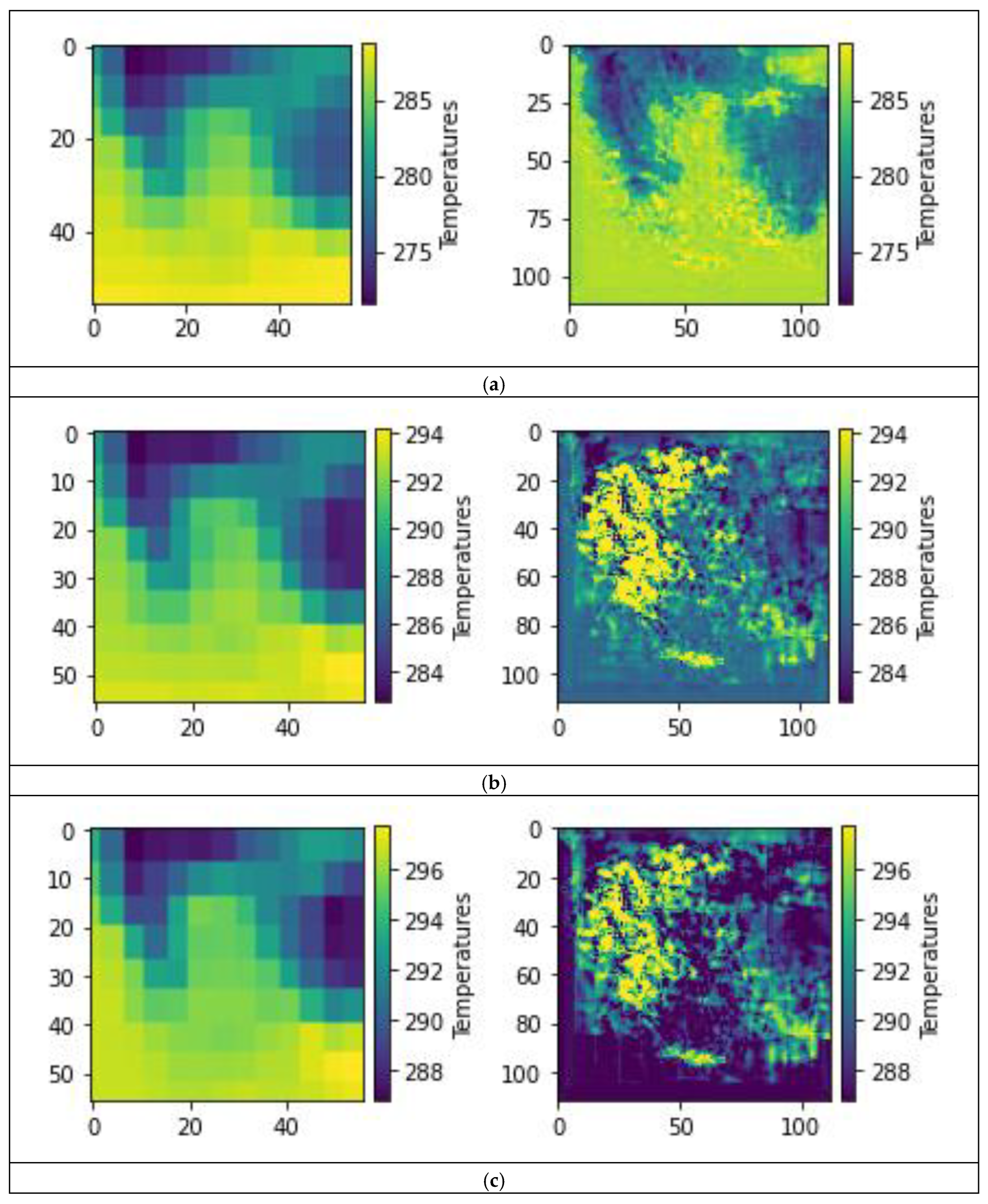
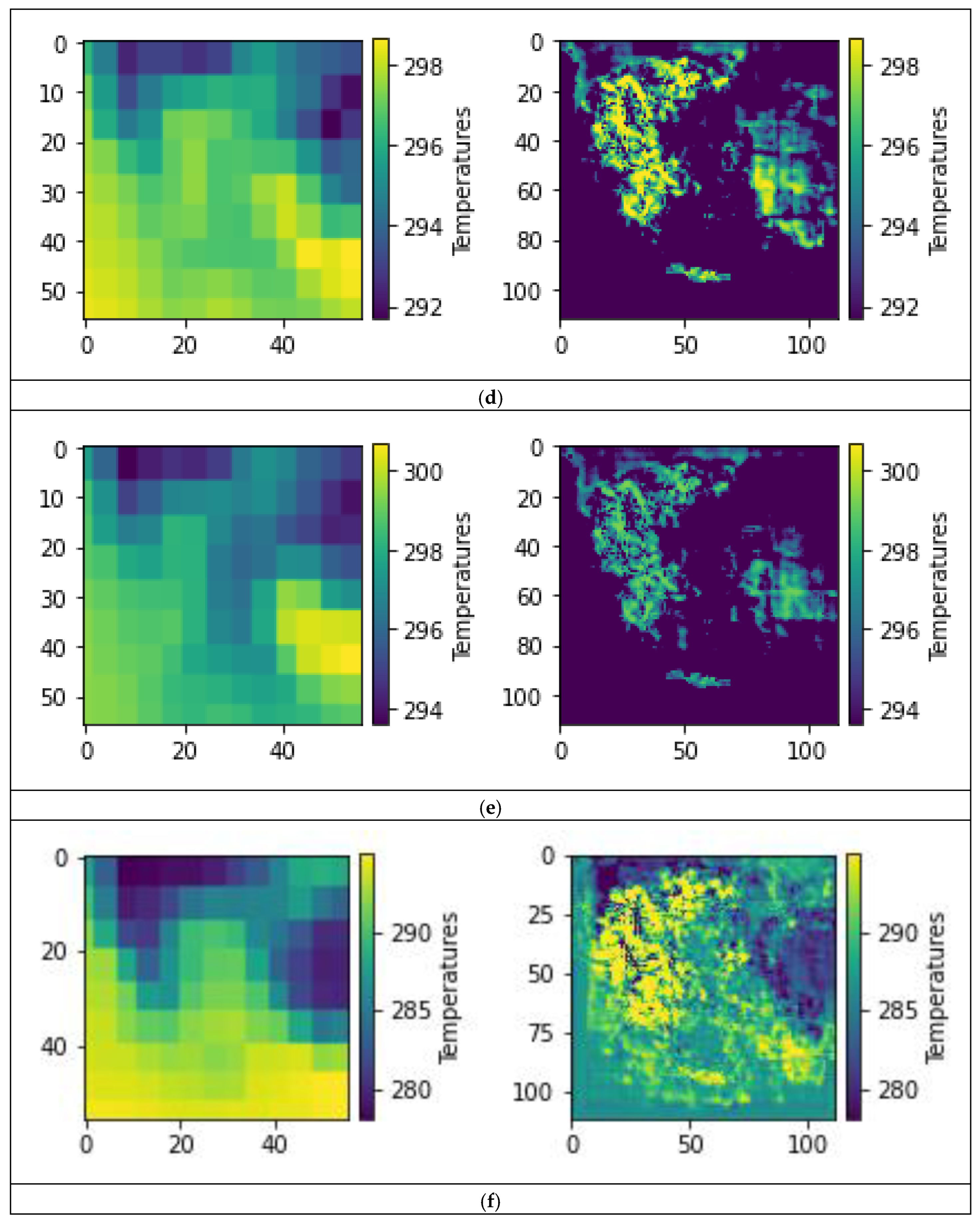
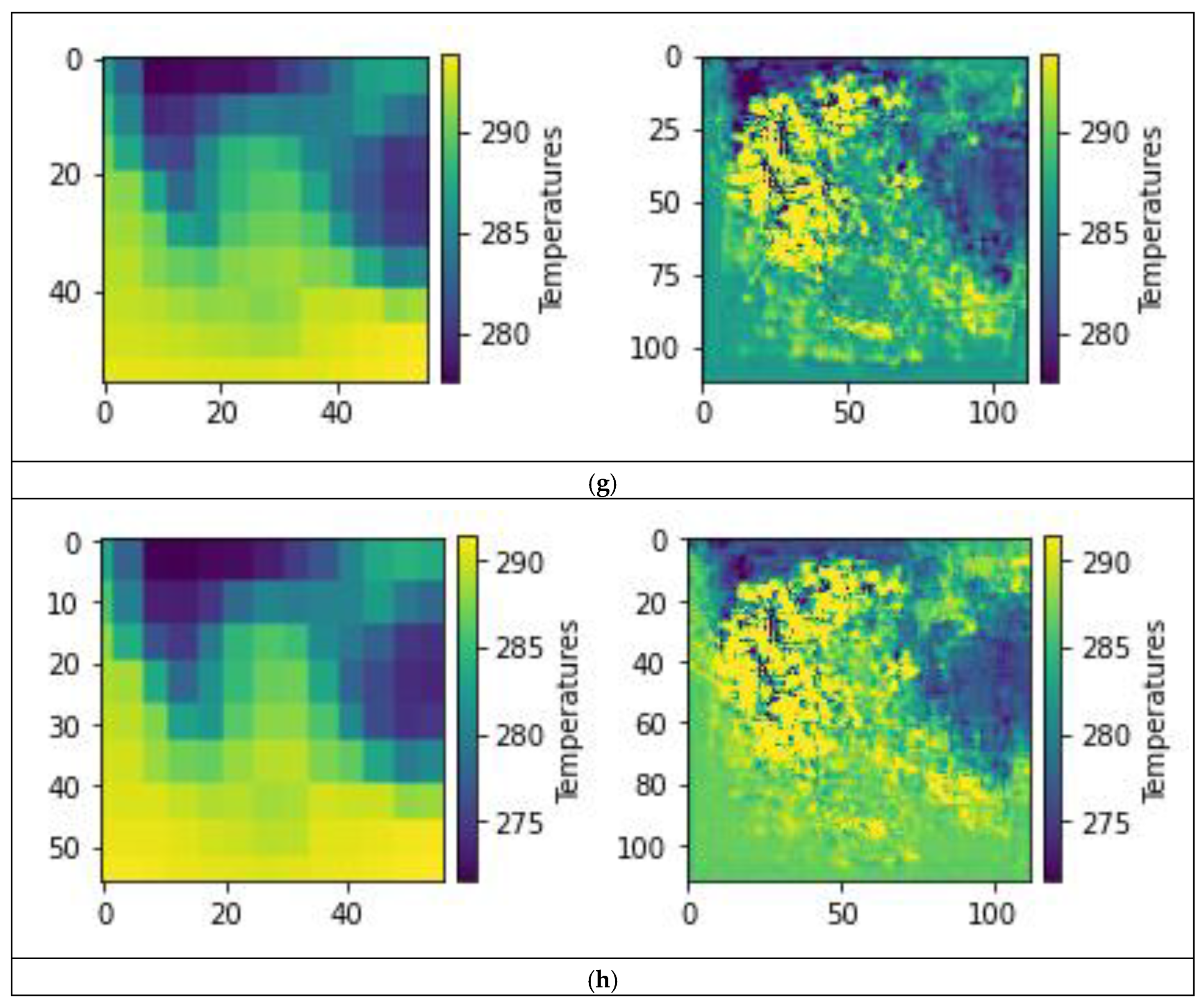
The trained model was finally tested using temperature forecasts outside of the training/test set for later dates (left panel) to generate the corresponding high-resolution predictions (right panel), as seen in Figure 10.
Figure 10, reveals that the model is able to translate the crude spatial resolution with higher granularity, following lower temperatures in mountainous regions with jumps in temperature difference in neighboring regions. This can be attributed to the complex topography represented by the DEM model. The spatial distribution seems to be in good agreement between predicted high resolution and coarse resolution in March (a) while during warmer months (b, c, d, e) we see an under prediction of temperatures especially over sea while values over mainland are over-predicted. During colder months (f, g, h), the model tends to overestimate the temperature, while capturing also a greater variability over sea. It must be noted that working with ERA5-Land data means the issue of missing data over sea had to be resolved while maintaining an adequate variability. This included using the mean temperature values per column of the array during data imputation instead of the mean values of the whole array.
4. Conclusions
In conclusion, the use of Generative Adversarial Networks (GANs) for downscaling meteorological fields has proven to be a promising and robust technique in meteorology [30,31]. The significant enhancement in resolution and accuracy, despite the inherent complexity and nonlinearity of meteorological fields, proves the power of these deep learning models [32]. These networks successfully address the spatial and temporal downscaling challenge by learning complex mappings between coarse and fine-scale data. The utility of GANs lies not only in the fine-scale output they can generate but also in their ability to maintain the temporal consistency and spatial coherence in the downscaled fields. This makes them highly useful for climate modeling, weather prediction, and other meteorological applications. The ability to learn and generate meteorological features that were previously not feasible with conventional downscaling methods demonstrates the superiority of GANs.
However, as with any sophisticated model, careful handling is needed. In a comprehensive assessment of Generative Adversarial Networks (GANs), it is evident that they demonstrate adequate performance in predicting spatial distributions of relevant meteorological fields. However, a notable shortcoming of GANs observed in this study lies in their limited precision in defining the ranges of the anticipated values, which raises the question of how this issue can be addressed. In the findings of this study, although various predictors were tested and included in the model, the inclusion of DEM was proven to provide the best quality images, although the generated fields were overestimated/underestimated in some cases. Potential solutions to enhance the accuracy may include, but are not limited to, extending the training period (assuming the corresponding datasets exist) or incorporating additional predictors, such as the Moderate Resolution Imaging Spectroradiometer (MODIS) land surface temperature, into the training dataset. Such approaches could refine the network’s capacity to produce more precise predictions. Despite these challenges, GANs hold considerable promise, offering advantages such as cost-effectiveness and decreased computational demands, once the network is trained for the defined area of interest [33]. Consequently, they are promising tools for achieving long-term, high-resolution predictions, potentially revolutionizing multiple sectors reliant on such detailed forecasting.
Uncertainty quantification remains a significant challenge and needs to be thoroughly addressed to fully leverage these models’ potentials. One should be aware of the potential pitfalls of overfitting that can arise within GAN frameworks. Also, GANs require decades of archives of high-quality data for training, which can often be a limiting factor in their application, especially if the end goal is to produce super-resolution predictions in the scale of meters.
Furthermore, the interpretability of GANs continues to be a challenge. While they have shown great promise in generating high-resolution meteorological fields, understanding why and how these models work is less clear. A deeper understanding of the internal mechanics of these models would enhance trust in their predictions and facilitate their broader adoption.
Despite these challenges, the future of GANs in the field of meteorological downscaling looks promising, provided that there is continued investment in model development, computational resources, and data availability. Ultimately, the evolution of these models will depend on the continued collaboration between the fields of meteorology, climate science, and machine learning [34]. The synergistic efforts between these domains have the potential to yield a significant breakthrough in our understanding and prediction of the Earth’s climate system.
Author Contributions
G.G contributed to the methodology, software, network architecture and validation, visualization, formal analysis, investigation, resources, writing of the original draft, review and editing. P.V contributed to methodology, formal analysis, investigation, researching, writing and preparing of the original draft, review and editing, effective supervision and funding acquisition. T.M contributed to data curation, visualization, investigation, writing of the original draft, review and editing. S.K contributed to methodology, formal analysis, investigation, review and editing, project administration, and funding acquisition. All authors have read and agreed to the published version of the manuscript. .
Funding
This study was funded by the European Union’s Horizon 2020 under reSilienT fARminG by Adaptive microclimaTe managEment (STARGATE) project (no. 818187).
Data Availability Statement
All of the data used in this study are available upon request.
Acknowledgments
The authors would like to acknowledge the European Union’s Horizon 2020 and STARGATE project for funding the work, the Copernicus Climate Data Store for providing the seasonal forecasts and ERA5-Land reanalysis data, as well as the Copernicus Land Monitoring Service for the providing the Elevation dataset used in this study.
Conflicts of Interest
The authors declare that they have no conflict of interest.
References
- Vitart, F., Robertson, A. W., Spring, A., Pinault, F., Roškar, R., Cao, W., ... & Zhou, S. Outcomes of the WMO Prize Challenge to Improve Subseasonal to Seasonal Predictions Using Artificial Intelligence. Bulletin of the American Meteorological Society 2022, 103(12), E2878–E2886.
- Robertson, A. W. , Vitart, F., & Camargo, S. J. (2020). Subseasonal to seasonal prediction of weather to climate with application to tropical cyclones. Journal of Geophysical Research: Atmospheres, 125(6), e2018JD029375.
- Mariotti, A. Mariotti, A., Baggett, C., Barnes, E. A., Becker, E., Butler, A., Collins, D. C., ... & Albers, J. Windows of opportunity for skillful forecasts subseasonal to seasonal and beyond. Bulletin of the American Meteorological Society 2020, 101(5), E608–E625. [Google Scholar]
- LeCun, Y. , Bengio, Y. & Hinton, G. Deep learning. Nature 521, 436–444 (2015). [CrossRef]
- Li, L. (2019). Geographically weighted machine learning and downscaling for high-resolution spatiotemporal estimations of wind speed. Remote Sensing, 11(11), 1378.
- Höhlein, K., Kern, M., Hewson, T., & Westermann, R. A comparative study of convolutional neural network models for wind field downscaling. Meteorological Applications 2020, 27(6), e1961.
- Sekiyama, T. T. (2020). Statistical downscaling of temperature distributions from the synoptic scale to the mesoscale using deep convolutional neural networks. arXiv preprint, arXiv:2007.10839.
- Leinonen, J. , Nerini, D., & Berne, A. (2020). Stochastic super-resolution for downscaling time-evolving atmospheric fields with a generative adversarial network. IEEE Transactions on Geoscience and Remote Sensing, 59(9), 7211-7223.
- Singh, A. , White, B., Albert, A., & Kashinath, K. (2020, January). Downscaling numerical weather models with GANs. In 100th American Meteorological Society Annual Meeting. AMS.
- Harris, L., McRae, A. T., Chantry, M., Dueben, P. D., & Palmer, T. N. A generative deep learning approach to stochastic downscaling of precipitation forecasts. Journal of Advances in Modeling Earth Systems 2022, 14(10), e2022MS003120.
- Scheiter, M., Valentine, A., & Sambridge, M. Upscaling and downscaling Monte Carlo ensembles with generative models. Geophysical Journal International 2022, 230(2), 916–931.
- Goodfellow, I. , Pouget-Abadie, J., Mirza, M., Xu, B., Warde-Farley, D., Ozair, S., Courville, A. & Bengio, Y., 2014. Generative adversarial nets, in Advances in Neural Information Processing Systems, Vol. 27, Curran Associates, Inc.
- Radford, A. , Metz, L. & Chintala, S., 2015. Unsupervised representation learning with deep convolutional generative adversarial networks, preprint (arXiv:1511.06434).
- Arjovsky, M., Chintala, S. & Bottou, L., 2017. Wasserstein generative adversarial networks. In Proceedings of the 34th International Conference on Machine Learning; PMLR; 70, pp. 214–223.
- Miralles, O., Steinfield, D., Martius, O., & Davison, A. C. (2022). Downscaling of Historical Wind Fields over Switzerland using Generative Adversarial Networks. Artificial Intelligence for the Earth Systems, 1-44.
- Winstral, A., T. Jonas, and N. Helbig, 2017: Statistical downscaling of gridded wind speed data using local topography. Journal of Hydrometeorology, 18 (2), 335–348.
- Nerini, D. , 2020: Probabilistic deep learning for postprocessing wind forecasts in complex terrain.
- Goodfellow, I., Y. Bengio, and A. Courville, 2016: Deep learning. MIT press.
- Vandal, T., E. Kodra, S. Ganguly, A. Michaelis, R. Nemani, and A. R. Ganguly, 2018: Generating high resolution climate change projections through single image super-resolution: An abridged version. Proceedings of the Twenty-Seventh International Joint Conference on Artificial Intelligence, 5389–5393. 5389. [Google Scholar] [CrossRef]
- Reichstein, M., G. Camps-Valls, B. Stevens, M. Jung, J. Denzler, N. Carvalhais, and Prabhat, 2019: Deep learning and process understanding for data-driven Earth system science. Nature, 566 (7743), 195–204. 7743. [Google Scholar] [CrossRef]
- Baño Medina, J., R. Manzanas, and J. M. Gutiérrez, 2020: Configuration and intercomparison of deep learning neural models for statistical downscaling. Geoscientific Model Development, 13 (4), 2109–2124. 2109. [Google Scholar] [CrossRef]
- Sha, Y., D. J. G. Ii, G. West, and R. Stull, 2020: Deep-Learning-Based Gridded Downscaling of Surface Meteorological Variables in Complex Terrain. Part I: Daily Maximum and Minimum 2-m Temperature. Journal of Applied Meteorology and Climatology, 59 (12), 2057–2073. [CrossRef]
- Höhlein, K., M. Kern, T. Hewson, and R. Westermann, 2020: A comparative study of convolutional neural network models for wind field downscaling. Meteorological Applications, 27 (6), e1961.
- Seasonal Forecasts Data Page on Climate Data Store. Available online: https://cds.climate.copernicus.eu/cdsapp#!/dataset/seasonal-original-single-levels?tab=overview (accessed on 30 May 2023).
- Schulzweida, Uwe. (2022). CDO User Guide (2.1.0). Zenodo. [CrossRef]
- ERA5-Land Data Page on Climate Data Store. Available online: https://cds.climate.copernicus.eu/cdsapp#!/dataset/reanalysis-era5-land?tab=overview (accessed on 30 May 2023).
- EU-DEM Data Page. Available online: https://land.copernicus.eu/imagery-in-situ/eu-dem/eu-dem-v1.1 (accessed on 30 May 2023).
- CORINE Land Cover Data Page. Available online: https://land.copernicus.eu/pan-european/corine-land-cover (accessed on 30 May 2023).
- Poggio, L. , de Sousa, L. M., Batjes, N. H., Heuvelink, G. B. M., Kempen, B., Ribeiro, E., and Rossiter, D.: SoilGrids 2.0: producing soil information for the globe with quantified spatial uncertainty, SOIL, 7, 217–240, 2021. https://soil.copernicus.org/articles/7/217/2021/.
- Saha, A. , & Ravela, S. (2022). Downscaling Extreme Rainfall Using Physical-Statistical Generative Adversarial Learning. arXiv preprint, arXiv:2212.01446.
- Price, I. , & Rasp, S. (2022, May). Increasing the accuracy and resolution of precipitation forecasts using deep generative models. In International conference on artificial intelligence and statistics (pp. 10555-10571). PMLR.
- Annau, N. J. , Cannon, A. J., & Monahan, A. H. (2023). Algorithmic Hallucinations of Near-Surface Winds: Statistical Downscaling with Generative Adversarial Networks to Convection-Permitting Scales. arXiv preprint, arXiv:2302.08720.
- Accarino, G., Chiarelli, M., Immorlano, F., Aloisi, V., Gatto, A., & Aloisio, G. (2021). MSG-GAN-SD: A Multi-Scale Gradients GAN for Statistical Downscaling of 2-Meter Temperature over the EURO-CORDEX Domain. AI 2021, 2, 600–620.
- Gong, B. , Ji, Y., Langguth, M., and Schultz, M. Statistical downscaling of precipitation with deep neural networks, EGU General Assembly 2023, Vienna, Austria, 24–28 Apr 2023, EGU23-10488. [CrossRef]
Figure 1.
General architecture of a Generative Adversarial Network.
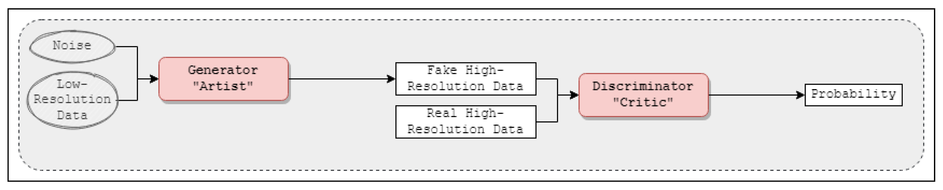
Figure 2.
Spatial distribution grid of seasonal temperature forecasts from ECMWF (in their raw format) covering the Hellenic domain.
Figure 2.
Spatial distribution grid of seasonal temperature forecasts from ECMWF (in their raw format) covering the Hellenic domain.
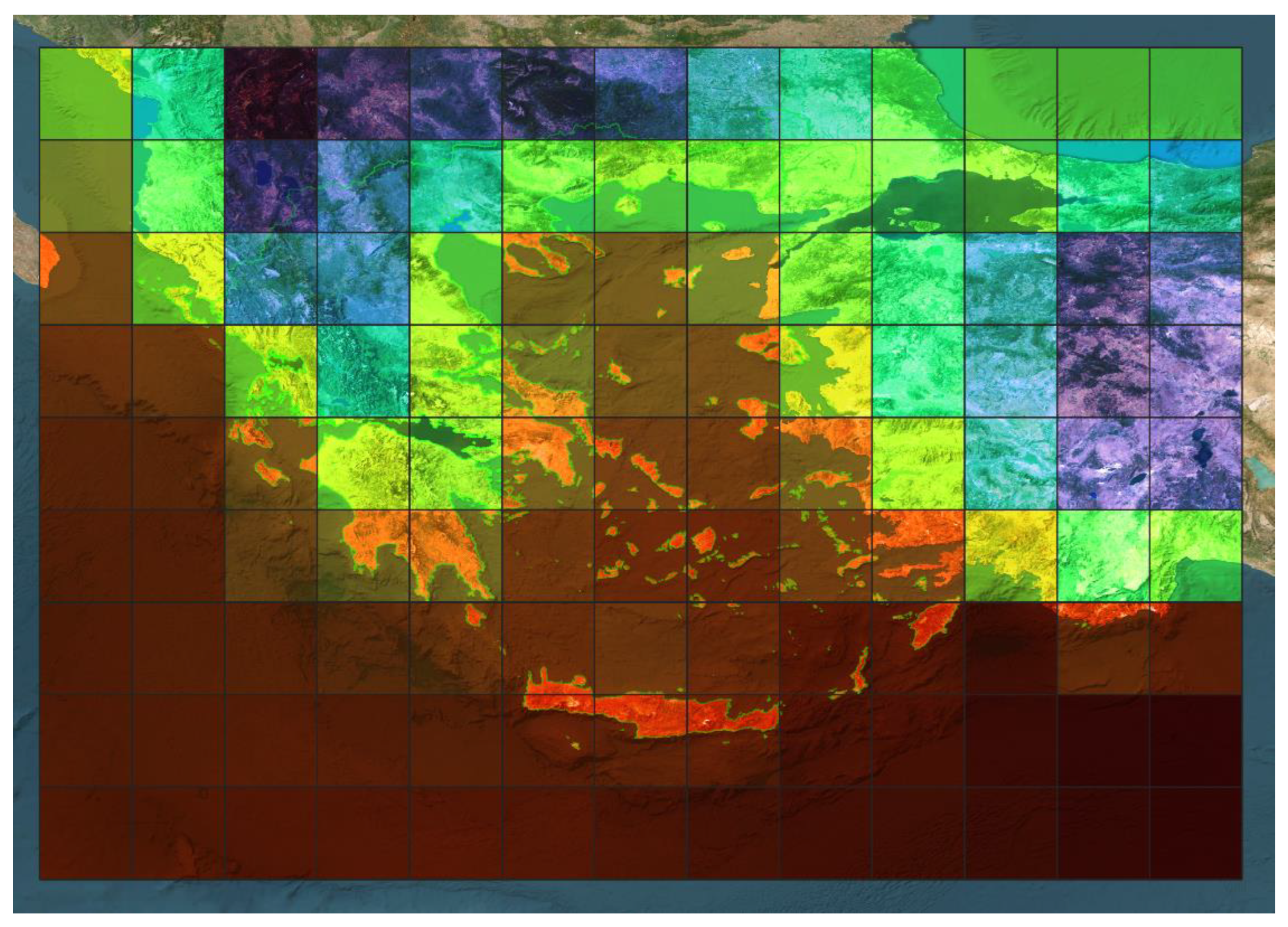
Figure 3.
Spatial distribution grid of reanalysis data ERA5-Land (in their raw format) covering the Hellenic domain.
Figure 3.
Spatial distribution grid of reanalysis data ERA5-Land (in their raw format) covering the Hellenic domain.
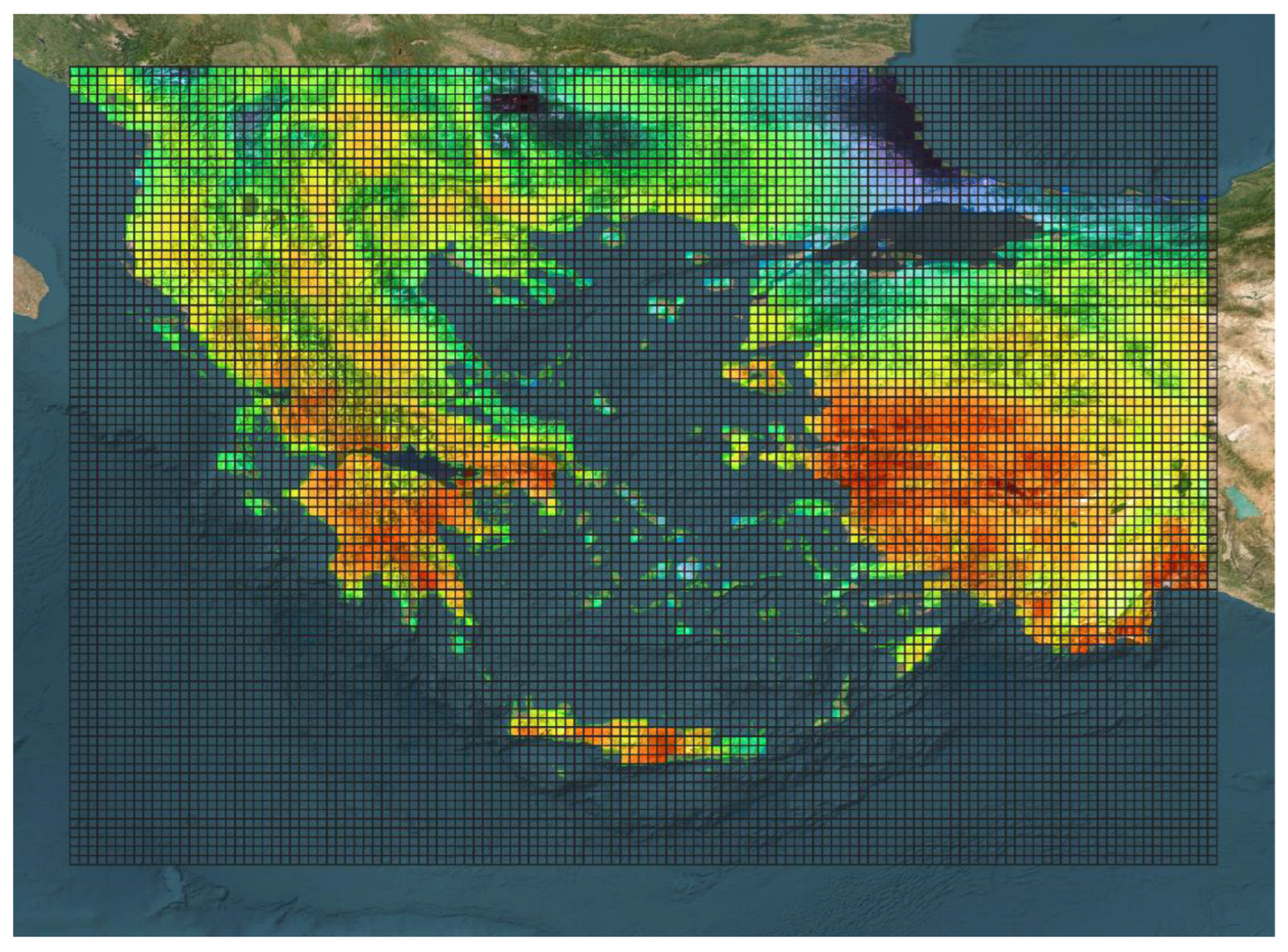
Figure 4.
Digital Elevation Model data covering the Hellenic domain.
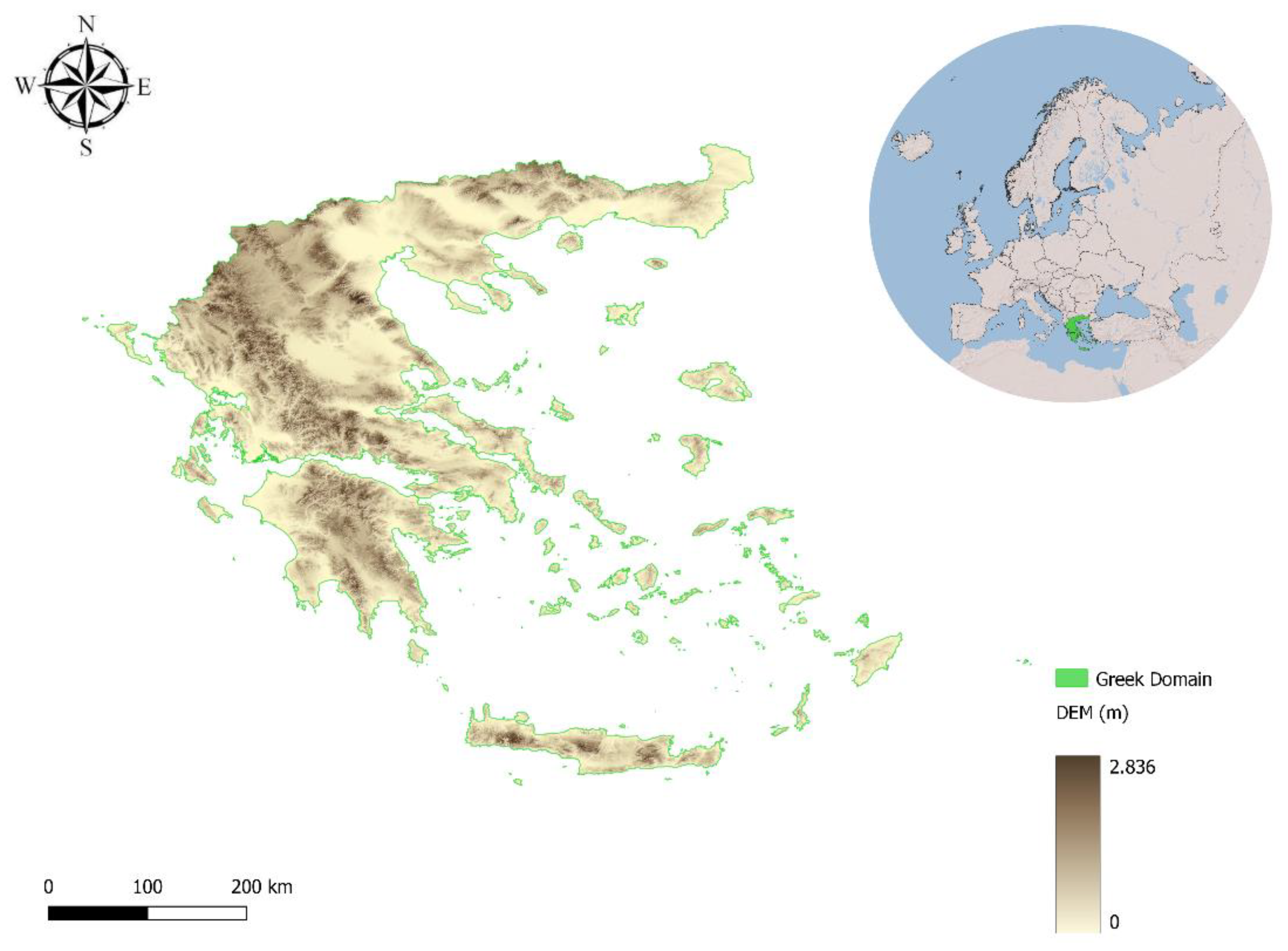
Figure 5.
Architecture of the generator network.

Figure 6.
Architecture of the discriminator network.

Figure 7.
Generator progress during training.
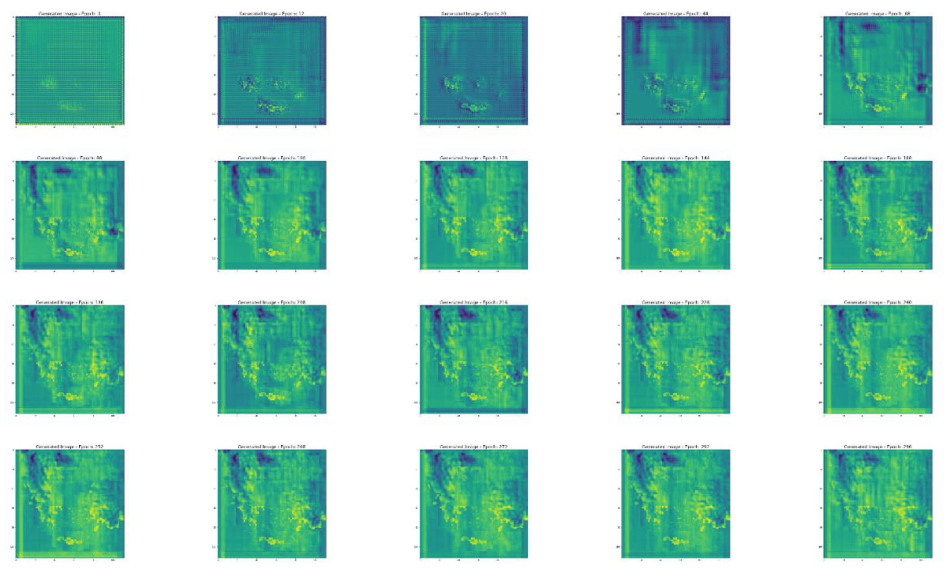
Figure 8.
PNSR metric.
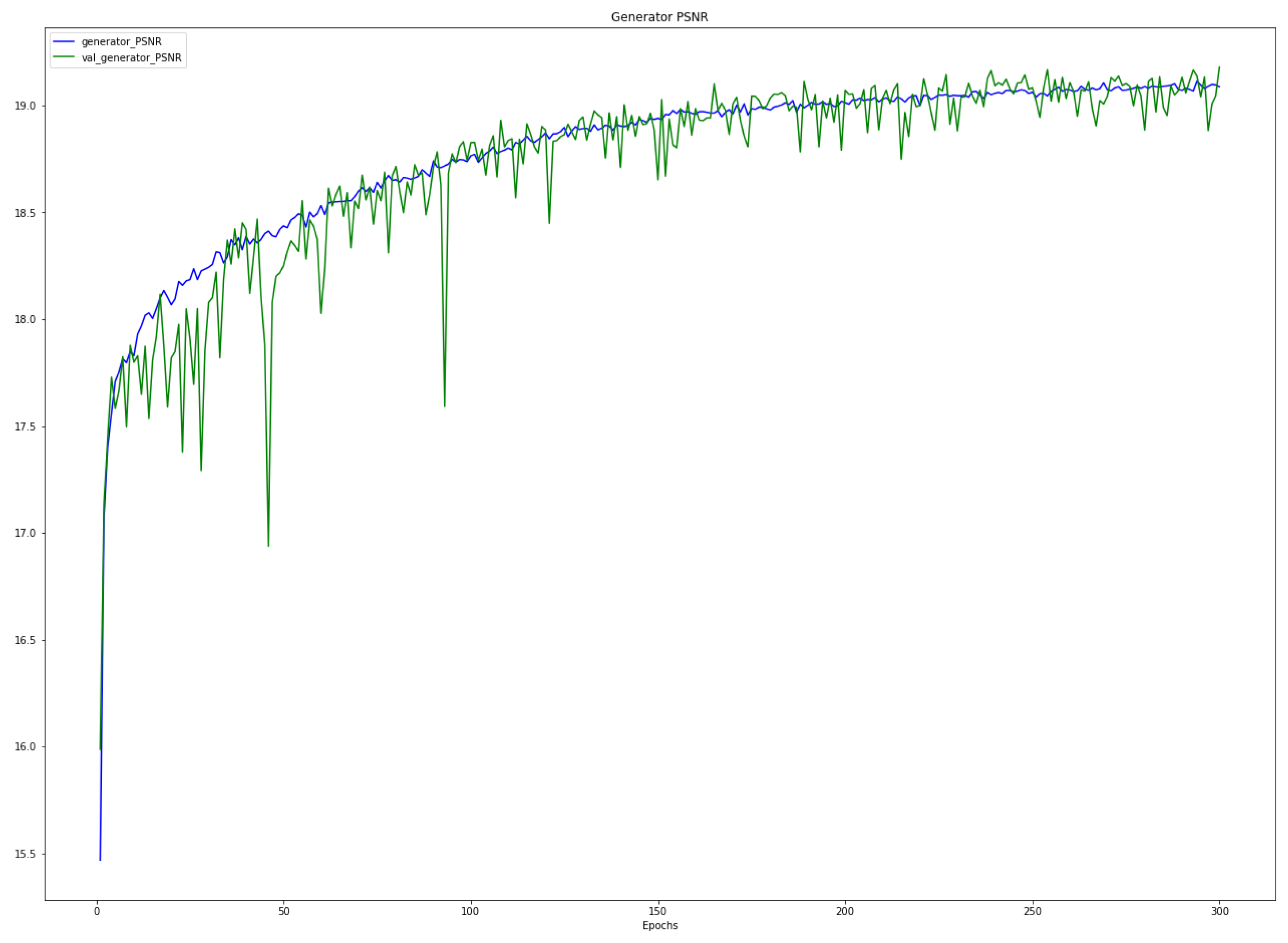
Figure 10.
Generated high-resolution temperature predictions (right panel) versus their original coarse counterparts (left panel) on: a) 2023-03-30, b) 2023-05-21, c) 2023-06-18, d) 2023-06-23, e) 2023-07-24, f) 2023-11-01, g) 2023-11-10, h) 2023-12-01.
Figure 10.
Generated high-resolution temperature predictions (right panel) versus their original coarse counterparts (left panel) on: a) 2023-03-30, b) 2023-05-21, c) 2023-06-18, d) 2023-06-23, e) 2023-07-24, f) 2023-11-01, g) 2023-11-10, h) 2023-12-01.
Disclaimer/Publisher’s Note: The statements, opinions and data contained in all publications are solely those of the individual author(s) and contributor(s) and not of MDPI and/or the editor(s). MDPI and/or the editor(s) disclaim responsibility for any injury to people or property resulting from any ideas, methods, instructions or products referred to in the content. |
© 2023 by the authors. Licensee MDPI, Basel, Switzerland. This article is an open access article distributed under the terms and conditions of the Creative Commons Attribution (CC BY) license (http://creativecommons.org/licenses/by/4.0/).
Copyright: This open access article is published under a Creative Commons CC BY 4.0 license, which permit the free download, distribution, and reuse, provided that the author and preprint are cited in any reuse.


