
Submitted:
21 June 2023
Posted:
21 June 2023
You are already at the latest version
Abstract
Wind power is one of the most important sources of renewable energy available today. A large part of the wind energy cost is due to the cost of maintaining wind power equipment. When a wind turbine component fails to function, it might need to be replaced under the less than ideal circumstances. This is known as corrective maintenance. To minimize unnecessary costs, a more active maintenance policy based on the life expectancy of the key components is preferred. Optimal scheduling of preventive maintenance activities requires advanced mathematical modeling. In this paper, an optimal preventive maintenance algorithm is designed using the renewal-reward theorem. In the multi-component setting, our approach involves a new idea of virtual maintenance which allows us to treat each replacement event as a renewal event even if some components are not replaced by new ones. The proposed optimization algorithm is applied to a four-component model of a wind turbine and the optimal maintenance plans are computed for various initial conditions. The modeling results showed clearly the benefit of PM planning compared to pure CM strategy (about 30% lower maintenance cost).
Keywords:
Algorithm design
; Combinatorial optimization
; Preventive maintenance
; Virtual maintenance
; Linear programming
; Wind turbine
; Weibull distribution
; Renewal-reward theorem
1. Introduction
Wind power technology is one of the most efficient sources of renewable energy available today [1]. A large part of the wind energy cost is due to the cost of maintaining wind power equipment (e.g. of the total lifecycle costs for offshore wind farms) [2]. A corrective maintenance (CM) of a turbine component, performed after a breakdown of the component, is usually more expensive than a preventive maintenance (PM) event, as some of the equipment is replaced in a planned manner. However, if PM activities are scheduled too frequently, the maintenance costs become unreasonably high, which entails the necessity of a maintenance schedule minimizing the expected replacement, logistic, and downtime costs.
There is a broad body of literature devoted to various optimization models of maintenance scheduling. Here we name just a few of the relevant papers that influenced our own approach. In the article by Lee and Cha [3], some general PM optimization models are presented. The effect of a PM action has been classified into three categories: failure rate reduction, the decrease of the deterioration speed, and age reduction. The paper concludes that it can be profitable to perform PM.
The article [4] looks at opportunistic maintenance which is a special kind of preventive maintenance. When one component breaks down, the maintenance personnel attending to the broken component might as well maintain other aged components to save some logistic costs. This is extremely beneficial for offshore wind farms, due to the large set-up costs.
In [5], optimization algorithms are developed to determine optimal PM schedules in repairable and maintainable systems. It was demonstrated that higher set-up costs make advantageous simultaneous PM activities. However, the suggested models are nonlinear, which means they are computationally hard to solve.
Our paper suggests a new optimization algorithm aiming at a PM plan , see Section 6, which proposes the next time for the replacement of one or several components at a minimal maintenance cost estimated for the whole planning time period , subject to certain linear constraints on . Here T is the life length of the wind turbine, is the starting time of the planning period, and is the vector of component ages at time s.
The age dynamics of our algorithm are based on the discrete Weibull distribution, see [6]. To account for the component deterioration due to aging, we assume that the PM cost increases as a linear function of the component’s age at the replacement moment. Previously, the PM replacement cost was usually treated as an age-independent constant, see for example [7,8]. Our approach focussing on age-dependence should be compared to that of [9], where the maintenance cost is assumed to depend on the total damage. Another relevant paper [10], quantifies the maintenance cost of a component using the reliability distribution.
Our definition of the objective function requires an application of the classical renewal-reward theorem, see for example [11]. This approach is quite straightforward in the one component case as explained in Section 2. In the multiple component case, however, when the true renewal events (all components are replaced simultaneously) are rarely encountered, our approach requires some kind of pseudo-renewal events. To this end, in Section 5 we introduce the key idea of the virtual maintenance replacement cost for a generic component having age a at time t.
Section 7 presents two sensitivity analyses and two case studies treating a four-component model of the wind power turbine. In particular, it was demonstrated that under the additional assumptions of [7], the new model produces similar results to those obtained in [7] but at a higher computational speed. Some technical proofs of our claims are postponed until the end of the paper.
2. A single component model
We start our exposition of the model by turning to the one-component case. Without planned PM activities, the maintenance cost flow is described by line 1 of Figure 1.
Here, the consecutive failure times (depicted by crosses) form a renewal process with independent inter-arrival times each having the same Weibull distribution W. After each failure, the broken component is replaced by a new one and the incurred replacement cost is g. According to the classical renewal-reward theorem, the long-term time-average reward (the maintenance cost in the current setting) is .
The lines 2-5 in Figure 1 introduce the renewal-reward model used to compute the time-average maintenance cost based on the PM planning strategy: plan the next PM replacement at time t after each replacement. Line 2 describes a scenario with the first failure occurring after the planned PM time and the first replacement is performed at time t, thereby the failure is avoided. The corresponding PM replacement cost is assumed to be a linear function of the component’s age at the time of a PM replacement.
According to line 3, after the PM replacement was performed at the cost , the next failure occurred before the next PM planned time . As a consequence, the second replacement was performed in a CM regime incurring the cost g, see line 4. The line 4 says that following the second replacement, the next PM is planned at time , that is at time t after the failure time . According to the placement of a cross on the line 4, we see on line 5 that the third replacement is performed in the PM regime and the next PM time is scheduled at time .
Recall that a random variable L has a Weibull distribution W if
where is a scale parameter and is a shape parameter of W. The mean value of L
is computed using the gamma function. The age dependence in the continuous time setting is best viewed in terms of the hazard function , telling how fast the failure rate increases with the component’s age t. In this paper, we use the discrete-time version of the Weibull distribution
so that
Using these expressions and the renewal-reward theorem we arrive at the following explicit formula involving the key parameters of the one component model . The proof of this result (as well as the forthcoming Proposition 3) is given in the end of the paper.
Proposition 1.
Think of an infinite planning horizon and a recurrent strategy of planning the next PM at time t after each replacement event. Then the time-average maintenance cost is the following function
of the planning time t.
(As a check one can send t to infinity and observe that this results in , the average maintenance cost in the absence of PM activities.)
Minimizing the function over the possible planning times t, produces a constant
which we will treat as the long-term maintenance cost per unit of time for the component in question. Notice that according to this formula, c is independent of the planning period .
3. Optimal maintenance algorithm in the one component case
In this section, we propose an optimization algorithm for PM scheduling during a discrete-time interval
assuming that at time s the component in use is of age a. If , we say that at the beginning of the planning period, the component was as good as new. This will allow us to find an optimal time for the next PM by minimizing the total maintenance cost during the whole planning period.
Definition 2.
For the one component model with a planning period , we call aPM planany vector
with binary components satisfying a linear constraint
For the given planning period , we define the total maintenance cost as a function of the planning time t for the next PM and the failure time u of the component in use. For , put
or using indicator functions,
Put also
This formula recognizes two possible outcomes:
- if , then the breakdown happens before the planned PM time, and the expected total maintenance cost is estimated to be , with c given by (1),
- if , so that there is no breakdown before the planned PM time, then the expected total maintenance cost is estimated to be
If at the starting time s of the planning period, the component in use has age , we will use a special notation for the first failure time, where
is defined in terms of the full life length L of a genetic component. If L has a discrete W distribution, then
Putting into the formula for , we arrive at a random variable
that gives us the total maintenance cost of the PM plan . Averaging over , we obtain the objective function
as the expected maintenance cost of the PM plans . Now we are ready to define the optimal maintenance plan as the solution to the following optimization problem:
Let be the PM time proposed by the solution of the minimization problem above, and notice that
The following proposition states a consistency property for the set of optimal times , providing with intuitive support for the suggested approach.
Proposition 3.
Suppose for some positive δ,
If , then
4. Multiple component model
In this section, we expand our one-component model to the component case. We now think of a wind turbine consisting of n components with j-th component having a life length distributed according to a Weibull distribution W, where parameters may differ for different . We will assume that components may require different replacement costs:
- the shared logistic and downtime costs associated with a CM activity,
- the component-specific CM cost,
- the fixed logistic cost plus the downtime cost during a PM activity,
- the component specific PM replacement cost for j-th component at age t.
To be able to update the formula (1) of the minimal time-average maintenance cost, we would need to determine the times of total renewal of the system which are not readily available in the multiple component setting. For illustration turn to Figure 2 dealing with the case of components.
Even in the absence of PM activities, see line 1, it is clear that the classical renewal-reward theorem is not directly applicable. Our solution to this problem is to treat each replacement event as total renewal events, sometimes by performing opportunistic maintenance and in some cases, by increasing the cost function to reflect the future additional age-related replacement costs. This idea is illustrated by lines 2-5 in Figure 2.
Consider a strategy when the next PM activity is planned at time t after each replacement. Line 2 depicts a case when the second component is broken first and before the time t of the next PM. As shown by line 3, both components are replaced at the failure time and the next PM is planned at time . In this way, the time can be viewed as the total renewal time of the two-component system. The incurred replacement cost is
Since according to the line 3, both components break down after the planned time for the next PM, both components are replaced in the PM regime so that the incurred replacement cost is
Continuing in this way by replacing both components at each maintenance event, we arrive at a renewal-reward process described in the general setting as follows.
Assume that we start at time 0 with n new components and denote by
the time of the first failure. With independence, we have
Thus, if we plan our next PM at time t after each maintenance replacement, the first renewal time is with
and the corresponding reward value is computed as
where
is the subset of components that would be replaced at the first failure. The renewal-reward theorem allows us to express the time-average maintenance cost as an explicit function of the planning time t.
However, replacing all of the components at each maintenance event irrespectively of the ages of the components in use is definitely a suboptimal strategy. If at a maintenance event, some component j is in a working condition and its current age a is rather small, then it might be more beneficial to let it continue working. To still be able to use the renewal argument in such a case, we introduce the idea of a virtual replacement. We replace the previous naive formula for reward with a more sophisticated one
where
chooses the minimum between two age-specific costs: the preventive replacement cost and the virtual replacement cost, see Section 5. The renewal-reward theorem implies that the time-average maintenance cost is computed as the following function of the planning time t
where stands for . Now, after minimising over t we define the desired constant
5. Virtual replacement cost
Returning to the one component model and focusing on an arbitrary component j, observe that in this one component case, the model parameters are , , , , and . Using this set of parameters, we introduce the virtual replacement cost function as a function of the current time t and the current age a of the component in question.
Since is the total cost of the optimal PM-plan in the one component set. In terms of this cost function, the virtual replacement cost is defined by the difference
This difference evaluates the extra maintenance cost over the time period due to the component’s age a at the starting time t of the observation period. The larger is a, the higher is the expected maintenance cost. The function
will be treated as the long-term virtual replacement cost of the component of age a.
Proposition 4.
If , then and
In the above described manner we can define and for all .
6. Optimal maintenance algorithm for multi components
For the planning period , we call a PM plan in the multi-component setting any array , where
and all components are binary subject to the following linear constraints
The equality means that the plan suggests a PM replacement of j-th component at time t. On the other hand, the equality means that according to the plan, at least one of the components should be replaced at time t, this is guaranteed by constraint () (constraint (8a) allows for several components to be replaced at such a time t). The equality means that no PM is planned during the whole time period . This is guaranteed by constraint ().
Given the current ages of n components
the first failure time is , where
Putting
we first mention a naive formula for the cost assigned to a PM plan assuming that at each maintenance event all n components are replaced by the new ones. With
where c is given by (5), put
Here the last term describes the option of planning no PM activity. This formula should be modified to incorporate the virtual replacement costs:
where
Notice that the total cost function does not explicitly depend on . The role of becomes explicit through the following additional constraint
It says that if , that is if a PM for at least one component is scheduled at time t, then for each component j, there is a choice between two actions at time t: either perform a PM, so that and , or do not perform a PM and compensate for the current age of the component by increasing the cost function using the virtual replacement cost value (corresponds to and ).
The optimal maintenance plan is the solution to the linear optimization problem
7. Case studies
This section contains five computational studies with our algorithm applied to a four-component model of a wind power turbine described next. Table 1 lists the four components in question and summarises the basic values of the model parameters, where the suggested values of are taken from the paper [12].
The cost unit is , and the time unit is one month. In accordance with paper [13], the lifetime of the wind turbine is assumed to be 20 years so that . Other basic values of the model are
7.1. Sensitivity analysis 1
In this section, we focus on the generator component of the four-component model and have a closer look at the cost function of age a
for different values of the parameters, keeps unchanged the announced values for the other parameters of the model.
Figure 3 summarises the results of this sensitivity analysis. The blue line in Figure 3 describes the function of age for the baseline set of parameter values. For small values of the age variable a, the cost function grows in a concave manner and beyond some critical age takes the linear form .
The red line shows what happens if we reduce but keep the sum unchanged. We see that the initial concave part of the curve is the same but the critical age becomes larger.
The green line indicates a drop in the cost function in response to the lowering of the monthly value loss parameter . Finally, the black line shows the cost reduction caused by a smaller value of . The black, blue, and red straight lines have the same slope because of the shared parameter value .
7.2. Sensitivity analysis 2
One of the most crucial parameters of our model is m, the monthly value depreciation of a genetic component. In this section, we consider the one-component model taking the rotor component as an example. We study how the optimal time to perform the next PM increases as becomes larger. All other parameters are fixed at their primary values.
Recall the formula for the time-average maintenance cost in the one-component setting:
where t is the planning time for the next PM. Considered as a function of m, the average cost is a linear function as depicted on the right panel of Figure 4 for different values of the planning time t.
The left panel of Figure 4 reveals an interesting phenomenon: there exists a critical value of the parameter m, beyond which the optimal PM plan is to never perform a PM activity. Indeed, at the value , we observe a jump from optimal planning time up to which is equivalent to of no planned PM.
The sudden jump on the left panel graph is explained on the right panel by comparing for different values of t. The five straight lines compare with respect to different values of the parameter m. For , the minimal cost among the five options is given by . For , the minimal cost is given by . For , the minimal cost is given by . It is also clear that starting for all the horizontal line, corresponding to , is always giving the minimal cost.
7.3. Sensitivity analysis 3
In this section, we illustrate the relation (7) for the one component (rotor). Figure 5 compares the optimal times for different starting times s of the planning period.
The curves confirm the stated relation . They also emphasize that for s closer to T, the approximation of the maintenance costs in (3) becomes rather hoarse for our model to give a reasonable answer. A recent paper [14] proposes an optimization model with special attention to the planning period near the end time T.
However, relation (7) allows an effective time effective implementation of our algorithm as a key ingredient of an app (for s not too close to T) by pre-calculating the constants .
7.4. Case study 1
This section deals with the full model of four components. The results for different initial ages of four components are shown in Table 2.
Comparing the first two cases, we find that , in accordance with Proposition 2. The two rightmost columns compare monthly maintenance costs for PM planning and pure CM strategy (no PM planning). Note that the maintenance cost becomes larger if the components are older at the start. On the other hand, according to Table 2 the PM planning may save around 4000 US dollars per month compared to the pure CM strategy. (The pure CM monthly costs are obtained by choosing a parameter m value so high that it is never beneficial to plan a PM activity.)
7.5. Case study 2
Here the optimization model developed in this paper is compared with the NextPM model from paper [7]. To adapt to the assumption of age-independent PM costs of paper [7], we set for all j. Put , , , , and for the values considered in paper [7].
The following three tables juxtapose the results produced by the two methods:
| 1 | 2 | 3 | 4 | Monthly maintenance cost | Matlab | |
| NextPM | x | x | 43 | x | 4.731 | 49 sec |
| New model | x | x | 43 | x | 4.703 | 2 sec |
| 1 | 2 | 3 | 4 | Monthly maintenance cost | Matlab | |
| NextPM | 50 | 50 | 50 | 50 | 4.964 | 54 sec |
| New model | 51 | 51 | 51 | 51 | 4.881 | 2 sec |
| 1 | 2 | 3 | 4 | Monthly maintenance cost | Matlab | |
| NextPM | 52 | 52 | 52 | 52 | 5.061 | 55 sec |
| New model | 52 | 52 | 52 | 52 | 5.040 | 2 sec |
The optimal schedules are almost identical, demonstrating the accuracy of the new method. Importantly, the new model only requires Matlab to solve it, and the new algorithm is much faster than the previous one.
8. Proofs of propositions
Proof of Proposition 1
We will need the following result from the renewal theory, see for example [11]. Let
be independent and identically distributed pairs of possibly dependent random variables: are positive inter-arrival times and are associated rewards. Define the cumulative reward process by
where is the number of renewal events up to time u, that is if
According to the renewal-reward theorem, the per unit of time reward
converges almost surely.
Recall that the full maintenance cost of the gearbox due to a CM is g, and a similar cost for PM is , where a is the gearbox age at the replacement. Thus, if we plan our next PM for a new gearbox at time t after each renewal event, then the corresponding renewal-reward process has inter-arrival time with
and the reward with
Since
the renewal-reward theorem implies that the time-average maintenance cost is computed as the following function of the planning time t
Proof of Proposition 3
By the definition of we have
To prove the assertion, it is sufficient to verify that
for .
To derive (12), we will introduce special notation
and notice that for
or in other words,
On the other hand, we have similarly,
The key observation leading to (12) is that the difference
is independent of t. In view of this fact, it is clear that the earlier observed inequality
entails
which immediately implies (12).
Proof of Proposition 4
If , then according to (3)
and
where in the last line we use notation (10) and (11). Since by definition, , the obtained equality
implies that provided
and we conclude
Furthermore, we see that
which together with Proposition 3 yields (7).
It remains to prove that or equivalently,
Since
This finishes the proof of Proposition 4.
Author Contributions
Conceptualization, Q.Y.; methodology, Q.Y.; software, Q.Y.; validation, Q.Y.; formal analysis, Q.Y.; investigation, Q.Y.; writing—original draft preparation, Q.Y., and S.S.; writing—review and editing, Q.Y., and S.S.; supervision, S.S. and O.C.; project administration, S.S. and O.C.; funding acquisition, O.C. All authors have read and agreed to the published version of the manuscript.
Funding
This research was funded by the Swedish Wind Power Technology Centre at Chalmers, the Swedish Energy Agency and Västra Götalandsregionen.
Institutional Review Board Statement
Not applicable
Data Availability Statement
All data used to support the findings of this study are included within the article.
Conflicts of Interest
The authors declare no conflict of interest.
Abbreviations
The following abbreviations are used in this manuscript:
| CM | Corrective maintenance |
| PM | Preventive maintenance |
References
- Márquez, F.P.G.; Karyotakis, A.; Papaelias, M. Renewable energies: Business outlook 2050; Springer, 2018.
- Röckmann, C.; Lagerveld, S.; Stavenuiter, J. Operation and maintenance costs of offshore wind farms and potential multi-use platforms in the Dutch North Sea. Aquaculture Perspective of Multi-Use Sites in the Open Ocean: The Untapped Potential for Marine Resources in the Anthropocene.
- Lee, H.; Cha, J.H. New stochastic models for preventive maintenance and maintenance optimization. European Journal of Operational Research 2016, 255, 80–90. [Google Scholar] [CrossRef]
- Sarker, B.R.; Faiz, T.I. Minimizing maintenance cost for offshore wind turbines following multi-level opportunistic preventive strategy. Renewable Energy 2016, 85, 104–113. [Google Scholar] [CrossRef]
- Moghaddam, K.S.; Usher, J.S. Sensitivity analysis and comparison of algorithms in preventive maintenance and replacement scheduling optimization models. Computers & Industrial Engineering 2011, 61, 64–75. [Google Scholar]
- Guo, H.; Watson, S.; Tavner, P.; Xiang, J. Reliability analysis for wind turbines with incomplete failure data collected from after the date of initial installation. Reliability Engineering & System Safety 2009, 94, 1057–1063. [Google Scholar]
- Yu, Q.; Patriksson, M.; Sagitov, S. Optimal scheduling of the next preventive maintenance activity for a wind farm. Wind Energy Science 2021, 6, 949–959. [Google Scholar] [CrossRef]
- Santos, F.P.; Teixeira, Â.P.; Soares, C.G. Modeling, simulation and optimization of maintenance cost aspects on multi-unit systems by stochastic Petri nets with predicates. SIMULATION 2019, 95, 461–478. [Google Scholar] [CrossRef]
- Chen, Y.L. A bivariate optimal imperfect preventive maintenance policy for a used system with two-type shocks. Computers & Industrial Engineering 2012, 63, 1227–1234. [Google Scholar]
- Liu, B.; Xu, Z.; Xie, M.; Kuo, W. A value-based preventive maintenance policy for multi-component system with continuously degrading components. Reliability Engineering & System Safety 2014, 132, 83–89. [Google Scholar]
- Grimmett, G.S.; Stirzaker, D.R. Probability and random processes; Oxford university press, 2020.
- Tian, Z.; Jin, T.; Wu, B.; Ding, F. Condition based maintenance optimization for wind power generation systems under continuous monitoring. Renewable Energy 2011, 36, 1502–1509. [Google Scholar] [CrossRef]
- Ziegler, L.; Gonzalez, E.; Rubert, T.; Smolka, U.; Melero, J.J. Lifetime extension of onshore wind turbines: A review covering Germany, Spain, Denmark, and the UK. Renewable and Sustainable Energy Reviews 2018, 82, 1261–1271. [Google Scholar] [CrossRef]
- Yu, Q.; Strömberg, A.B. Mathematical optimization models for long-term maintenance scheduling of wind power systems. 2021, arXiv:math.OC/2105.06666. [Google Scholar]
Figure 1.
Renewal-reward model for computing c for the one component model.
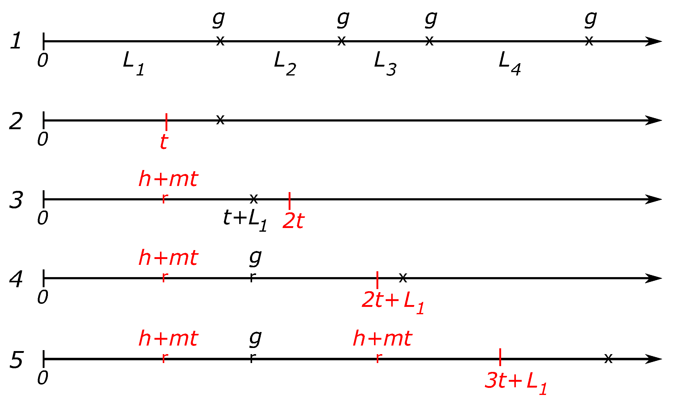
Figure 2.
Renewal-reward model for computing c for the two-component model.
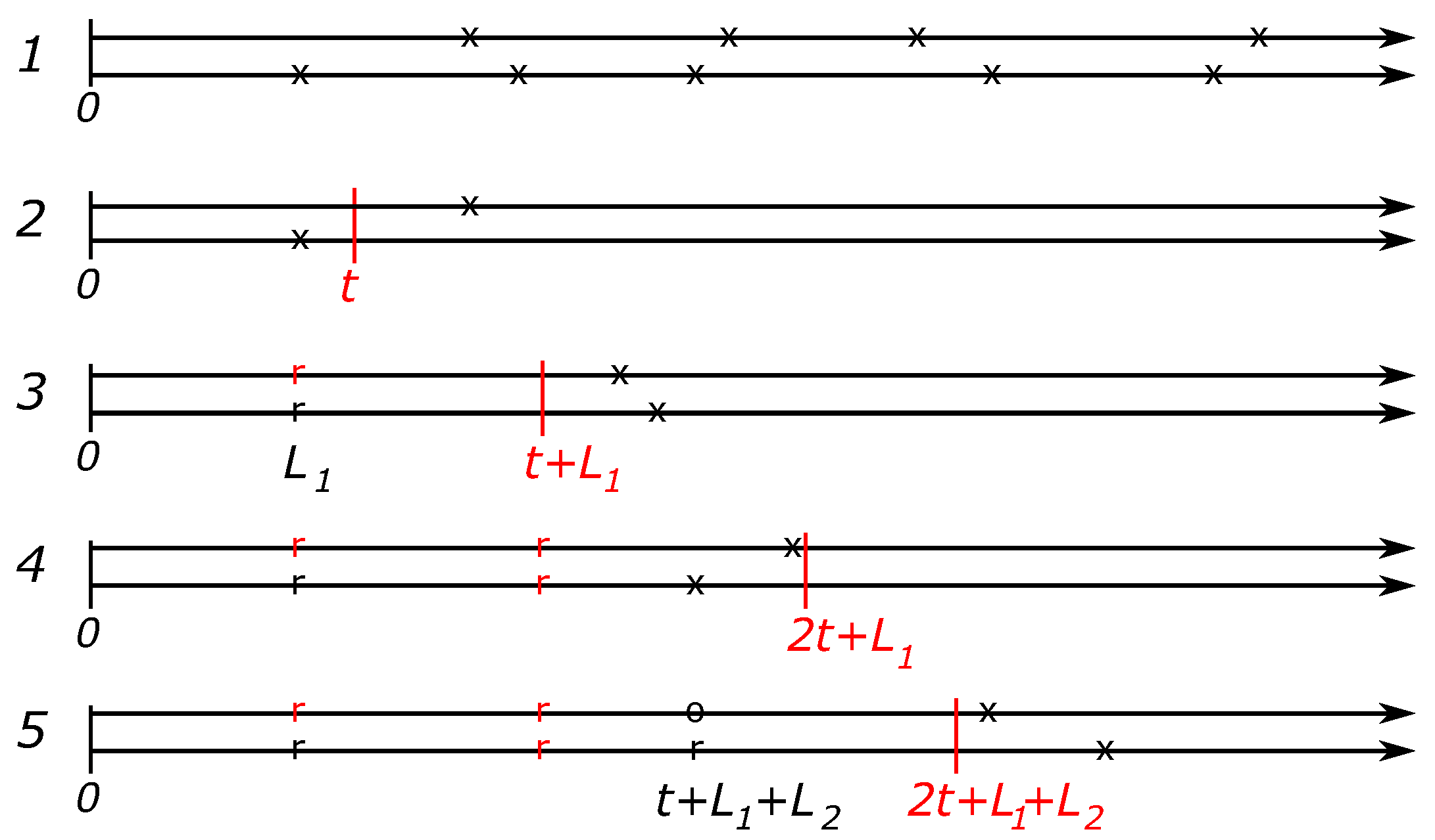
Figure 3.
Plots of for different combinations of parameters .
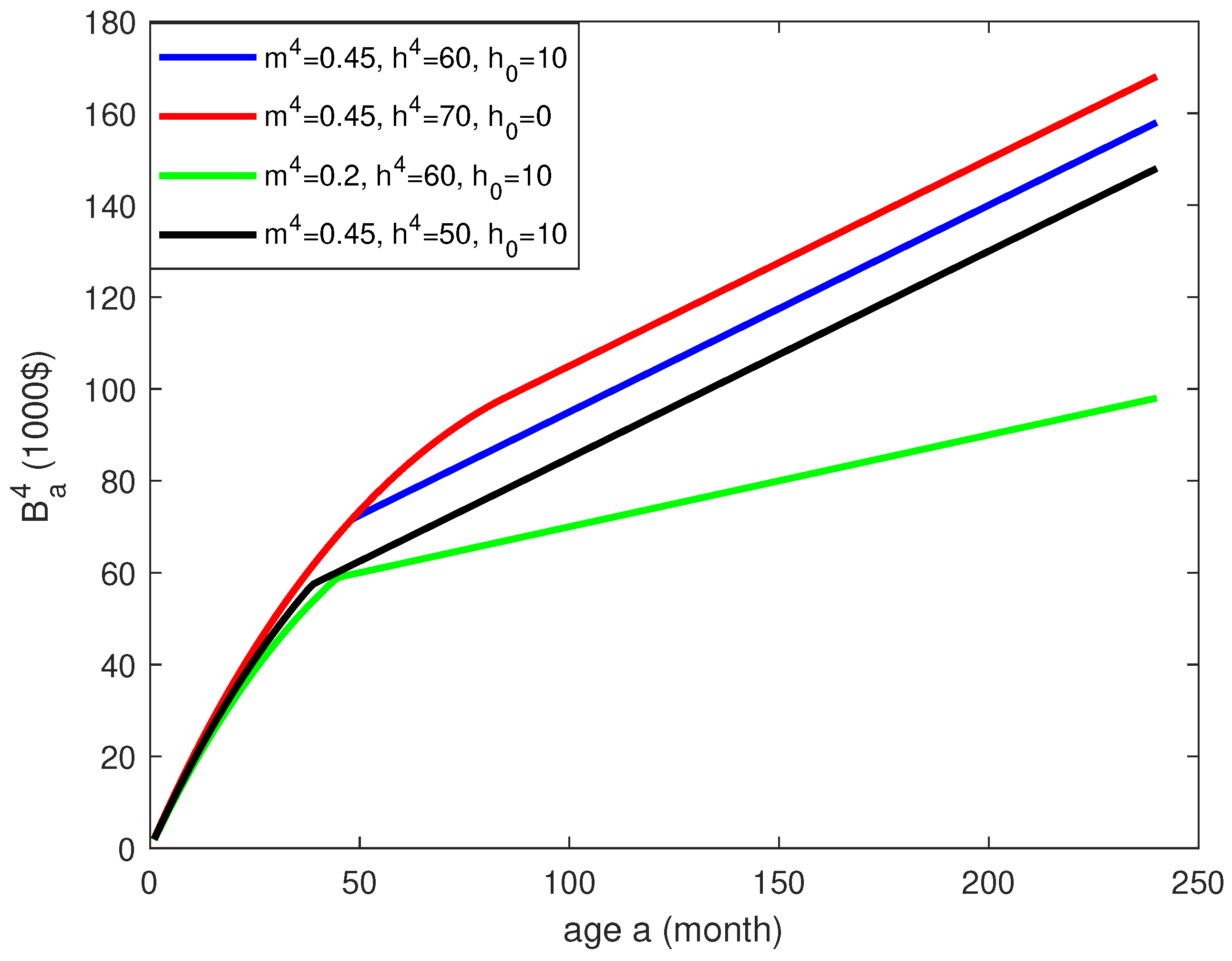
Figure 4.
Left panel: the optimal time to perform the next PM as a function of the parameter m. Right panel: different average cost based on different PM plans and different monthly value loss m.
Figure 4.
Left panel: the optimal time to perform the next PM as a function of the parameter m. Right panel: different average cost based on different PM plans and different monthly value loss m.
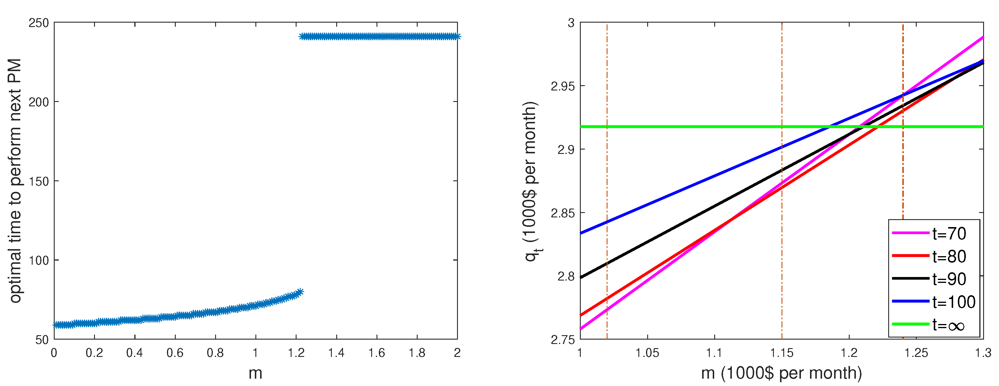
Figure 5.
Plots of for different s.
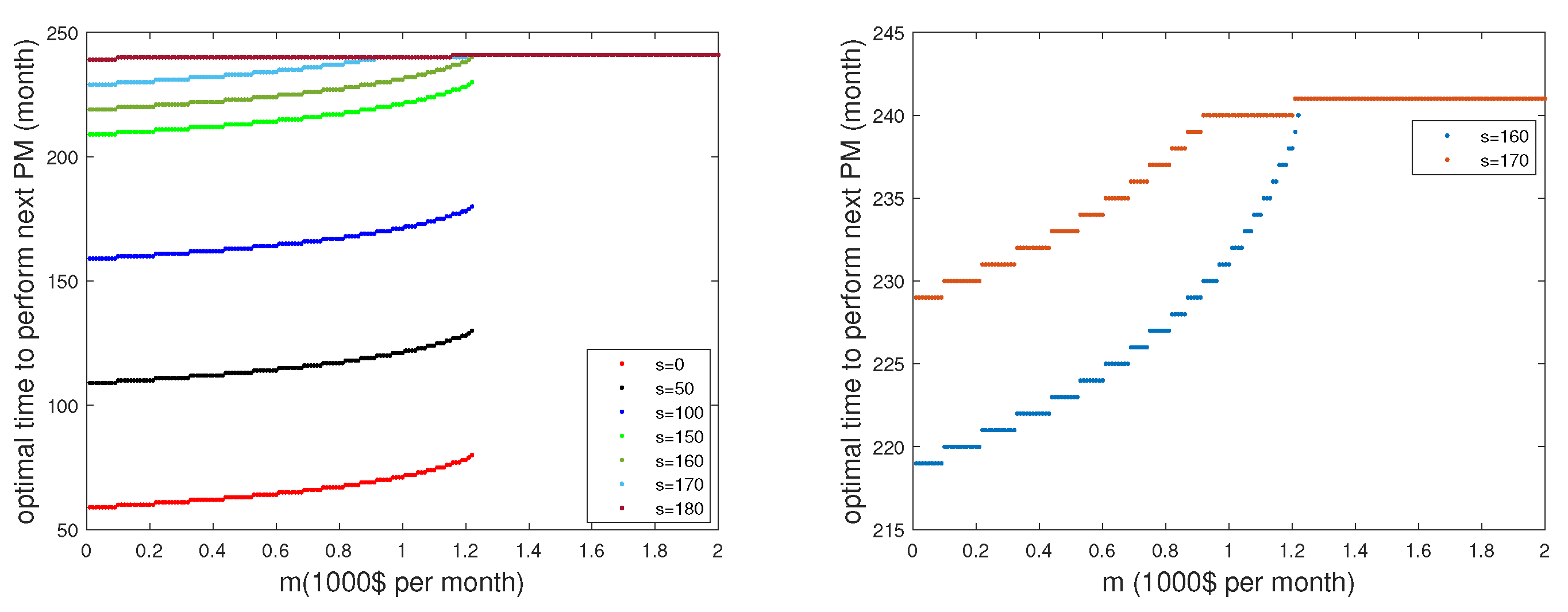

Table 1.
Base values for the component model.
| Component (j) |
, CM replacement cost |
, value loss per month |
Weibull shape |
Weibull scale |
|---|---|---|---|---|
| Rotor | 162 | 0.5 | 3 | 1e-06 |
| Main Bearing | 110 | 0.25 | 2 | 6.4e-05 |
| Gearbox | 202 | 1 | 3 | 1.95e-06 |
| Generator | 150 | 0.45 | 2 | 8.26e-05 |
Table 2.
The next PM plan for 4 components with different initial ages.
| Initial ages | PM | CM | ||||
|---|---|---|---|---|---|---|
| 62 | x | 62 | x | 9.937 | 13.756 | |
| 32 | x | 32 | x | 10.815 | 15.064 | |
| 46 | x | 46 | 46 | 10.469 | 14.868 | |
| 47 | 47 | 47 | 47 | 10.458 | 14.668 | |
| x | x | 12 | x | 10.364 | 14.229 |
Disclaimer/Publisher’s Note: The statements, opinions and data contained in all publications are solely those of the individual author(s) and contributor(s) and not of MDPI and/or the editor(s). MDPI and/or the editor(s) disclaim responsibility for any injury to people or property resulting from any ideas, methods, instructions or products referred to in the content. |
© 2023 by the authors. Licensee MDPI, Basel, Switzerland. This article is an open access article distributed under the terms and conditions of the Creative Commons Attribution (CC BY) license (http://creativecommons.org/licenses/by/4.0/).
Copyright: This open access article is published under a Creative Commons CC BY 4.0 license, which permit the free download, distribution, and reuse, provided that the author and preprint are cited in any reuse.


