
Submitted:
20 June 2023
Posted:
21 June 2023
You are already at the latest version
Abstract
This study reports fractal analysis of one-year radon in groundwater disturbances from five stations in China amid the catastrophic Wenchuan (Mw=7.9) earthquake of May 12, 2008 (day 133). Five techniques are used (DFA, fractal dimensions with Higuchi, Katz, Sevcik methods, power-law analysis) in segmented portions glided throughout each signal. Noteworthy fractal areas are outlined in the KDS, GS, MSS station data, while the portions were non-significant for PZHS and SPS. Up to day 133 critical epoch DFA-exponents have 1.5<=a<2.0 with several above 1.8. Fractal dimensions exhibit Katz’s D around 1.0-1.2, Higuchi’s D between 1.5-2.0 and Sevcik’s D between 1.0-1.5. Several power-law exponents are above 1.7 and numerous above 2.0. All fractal results of KDS-GS-MSS stations are further analysed using a novel computerised methodology which locates the exact out-of-threshold fractal areas and combines the outcomes of different methods per five, four, three, and two (maximum 13 combinations) versus nineteen Mw<=5.5 earthquakes of the area. Most different-technique coincidences are before the great Wenchuan earthquake and its post-earthquakes. This is not only with one method, but with 13 different methods. Other interpretations are also discussed.
Keywords:
DFA
; fractal dimension
; Katz
; Higuchi
; Sevcik
; spectral fractal analysis
; radon in groundwater
; earthquakes
1. Introduction
When it comes to severe natural disasters, earthquakes stand out since they may result in great loss of lives and property. Residents of large cities may experience severe effects from the massive quantity of energy produced during an earthquake, especially if the earthquake’s core is nearby. Catastrophic earthquakes are unavoidable as natural occurrences but highly challenging to foresee [1]. Consequently, the hunt for trustworthy seismic precursors is one of science’s greatest difficulties, and significant efforts have been done for many years in this area [2,3,4,5,6,7,8,9] The issue of earthquake prediction is still open, though [10]. Earthquakes are inherently complex, thus, several techniques and multi-level strategies are required [7]. In regions where severe earthquakes are possible, the associated prediction calls for the gradual downscaling of time, location, and magnitudes [2]. Along with the electromagnetic disturbances in the ULF, LF, HF, and VHF frequencies which indicate approaching earthquakes [4,9], radon-222 (hereafter radon) is a long-established precursor of impending seismic activity [2,7,11] . Radon is an inert gas created by the radioactive decay of the 238U series with a half-life of 3.86 days. When it disintegrates, it dissolves in the soil’s pores and liquids before moving on to surface, subsurface water and atmosphere. It is because that radon can travel to short and long distances in water and soil, and may be found at detectable quantities far from its generation location, that made it very significant in earthquake related studies [1]. As the above reviews mention [2,7,11], there is a great number of papers reporting pre-seismic changes of radon in groundwater, soil gas, atmosphere, wells and thermal spas. As a result, there is a substantial body of studies examining the relationship between radon emission and earthquake activity [10]. One of the key components of the present research is the abnormal behaviour of groundwater radon as a result of the catastrophic Wenchuan (=7.9) shallow (depth=19 ) earthquake occurred on May 12, 2008 (calendar’s day - hereafter - 133), along the Longmenshan fault (31.0°N, 103.4°E) at Sichuan Province, China [12,13] (Figure 1)). This quake was the most destructive one of China since 1976 and the second most devastating seismic shock of this century after the great Sumatra earthquake in 2004 [14]. The groundwater data consists of one-year measurements received from China between 1 January 2018 and 31 December, 2008 by five different stations (Figure 2) between 105.6 and 526.0 from the earthquake’s epicentre (Table 1) a possible connection between the variability of geochemical signals and the Wenchuan-induced seismicity can provide insight into the associated underlying processes since the data include information about the subsurface dynamics. The Detrended Fluctuation Analysis (DFA), the use of fractal dimension (FD) with different methodologies and the power-law fractal analysis are very robust and reliable fractal methods [1,15,16,16]. Importantly, the fractal methods can recognise underlying scaling and long-range features that are characteristic for the unavoidable occurrence of earthquakes even in noisy and non-stationary time series.
2. Materials and methods
2.1. Experimental aspects
2.1.1. Earthquake activity
The Wenchuan earthquake occurred on the Longmenshan fault (LMSF), which is parallel to eastern Tibet and the Sichuan basin in the northeast and southwest directions (Figure 1) and is about 500 long and 40-50 broad [17]. According to Liu et al.[12], the Wenchuan-Maowen, Yingxiu-Beichuan and Guanxian-Jiangyou faults, as well as a number of thrust faults produced by the compression of the eastern Tibetan Plateau and the Yangtze craton, dominate the LMSF zone. Only one significant seismic event (=6.1) occurred in the LMSF zone before the Wenchuan earthquake, and that was in 1989 [17]. The LMSF zone was dormant until 2008 [12]. The 290 long segment of the LMSF that was ruptured by the Wenchuan earthquake propagated independently 270 in the NE and 20 in the SW direction. The co-seismic surface rupture was 80 . According to Liu et al. [12], the Wenchuan earthquake was caused by a shift in the LMSF’s dip angle (30° -50°SW to 60°-70°NE) and fault motion (SW thrusting motion to NE strike-slip motion). The Wenchuan earthquake disaster resulted in 69,225 fatalities, 374,640 injuries, 17,939 unaccounted-for persons, and over 5 million displaced people.
2.2. Measurement setup
Over the past 50 years, China has developed and established a structured network to track radon levels in groundwater for seismic studies. Almost all of China’ s provinces are represented in the network, which is made up of stations with a variety of instruments (Ren et al., 2012). The network is operated, maintained, and expanded with financial support from the China Earthquake Administration. The supplied radon series may be hourly (High Sampling Rate-HSR) or daily (Low Sampling Rate-LSR), depending on the sensors deployed at each station. Table 1 lists the LSR stations as Ganzi, Mingshan, Panzhihua and Sonpan, whereas the HSR station is only Kangding. To measure the amount of radon in groundwater, two instruments are used at China’s stations. Groundwater is sampled and degassed via bubbling at LSR stations. Then, using a specialised apparatus with the code FD-125, it is directed into an ion chamber or ZnS (Ag) detector where the concentration is determined by ionisations or scintillations. For the HSR Kangding station, groundwater is forced via a de-gasser and a gas-collecting device into a ZnS (Ag) detector, where radon is detected by a specialised instrument coded SD-3A with an hourly sample interval [18]. The accuracy for HSR and LSR measurements is 0.1 .
3. Mathematical Aspects
3.1. Fractal and long-memory
Numerous natural physical systems can be explained by fractals. The usual fractal behaviour is often seen when the system or a section of it is stretched, translated, or rotated in space. Depending on the mathematics explaining the changes, the related system is either self-affine or self-similar. Natural systems that are self-affine and self-similar are fractals in the sense that any component of them is a little or big copy of the total, but at various scales. As a consequence, fractal systems may be studied by focusing on its constituent parts. Additionally, the scaling characteristics of a fractal system are closely related to its long-memory [19,20,21,22] and complexity [20,23,24,25,26]. Because fractal behaviour, long-memory and complexity are interconnected concepts, examining one of them will usually result in the other. For example, examining a system’s long-memory will help define its complexity and vice versa [1,27,28]. All of these characteristics can show whether a system’s past, present, and future are strongly connected. The direct methods are effective for calculating a system’s fractal features [16,27]. The methods of Katz, Higuchi, and Sevcik are used in this paper because they offer direct estimates for fractal dimension computations [1,29]. Power-law dependencies are also present in fractal systems with long memory and complexity. DFA and spectral power-law analysis are useful tools for properly delineating these connections [1,27]. These techniques are used in this paper, as well, because of this. By use of the associated Hurst exponent, all approaches may be compared. These techniques are going to be thoroughly explained in the sections that follow. Hurst exponent is introduced first, followed by the robust DFA, the techniques for direct calculation of fractal dimension and finally, the power-law analysis.
3.2. Hurst exponent
A metric known as the Hurst exponent (H) may be used to identify long-lasting connections in both time and space [30,31]. The roughness of the associated time series may be evaluated while time-evolving fractal phenomena can be identified using the Hurst exponent [1,32,33]. The Hurst exponent has been used in a variety of research topics, including hydrological applications [30,31], astrophysical applications [34,35], processes of capital markets [36,37,38,39], noisy observations of traces in traffic [40,41,42], seizures prior to epilepsy [43,44,45] climatic dynamics [46] and precursory time series before impending earthquakes [1,7,8,47] The Hurst exponent value offers important details about the time series [1,27,29,30,31,48,49,50,51]:
- (i)
- If , the series has a positive long-range autocorrelation. A series’ high value is followed by a series’ high value, and vice versa. High Hurst exponents suggest persistent interactions that are predicted to occur in the series’ far future;
- (ii)
- If , low values follow high values in the time series, and vice versa. There is an ongoing exchange between low and high values for low H values in the time series’ future (this is known as anti-persistency);
- (iii)
- If associated processes are random and the time series are totally uncorrelated..
3.3. Detrended Fluctuation Analysis (DFA)
Long-range power-law connections as well as erratic oscillations observed in time series appear prior to earthquakes [1,15,52,53]. DFA is a reliable method for spotting long-range power-law relationships in noisy, brief, non-stationary signals [1,54]. This technique has been successfully applied in several scientific domains such as the study of changes in the weather and climate [55,56,57,58], DNA sequences [59,60], heart dynamics [61,62,63,64], urban-air-pollution [27,29,51], pre-earthquake recordings of radon in soil [65,66] and electromagnetic disturbances of the ULF, kHz and MHz ranges [1,67,68,69,70,71]. Theoretically, DFA can show if a temporal signal has concealed long-range linkages that result in a self-similar process. Calculating the scaling exponent of the integrated time series allows one to discover these long-term relationships in the original time series [1,29,47,56,60,61,72,73,74,75].
3.3.1. Application of DFA
The original time signal is initially integrated. The integrated signal’s fluctuations, , are then identified within a window of size n. The integrated time series’scaling exponent (self-similarity parameter), , is then calculated by fitting the linear transformation with a least-squares function. The line may display one crossover at a scale n where the slope exhibits an abrupt change, two crossovers at two different scales , [47], or not even show a crossover at all, depending on the system dynamics. The following procedure may be used to produce the DFA of a temporal signal in a single dimension, ,( ) [1,29,47]:
- (i)
-
The time series is, first, integrated:The entire average value of the time series is denoted in Equation (1) by the symbols the symbol <...> and k stands for the various time scales.
- (ii)
- The integrated time series, , is then separated into equal, non-overlapping bins of length, n.
- (iii)
- The function that represents the trend in the box is then fitted. Simple linear trends or polynomials of order 2 or higher order may be used. Here, the linear function was used. This linear function’s y coordinate is denoted by the notation in each box n.
- (iv)
- The local linear trend, , is then subtracted from the integrated time series , which is detrended in each box of length n. The detrended time series, , is determined in this manner and for each bin as follows:
- (v)
- The integrated and detrended time series’ fluctuations’ root-mean-square (rms) is then computed for each bin of size n aswhere, are the rms fluctuations of the detrended time series .
- (vi)
-
For various sizes of the scale boxes, the method steps (i)–(v) are repeated. This reveals the specific sort of connection between and n. If there are long-term relationships in the time series, then and n have an exponential relationship.The scaling exponent (DFA exponent) in Equation (4) assesses the strength of the time series’ long-term relationships.
- (vii)
- The linear relationship between and , whose slope equals , is found by applying a logarithmic transformation to Equation (4). A strong linear connection suggests that the accompanying variations are long-lasting and, consequently, have a long memory. The square of the Spearman’s () is used in this paper to measure the accuracy of the linear fit. Good linear fits were defined as having 0.95 or above [1,15,29,47,76].
3.3.2. Sliding window DFA
The following six-step procedure was followed in order to implement the sliding window DFA:
- (a)
- The time series was segmented in windows of 64 samples. This segmentation yields to approximately a two-month series’ part for the PZHS, SPS, GS, MSS LSR stations, which record one measurement per day. The 64 sample window was also employed for the fractal analysis of the data from three monitoring stations of urban air pollution with precisely the same measurement recording rate, namely, 1 measurement per day [29]. In a recent paper for the PZHS station, a 256 segmentation DFA was employed [65], whereas in radon in soil measurements an approach of 128-sample window was utilised [77]. Nevertheless, since the windows are shifted 1 sample forwards (sliding window technique), the whole signal is analysed, except from a 64 sample window, which was the final one. One the other hand, the 64-sample windowing yields to to a 64-hour window for the HSR station of KDS, i.e., an analysis of about 2.5-days. Despite this differentiation it is noteworthy that for a radon station in Pakistan, with the same recording rate as the one of KDS, a 64-window analysis was also utilised [16]. DFA from the data of KDS was analysed with 64 sample windows for consistency.
- (b)
- Every window was fitted using a least squares fit of vs in accordance with Equation (4). The data were fitted to a straight line without seeking cross-overs, as in related literature [1,29,65], with the restriction that the slope of the fit display a square of Spearman’s correlation coefficient above or equal to 0.95.
- (c)
- The window was advanced by one sample, and the steps (A) and (B) were repeated until the signal’s end.
- (d)
- DFA slopes were plotted against time, and the associated plot data were exported to ASCII output files for further use.
3.4. Fractal Dimension Analysis
3.4.1. Katz’s method
To determine the fractal dimension, D, according to Katz’s method, the transpose array of the series , is first determined, where and are the measured series values at the time instances [78,79]. The value pairs () and () correspond to two following points of the time series ( and ), for which the Euclidean distance is:
The distances in Equation (7) add up in a curve whose total length is:
This curve will stretch in the planar to d, if it does not cross itself, where d is :
By combining equations (5), (6) and (7), the Katz fractal dimension, D, becomes
where and is the average value of the distances of the points.
3.4.2. Higuchi’s method
To calculate the fractal dimension, D, of a time series
recorded at intervals , a new sequence , , is constructed as follows [80,81,82]:
The length of the curve associated to the time series is given by [80]:
In both equations m and k are integers that specify the time interval between the series’ samples and are connected by the formula , where is the Gauss notation, namely, the bigger integer part of the included value. By inserting the normalisation factor
the average value, , of the lengths of Equation (13), exhibits a power law of the form:
The Higuchi’ s fractal dimension, D, is finally calculated by the slope of the linear regression of logarithmic transformation of versus k where . It must be noted that the time intervals are for , i.e., , for and , for (). Again is the Gauss notation [79].
3.4.3. Sevcik’s method
The fractal dimension of a time series according to the method of Sevcik [83], is approximated from the Hausdorff dimension, , as [79]
where is the number of segments of length that add up to a curve that is associated with the time series. If the length of the curve is L, then [79] and is:
By applying a a linear transformation twice, the N points of the curve L can be corresponded to a unit square of cells of the normalised metric space. With this transformation Equation (15) provides the Sevcik’s fractal dimension [79,83]:
The calculation improves as .
3.4.4. Computational methodology of Fractal Dimension
The next methodology was followed to calculate the fractal dimensions :
- (i)
- As in Section 3.3.2, the time series was segmented in windows of 64 samples. As mentioned, this segmentation corresponds for the LSR stations (PZHS, SPS, GS, MSS), approximately to a two-month signal. 64 sample windowing was employed as well in the fractal dimension calculation (with the same methods) from the data of the three LSR urban pollution stations with identical rate of measurements, i.e., 1 measurement per day [29]. As also mentioned in Section 3.3.2, for the HSR station KDS, the 64-sample segmentation, corresponds to approximately, 2.5-days. In a previous fractal dimension analysis (with the same methods) for the PZHS station was implemented with a 256 window [65], however, in a very recent fractal dimension analysis with identical methodology for a HSR radon station in Pakistan of the same rate of measurements as the one of KDS (one measurement per hour), the 64-window approach was utilised [16]. Finally, as in Section 3.3.2 and for consistency with the windowing of the other stations, the 64-sample window was chosen here as well for the KDS station.
- (ii)
-
The fractal dimensions of each method were calculated as follows:
- For the Katz’s method : Fractal dimension is D of Equation (8) for n=64 and =1 collected sample per measurement interval (1 day fo PZHS, SPS, GS and MSS- stations and 1 hour for the KDS station) since corresponds the distance between the points of the series which constitute the parameter L[1,16,29] .
- Higuchi’s method : Equal to the slope D of the first order least-square fit of the logarithmic transformation of Equation (13), namely the relation of versus , for . In the aforementioned analysis for the urban air pollution stations [29], whereas in the analysis of radon in Pakistan [16] and of the electromagnetic disturbances of the Ileia station, Greece, the approach was used. Based on the two latter papers, the was also selected here.
- Sevcik’s method : Equal to the Hausdorff dimension of Equation (16) () for N=64, namely equal to the number of samples in each window which constitutes parameter L.
- (iii)
- Each window was forwarded one sample (sliding window technique) and the procedure (i)-(ii) was iterated until the end of the time series.
- (iv)
- Time evolution plots of the fractal dimensions in accordance to the Katz’s, Higuchi’s and Sevcik’s methods were generated and the partial data were extracted to ASCII files for further use.
3.5. Power-law analysis
The fractal power-law approach is another robust technique to identify the hidden long-lasting trends that are connected with the long-term links between space and time and are detectable before earthquakes [1,15,47,68,76,84,85,86,87,88]. As with all fractal based techniques, power-law analysis describes the main core of fractality, namely the existence of a power-law. Another reason is because the earthquake-generating systems progress gradually to self-organised critical (SOC) states exhibiting fractal evolution in space and time [87]. There have been approaches of fractal power-law analysis based on the Fourier transform [87,88]. The advantageous use of wavelets instead of the Fourier transform has been pointed in several publications (e.g., [67,89,90,91]).
A time series’ power spectral density, , will follow a power-law, if the series is a temporal fractal.
In Equation (17) is the power-law exponent which quantifies the strength of he power-law connection, a is the amplification of the spectral density and f is a frequency of a transform. According to several publications, this transform was chosen to be the wavelet one based on the Morlet bases and specifically f to be the central frequency of the Morlet wavelet [1,15,67,76,84,89,90,91]. The logarithmic transform of Equation (17) gives:
Since Equation (18) is a straight line, the values of and a can be determined by fitting the corresponding data with the least squares method. As with Section 3.3.2, the goodness of fit of the least-square fit is quantified by the square of the Spearman’s () coefficient under the constraint 0.95. The technique has been also described in other publications as spectral fractal analysis or spectral power-law fractal analysis. Hereafter the phrase "power-law analysis" will be used from now on.
3.5.1. Computational methodology of power-law analysis
Following the logic of subSection 3.3.2 and subSection 3.5.1, the next steps were followed to implement the power-law analysis:
- (a)
- The time series was separated into 128-sample windows. This is the double window size in comparison to the other two methods. This is done because the power-law analysis does not work well with small sized windows and for this reason the 64-sample window yielded to false runs. For the LSR stations (PZHS, SPS, GS, MSS) this segmentation corresponds to a four-month signal and to a roughly 5 day signal for the KDS station. In previous publications, 128-sample window was employed in parameter estimations [77] for recordings of similar recording rate, while in others, a 512 sample window [91], however, with a recording rate of one measurement per 10 minutes.
- (b)
- The power spectrum, , based on the Morlet wavelet, as well as, the central Morlet frequency, f, were calculated in each segment.
- (c)
- Parameters and were fitted via least-squares. Exponents and power amplification , were computed for every window by each fit , under the constraint, Spearman’s .
- (d)
- The steps (A) through (C) were iterated to the end of the time series. At each iteration, the the window was shifted on sample forwards. As with the other techniques, the whole time series was covered but the last window.
- (e)
- The , data were tabulated and saved in ASCII format for further use.
3.6. Further issues for chaos analysis
3.6.1. Segmentation to Chaos analysis classes
Two further classes were formed for additional analysis:
- (a)
-
Class I: This class includes windows that, on the one hand, showed DFA least square log-log fits with Spearman’s coefficient of and, on the other hand, had a scaling exponent for the DFA that was in the range of , i.e., they could be modelled by the fBm class [76]. The Class I segments:
- (b)
-
Class II: This class includes time series windows with DFA textquotesingle’s (i.e., they do not adhere to the prominent fBm class) or (i.e., they adhere to the fractional Gaussian noise (fGn) class). It is important that the Class II segments:
- are the complement of the Class I ones.
3.7. Comparisons of the fractal results
According to previous publications [1,47,76,77], the results of the fractal methods can be compared to each other, but the best approach is to compare all results through the Hurst exponent.
For the Class I segments the Hurst exponent (H) is calculated from the fractal analysis parameters as follows (e.g., [1,76],and references therein):
- (1)
- From DFA’ -exponent as:
- (2)
-
From fractal dimension (D) as:(Berry’s equation)
- (3)
- From power-law as:
It should be emphasized that variations from the straightforward linear connection of equations (19)–(21) are seen in the in situ data, in accordance with comprehensive argumentation [1,15,47,76]. The relationship between the fractal analysis parameters remains linear, possibly of a slightly different form, as indicated in the aforementioned works.
3.8. Meta-Analysis
The, so called, meta-analysis [1,51], is implemented by combining the outcomes from the ASCII files of all five methods, namely, DFA, Higuchi’s, Katz’s and Sevcik’s fractal dimensions and power-law analysis. A two-step process is followed:
- (a)
- (Step-1): According to user-defined thresholds, each ASCII output results file, is computationally scanned for out-of-threshold values. The ASCII files carrying the fractal dimension values are searched for under threshold values, whilst the ASCII files containing the DFA’s exponents and the power law -values are looked for over threshold values. New ASCII step-1 files are generated that contain the out-of-threshold values.
- (b)
-
(Step 2): Under the restriction that each segment’s first sample date is arbitrarily considered as the date of the whole segment, the step-1 ASCII files of are computationally filtered to find areas with common dates. The above computational process, results in the full coverage of all dates except the one of the last window. The whole procedure is iterated in the results of all possible combinations of:
- DFA versus fractal analysis or versus at least two fractal dimension calculation techniques (6 combinations);
- Fractal analysis versus at least two fractal dimension calculation techniques (4 combinations);
- One fractal dimension calculation technique versus the other two (3 combinations);
Through the above repetitive process, 13 unique combinations of techniques per five, four, three and two are produced. This is very important because it is practically equivalent to the coupling of different mono-fractal methods and this fact provides a synthetic view of the results of the fractal techniques increasing, as a result, the scientific evidence regarding the underlying nature of the identified fractal disturbances.This has been pointed in recent publications [1,15,27,29,51,76].
4. Results and discussion
Figure 2, Figure 3, Figure 4, Figure 5 and Figure 6 present the variation of the DFA exponent over time in respect to the evolution of the associated square of the Spearman’s correlation coefficient versus the measured disturbances of radon in groundwater. As can be observed form these figures, the DFA scaling exponent profile is entirely distinct from the one of time series. This has been noted in earlier works as well [1,15,27,29,47,65,76,92]. The reason relies on the fact that DFA manages to locate effectively hidden forms in time series, even in non-stationary [52,54,93]. Numerous exponents are within the Class-I range (Section 3.6.1). This means that the corresponding 64-sample windows are successful fBm ones (0.95) and this has been acknowledged as a notable sign of pre-seismic activity [15,47,76,77,84,91]. The specific details of each station shows interesting information. At first, Figure 2 is a noteworthy case of completely different DFA exponent and signal profiles, for the KDS station. By inspecting this figure, a first period can be observed starting from window 1 ( 1) up to window 2100 (approximately 93). During this period the DFA scaling exponents are enhanced with (, equation 19) whereas, most significantly, several exponents are above 1.8 ( , equation 19). All these are successful fBm segments since the corresponding Spearman’s coefficient in each window has 0.95. These successful fBm segments exhibit persistency since Hurst exponents are above 0.5, while numerous from these have great persistent behaviour (). As mentioned in Section 3.6.1, the references there and those of this section, the successful fBm segments and especially those with great persistent behaviour, correspond to radon in groundwater areas with a high potential of association with seismic activity. In addition, in Figure 3 a very interesting period is observed between windows 50 and 100 (approximately between 60 and 121) with DFA exponents () and several above 1.8 (), for the GS station. Similar is the case for the MSS station. The corresponding high DFA period (, several exponents higher than 1.8) is between window 70 ( 85) and 115 ( 139). What makes these three cases of great significance is that the above periods with high DFA exponents are rather synchronous. They are parallel in time and there are periods common in these three stations. Indeed the KDS period is from 1 to 93, the one from GS between 60 and 121 and the period of MSS from 85 to 115. Importantly, these periods correspond to strong persistency since several Hurst exponents are in the range . They also correspond to the Class-I category, exhibiting strong fBm behaviour. The significance of identifying strong persistent and fBm behaviour has been emphasised in several publications [1,15,29,76,89,91] as a footprint of ensuing earthquakes. The interpretations of these precursory footprints in these publications are based to the asperity model [94], according to which it is the roughness of fBm profiles, their relative motion and their association with micro-crack branching and acceleration that explains why especially the persistent fBm behaviour is a great sign of precursory activity during preparation of earthquakes. These findings are very important and have to be emphasised, especially, because the DFA results of the other two stations (PZHS, SPS) have almost all areas with low DFA exponents, mostly in the Class-II category or at the lowest part of the Class-I category. This latter fact shows very clearly that the PZHS, SPS disturbances are of low precursory value, if not totally insignificant. From the above DFA evidence it can be supported from the aspect of the time, that the important time periods identified (KDS from 1 - 93, GS from 60 - 121 and MSS frrom 97 - 130), comprise pre-earthquake signs of the great Wenchuan earthquake occurred on 133. According to the literature ([2,8], see reviews), the KDS-GS-MSS time window is within the precursory window range of radon precursors. Especially, when the big magnitude (=7.9) is accounted, the above time window extends well before the earthquake occurrence (even from 1).
The differentiation between the KDS, GS and MSS stations versus the PZHS and SPS stations becomes more important when the differentiations in the distance and underlying geology are taken into consideration. Under the aspect of distance, a potential claim for the PZHS station could be that its long distance (526.0 ) from the Wenchuan’s earthquake epicentre make it difficult to show significant DFA disturbances. This claim however becomes unsupported when it is accounted that the PZHS station has shown previously DFA variations of noteworthy precursory value for earthquakes with epicentres above 533 [65]. In support, the GS station shows precursory DFA variations despite being 325.5 far from the epicentre, especially when the SPS station did not show precursory DFA results even located quite nearer (182.5 ) and in comparable distance with the other two stations (KDS and MSS), which both showed significant DFA outcomes.This a significant observation that has to be outlined. As has been pointed out in the above references [1,15,29,76,89,91], the preparation area of earthquakes includes special preferable precursory paths. Moreover, the selectivity effect that has been proposed and utilised for precursory activity (e.g., [95,96,97,98]) suggests that, during seismic preparation, there are selective paths that the disturbed activators follow. Following certain paths has been pointed for MHz electromagnetic variations [47,99] for electromagnetic precursors, radon precursors [47,100] and has been expressed in reviews of the subject [2,5,7,8,11]. In this sense the roadmap a from station to earthquake’s epicentre, gains special geophysical meaning. In this consensus , it is very important in relation that the GS and KDS stations are in the same big fault path. Even more importantly, the MSS station is also in the prolongation of this GS-KDS path and, surely, in line with the Wenchuan’s epicentre. It may be supported from the above, that the high elevation path, in association with the great fault path of the GS-KDS-MSS stations, together with the proximity of the KDS station to the Wenchuan’s epicentre, makes these stations very sensitive in recording radon disturbances with hidden traces of significant precursory value. This is reinforced by the fact that the SPS-PHZS stations are in a completely different fault-line despite in a common fault with the KDS station.The fact (as mentioned above) that KDS is also in line with the other two stations (GS, MSS) and near to the earthquake’s epicentre, makes the recordings of this station even more important. The huge magnitude (=7.9) and the low depth (19 ) which yielded to a huge energy release, in association with the geologically sensitive background and the proximity of the KDS station to the earthquake ’s epicentre, may explain why post activity is observed only in this station. Indeed, there is a great period from approximately window 3000 (approximately 133) up to window 6100 (approximately 271) where the DFA scaling exponents are quite higher than 1.5 and several are above 1.8 (). These DFA variations are addressed just after to the great Wenchuan earthquake ( 133) and it is the first time that such post activity is found. The reader should note here for integrity that there is also an extended period near sample 2000 (approximately 88) and a short near sample 8200 (approximately 363) of completely non-successful () segments. This latter period provided false DFA exponents above 2 and for this reason they were cut-off from the figure. The small period around 8200 is a Class-II one. Except from these two non-precursory cases, there are also scattered Class-II exponents of low-precursory value. These are non-successful () fBm segments or fGn segments. Finally, as regards to the pre-seismic signs, from the geological aspect, these are in line with the literature findings since according to the reviews for radon and electromagnetic precursors [2,4,5,6,7,8,9], the epicentre’s distance of precursory activity of KDS-GS-MSS stations, is within the reported ones. Concluding here with the visual observations from the DFA results, the reader should summarise on the following facts: a) DFA outlines hidden trends not (usually) observed in the signal; b) the time-window of the identified activity is sufficient to accept it as precursory; c) the distance and the path way provide some explanations for the identification in 3 out of 5 stations; d) most importantly, even for the robust DFA method, the visual observation is not enough and a combination of different methods is necessary in order to find the precursory time periods with enhanced importance and combined evidence [1,27,29,51]. All these will be presented later in text together with combined evidence. Figure 7, Figure 8, Figure 9, Figure 10 and Figure 11 demonstrate the temporal evolution of the fractal dimensions calculated using Katz’s, Higuchi’s and Sevcik’s methods. There are noticeable differences found. The three methods’ computed values for the fractal dimension show variations as well. All discrepancies are due to the varied calculation techniques used by the three fractal dimension techniques. This has been acknowledged in recent publications [1,15,29]. As pointed out, the methods of Katz and Higuchi estimate higher fractal dimensions than the one of Sevcik. As general trends, the Katz’s fractal dimensions are around 1 and 1.1 (, equation 20), the ones of Higuchi’s method are roughly between 1.5 and 2 (, equation 20)and those of the Sevcik’s method, approximately, between 1 and 1.5 (, equation 20). However, what is important is not the value range but the drop-downs of the calculated fractal dimensions especially when these have a noted duration. For that reason, the details of every sub-figure of Figure 7, Figure 8, Figure 9, Figure 10 and Figure 11 has great importance, especially in association with the results of the DFA method.
In reference to the KDS station and in the first 200 windows (from 1 to 8) of Figure 7, a noteworthy decrease is observed in Sevcik’s fractal dimension between 1 and 1.4 () and in Higuchi’s D between 1 and 2 (). Katz’s method estimates, unexpectedly, higher fractal dimensions between 1.0 and 1.2() in this area. Simultaneous is an increase in groundwater radon. This is a rare, serendipitous finding that has been reported in other publications [2,8]. Abrupt drops in Higuchi’s fractal dimension are observed, next, between windows 1900 ( 84) and 2200 ( 97). The drops in Sevcik’s fractal dimension are between window 1800 ( 79) and 2000 ( 88). The Sevcik’s fractal dimensions between window 2000 and 2200 were above 2 and for this reason they were cut-off, being considered as error in calculations. Once again, the Katz’s fractal dimensions are, peculiarly, higher around window 1800. As regards the GS station, a significant decrease in Higuchi’s fractal dimension is spotted in Figure 8, between window 40 ( 48) and window 110 ( 133). The decrease in Sevcik’s fractal dimension is roughly synchronous and of the same profile as the one of Higuchi’s, however, milder and with smaller duration, between window 60 ( 73) and 110 ( 133). Fractal dimensions of the MSS station (Figure 9), exhibit also decrease profiles through the calculations with the Higuchi’s and Sevcik’s methods. These decease in D values are observed between windows 70 ( 85) and 140 ( 170). In summary here the key periods from the fractal dimension calculations are for the KDS station between 1 and 8 and between 84 and 97. For the GS station the period is between 48 and 110 and for the MSS station between 85 and 170. Since the Wenchuan earthquake occurred on 133, the fractal dimension variations of KDS and GS can be considered, most probably, pre-seismic. The same is valid for the 85 - 133 variations of the MSS station. These findings reinforce the claims expressed in the discussion of DFA above since the fractal dimension calculation techniques are completely different from the one of DFA. Moreover, two fractal techniques show the tendencies. and, significantly, in comparable time intervals. These facts support further the necessity of using different fractal techniques in parallel. This has been expressed with emphasis in recent publications [1,15,51,76]. However, as with the DFA outcomes of the KDS station, there is a wide period between windows 3000 ( 133) and 6100 ( 271) during which, the fractal dimensions from Higuchi’s and Sevcik’s methods exhibit very significant variations. These period is the same as the corresponding one discussed for the DFA results and refers to post-seismic variations. Additional post-seismic variations are addressed here via Higuchi’s and Sevcik’s fractal dimension from the MSS station between 133 and 170. The reader should note here that as with the outcomes of DFA, SPSS station Figure 11, does not show certain D patterns. Despite that DFA did not provide trends in DFA profiles for the PZHS station, the corresponding Higuchi’s fractal dimension shows a small decrease between window 200 and 250. Figure 12, Figure 13, Figure 14, Figure 15 and Figure 16 show the results from the power law method. This method is one of the wider used techniques and has been considered as one of the most powerful to identify the hidden patterns in time series [33,67,68,69,84,87,90,91,99,101,102,103,104,105,106,107,108]. When, hence, certain trends are found with the power-law method, there is strong evidence on the underlying long-memory of the associated geo-system. At first, as with the outcomes of the DFA and fractal dimension methods, the time evolution of power-law exponent, , differs from the one of the time series. In order, however, to discuss the interesting results of each figure, the following information should be taken into consideration for the successive fractal segments:
-
If , then the associated time series is a temporal fractal and follows the Class-I category;
- If , the time series follows anti-persistent paths;
- If , the time series follows persistent paths;
-
If , the time series is of low predictability and follows the Class-II category; Moreover:
- If , the fluctuations of the related processes are not growing and, hence, a stationary system describes the series;
- If , the underlying dynamics are random and the related system has no memory;
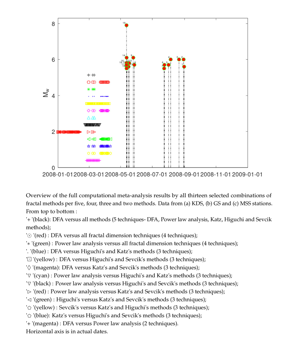
In Figure 12 for the KDS station, as with DFA and the fractal dimension calculation techniques, a first period is observed up to window 2200 (approximately 120) with scattered successive fractal windows with . These fractal epochs correspond to predictable Class-I segments with interchange between persistency and antipersistency. According to publications (e.g., [91]) this is a sign of precursory activity. Interestingly, this epoch is almost identical to those identified with DFA and the three fractal dimension techniques and this is very important. Figure 13 for the GS station shows a first period between window 1 and 40 ( 1 to 58) and window 50-90 ( 73 to 131). Both these periods have areas with (Class I, persistent) and can be considered as precursory of the great Wenchuan earthquake. The last period at the end of the analysed windows has and, as with DFA and fractal dimension techniques is on low predictability and , hence of low precursory value. This combined finding provides more evidence. In Figure 14 for the MSS station, there are two periods, between window 30 ( 43) and window 60 ( 87), and, between window 70 ( 102) and window 110 ( 160). Although these periods are anti-persistent they are within the middle part of predictable value range of the Class-I category. Since the periods match with those of the other techniques there is probability that they might be signs (pre and post) of the great Wenchuan earthquake. As with DFA and fractal dimension techniques, there is a great post seismic region within the same period as the one identified with DFA and fractal techniques. It is very important that the findings of the techniques match even for the two other stations the PZHS and SPS. Both showed no successive fractal window. This fact reinforces the findings of the DFA and Higuchi’s and Sevcik’s for the MSS station. Evaluating the results presented so-far, there is a period up to 133 (day of occurrence of the great Wenchuan earthquake) which is systematically identified in all fractal analysis results, that is from all methods, for the KDS, GS and MSS stations, whereas the PSZH and SPS stations do not show any noteworthy such period. These fractal epochs are discussed and considered as pre-seismic signatures of the great Wenchuan earthquake. The recognition of signs in the KDS, GS and MSS stations and the lack of systematic signs of the PSZH and SPS stations is attributed to the different geological paths in association to the theory of asperities and the selectivity effects in earthquake related research. It is also extensively discussed, that finding periods of over- or under- threshold fractal values is significant, but most significant is the synthetic finding of common over- or under- threshold areas with different techniques (meta-analysis, Section 3.8). When, and if, such common locations are discovered, the scientific arguments for the existence of a seismic warnings concealed in the time series increases, making the claims stronger. It is therefore very important to apply meta-analysis to the fractal results of KDS, GS and MSS stations so as to increase the presented evidence. Meta-analysis in the PSZH and SPS station’s results is unnecessary since the corresponding signs are not enough. On the other hand, a so great earthquake as the Wenchuan, is expected to be associated with other earthquakes. Moreover, other earthquakes of the overall area might also explain warnings and there is a possibility that the presumed post-seismic sings might be also be pre-seismic of other earthquakes of the area and this is the first time to mention such a view in this paper. Towards this, the earthquakes of 2008 with 5.5 were accessed from USGS for an area greater than the inserted one of Figure 1 [109]. The latter reference presents online the selected area together with data of 19 earthquakes and a map representing it in a terrain of China. For integrity the data of these 19 earthquakes are presented in Table 2, whereas Figure 17 presents the earthquakes in a Google Earth Map after creating the corresponding map kml file from USGS and importing it to Google Earth. In this way, Figure 17 presents the earthquakes alternatively in comparison to USGS map [109].
In the consensus expressed above the final step of the related analysis should include: (a) the above 19 earthquakes (Wenchuan included); (b) the fractal results and the discussion on threshold setting presented in Figure 2, Figure 3, Figure 4, Figure 5, Figure 6, Figure 7, Figure 8, Figure 9, Figure 10, Figure 11, Figure 12, Figure 13, Figure 14, Figure 15 and Figure 16; (c) the logic of connecting fractal methods expressed in Section 3.8. Towards this Figure 18 presents combined plots for each station. This multi figure conceals all the important findings. Similar representation has been adopted in other publications as well [1,27,29,65]. The subplots are mixed and have several symbols. For this reason it is crucial to delineate the significant information given:
- (a)
-
All over- or under-threshold results of all fractal methods (step 1, meta-analysis) for the KDS, MSS and GS stations. The threshold results of each station are combined per two, three, four and five methods (step 2, meta-analysis) (total 13 combinations) versus all 19 earthquakes of Table 2 and Figure 17.As mentioned in the previous paragraph, it is not only to identify footprints by one or more techniques (done already here as well) but more important is to link different techniques focusing on similar aspects of the problem in hand. To achieve this:
- (1)
- The exact over or under threshold dates were located computationally from the fractal outputs of each station (step-1, meta analysis). These dates are Year, Month, Day, Hour for the HSR station KDS and Year, Month, Day for MSS and GS stations. This is done through a serial search.
- (2)
- The common threshold dates from all different techniques were found through an incremental computational search. The outputs used are from all methods and with up to 13 different combination of these. All outputs were generated through special software and are stored in computer for use.
- (3)
- The earthquake data from USGS [109] were transformed to an adequate ASCII file for the generation of the final plot.
- (b)
- Wherever the symbols of different methods coincide in time, this means that the signs of seismicity is provided by more than one method. If all 13 methods coincide this means that the evidence is maximised. More techniques pointing to similar findings, more rigid the evidence is. The reader should stress that the coincidence is done on the step 1 results, that is on the fractal outputs.
In the above sense and starting from the combined findings of lesser importance, it can be observed from sub figure a of Figure 18 that there are several windows of the combination of DFA versus Higuchi’s and Sevcik’s methods (⊡,plot needs zoom to show the details) which are in the period of all 19 earthquakes. The fact that there are three techniques that show this behaviour, makes these fractal disturbances noteworthy. However, it is not possible to discriminate whether these disturbances are post seismic of the the great Wenchuan earthquake or pre-seismic of another one of the area and this is a limitation of the present methodology. On the other hand, observing carefully the data of Table 2, it is seen that earthquakes 13-18 are practically the seismic sequence of the Wenchuan earthquake since all occurred the same day as earthquake 19. Especially 16-18 happened at the same hour. Moreover earthquakes 11 and 12 are also within the post sequence of the Wenchuan earthquake because it occurred just one (11) and two (12) days after. Moreover all earthquakes from 8-19 occurred on the same month (April 2008). This peculiar facts complicate the issue of discriminating the above common 3-technique concurrent findings from characterising as post- or pre-sesmic. This is not the case for the three co-occurrences of the combinations of the fractal dimension methods (-yellow, namely Sevcik’s versus Katz’s and Higuchi’s methods (3 techniques), -blue, viz. Katz’s versus Higuchi’s and Sevcik’s methods (3 techniques) and green ⊲, namely Higuchi’s versus Katz’s and Sevcik’s methods (3 techniques)). These occurred prior to events 7,6 and 5 but could be prior to 4,3,2,1 as well (decreasing time distance between fractal disturbance and earthquake occurrence) (all these sub figures need zoom as well).
The most significant finding of this paper is left for its last part. It is clearly observed in all sub-figures that the vast majority of coincidences are prior to the great Wenchuan earthquake (19) and its synchronous post-earthquakes (10-19). This is the most important observation and the reader should stress on it. It is not only one method, but all 13 methods which coincide. Moreover during this preparation phase of the great Wenchuan earthquake, there are far more coincidences of even 3 or less techniques as well (such as red ⊳-sub figure b, namely power law analysis versus Katz’s and Sevcik’s methods (3 techniques) and yellow ⊡, that is DFA versus Higuchi’s and Sevcik’s methods (3 techniques)). In the most emphatic manner it is here declared that all these fractal disturbances (importantly, with results from meta-analysis), are, most possibly, due to the great Wenchuan earthquake. This is the most important finding of this paper and is left as last to place emphasis. It is the great magnitude of the Wenchuan, the post-seismic activity of it in association to the novel linking-combining several different fractal techniques that managed to outline such an important finding.
Conclusions
This study investigates the fractal patterns hidden in one-year radon in groundwater disturbances derived from five stations in China before and after the devastating Wenchuan (=7.9) shallow (depth=19 ) earthquake occurred on May 12, 2008 ( 133). The data is analysed with five distinct fractal techniques (DFA, fractal dimensions with Higuchi, Katz, and Sevcik methods and power-law analysis). Sliding windows of step 1 are utilised in segmented portions glided throughout each signal. Via literature-based thresholds, several notable areas are found in the fractal variations of the KDS, GS and MSS station data, while non-significant fractal portions are found in the signals of PZHS and SPS stations. Up to 133 (12 May 2008), several critical epochs are located in the signals of KDS, GS and MSS stations. In specific, the DFA exponents during these epochs are () whereas several exponents are above 1.8 (). The fractal dimension epochs exhibit Katz’s fractal dimensions around 1.0 and 1.2 (), Higuchi’s dimensions between 1.5 and 2 ()and Sevcik’s dimensions between 1 and 1.5 (). Several power-law b exponents are above 1.7 and numerous are above 2.0. All these are in agreement with precursory fractional Brownian motion signal parts. The differentiations of the KDS-GS-MSS stations versus the PZHS-SPS ones are attributed to the geological background with the theories of asperities (fractional Brownian motion profiles relative roughness) and selectivity. As a systematic last action, all results of the KDS-GS-MSS stations are analysed using a novel two-step, fully-computerized methodology which locates the exact out-of-threshold fractal areas and combines the outcomes of the different methods per five, four, three, and two (maximum 13 common combinations) in association with 19 earthquakes of .5.5 of the greater area. The vast majority of the different-technique combinations showed coincidences prior to the great Wenchuan earthquake and its synchronous post-earthquakes. This important finding is justified is not only with one method, but, in many cases, with all 13 different methods. Critical epochs after the Wenchuan earthquake are attributed to other earthquakes of the area whereas the post-seismic view can also be accepted. The combined results in association with the great earthquake’s magnitude and small depth make the findings of this paper promising for earthquake related studies.
Author Contributions
Conceptualization, Dimitrios Nikolopoulos; Data curation, Aftab Alam and Dimitrios Nikolopoulos; Formal analysis, Aftab Alam, Dimitrios Nikolopoulos, and Nanping Wang; Investigation, Aftab Alam, Dimitrios Nikolopoulos and Nanping Wang; Methodology, Aftab Alam and Dimitrios Nikolopoulos; Resources, Aftab Alam and Nanping Wang; Software, Dimitrios Nikolopoulos; Supervision, Dimitrios Nikolopoulos and Nanping Wang; Visualization, Aftab Alam and Dimitrios Nikolopoulos; Writing – original draft, Dimitrios Nikolopoulos; Writing – review & editing, Aftab Alam and Nanping Wang.
References
- Nikolopoulos, D.; Petraki, E.; Yannakopoulos, P.H.; Priniotakis, G.; Voyiatzis, I.; Cantzos, D. Long-lasting patterns in 3 kHz electromagnetic time series after the ML= 6.6 earthquake of 2018-10-25 near Zakynthos, Greece. Geosciences 2020, 10, 235. [Google Scholar] [CrossRef]
- Cicerone, R.; Ebel, J.; Britton, J. A systematic compilation of earthquake precursors. Tectonophysics 2009, 476, 371–396. [Google Scholar] [CrossRef]
- HOUGH, S. The Great Quake Debate: The Crusader, the Skeptic, and the Rise of Modern Seismology; University of Washington Press, 2020.
- Hayakawa, M.; Hobara, Y. Current status of seismo-electromagnetics for short-term earthquake prediction. Geomatics, Natural Hazards and Risk 2010, 1, 115–155. [Google Scholar] [CrossRef]
- Molchanov, O.A.; Hayakawa, M. Seismo-Electromagnetics and Related Phenomena: History and Latest Results; Number A8, TERRAPUB: Tokyo, 2008; p. 189. [Google Scholar]
- Ouzounov, D.; Pulinets, S.; Hattori, K.; Taylor, P. Pre-Earthquake Processes: A Multidisciplinary Approach to Earthquake Prediction Studies Posters; Wiley. John Wiley and Sons., 2018; p. 384.
- Petraki, E.; Nikolopoulos, D.; Nomicos, C.; Stonham, J.; Cantzos, D.; et al. Electromagnetic Pre-earthquake Precursors: Mechanisms, Data and Models-A Review. J. Earth Sci. Clim. Change 2015, 6, 1–11. [Google Scholar]
- Petraki, E.; Nikolopoulos, D.; Panagiotaras, D.; Cantzos, D.; Yannakopoulos, P.; et al. Radon-222: A Potential Short-Term Earthquake Precursor. J Earth Sci Clim Change 2015, 6, 1–11. [Google Scholar]
- Uyeda, S.; Nagao, T.; Kamogawa, M. Short-term earthquake prediction: Current status of seismo-electromagnetics. Tectonophysics 2009, 470, 205–213. [Google Scholar] [CrossRef]
- Conti, L.; Picozza, P.; Sotgiu, A. A Critical Review of Ground Based Observations of Earthquake Precursors. Frontiers in Earth Science 2021, 9. [Google Scholar] [CrossRef]
- Ghosh, D.; Deb, A.; Sengupta, R. Anomalous radon emission as precursor of earthquake. J. Appl. Geophys. 2009, 187, 245–258. [Google Scholar] [CrossRef]
- Liu, C.; Dong, P.; Zhu, B.; Shi, Y. Stress Shadow on the Southwest Portion of the Longmen Shan Fault Impacted the 2008 Wenchuan Earthquake Rupture. Journal of Geophysical Research: Solid Earth 2018, 123, 9963–9981. [Google Scholar] [CrossRef]
- Yin, Y.; Wang, F.; Sun, P. Landslide hazards triggered by the 2008 Wenchuan earthquake, Sichuan, China. Landslides 2009, 6, 139–152. [Google Scholar] [CrossRef]
- Xu, Y.; Koper, K.D.; Sufri, O.; Zhu, L.; Hutko, A.R. Rupture imaging of the Mw 7.9 12 May 2008 Wenchuan earthquake from back projection of teleseismic P waves. Geochemistry, Geophysics, Geosystems 2009, 10. [Google Scholar] [CrossRef]
- Nikolopoulos, D.; Matsoukas, C.; Yannakopoulos, P.H.; Petraki, E.; Cantzos, D.; Nomicos, C. Long-Memory and Fractal Trends in Variations of Environmental Radon in Soil: Results from Measurements in Lesvos Island in Greece, J Earth Sci. J. Earth Sci. Clim. Change 2018, 9, 1–11. [Google Scholar]
- Rafique, M.; Iqbal, J.; Shah, S.A.A.; Alam, A.; Lone, K.J.; Barkat, A.; Shah, M.A.; Qureshi, S.A.; Nikolopoulos, D. On fractal dimensions of soil radon gas time series. Journal of Atmospheric and Solar-Terrestrial Physics 2022, 227, 105775. [Google Scholar] [CrossRef]
- Shi, Z.; Wang, G.; Wang, C.y.; Manga, M.; Liu, C. Comparison of hydrological responses to the Wenchuan and Lushan earthquakes. Earth and Planetary Science Letters 2014, 391, 193–200. [Google Scholar] [CrossRef]
- Ren, H.; Liu, Y.; Yang, D. A preliminary study of post-seismic effects of radon following the Ms 8.0 Wenchuan earthquake. Radiation Measurements 2012, 47, 82–88. [Google Scholar] [CrossRef]
- Mandelbrot, B.B.; Ness, J.W.V. Fractional Brownian motions, fractional noises and applications. J. Soc. Ind. Appl. Math 1968, 10, 422–437. [Google Scholar] [CrossRef]
- Morales, I.O.; Landa, O.; Fossion, R.; Frank, A. Scale invariance, self-similarity and critical behaviour in classical and quantum system. J. Phys. Conf. Ser. 2012, 380. [Google Scholar] [CrossRef]
- Musa, M.; Ibrahim, K. Existence of long memory in ozone time series. Sains Malaysiana 2012, 41, 1367–1376. [Google Scholar]
- Vadrevu, K.P. Fractal analysis revealed persistent correlations in long-term vegetation fire data in most South and Southeast Asian countries. Environmental Research Communications 2023, 5. [Google Scholar] [CrossRef]
- May, R.M. Simple mathematical models with very complicated dynamics. Nature 1976, 261, 459–467. [Google Scholar] [CrossRef]
- Sugihara, G.; May, R. Nonlinear forecasting as a way of distinguishing chaos from measurement error in time series. Nature 1990, 344, 734–741. [Google Scholar] [CrossRef]
- Liu, C.; Liang, J.; Li, Y.; Shi, K. Fractal analysis of impact of PM2.5 on surface O3 sensitivity regime based on field observations. Science of The Total Environment 2023, 858, 160136. [Google Scholar] [CrossRef]
- Pastén, D.; Pavez-Orrego, C. Multifractal time evolution for intraplate earthquakes recorded in southern Norway during 1980–2021. Chaos, Solitons & Fractals 2023, 167, 113000. [Google Scholar] [CrossRef]
- Nikolopoulos, D.; Moustris, K.; Petraki, E.; Cantzos, D. Long-memory traces in PM _ 10 time series in Athens, Greece: investigation through DFA and R/S analysis. Meteorology and Atmospheric Physics 2021, 133, 261–279. [Google Scholar] [CrossRef]
- Chelidze, T.; Matcharashvili, T.; Mepharidze, E.; Dovgal, N. Complexity in Geophysical Time Series of Strain/Fracture at Laboratory and Large Dam Scales: Review. Entropy 2023, 25. [Google Scholar] [CrossRef]
- Nikolopoulos, D.; Moustris, K.; Petraki, E.; D., K.; Cantzos, D. Fractal and long-memory traces in PM10 time series in Athens, Greece. Environmnets 2019, 6, 1–19.
- Hurst, H. Long term storage capacity of reservoirs. Trans. Am. Soc. Civ. Eng. 1951, 116, 770–808. [Google Scholar] [CrossRef]
- Hurst, H.; Black, R.; Simaiki, Y. Long-term Storage: An Experimental Study; Constable: London, 1965. [Google Scholar]
- Lopez, T.; Martınez-Gonzalez, C.; Manjarrez, J.; Plascencia, N.; Balankin, A. Fractal Analysis of EEG Signals in the Brain of Epileptic Rats, with and without Biocompatible Implanted Neuroreservoirs. AMM 2009, 15, 127–136. [Google Scholar] [CrossRef]
- Eftaxias, K.; Balasis, G.; Contoyiannis, Y.; Papadimitriou, C.; Kalimeri, M. Unfolding the procedure of characterizing recorded ultra low frequency, kHZ and MHz electromagnetic anomalies prior to the L’Aquila earthquake as pre-seismic ones - Part 2. NHESS 2010, 10, 275–294. [Google Scholar] [CrossRef]
- Kilcik, A.; Anderson, C.; Rozelot, J.; Ye, H.; Sugihara, G.; Ozguc, A. Nonlinear Prediction of Solar Cycle 24. Astrophysics J. 2009, 693, 1173–1177. [Google Scholar] [CrossRef]
- Chattopadhyay, A.; Khondekar, M. An investigation of the relationship between the CME and the Geomagnetic Storm. Astronomy and Computing 2023, 43, 100695. [Google Scholar] [CrossRef]
- Granero, M.S.; Segovia, J.T.; Perez, J.G. Some comments on Hurst exponent and the long memory processes on capital Markets. Physica A 2008, 387, 5543–5551. [Google Scholar] [CrossRef]
- Musaev, A.; Makshanov, A.; Grigoriev, D. The Genesis of Uncertainty: Structural Analysis of Stochastic Chaos in Finance Markets. Complexity 2023, 2023, 1302220. [Google Scholar] [CrossRef]
- Pérez-Sienes, L.; Grande, M.; Losada, J.C.; Borondo, J. The Hurst Exponent as an Indicator to Anticipate Agricultural Commodity Prices. Entropy 2023, 25. [Google Scholar] [CrossRef] [PubMed]
- Vogl, M. Hurst exponent dynamics of S&P 500 returns: Implications for market efficiency, long memory, multifractality and financial crises predictability by application of a nonlinear dynamics analysis framework. Chaos, Solitons & Fractals 2023, 166, 112884. [Google Scholar] [CrossRef]
- Dattatreya, G. Hurst Parameter Estimation from Noisy Observations of Data Traffic Traces. 4th WSEAS international conference on electronics, control and signal processing, 2005; 193–198. [Google Scholar]
- Wang, F.; Wang, H.; Zhou, X.; Fu, R. A Driving Fatigue Feature Detection Method Based on Multifractal Theory. IEEE Sensors Journal 2022, 22, 19046–19059. [Google Scholar] [CrossRef]
- Zhou, H.; Chang, F. The long-memory temporal dependence of traffic crash fatality for different types of road users. Physica A: Statistical Mechanics and its Applications 2022, 607, 128210. [Google Scholar] [CrossRef]
- Li, X.; Polygiannakis, J.; Kapiris, P.; Peratzakis, A.; Eftaxias, K.; Yao, X. Fractal spectral analysis of pre-epileptic seizures in terms of criticality. J. Neural Eng. 2005, 2, 11–16. [Google Scholar] [CrossRef]
- Escobar-Ipuz, F.; Torres, A.; García-Jiménez, M.; Basar, C.; Cascón, J.; Mateo, J. Prediction of patients with idiopathic generalized epilepsy from healthy controls using machine learning from scalp EEG recordings. Brain Research 2023, 1798, 148131. [Google Scholar] [CrossRef]
- Wijayanto, I.; Humairani, A.; Hadiyoso, S.; Rizal, A.; Prasanna, D.L.; Tripathi, S.L. Epileptic seizure detection on a compressed EEG signal using energy measurement. Biomedical Signal Processing and Control 2023, 85, 104872. [Google Scholar] [CrossRef]
- Rehman, S.; Siddiqi, A. Wavelet based Hurst exponent and fractal dimensional analysis of Saudi climatic dynamics. Chaos Solitons Fractals 2009, 39, 1081–1090. [Google Scholar] [CrossRef]
- Petraki, E. Electromagnetic Radiation and Radon-222 Gas Emissions as Precursors of Seismic Activity. PhD thesis, Department of Electronic and Computer Engineering, Brunel University London, UK, 2016.
- Fujinawa, Y.; Takahashi, K. Electromagnetic radiations associated with major earthquakes. Phys. Earth Planet Inter 1998, 105, 249–259. [Google Scholar] [CrossRef]
- Hayakawa, M.; Ida, Y.; Gotoh, K. Multifractal analysis for the ULF geomagnetic data during the Guam earthquake. In Electromagnetic Compatibility and Electromagnetic Ecology. In Proceedings of the IEEE 6th International Symposium on June 2005. 239-243; 2005; pp. 21–24. [Google Scholar]
- Hayakawa, M. VLF/LF radio sounding of ionospheric perturbations associated with earthquakes. Sensors 2007, 7, 1141–1158. [Google Scholar] [CrossRef]
- Nikolopoulos, D.; Alam, A.; Petraki, E.; Papoutsidakis, M.; Yannakopoulos, P.; Moustris, K.P. Stochastic and self-organisation patterns in a 17-year PM10 time series in Athens, Greece. Entropy 2021, 23, 307. [Google Scholar] [CrossRef] [PubMed]
- Skordas, E.S. On the increase of the "non-uniform" scaling of the magnetic field variations before the M(w)9.0 earthquake in Japan in 2011. Chaos 2014, 24, 023131. [Google Scholar] [CrossRef]
- Stanley, H.E. Powerlaws and universality. Nature 1995, 378, 597–600. [Google Scholar] [CrossRef]
- Sarlis, N.; Skordas, E.; Varotsos, P.; Nagao, T.; M. Kamogawa, M.; Tanaka, H.; Uyeda, S. Minimum of the order parameter fluctuations of seismicity before major earthquakes in Japan. In Proceedings of the Proc. Natl. Acad. Sci. USA, 2013, Vol. 110, 34, pp. 13734–13738.
- Becker, M.; Karpytchev, M.; Hu, A. Increased exposure of coastal cities to sea-level rise due to internal climate variability. Nature Climate Change, 2023; 1–8. [Google Scholar] [CrossRef]
- Ivanova, K.; Ausloos, M. Application of the detrended fluctuation analysis (DFA) method for describing cloud breaking. Physica A 1999, 274, 349–354. [Google Scholar] [CrossRef]
- Koscielny-Bunde, E.; Bunde, A.; Havlin, S.; Roman, H.E.; Goldreich, Y.; Schellnhuberet, H. Indication of a Universal Persistence Law Governing Atmospheric Variability. Phys. Rev. Lett. 1998, 81, 729–732. [Google Scholar] [CrossRef]
- Rahmani, F.; Fattahi, M.H. Climate change-induced influences on the nonlinear dynamic patterns of precipitation and temperatures (case study: Central England). Theoretical and Applied Climatology, 2023; 1–12. [Google Scholar] [CrossRef]
- Linhares, R.R. Fractional poisson process: Long-range dependence in DNA sequences. Model Assisted Statistics and Applications 2023, 18, 33–43. [Google Scholar] [CrossRef]
- Peng, C.; Mietus, J.; Havlin, S.; Stanley, H.; Goldberger, A. Long-range anti-correlations and non-Gaussian behavior of the heartbeat. Phys. Rev. Lett. 1993, 70, 1343–1346. [Google Scholar] [CrossRef]
- Buldyrev, S.V.; Goldberger, A.L.; Havlin, S.; Mantegna, R.N.; Matsa, M.E.; Peng, C.K.; Simons, M.; Stanley, H.E. Long-range correlation properties of coding and noncoding DNA sequences: GenBank analysis. Phys. Rev. E Stat. Phys. Plasmas Fluids Relat. Interdiscip. Topics 1995, 51, 5084–5091. [Google Scholar] [CrossRef]
- Ivanov, P.C.; Rosenblum, M.G.; Peng, C.K.; Mietus, J.E.; Havlin, S.; Stanley, H.E.; Goldberger, A.L. Multifractality in human heartbeat dynamics. Nature 1999, 399, 461–465. [Google Scholar] [CrossRef]
- Mateo-March, M.; Moya-Ramón, M.; Javaloyes, A.; Sánchez-Muñoz, C.; Clemente-Suárez, V.J. Validity of detrended fluctuation analysis of heart rate variability to determine intensity thresholds in elite cyclists. European Journal of Sport Science 2023, 23, 580–587. [Google Scholar] [CrossRef]
- Rogers, B.; Schaffarczyk, M.; Gronwald, T. Improved Estimation of Exercise Intensity Thresholds by Combining Dual Non-Invasive Biomarker Concepts: Correlation Properties of Heart Rate Variability and Respiratory Frequency. Sensors 2023, 23. [Google Scholar] [CrossRef] [PubMed]
- Alam, A.; Wang, N.; Zhao, G.; Mehmood, T.; Nikolopoulos, D. Long-lasting patterns of radon in groundwater at Panzhihua, China: Results from DFA, fractal dimensions and residual radon concentration. GEOCHEMICAL JOURNAL 2019, 53, 341–358. [Google Scholar] [CrossRef]
- Alam, A.; Wang, N.; Zhao, G.; Barkat, A. Implication of radon monitoring for earthquake surveillance using statistical techniques: a case study of Wenchuan earthquake. Geofluids 2020, 2020, 1–14. [Google Scholar] [CrossRef]
- Eftaxias, K.; Balasis, G.; Contoyiannis, Y.; Papadimitriou, C.; Kalimeri, M.; Athanasopoulou, L.; Nikolopoulos, S.; Kopanas, J.; Antonopoulos, G.; Nomicos, C. Unfolding the procedure of characterizing recorded ultra low frequency, kHZ and MHz electromagnetic anomalies prior to the L’Aquila earthquake as pre-seismic ones-Part 1. Nat. Hazard Earth Sys. 2009, 9, 1953–1971. [Google Scholar] [CrossRef]
- Gotoh, K.; Hayakawa, M.; Smirnova, N.; Hattori, K. Fractal analysis of seismogenic ULF emissions. Phys. Chem. Earth 2004, 29, 419–424. [Google Scholar] [CrossRef]
- Hayakawa, M.; Ida, Y.; Gotoh, K. Fractal (mono- and multi-) analysis for the ULF data during the 1993 Guam earthquake for the study of prefracture criticality. Current Development in Theory and Applications of Wavelets 2008, 2, 159–174. [Google Scholar]
- Varotsos, P.; Sarlis, N.; Skordas, E. Natural Time Analysis: The new view of time. Precursory Seismic Electric Signals, Earthquakes and other Complex Time- Series; Springer-Verlag: Berlin Heidelberg, 2011. [Google Scholar]
- Varotsos, P.A.; Sarlis, N.V.; Skordas, E.S. Order Parameter and Entropy of Seismicity in Natural Time before Major Earthquakes: Recent Results. Geosciences 2022, 12. [Google Scholar] [CrossRef]
- Hu, K.; Ivanov, P.; Chen, Z.; Carpena, P.; Stanley, H. Effect of trends on Detrended Fluctuation Analysis. Phys Rev E 2001, 64, 1–19. [Google Scholar] [CrossRef]
- Peng, C.; Buldyrev, S.; Simons, M.; Havlin, S.; Stanley, H.; Goldberger, A. On the mosaic organization of DNA sequences. Phys. Rev. E 1994, 49, 1685–1689. [Google Scholar] [CrossRef]
- Peng, C.; Havlin, S.; Stanley, H.; Goldberger, A. Quantification of scaling exponents and crossover phenomena in nonstationary heartbeat time series. Chaos 1995, 5, 82–87. [Google Scholar] [CrossRef] [PubMed]
- Peng, C.; Hausdor, J.; Havlin, S.; Mietus, J.; Stanley, H.; Goldberger, A. Multiple-time scales analysis of physiological time series under neural control. Physica A 1998, 249, 491–500. [Google Scholar] [CrossRef] [PubMed]
- Nikolopoulos, D.; Yannakopoulos, P.H.; Petraki, E.; Cantzos, D.; Nomicos, C. Long-Memory and Fractal Traces in kHz-MHz Electromagnetic Time Series Prior to the ML=6.1, 12/6/2007 Lesvos, Greece Earthquake: Investigation through DFA and Time-Evolving Spectral Fractals. J. Earth Sci. Clim. Change 2018, 9, 1–15. [Google Scholar]
- Nikolopoulos, D.; Petraki, E.; Nomicos, C.; Koulouras, G.; Kottou, S.; Yannakopoulos, P.H. Long-Memory Trends in Disturbances of Radon in Soil Prior ML=5.1 Earthquakes of 17 November 2014 Greece. J. Earth Sci. Clim. Change 2015, 6, 1–11. [Google Scholar]
- Katz, M. Fractals and the analysis of waveforms. Comput. Biol. Med. 1988, 18, 145–156. [Google Scholar] [CrossRef] [PubMed]
- Raghavendra, B.; Dutt, D.N. Computing Fractal Dimension of Signals using Multiresolution Box-counting Method. International Journal of Electrical, Computer, Energetic, Electronic and Communication Engineering 2010, 4, 183–198. [Google Scholar]
- Higuchi, T. Approach to an irregular time series on basis of the fractal theory. Physica D 1988, 31, 277–283. [Google Scholar] [CrossRef]
- de la Torre, F.C.; Ramirez-Rojas, A.; Pavia-Miller, C.; Angulo-Brown, F.; E, E.Y.; Peralta, J. A comparison between spectral and fractal methods in electrotelluric time series. Revista Mexicana de Fisica 1999, 45, 298–302. [Google Scholar]
- de la Torre, F.C.; Gonzaalez-Trejo, J.; Real-Ramírez, C.; Hoyos-Reyes, L. Fractal dimension algorithms and their application to time series associated with natural phenomena. J. Phys. Conf. Ser. 2013, 475, 1–10. [Google Scholar] [CrossRef]
- Sevcik, C. On fractal dimension of waveforms. Chaos Solit. Fract. 2006, 27, 579–580. [Google Scholar] [CrossRef]
- Cantzos, D.; Nikolopoulos, D.; Petraki, E.; Yannakopoulos, P.H.; Nomicos, C. Earthquake precursory signatures in electromagnetic radiation measurements in terms of day-to-day fractal spectral exponent variation: analysis of the eastern Aegean 13/04/2017–20/07/2017 seismic activity. J. Seismol. 2018, 22, 1499–1513. [Google Scholar] [CrossRef]
- Ida, Y., H.; M. . Fractal analysis for the ULF data during the 1993 Guam earthquake to study prefracture criticality. Nonlin. Processes Geophys. 2012, 13, 409–412. [Google Scholar] [CrossRef]
- Ida, Y., Y.; Li, D.; Q. , S.; H., H.; M.. Fractal analysis of ULF electromagnetic emissions in possible association with earthquakes in China. Nonlin. Processes Geophys. 2012, 19, 577–583. [Google Scholar] [CrossRef]
- Smirnova, N.; Hayakawa, M. Fractal characteristics of the ground-observed ULF emissions in relation to geomagnetic and seismic activities. J. Atmos. Sol. Ter. Phy. 2007, 69, 1833–1841. [Google Scholar] [CrossRef]
- Yonaiguchi, N.; Ida, Y.; Hayakawa, M.; Masuda, S. Fractal analysis for VHF electromagnetic noises and the identification of preseismic signature of an earthquake. J. Atmos. Sol. Ter. Phy. 2007, 69, 1825–1832. [Google Scholar] [CrossRef]
- Eftaxias, K. Footprints of non-extensive Tsallis statistics, self-affinity and universality in the preparation of the L’Aquila earthquake hidden in a pre-seismic EM emission. Physica A 2010, 389, 133–140. [Google Scholar] [CrossRef]
- Kapiris, P.; Peratzakis, J.P.A.; Nomikos, K.; K. Eftaxias. VHF-electromagnetic evidence of the underlying pre-seismic critical stage. Earth Planets Space 2002, 54, 1237–1246. [Google Scholar] [CrossRef]
- Nikolopoulos, D.; Petraki, E.; Marousaki, A.; Potirakis, S.; Koulouras, G.; Nomicos, C.; Panagiotaras, D.; Stonhamb, J.; Louizi, A. Environmental monitoring of radon in soil during a very seismically active period occurred in South West Greece. J. Environ. Monit. 2012, 14, 564–578. [Google Scholar] [CrossRef]
- Alam, A.; Wang, N.; Petraki, E.; Barkat, A.; Huang, F.; Shah, M.A.; Cantzos, D.; Priniotakis, G.; Yannakopoulos, P.H.; Papoutsidakis, M.; et al. Fluctuation Dynamics of Radon in Groundwater Prior to the Gansu Earthquake, China (22 July 2013: M s= 6.6): Investigation with DFA and MFDFA Methods. Pure and Applied Geophysics 2021, 178, 3375–3395. [Google Scholar] [CrossRef]
- Telesca, L.; Lasaponara, R. Vegetational patterns in burned and unburned areas investigated by using the detrended fluctuation analysis. Physica A 2006, 368, 531–535. [Google Scholar] [CrossRef]
- Eftaxias, K.; Contoyiannis, Y.; Balasis, G.; Karamanos, K.; Kopanas, J.; Antonopoulos, G.; Koulouras, G.; Nomicos, C. Evidence of fractional-Brownian-motion-type asperity model for earthquake generation in candidate pre-seismic electromagnetic emissions. Nat. Hazard Earth Sys. 2008, 8, 657–669. [Google Scholar] [CrossRef]
- Varotsos, P.; Alexopoulos, K. Physical properties of the variations of the electric field of the earth preceding earthquakes, I. Tectonophysics 1984, 110, 73–98. [Google Scholar] [CrossRef]
- Varotsos, P.; Alexopoulos, K. Physical properties of the variations of the electric field of the earth preceding earthquakes, II. Tectonophysics 1984, 110, 99–125. [Google Scholar] [CrossRef]
- Varotsos, P.; Sarlis, N.; Lazaridou, M.B.N. Statistical evaluation of earthquake prediction results. Comments on the success rate and alarm rate, Acta Geophys. Pol 1996, 44, 329–347. [Google Scholar]
- Varotsos, P.; Sarlis, N.; Skordas, E. Magnetic field variations associated with SES. The instrumentation used for investigating their detectability. Proc Jpn Acad Ser B 2001, 77, 87–92. [Google Scholar] [CrossRef]
- Petraki, E.; Nikolopoulos, D.; Chaldeos, Y.; Koulouras, G.; Nomicos, C.; Yannakopoulos, P.H.; Kottou, S.; Stonham, J. Fractal evolution of MHz electromagnetic signals prior to earthquakes: results collected in Greece during 2009. Geomatics, Natural Hazards and Risk 2016, 7, 550–564. [Google Scholar] [CrossRef]
- Pinault, J.; Baubron, J. Signal processing of soil gas radon, atmospheric pressure, moisture, and soil temperature data: A new approach for radon concentration modeling. J. Geoph. Res. Sol. EA 1996, 101, 3157–3171. [Google Scholar] [CrossRef]
- Eftaxias, K.; Panin, V.; Deryugin, Y. Evolution-EM signals before earthquakes in terms of mesomechanics and complexity. Phys. Chem. Earth 2007, 29, 445–451. [Google Scholar] [CrossRef]
- K. Eftaxias, V. Sgrigna, T.C. Mechanical and electromagnetic phenomena accompanying preseismic deformation: From laboratory to geophysical scale. Tectonophysics 2007, 341, 1–5. [Google Scholar]
- Gotoh, K.; Hayakawa, M.; Smirnova, N. Fractal analysis of the ULF geomagnetic data obtained at Izu Peninsula, Japan in relation to the nearby earthquake swarm of June-August 2000. Nat. Haz. Earth Sys. 2003, 3, 229–234. [Google Scholar] [CrossRef]
- Hayakawa, M.; Kawate, R.; Molchanov, O.; Yumoto, K. Results of ultra-low-frequency magnetic field measurements during the Guam earthquake of 8 August 1993. Geophys. Res. Lett. 1996, 23, 241–244. [Google Scholar] [CrossRef]
- Hayakawa, M.; Itoh, T.; Hattori, K.; Yumoto, K. ULF electromagnetic precursors for an earthquake at Biak, Indonesia on February 17, 1996. Geophys. Res. Lett. 2000, 27, 1531–1534. [Google Scholar] [CrossRef]
- Kapiris, P.; Eftaxias, K.; Nomikos, K.; Polygiannakis, J.; Dologlou, E.; Balasis, G.; Bogris, N.; Peratzakis, A.; Hadjicontis, V. Evolving towards a critical point: A possible electromagnetic way in which the critical regime is reached as the rupture approaches. Nonlinear Proc. Geoph. 2003, 10, 1–14. [Google Scholar] [CrossRef]
- Smirnova, N.; Hayakawa, M.; Gotoh, K. Precursory behavior of fractal characteristics of the ULF electromagnetic fields in seismic active zones before strong earthquakes. Phys. Chem. Earth 2004, 29, 445–451. [Google Scholar] [CrossRef]
- Smirnova, N.A.; Kiyashchenko, D.A.T.; N. , V.; Hayakawa, M. Multifractal Approach to Study the Earthquake Precursory Signatures Using the Ground-Based Observations. Review of Applied Physics 2013, 2, 3. [Google Scholar]
- USGS. Available online: https://earthquake.usgs.gov/earthquakes/map/?extent=22.41103,91.51611&extent=35.56798,113.57666&range=search&baseLayer=terrain&timeZone=utc&search=%7B%22name%22:%22Search%20Results%22,%22params%22:%7B%22starttime%22:%222008-01-01%2000:00:00%22,%22endtime%22:%222009-01-01%2000:00:00%22,%22maxlatitude%22:36.844,%22minlatitude%22:22.999,%22maxlongitude%22:116.323,%22minlongitude%22:96.504,%22minmagnitude%22:5.5,%22orderby%22:%22time%22%7D%7D (accessed on 26 May 2023).
Figure 1.
Location of the epicentre of the Wenchuan earthquake, showing the radon in groundwater monitoring stations together with elevation data and the significant geological faults. The location of the presented area within China is shown in the inserted sub-figure on the bottom right.The codes of stations are given in Table 1.
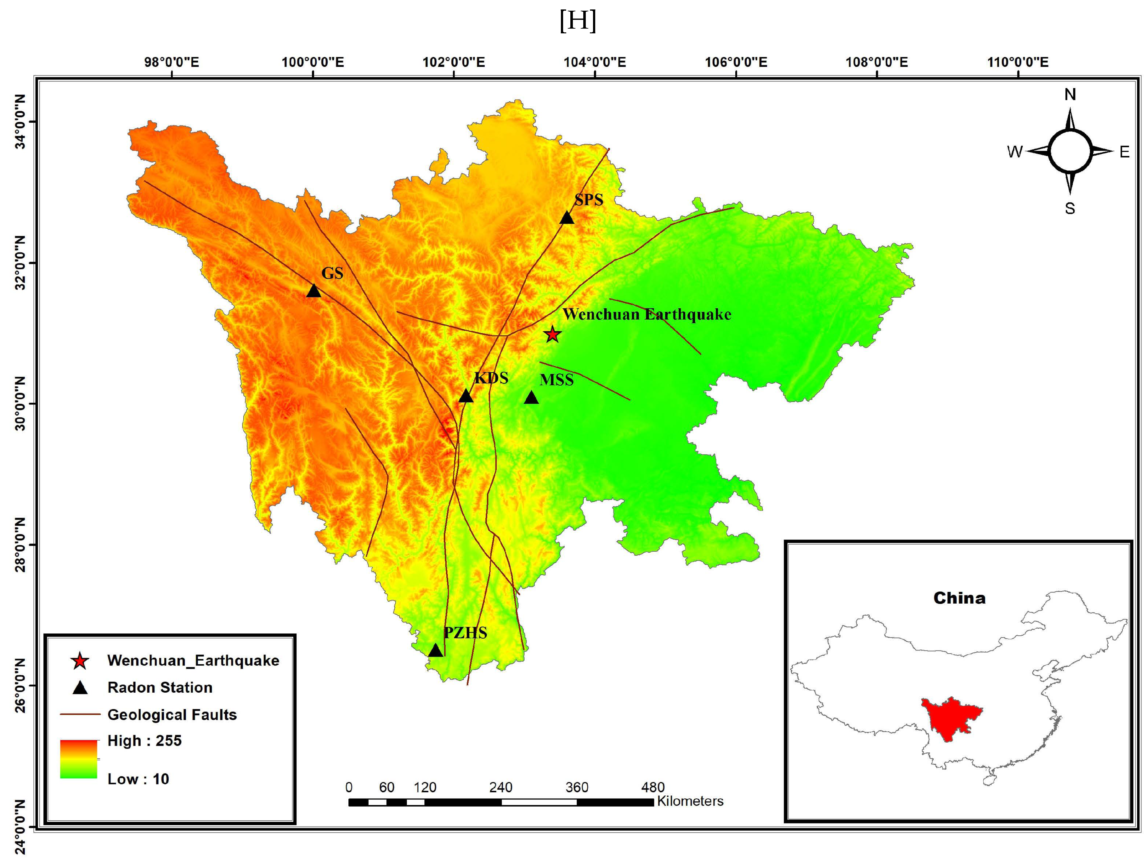
Figure 2.
Results of DFA. KDS station (ID=3).Window of 64 samples and step of 1 sample. From bottom to top: (a) Radon in groundwater time series; (b) The Spearman’s correlation coefficient of the goodness of the linear fit of versus n in every 64-sample window; (c) The scaling exponent (DFA slope). The horizontal axis is from the beginning (2018/1/1) to the end (2018/12/31) of measurements. The measurement sampling rate is 1 . For the window segmentation please see text.
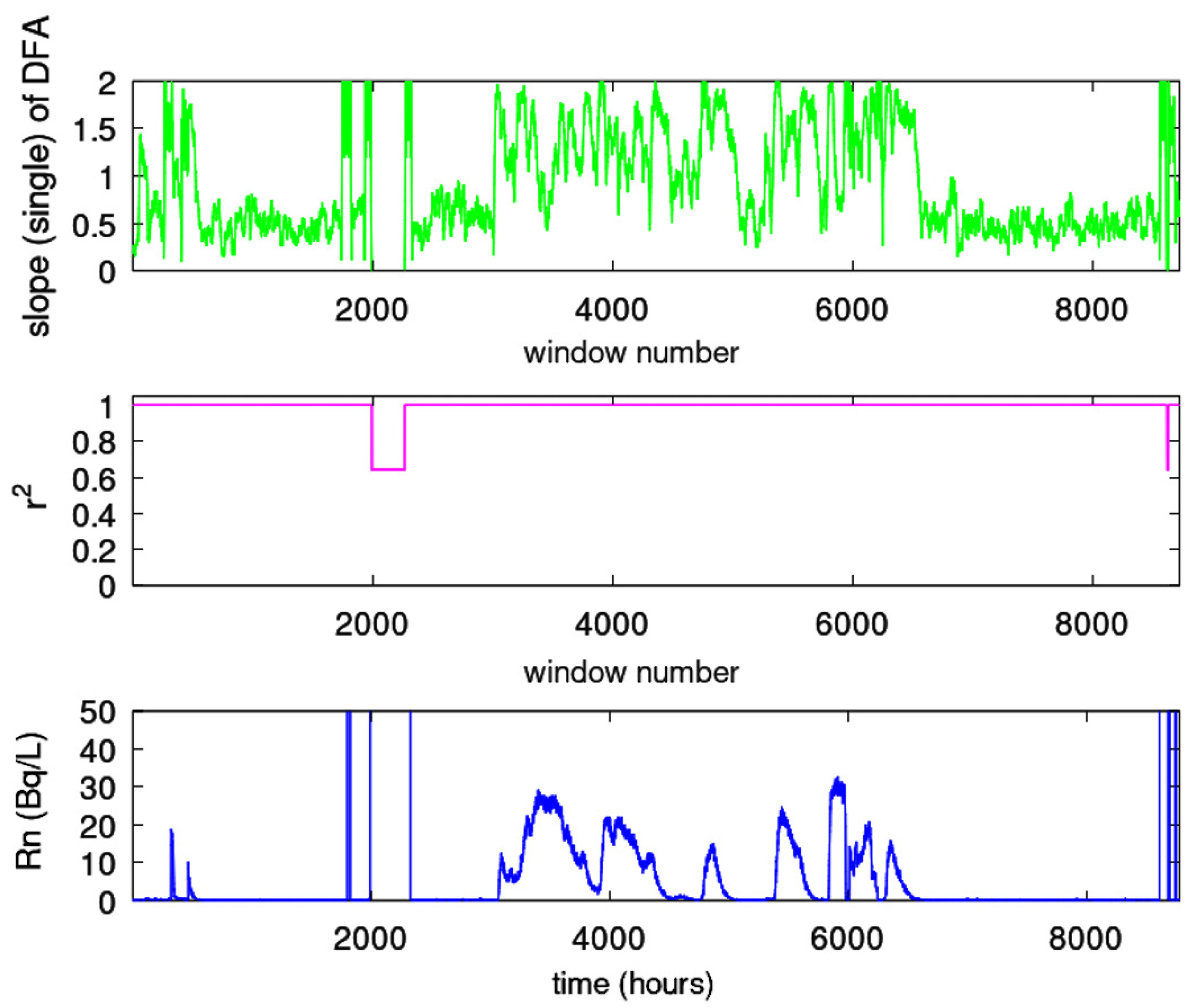
Figure 3.
Results of DFA. GS station (ID=82). Window of 64 samples and step of 1 sample. From bottom to top: (a) Radon in groundwater time series; (b) The Spearman’s correlation coefficient of the goodness of the linear fit of versus n in every 64-sample window; (c) The scaling exponent (DFA slope). The horizontal axis is from the beginning (2018/1/1) to the end (2018/12/31) of measurements. The measurement sampling rate is 1 . For the window segmentation please see text.
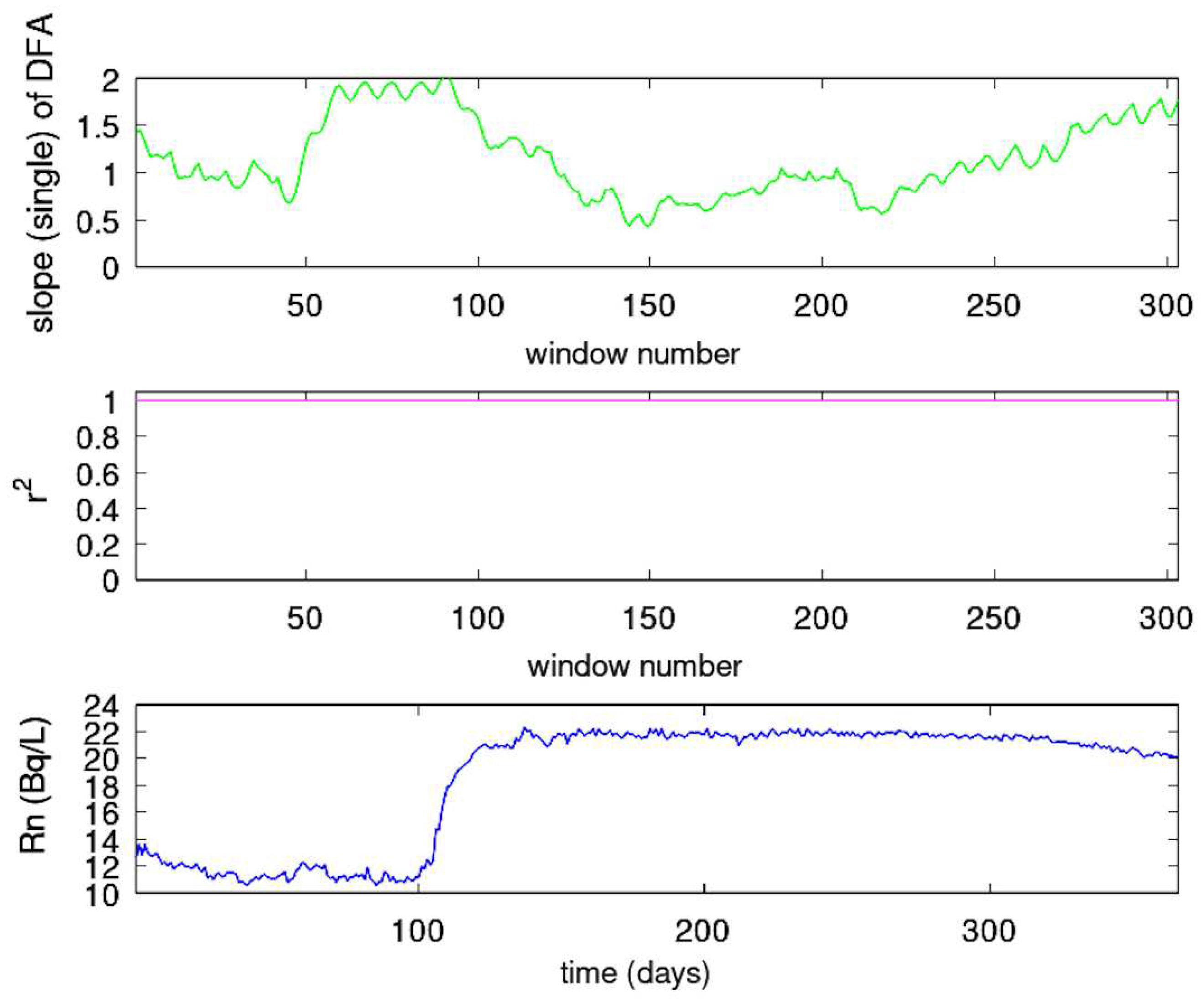
Figure 4.
Results of DFA. MSS station (ID=83). Window of 64 samples and step of 1 sample. From bottom to top: (a) Radon in groundwater time series; (b) The Spearman’s correlation coefficient of the goodness of the linear fit of versus n in every 64-sample window; (c) The scaling exponent (DFA slope). The horizontal axis is from the beginning (2018/1/1) to the end (2018/12/31) of measurements. The measurement sampling rate is 1 . For the window segmentation please see text.
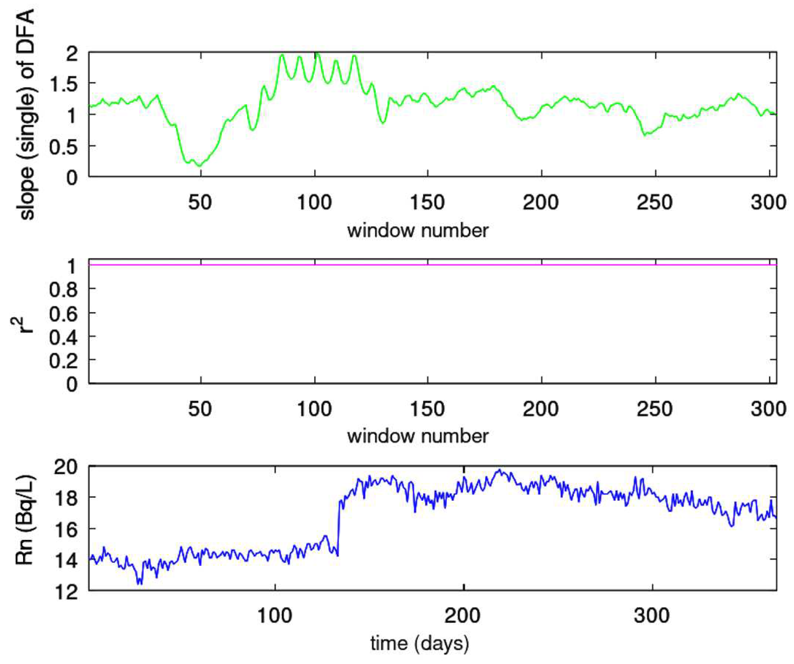
Figure 5.
Results of DFA. PZHS station (ID=143). Window of 64 samples and step of 1 sample. From bottom to top: (a) Radon in groundwater time series; (b) The Spearman’s correlation coefficient of the goodness of the linear fit of versus n in every 64-sample window; (c) The scaling exponent (DFA slope). The horizontal axis is from the beginning (2018/1/1) to the end (2018/12/31) of measurements. The measurement sampling rate is 1 . For the window segmentation please see text.

Figure 6.
Results of DFA. SPS station (ID=149). Window of 64 samples and step of 1 sample. From bottom to top: (a) Radon in groundwater time series; (b) The Spearman’s correlation coefficient of the goodness of the linear fit of versus n in every 64-sample window; (c) The scaling exponent (DFA slope). The horizontal axis is from the beginning (2018/1/1) to the end (2018/12/31) of measurements. The measurement sampling rate is 1 . For the window segmentation please see text.
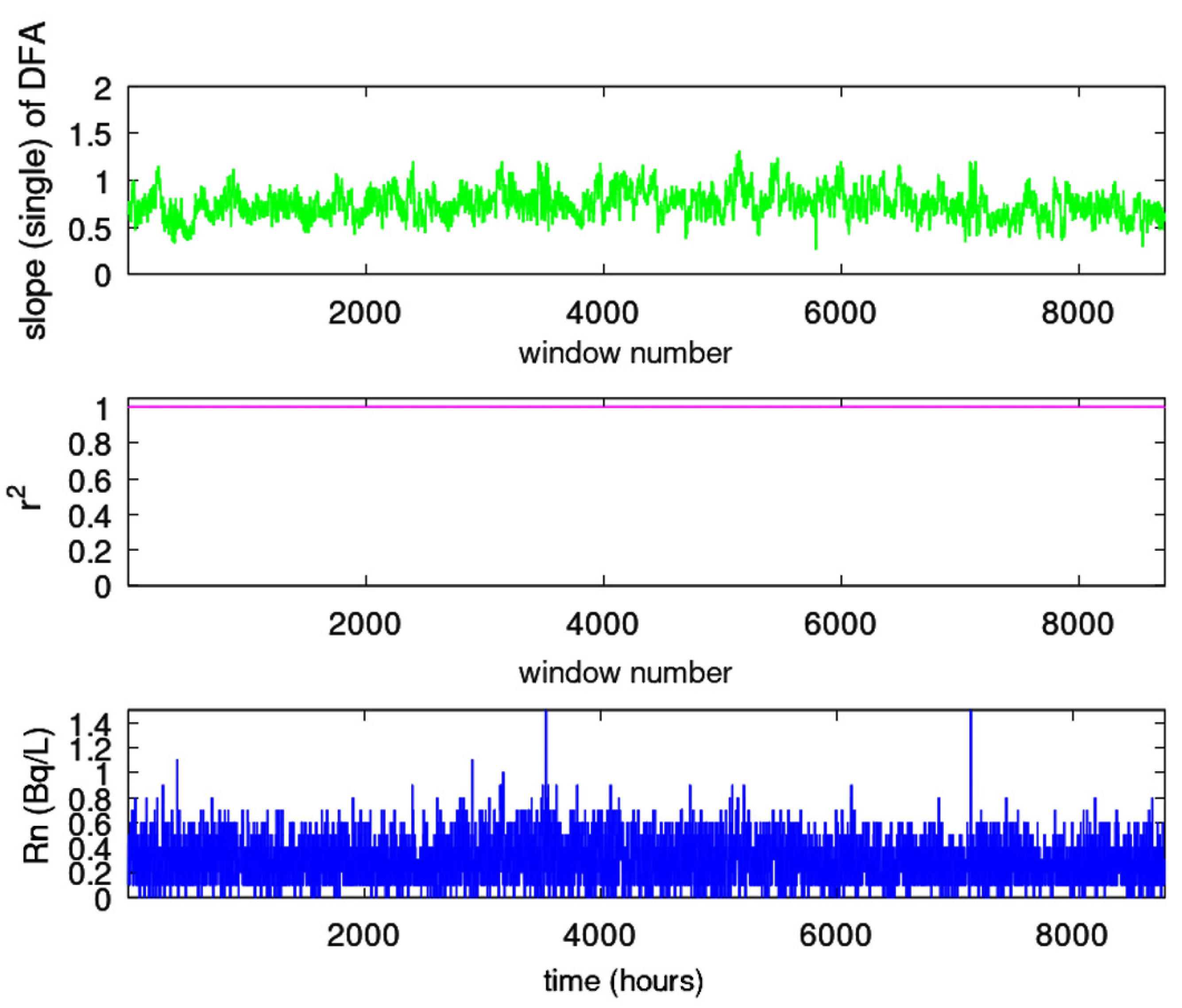
Figure 7.
Results from fractal dimension analysis. KDS station (ID=3). Window of 64 samples, 16 sub-categories of (Higuchi’s method and step of 1 sample. From bottom to top: (a) The radon in groundwater time-series and the fractal dimensions according to the algorithms of (b) Katz (KFD) ; (c) Higuchi (HFD) and (d) Sevcik (SFD). The horizontal axis is from the beginning (2018/1/1) to the end (2018/12/31) of measurements. The measurement sampling rate is 1 . For the window segmentation please see text.

Figure 8.
Results from fractal dimension analysis. GS station (ID=82). Window of 64 samples, 16 sub-categories of (Higuchi’s method and step of 1 sample. From bottom to top: (a) The radon in groundwater time-series and the fractal dimensions according to the algorithms of (b) Katz (KFD) ; (c) Higuchi (HFD) and (d) Sevcik (SFD). The horizontal axis is from the beginning (2018/1/1) to the end (2018/12/31) of measurements. The measurement sampling rate is 1 . For the window segmentation please see text.
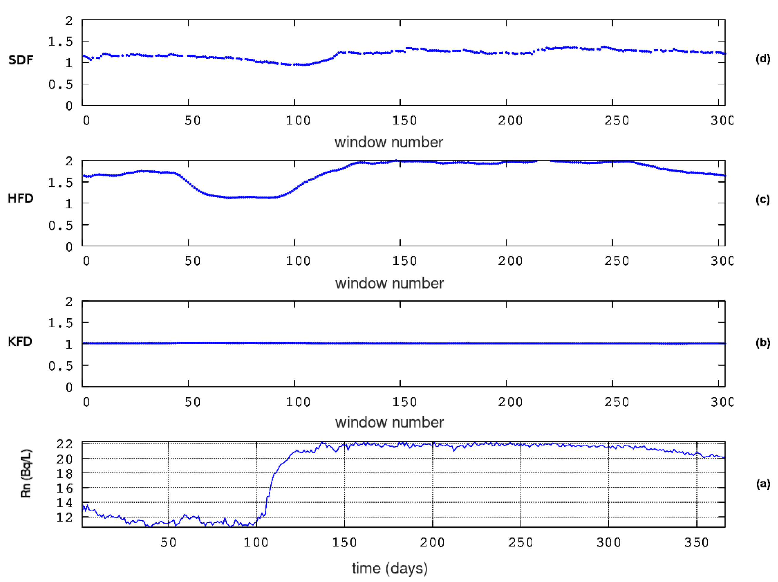
Figure 9.
Results from fractal dimension analysis. MSS station (ID=83). Window of 64 samples, 16 sub-categories of (Higuchi’s method and step of 1 sample. From bottom to top: (a) The radon in groundwater time-series and the fractal dimensions according to the algorithms of (b) Katz (KFD) ; (c) Higuchi (HFD) and (d) Sevcik (SFD). The horizontal axis is from the beginning (2018/1/1) to the end (2018/12/31) of measurements. The measurement sampling rate is 1 . For the window segmentation please see text.

Figure 10.
Results from fractal dimension analysis. PZHS station (ID=143). Window of 64 samples, 16 sub-categories of (Higuchi’s method and step of 1 sample. From bottom to top: (a) The radon in groundwater time-series and the fractal dimensions according to the algorithms of (b) Katz (KFD) ; (c) Higuchi (HFD) and (d) Sevcik (SFD). The horizontal axis is from the beginning (2018/1/1) to the end (2018/12/31) of measurements. The measurement sampling rate is 1 . For the window segmentation please see text.

Figure 11.
Results from fractal dimension analysis. SPS station (ID=149). Window of 64 samples, 16 sub-categories of (Higuchi’s method and step of 1 sample. From bottom to top: (a) The radon in groundwater time-series and the fractal dimensions according to the algorithms of (b) Katz (KFD) ; (c) Higuchi (HFD) and (d) Sevcik (SFD). The horizontal axis is from the beginning (2018/1/1) to the end (2018/12/31) of measurements. The measurement sampling rate is 1 . For the window segmentation please see text.
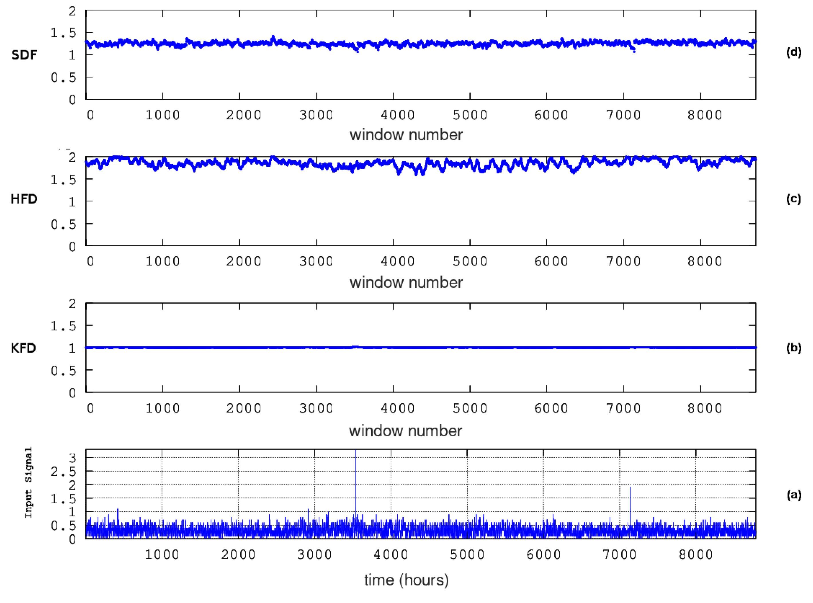
Figure 12.
Results from fractal analysis: KDS station (ID=3). Window of 128 samples and step of 1 sample. From bottom to top: (a) Radon in groundwater time-series; (b) Spearman’s correlation coefficient of the goodness of the linear fit of Equation (18); (c) Time evolution of power-law exponent. Blue areas represent the successive () fractal windows. Red areas are non-successive windows. The horizontal axis is from the beginning (2018/1/1) to the end (2018/12/31) of measurements. The measurement sampling rate is 1 . For the window segmentation please see text.
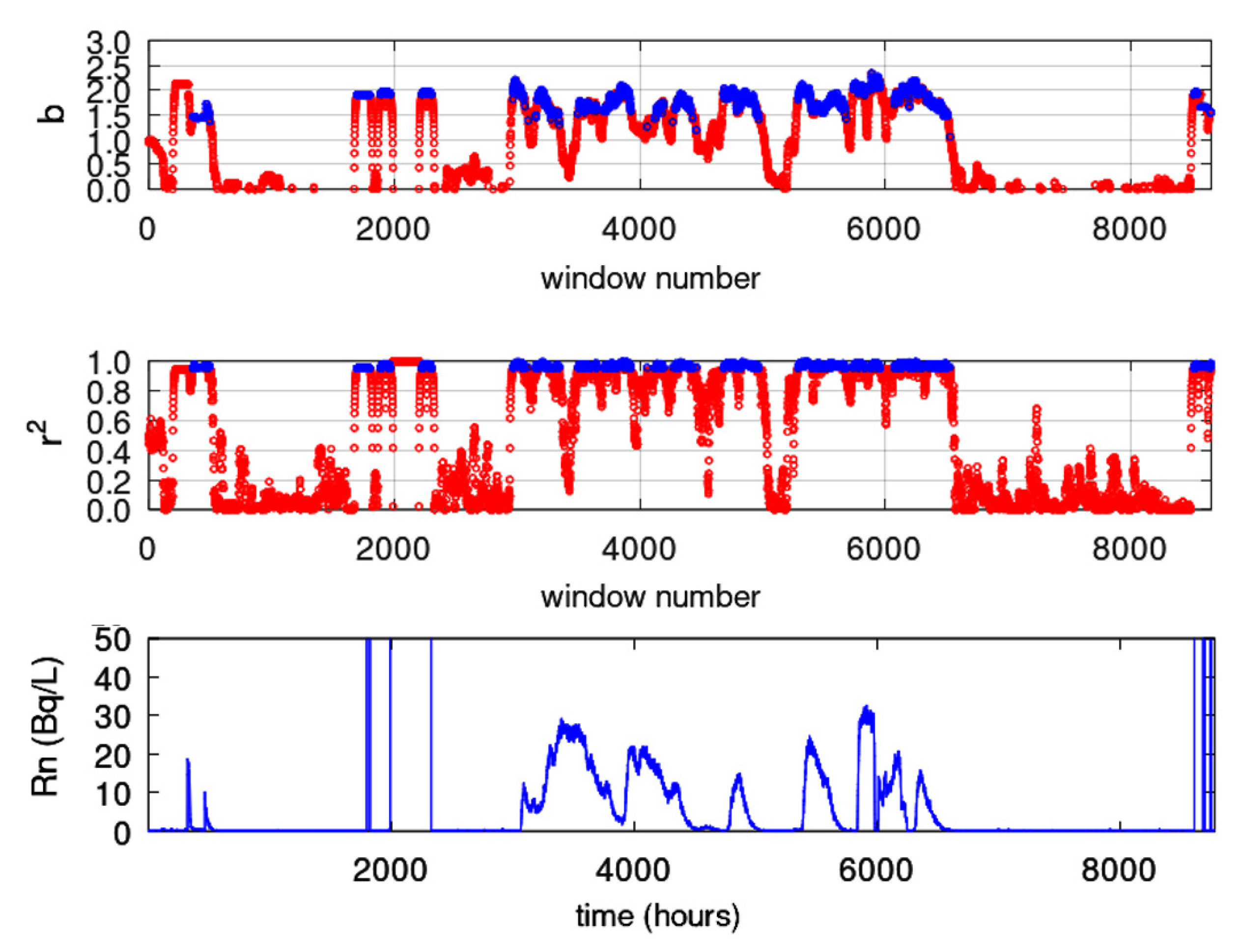
Figure 13.
Results from fractal analysis: GS station (ID=82). Window of 128 samples and step of 1 sample. From bottom to top: (a) Radon in groundwater time-series; (b) Spearman’s correlation coefficient of the goodness of the linear fit of Equation (18); (c) Time evolution of power-law exponent. Blue areas represent the successive () fractal windows. Red areas are non-successive windows. The horizontal axis is from the beginning (2018/1/1) to the end (2018/12/31) of measurements. The measurement sampling rate is 1 . For the window segmentation please see text.
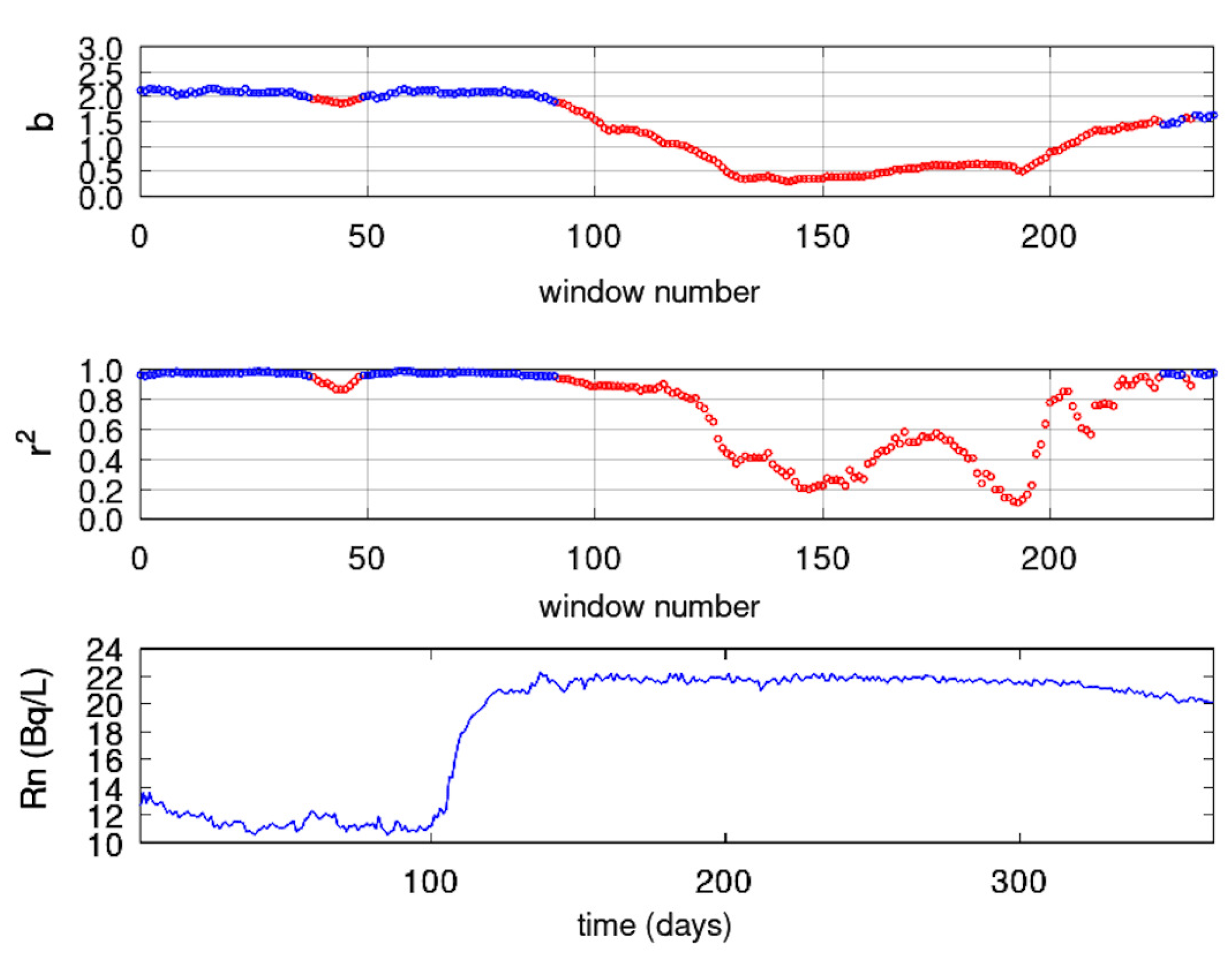
Figure 14.
Results from fractal analysis: MSS station (ID=83). Window of 128 samples and step of 1 sample. From bottom to top: (a) Radon in groundwater time-series; (b) Spearman’s correlation coefficient of the goodness of the linear fit of Equation (18); (c) Time evolution of power-law exponent. Blue areas represent the successive () fractal windows. Red areas are non-successive windows. The horizontal axis is from the beginning (2018/1/1) to the end (2018/12/31) of measurements. The measurement sampling rate is 1 . For the window segmentation please see text.
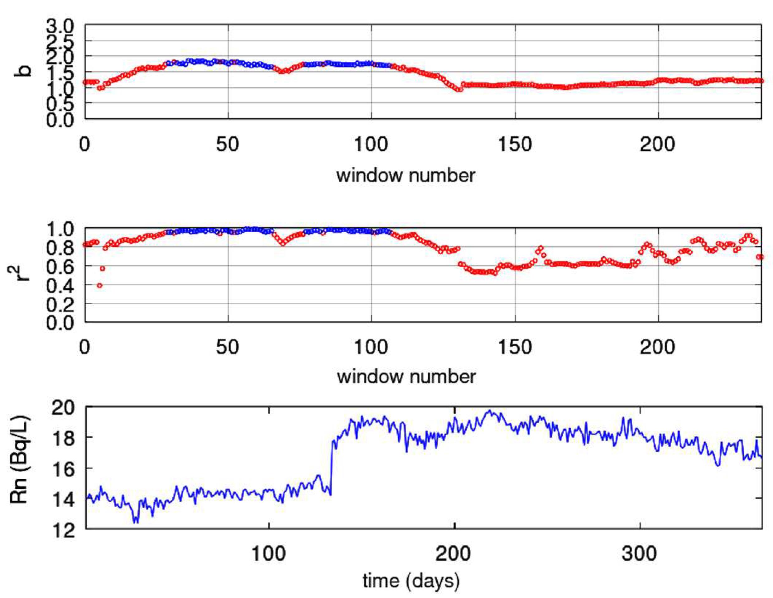
Figure 15.
Results from fractal analysis: PZHS station (ID=143). Window of 128 samples and step of 1 sample. From bottom to top: (a) Radon in groundwater time-series; (b) Spearman’s correlation coefficient of the goodness of the linear fit of Equation (18); (c) Time evolution of power-law exponent. Blue areas represent the successive () fractal windows. Red areas are non-successive windows. The horizontal axis is from the beginning (2018/1/1) to the end (2018/12/31) of measurements. The measurement sampling rate is 1 . For the window segmentation please see text.
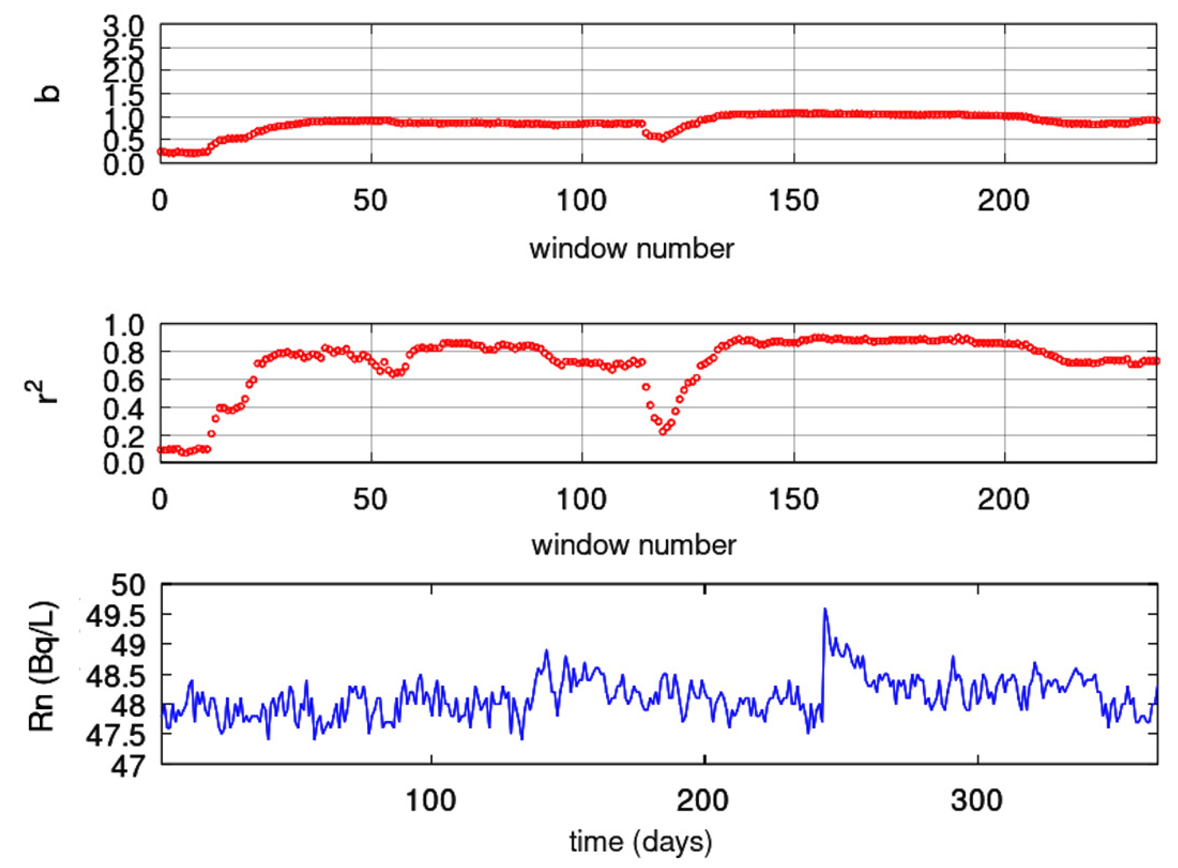
Figure 16.
Results from fractal analysis: SPS station (ID=149). Window of 128 samples and step of 1 sample. From bottom to top: (a) Radon in groundwater time-series; (b) Spearman’s correlation coefficient of the goodness of the linear fit of Equation (18); (c) Time evolution of power-law exponent. Blue areas represent the successive () fractal windows. Red areas are non-successive windows. The horizontal axis is from the beginning (2018/1/1) to the end (2018/12/31) of measurements. The measurement sampling rate is 1 . For the window segmentation please see text.
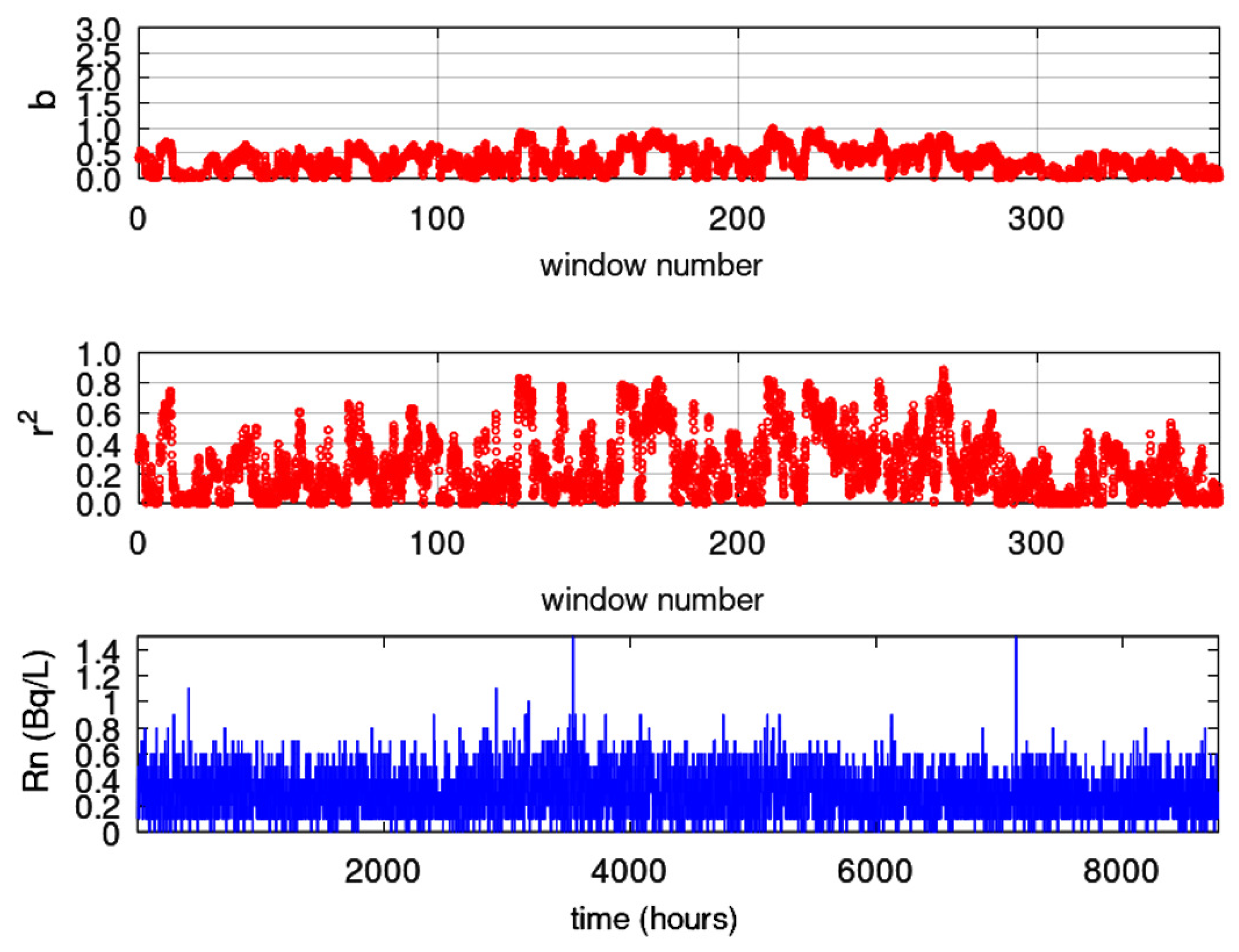
Figure 17.
Location of the earthquakes of 2008 with 5.5 for an area greater than the inserted one of Figure 1. The figure is created with Google Earth from the kml file from USGS. Greater circles are earthquakes with greater magnitude . The biggest circle near Sichuan is the great Wenchuan earthquake. The 19 presented earthquakes are shown in Table 2.
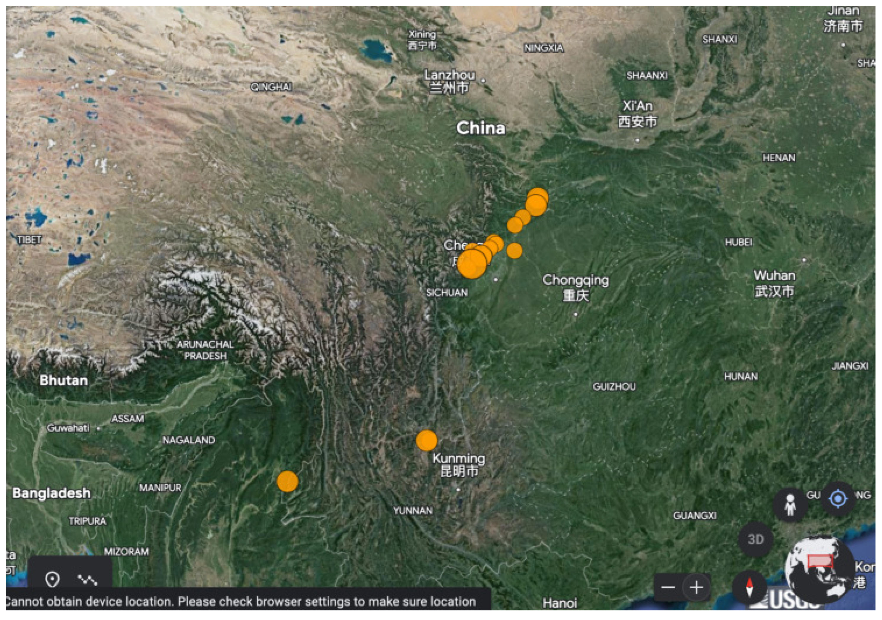
Figure 18.
Overview of the full computational meta-analysis results by all thirteen selected combinations of fractal methods per five, four, three and two methods. Data from (a) KDS, (b) GS and (c) MSS stations. From top to bottom: ’+ ’(black): DFA versus all methods (5 techniques- DFA, Power law analysis, Katz, Higuchi and Sevcik methods); ’⊙ ’(red) : DFA versus all fractal dimension techniques (4 techniques);’* ’(green): Power law analysis versus all fractal dimension techniques (4 techniques); ’. ’(blue) : DFA versus Higuchi’s and Katz’s methods (3 techniques); ’⊡ ’(yellow) : DFA versus Higuchi’s and Sevcik’s methods (3 techniques); ’◊ ’(magenta): DFA versus Katz’s and Sevcik’s methods (3 techniques); ’▿ ’(cyan) : Power law analysis versus Higuchi’s and Katz’s methods (3 techniques); ’▿ ’(black) : Power law analysis versus Higuchi’s and Sevcik’s methods (3 techniques); ’⊳ ’(red) : Power law analysis versus Katz’s and Sevcik’s methods (3 techniques); ’⊲ ’(green) : Higuchi’s versus Katz’s and Sevcik’s methods (3 techniques); ’ ⬠ ’(yellow) : Sevcik’s versus Katz’s and Higuchi’s methods (3 techniques); ’ ⬠ ’(blue): Katz’s versus Higuchi’s and Sevcik’s methods (3 techniques); ’+ ’(magenta) : DFA versus Power law analysis (2 techniques). Horizontal axis is in actual dates.
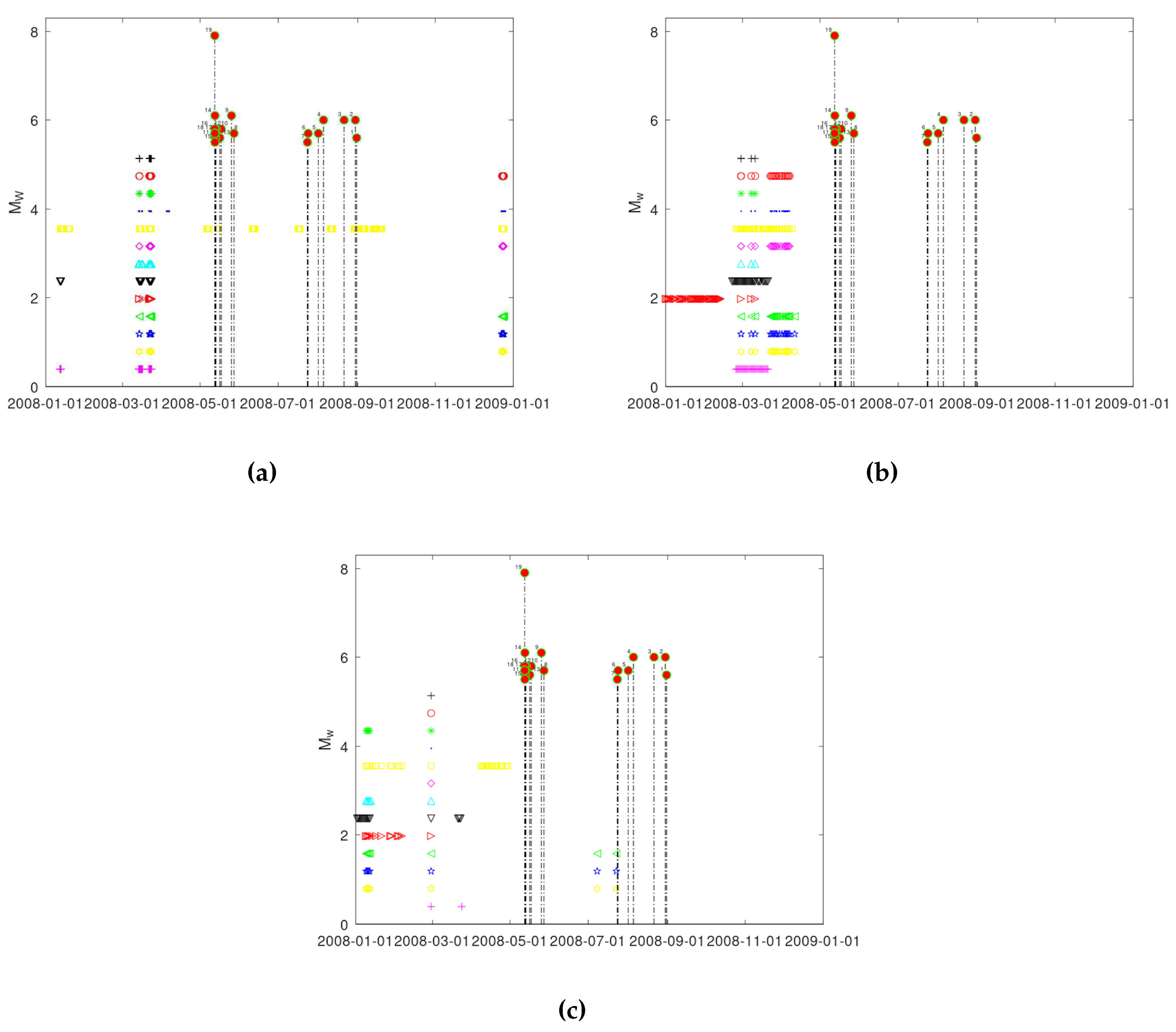

Table 1.
Radon in groundwater stations data. The numbers and coding of the stations are those globally adopted in China and the names refer to the actual locations. Distance is the distance from epicentre.
Table 1.
Radon in groundwater stations data. The numbers and coding of the stations are those globally adopted in China and the names refer to the actual locations. Distance is the distance from epicentre.
| Station Code | Station Name | Latitude | Longitude | Distance (Km) |
|---|---|---|---|---|
| KDS | Kangding station | 30.12 | 102.17 | 152.2 |
| GS | Ganzi station | 31.61 | 100.01 | 325.5 |
| MSS | Mingshan station | 30.1 | 103.1 | 105.6 |
| PZHS | Panzhihua station | 26.51 | 101.74 | 526.0 |
| SPS | Sonpan station | 32.65 | 103.6 | 182.5 |
Table 2.
Earthquakes of 2008 with 5.5 in China for the area presented in Figure 17. The last event (i/i 19) is the great Wenchuan earthquake
Table 2.
Earthquakes of 2008 with 5.5 in China for the area presented in Figure 17. The last event (i/i 19) is the great Wenchuan earthquake
| i/i | Year | Month | Day | Hour | Minute | Second | Latitude | Longitude | Depth (m) | |
|---|---|---|---|---|---|---|---|---|---|---|
| 1 | 2008 | 8 | 31 | 8 | 31 | 10 | 5.6 | 26.232 | 101.97 | 10 |
| 2 | 2008 | 8 | 30 | 8 | 30 | 53 | 6.0 | 26.241 | 101.889 | 11 |
| 3 | 2008 | 8 | 21 | 12 | 24 | 30 | 6.0 | 25.039 | 97.697 | 10 |
| 4 | 2008 | 8 | 5 | 9 | 49 | 17 | 6.0 | 32.756 | 105.494 | 6 |
| 5 | 2008 | 8 | 1 | 8 | 32 | 43 | 5.7 | 32.033 | 104.722 | 11 |
| 6 | 2008 | 7 | 24 | 9 | 30 | 9 | 5.7 | 32.747 | 105.542 | 10 |
| 7 | 2008 | 7 | 23 | 19 | 54 | 44 | 5.5 | 32.752 | 105.498 | 4 |
| 8 | 2008 | 5 | 27 | 8 | 37 | 51 | 5.7 | 32.71 | 105.54 | 10 |
| 9 | 2008 | 5 | 25 | 8 | 21 | 49 | 6.1 | 32.56 | 105.423 | 18 |
| 10 | 2008 | 5 | 17 | 8 | 25 | 48 | 5.8 | 32.24 | 104.982 | 9 |
| 11 | 2008 | 5 | 16 | 5 | 25 | 47 | 5.6 | 31.355 | 103.351 | 3 |
| 12 | 2008 | 5 | 13 | 7 | 7 | 8 | 5.8 | 30.89 | 103.194 | 9 |
| 13 | 2008 | 5 | 12 | 20 | 8 | 50 | 5.6 | 31.413 | 103.889 | 21.7 |
| 14 | 2008 | 5 | 12 | 11 | 11 | 2 | 6.1 | 31.214 | 103.618 | 10 |
| 15 | 2008 | 5 | 12 | 9 | 42 | 24 | 5.5 | 31.527 | 104.092 | 10 |
| 16 | 2008 | 5 | 12 | 6 | 43 | 14 | 5.8 | 31.211 | 103.715 | 10 |
| 17 | 2008 | 5 | 12 | 6 | 42 | 8 | 5.7 | 31.342 | 104.682 | 10 |
| 18 | 2008 | 5 | 12 | 6 | 61 | 56 | 5.7 | 31.586 | 104.032 | 10 |
| 19 | 2008 | 5 | 12 | 6 | 28 | 1 | 7.9 | 31.002 | 103.322 | 19 |
Disclaimer/Publisher’s Note: The statements, opinions and data contained in all publications are solely those of the individual author(s) and contributor(s) and not of MDPI and/or the editor(s). MDPI and/or the editor(s) disclaim responsibility for any injury to people or property resulting from any ideas, methods, instructions or products referred to in the content. |
© 2023 by the authors. Licensee MDPI, Basel, Switzerland. This article is an open access article distributed under the terms and conditions of the Creative Commons Attribution (CC BY) license (http://creativecommons.org/licenses/by/4.0/).
Copyright: This open access article is published under a Creative Commons CC BY 4.0 license, which permit the free download, distribution, and reuse, provided that the author and preprint are cited in any reuse.


