
Submitted:
19 June 2023
Posted:
20 June 2023
You are already at the latest version
Abstract
Decomposed fuzzy sets are the resent extension of intuitionistic fuzzy sets by incorporating functional and dysfunctional points of views to the definition of membership functions. This paper extends the Technique of Order Preference Similarity to the Ideal Solution (TOPSIS) method to the Decomposed Fuzzy TOPSIS (DF TOPSIS) method and applies it to a multi-criteria risk-based supplier selection problem under fuzziness. DF TOPSIS involves finding a positive ideal solution and a negative ideal solution and measuring the distance of each alternative to these solutions. The final ranking is obtained based on the proportion of distances to the positive and negative ideal solutions. The developed DF TOPSIS method incorporates the accuracy and consistency of expert judgments, enhancing the decision-making process. A sensitivity analysis is also presented in order to show the robustness of the obtained rankings by DF TOPSIS.
Keywords:
Intuitionistic fuzzy sets
; Decomposed fuzzy sets
; TOPSIS
; Risk analysis
; Supplier selection problem
1. Introduction
Intuitionistic fuzzy sets (IFS) were introduced by Atanassov [1] in order to include the hesitancy degrees of experts in their assessments. Since membership and non-membership degrees are complementary to one in ordinary fuzzy sets (OFS), it is assumed that an expert is not hesitant in assigning his/her judgments. The sum of the membership, non-membership, and hesitancy degrees are complementary to one in IFS, which makes IFS a superset of OFS. Two questions for each element in an IFS are enough to ask an expert to construct it. What is the membership degree of the considered element? And what is the non-membership degree of the considered element?
However, determining membership and non-membership degrees requires a deeper analysis since an assignment for membership or non-membership degrees may be a momentary erroneous assignment. To determine these degrees, more questions composed of functional and dysfunctional questions can be asked by an expert, making the set of two sub-IFS components. The total number of questions becomes four since two for membership and non-membership degrees of functional question and two for membership and non-membership degrees of dysfunctional question are asked by an expert. Such a fuzzy set can be represented by . Since the sum in each component, or is at most equal to one, the overall sum of two components can be at most equal to 2, providing that where : the membership degree of element x with functional point of view; : the non-membership degree of element x with functional point of view; : the membership degree of element x with dysfunctional point of view; : the non-membership degree of element x with dysfunctional point of view. This new extension type of IFS is called Decomposed Fuzzy Sets (DFS) [2]. The aim of DFS is to increase the accuracy and consistency of the judgments assigned by experts through functional and dysfunctional questions. Çebi et al. [2] used DFS in operational risk analysis in business processes in a more realistic and detailed way through functional and dysfunctional question-based membership functions. Cebi et al. [3] extended the analytic hierarchy process (AHP) method by using DFS making pairwise comparisons in AHP more reliable by considering the individual answers given by experts to the reciprocal questions under vagueness and impreciseness.
In this paper, Technique of Order Preference Similarity to the Ideal Solution whose acronym is TOPSIS is extended to decomposed fuzzy TOPSIS (DF TOPSIS) method and is applied to a multi-criteria supplier selection problem under fuzziness. As the name implies, the method is based on finding a positive ideal and a negative ideal solution and comparing the distance of each of the alternatives to these solutions. Then, based on a proportion of the distances of alternatives to the positive and negative ideal solutions, the final ranking is obtained. The developed DF TOPSIS has the ability of taking the accuracy and consistency of the assigned judgments by an expert into account.
The rest of this paper is organized as follows. Section 2 presents a literature review on intuitionistic fuzzy sets and their extensions. Section 3 presents the preliminaries of decomposed fuzzy sets. Section 4 includes the proposed DF TOPSIS method. Section 5 gives the application of the proposed DF TOPSIS method to a supplier selection problem. Section 6 concludes the paper.
2. Intuitionistic Fuzzy Sets and Their Extensions: Literature Review
Intuitionistic fuzzy sets (IFSs) were introduced by Atanassov in [1] as a generalization of ordinary fuzzy sets. In IFSs, the sum of degrees of membership and non-membership is not necessarily equal to one, letting another complementary parameter be incorporated to the membership function. This makes them more suitable for representing imprecise and vague information [4,5,6,7,8]. The degree of membership of an element in an IFS is defined as the degree to which the element belongs to a given set while the degree of non-membership represents the degree to which the element does not belong to the set without complementary feature requirement to one. Thus, the third parameter introduced in IFS is the degree of indeterminacy, which quantifies the degree of uncertainty associated with the membership and non-membership degrees.
IFS have been applied in a variety of fields including decision-making, pattern recognition, and image processing since IFS can handle situations where data are incomplete or uncertain, allowing for more robust decision-making even in situations where the available information is limited. The inclusion of a degree of non-membership and a complementary degree of indeterminacy makes IFS more adaptable to situations where the degree of uncertainty is not clear-cut [9,10]. Intuitionistic Fuzzy Sets (IFS) have been extended based on different points of view by defining membership functions. These extensions of IFS are briefly as follows.
Interval-valued intuitionistic fuzzy sets (IVIFSs): This type of IFS defines the membership and non-membership degrees as intervals rather than single numbers. This allows for more flexibility in representing uncertainty and imprecision in decision-making problems [8,11]. For example, an IVIFS can be used to represent uncertain values that lie between two known values. Several studies have shown the effectiveness of IVIFSs in decision-making, pattern recognition, and image processing.
Hesitant intuitionistic fuzzy sets (HIFSs): HIFSs were introduced by Torra in 2010 [12] to represent hesitant or uncertain information in decision-making problems. In HIFSs, the degree of membership, non-membership, and hesitation are considered separately, allowing for a more accurate representation of the decision-maker's uncertainty. Several studies have shown the effectiveness of HIFSs in multi-criteria decision-making problems.
Type-2 IFS: These sets let experts to determine membership and non-membership degrees in a larger area. Atanassov’s [13] IFS of type-2 (IFS2), which was later called as Pythagorean Fuzzy Sets by Yager [14] are characterized by membership and non-membership degrees providing that their squared sum is at most equal to one. This gives a larger domain than IFS in order to determine membership and non-membership degrees by increasing the complexity, also leads to more accurate representation of uncertainty [14,15,16].
Picture Fuzzy Sets (PFSs): PFSs were introduced by Cuong and Kreinovich [17] in 2015 as a generalization of IFSs that can represent spatially related membership degrees. In PFSs, the degree of positive membership, the degree of neutral membership, and the degree of negative membership are represented. In addition, the degree of refusal membership is defined as the complement of the total value of the degree of positive membership, degree of neutral membership, and degree of negative membership [17]. This allows PFSs to model complex spatial relationships between elements, which cannot be represented by traditional IFSs. PFSs have been used in various applications, including image processing, computer vision, and decision-making.
q-Rung orthopair FS (q-ROFS): Another generalization of IFS called the q-Rung orthopair FS was introduced by Yager [18]. q-ROFS is defined by a membership degree and a non-membership degree, which satisfy the condition that q th exponent of their sum is equal to or less than 1. Yager proposed q-ROFS to better model real-life decision-making processes, where the sum of the membership degree and non-membership degree of an alternative may be greater than 1, but their q th exponent sum is equal to or less than 1 [18].
Spherical Fuzzy Sets (SFS): Another addition to the literature on the generalization of IFS sets is the introduction of Spherical Fuzzy Sets (SFS) defined by three functions that express the degree of membership, degree of indeterminacy, and degree of non-membership. SFS allow participants a vast preference domain to assign membership functions, with the only constraint being that the squared sum of the spherical parameters cannot exceed 1.0. In the SFS, the degree of indeterminacy is presented along with the degree of membership and non-membership, separately [19,20].
Circular Intuitionistic Fuzzy Sets (CIFS): CIFS extend IFS by incorporating a circular membership function. In CIFS, each element is associated with three values: the degree of membership, the degree of non-membership, and a radius of the circle around each element. The membership function in CIFS is circular in shape, and it allows for more flexible and natural representation of uncertainty compared to traditional IFS [21].
Decomposed Fuzzy Sets (DFS): DFS are a new generalization type of IFS to consider the decision-maker's level of consistency in their responses to positive and negative questions by incorporating both functional and dysfunctional viewpoints [3]. Human judgments are needed when measuring something by a tool metrically is not possible. For instance, when an occupational accident occurs, it is impossible to measure the severity of the accident by a tool objectively. Rather, subjective metrics are involved such as very low severity or high severity.
3. Decomposed Fuzzy Sets
Decomposed Fuzzy Sets (DFS) have been introduced in the literature to address the inconsistency in expert judgments by considering both optimistic and pessimistic perspectives. DFs considers both the pessimistic and optimistic perspectives of the decision-makers on the subject under consideration. As a result, it computes the uncertainty in the decision environment by measuring the consistency of the decision maker's judgments. The decision maker's responses to the functional and dysfunctional questions are used for this. When the decision is made in confidence, the sum of these assessments is expected to equal one. However, due to the uncertainty in the decision-making environment, the sum of both judgments will not be exactly equal to 1.0 . In this case, the inconsistency of the decision-maker is represented by . Figure 1 presents the pessimistic and optimistic views of decision makers on the fullness and emptiness of a bottle. It is assumed that the level of the liquid in the bottle cannot be measured by a tool metrically but by human judgment. The optimistic view meaning of the fullness of the bottle is symbolized by , while the pessimistic view meaning the emptiness side of the bottle is symbolized by . Although these optimistic and pessimistic views on a given example are mathematically complementary to one another, they may not fully complementary to one another in human sight. This section provides an explanation of the definitions and basics of DFS.
Definition 3.1. Let X be a universe of discourse. A Decomposed Fuzzy Set (DFS) is an object having the form,
where the function are the degrees of membership, non-membership of to and , respectively where and are optimistic and pessimistic sets, satisfying the conditions and inconsistency in the judgment is where 0 and . A DFS has maximum inconsistency if and a DFS has maximum consistency if [2-3].
For example, let us consider a bottle partially filled with water (Figure 1). The IFS approach can express its degree of fullness by = . On the other hand, in the case of DFS, the same image is defined by both the degree of fullness and the degree of emptiness. By using DFS, its degree of fullness and emptiness can be expressed by = . In this way, a more comprehensive definition of a vague event can be expressed by incorporating additional information.
Definition 3.2. Let ,, and be DF numbers. If none of them has maximum consistency or maximum inconsistency, the basic operators are as follows [2-3]:
Multiplication by a scalar:
power of:
Definition 3.3: Let , then
Definition 3.4: Let be a collection of Decomposed Weighted Arithmetic Mean (DWAM) with respect to, , DWAM is defined as [2-3]:
Definition 3.5. Let be a collection of Decomposed Weighted Geometric Mean (DWGM) with respect to, , DWGM is defined as [2-3]:
Definition 3.6. The consistency index (CI) of decomposed fuzzy number is defined as [2-3]:
The closer the is to 1, the more consistent the decision maker is.
Definition 3.7. The score index (SI) of DFN is proposed as follows [2-3]:
where k is the linguistic scale multiplier. If a standard linguistic scale is used in a study, where you pull fuzzy numbers from a standard table, the value k is obtained as follows:
4. Multi-Attribute Decision Making: A Novel Decomposed Fuzzy TOPSIS Method
In this section, we proposed extension version of TOPSIS method to decomposed fuzzy sets. The steps of decomposed fuzzy TOPSIS (DF TOPSIS) method are as follows;
Step 1. Obtain decomposed fuzzy decision matrix in Eq. (17) and weights of the criteria from each decision maker (k=1,..,K) using the decomposed fuzzy scale given in Table 2.
where n denotes the number of criteria (, denotes the number of alternatives (, and k represents the number of experts

Table 1.
The linguistic terms for functional and dysfunctional sets.
| z | µ | v |
|---|---|---|
| Absolutely Low (AL) | 0.05 | 0.95 |
| Very Low (VL) | 0.2 | 0.8 |
| Low (L) | 0.35 | 0.65 |
| Medium (M) | 0.5 | 0.5 |
| High (H) | 0.65 | 0.35 |
| Very High (VH) | 0.8 | 0.2 |
| Absolutely High (AH) | 0.95 | 0.05 |
Step 2. Obtain the aggregated decision matrix using Decomposed Weighted Arithmetic Mean (DWAM) formula (Eq. 12).
Step 3. Obtain the weighted aggregated decision matrix by using Eq. (18)
Step 4. Determine fuzzy positive ideal solution (, ) and fuzzy negative ideal solution (, ) for the weighted aggregated decision matrix by using score index in Eqs. (15).
Let
where is the maximum intuitionistic fuzzy set among the alternatives’ values for criterion and is the minumum intuitionistic fuzzy set among the alternatives’ values for criterion. In order to determine the minimum and maximum values, the rating scale must be converted to a crisp value.
Step 5. Calculate the separation measure between the jth alternative and for each decision maker by using Eq. (21).
Step 6. Calculate the separation measure between the jth alternative and for each decision maker by using Eq. (22).
Step 7. Calculate the closeness coefficient of each alternative using Eq. (23)
Step 7. Rank the preference order of all alternatives based on their closeness coefficients and choose the best one. To test the robustness of decisions, conduct a sensitivity analysis.
5. Case Study
5.1 Problem Definition
In this section, a risk analysis-based supplier selection problem (RSS) is handled. RSS refers to the process of considering and evaluating risks associated with potential suppliers during the supplier selection process. It involves identifying and assessing various risks that may impact the performance, reliability, and overall suitability of suppliers. In this context, risks can arise from various sources, such as financial instability, quality issues, delivery delays, and reputational risks. The goal of risk analysis-based supplier selection is to identify suppliers that not only meet the organization's requirements but also demonstrate the ability to manage and mitigate potential risks effectively. The risk analysis-based supplier selection process typically involves risk identification, risk assessment, risk mitigation strategies, supplier evaluation, and decision-making steps. By incorporating risk analysis into the supplier selection process, organizations can make more informed decisions and select suppliers that demonstrate resilience, proactive risk management, and the ability to handle potential disruptions. In this section, a supplier selection problem will be solved by the proposed approach, DF TOPSIS. The proposed approach helps to mitigate supply chain risks, enhance business continuity, and build a more robust and sustainable supply chain network.
5.2 Application of DF TOPSIS
In this RSS problem, four criteria which are delivery time, financial instability, reputation, and quality will be considered in the evaluation of eight supplier alternatives. The following decision matrices are filled by three experts. Three Experts evaluate eight alternatives with respect to four criteria.
The linguistic evaluations are transformed into associated decomposed fuzzy values using the linguistic scale given in Table 1.
The decomposed fuzzy values given in Table 2 are aggregated by using Eq. X. The aggregated evaluations are represented in Table 4. The aggregated on A1 with respect to C1. Delivery Time as ((0.26,0.75),(0.71,0.29)). The value is obtained by using expert weights (0.3,0.3,0.4) and expert evaluations (((0.2,0.8),(0.8,0.2)), ((0.2,0.8),(0.8,0.2)), ((0.35,0.65),(0.5,0.5))) as follows:
The next step is to calculate the weighted aggregated expert evaluations. In order to obtain the values the criteria weights are defined by the experts as follows: C1. Delivery time: ((0.8,0.2),(0.2,0.8)), C2. Financial instability:((0.95,0.05),(0.05,0.95)), C3. Reputation: ((0.8,0.2),(0.2,0.8)), C4. Quality: ((0.95,0.05),(0.05,0.95)). The weighted aggregated expert evaluations are obtained by using Eq. 18 and shown in Table 5.
The weighted aggregated on A1 with respect to C1. Delivery Time as ((0.21,0.8),(0.18,0.82)). The value is obtained by using criteria weights and associated expert evaluation ((0.26,0.75),(0.71,0.29)) as follows:
The next step is to find the score index, before obtaining the score index, the consistency index must be obtained and shown in Table 6. The consistency index of Alternative 1 to C1. Delivery Time is obtained as 0.288 by using Eq.14.
By using consistency index and Eq.15, the score index for each decomposed fuzzy value in Table 5 is obtained.
where k=0.95.
The score index values are represented in Table 7.
The score index values are used to define the positive and ideal negative solutions (Table 8).
As the positive and negative ideal solutions are obtained, next step is to calculate the distance of each alternative with negative and positive ideal solutions. The distances are calculated by using Eq. 21 and Eq. 22.
In order to find the closeness coefficients of the alternatives are calculated using Eq. 23.
= 0.429
According to the results the alternative rankings are as follows A6>A8>A4>A5>A2>A7>A3>A1
5.3. Sensitivity Analysis
In order to show the robustness of the proposed methodology, one-at-a-time sensitivity analysis is applied. To this end, the weight of each main criterion is changed to each of linguistic terms “AH/AL, VH/VL, H/L, M/M, L/H, VL/VH, AL/AH”, respectively whereas the linguistic terms of other criteria are hold fixed to their original values. The result of the closeness coefficient values for different weights are calculated and shown in Figure 2. In Figure 2a, the best alternative remains A6 until the weight of C1 becomes VL/VH or more, leaving its position to alternative A4. Moreover, the rankings of some alternatives such as A1, A2, A7, and A8 are very sensitive to the changes in the weight of C1. In Figure 2b, the best alternative remains A6 until the weight of C2 becomes L/H or more, leaving its position to alternative A2. As the weight of C2 decreases, alternative A2 moved up from fourth place to first place after L/H. In Figure 2c, the best alternative remains A6 whatever the weight of C3 is. This means that A6 is quite robust to the changes in the weights of C3. Alternative A8 leaves its place to alternative A2 when the weight of C3 becomes M/M or more. In Figure 2d, the sensitivity analysis of C4 shows that the ranking is quite sensitive to the changes in the weight of C4. Ranking changes much earlier in C4 criterion than others. The best alternative remains A6 until the weight of C4 becomes M/M or less, leaving its position to alternative A8.
6. Conclusion
In this study, Decomposed Fuzzy Sets based TOPSIS (DF TOPSIS) method was developed and the proposed method was applied to a multi-criteria risk based supplier selection problem under fuzziness. The objective of the proposed study was to enhance the decision-making process in scenarios where uncertainty and vagueness exist within the linguistic data. By incorporating DF TOPSIS method, we were able to address the limitations of TOPSIS method in handling the accuracy and consistency of the assigned judgments by experts. The results of our case study demonstrated the effectiveness of the proposed DF TOPSIS method. Through the application of the DF TOPSIS, the method successfully captured the inherent uncertainty in the data and allowed decision-makers to make informed choices based on comprehensive assessments. One notable advantage of the proposed DF TOPSIS is its ability to handle complex and ambiguous data sets by allowing the representation and analysis of fuzzy and vague information, providing decision-makers with a clearer understanding of the decision space through functional and dysfunctional questions.
However, the limitation of the proposed study is that asking two-way questions makes the data collection process difficult since the method produces effective results in the collected data by asking functional and dysfunctional questions. In future studies, interval valued decomposed fuzzy set based TOPSIS method is planned to be developed to capture and represent the imprecision and uncertainty present in real-world data more effectively.
References
- Atanassov, K. Intuitionistic fuzzy sets. Fuzzy Sets and Systems 1986, 20, 87–96. [Google Scholar] [CrossRef]
- Cebi, S. , Gündoğdu, F. K., & Kahraman, C. (2022). Operational risk analysis in business processes using decomposed fuzzy sets. Journal of Intelligent & Fuzzy Systems, (Preprint), 1-18. [CrossRef]
- Cebi, S. , Gündoğdu, F. K., & Kahraman, C. (2023). Consideration of reciprocal judgments through Decomposed Fuzzy Analytical Hierarchy Process: A case study in the pharmaceutical industry. Applied Soft Computing, 110000. [CrossRef]
- Atanassov, K.T. Research on intuitionistic fuzzy sets in Bulgaria, Fuzzy Sets and Systems 1987, 22, 93. [CrossRef]
- Atanassov, K. Interval-valued intuitionistic fuzzy sets. Fuzzy Sets and Systems 1989, 31, 343–349. [Google Scholar] [CrossRef]
- Atanassov, K.T. Remarks on the intuitionistic fuzzy sets. Fuzzy Sets and Systems 1992, 51, 117–118. [Google Scholar] [CrossRef]
- Atanassov, K.T. Research on intuitionistic fuzzy sets, 1990-1992. Fuzzy Sets and Systems 1993, 54, 363–364. [Google Scholar] [CrossRef]
- Atanassov, K.T. New operations defined over the intuitionistic fuzzy sets, Fuzzy Sets and Systems, 1994, 61, 137–142. [CrossRef]
- Chen, S.M.; Chen, J.M. Intuitionistic fuzzy sets in decision making and decision support: an overview. Journal of Intelligent & Fuzzy Systems 2014, 26, 635–647. [Google Scholar]
- Verma, A.; Singh, U. Intuitionistic fuzzy sets and their applications: A review. Journal of Intelligent & Fuzzy Systems 2018, 34, 3863–3878. [Google Scholar]
- Atanassov, K.; Gargov, G. Interval valued intuitionistic fuzzy sets. Fuzzy Sets and Systems 1989, 31, 343–349. [Google Scholar] [CrossRef]
- Torra, V. Hesitant fuzzy sets. Int. J. Intell. Syst. 2010, 25, 529–539. [Google Scholar] [CrossRef]
- Atanassov, K. (1999). Intuitionistic fuzzy sets. Springer.
- Yager, R.R. (2013). Pythagorean Fuzzy Subsets, 2013 Joint IFSA World Congress and NAFIPS Annual Meeting (IFSA/NAFIPS), Canada, 57-61, June 24th-28th, 2013.
- Atanassov, K.T. More on intuitionistic fuzzy sets. Fuzzy Sets and Systems 1989, 33, 37–45. [Google Scholar] [CrossRef]
- Zhao, T.; Xiao, J. Type-2 intuitionistic fuzzy sets. Kongzhi Lilun Yu Yingyong/Control Theory Applications 2012, 29, 1215–1222. [Google Scholar]
- Cuong, N.V.; Kreinovich, V. (2014) Picture fuzzy sets - A new concept for computational intelligence problems, 2013 3rd World Congress on Information and Communication Technologies, WICT 2013, 7113099, pp. 1–6.
- Yager, R.R. Generalized orthopair fuzzy sets. IEEE Transactions on Fuzzy Systems 2017, 25, 1222–1230. [Google Scholar] [CrossRef]
- Kahraman, C.; Gündoǧdu, F.K. (2018) From 1D to 3D membership: spherical fuzzy sets, BOS / SOR 2018, Polish Operational and Systems Research Society, September 24th - 26th 2018, Palais Staszic, Warsaw, Poland. 24 September.
- Gündoǧdu, F.K.; Kahraman, C. Spherical fuzzy sets and spherical fuzzy TOPSIS method. J. Intell. Fuzzy Syst. 2019, 36, 337–352. [Google Scholar] [CrossRef]
- Atanassov, K.T. Circular intuitionistic fuzzy sets. J. Intell. Fuzzy Syst. 2020, 39, 5981–5986. [Google Scholar] [CrossRef]
Figure 1.
Expression of fullness of a bottle by using and DFS.
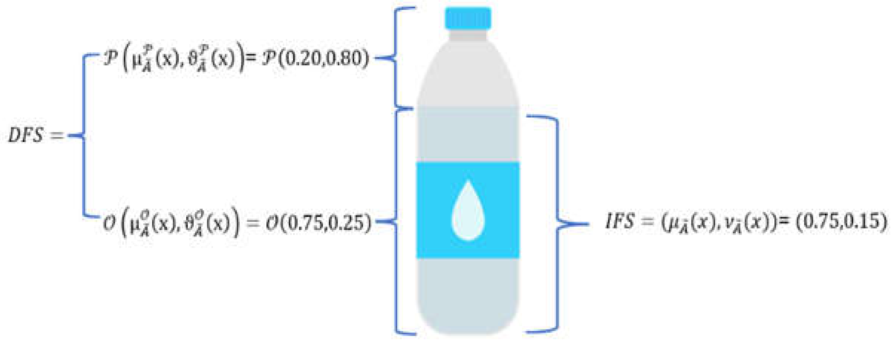
Figure 2.
One-at-a-time sensitivity analysis.
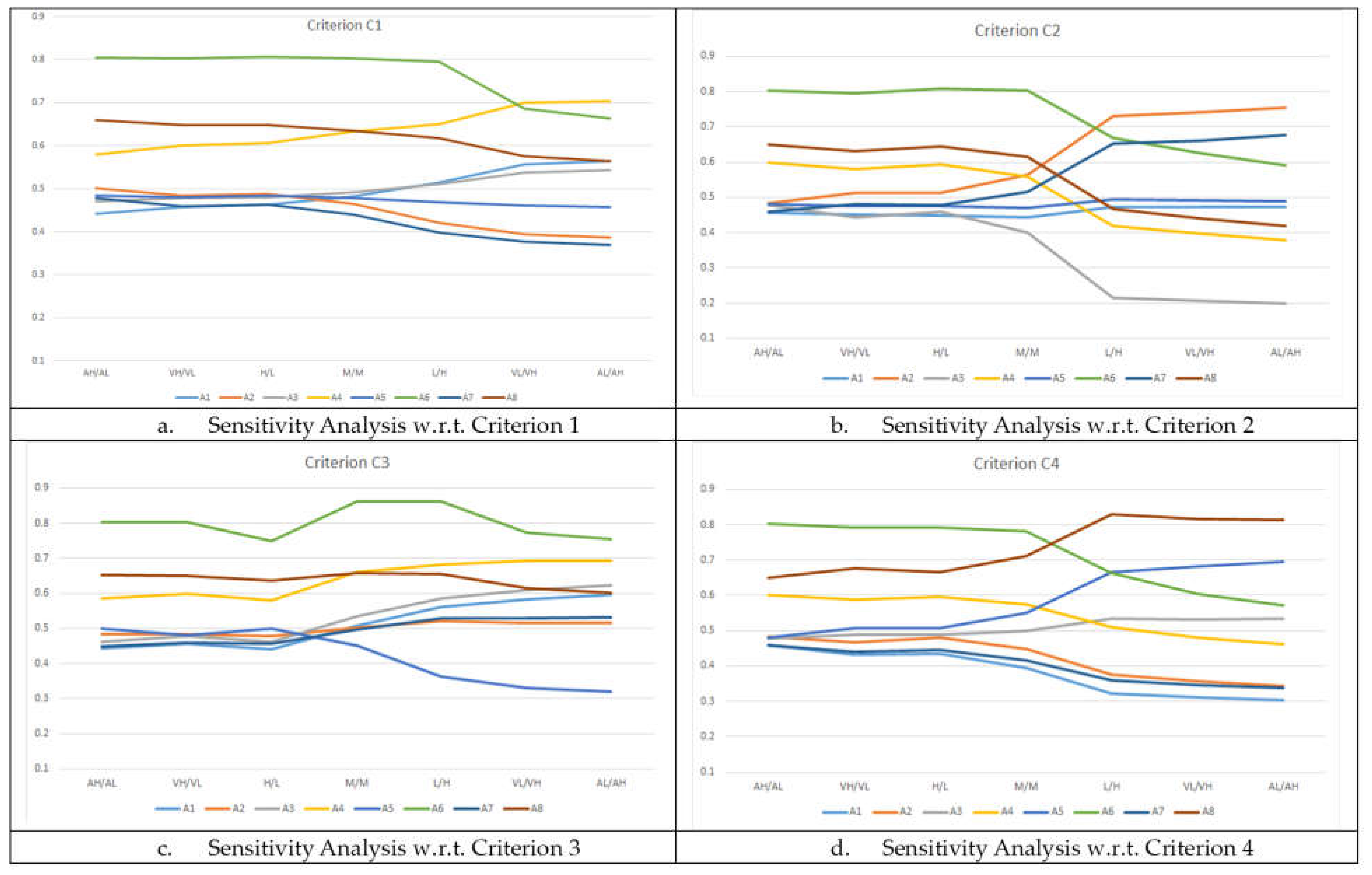
Table 2.
Expert linguistic evaluations.
| Expert-1 | C1. Delivery time | C2. Financial instability | C3. Reputation | C4. Quality | ||||
|---|---|---|---|---|---|---|---|---|
| F* | D** | F* | D** | F* | D** | F* | D** | |
| A1 | VL | VH | M | M | L | H | H | M |
| A2 | AH | AL | AL | AH | M | M | VH | VL |
| A3 | L | H | AH | AL | VL | VH | L | H |
| A4 | L | H | AH | AL | L | H | VH | VL |
| A5 | H | L | M | M | AH | AL | AL | AH |
| A6 | AH | AL | VH | VL | H | M | AH | VL |
| A7 | AH | AL | AL | AH | L | H | H | L |
| A8 | AH | AL | AH | AL | VH | VL | AL | AH |
| Expert-2 | C1. Delivery time | C2. Financial instability | C3. Reputation | C4. Quality | ||||
| F* | D** | F* | D** | F* | D** | F* | D** | |
| A1 | VL | VH | L | H | VL | VH | VH | L |
| A2 | VH | L | AL | AH | M | M | H | VL |
| A3 | M | H | VH | VL | VL | VH | L | H |
| A4 | VL | VH | AH | AL | L | H | VH | VL |
| A5 | H | L | H | L | AH | AL | VL | VH |
| A6 | H | L | VH | VL | H | M | VH | VL |
| A7 | VH | L | AL | AH | L | H | H | L |
| A8 | AH | AL | VH | VL | H | M | L | VH |
| Expert-3 | C1. Delivery time | C2. Financial instability | C3. Reputation | C4. Quality | ||||
| F* | D** | F* | D** | F* | D** | F* | D** | |
| A1 | L | M | H | M | VL | VH | VH | VL |
| A2 | AH | AL | AL | AH | M | M | VH | VL |
| A3 | L | H | VH | VL | VL | VH | L | H |
| A4 | L | H | VH | AL | L | H | VH | VL |
| A5 | H | L | L | H | AH | AL | AL | AH |
| A6 | H | VL | H | L | VH | L | VH | L |
| A7 | H | VL | L | H | L | L | VH | L |
| A8 | H | M | VH | AL | H | L | H | VL |
*F: Functional point of view, **D: Dysfunctional point of view.
Table 3.
Decomposed fuzzy representations of expert evaluations.
| Expert-1 | C1. Delivery time | C2. Financial instability | C3. Reputation | C4. Quality |
|---|---|---|---|---|
| A1 | ((0.2,0.8),(0.8,0.2)) | ((0.5,0.5),(0.5,0.5)) | ((0.35,0.65),(0.65,0.35)) | ((0.65,0.35),(0.5,0.5)) |
| A2 | ((0.95,0.05),(0.05,0.95)) | ((0.05,0.95),(0.95,0.05)) | ((0.5,0.5),(0.5,0.5)) | ((0.8,0.2),(0.2,0.8)) |
| A3 | ((0.35,0.65),(0.65,0.35)) | ((0.95,0.05),(0.05,0.95)) | ((0.2,0.8),(0.8,0.2)) | ((0.35,0.65),(0.65,0.35)) |
| A4 | ((0.35,0.65),(0.65,0.35)) | ((0.95,0.05),(0.05,0.95)) | ((0.35,0.65),(0.65,0.35)) | ((0.8,0.2),(0.2,0.8)) |
| A5 | ((0.65,0.35),(0.35,0.65)) | ((0.5,0.5),(0.5,0.5)) | ((0.95,0.05),(0.05,0.95)) | ((0.05,0.95),(0.95,0.05)) |
| A6 | ((0.95,0.05),(0.05,0.95)) | ((0.8,0.2),(0.2,0.8)) | ((0.65,0.35),(0.5,0.5)) | ((0.95,0.05),(0.2,0.8)) |
| A7 | ((0.95,0.05),(0.05,0.95)) | ((0.05,0.95),(0.95,0.05)) | ((0.35,0.65),(0.65,0.35)) | ((0.65,0.35),(0.35,0.65)) |
| A8 | ((0.95,0.05),(0.05,0.95)) | ((0.95,0.05),(0.05,0.95)) | ((0.8,0.2),(0.2,0.8)) | ((0.05,0.95),(0.95,0.05)) |
| Expert-2 | C1. Delivery time | C2. Financial instability | C3. Reputation | C4. Quality |
| A1 | ((0.2,0.8),(0.8,0.2)) | ((0.35,0.65),(0.65,0.35)) | ((0.2,0.8),(0.8,0.2)) | ((0.8,0.2),(0.35,0.65)) |
| A2 | ((0.8,0.2),(0.35,0.65)) | ((0.05,0.95),(0.95,0.05)) | ((0.5,0.5),(0.5,0.5)) | ((0.65,0.35),(0.2,0.8)) |
| A3 | ((0.5,0.5),(0.65,0.35)) | ((0.8,0.2),(0.2,0.8)) | ((0.2,0.8),(0.8,0.2)) | ((0.35,0.65),(0.65,0.35)) |
| A4 | ((0.2,0.8),(0.8,0.2)) | ((0.95,0.05),(0.05,0.95)) | ((0.35,0.65),(0.65,0.35)) | ((0.8,0.2),(0.2,0.8)) |
| A5 | ((0.65,0.35),(0.35,0.65)) | ((0.65,0.35),(0.35,0.65)) | ((0.95,0.05),(0.05,0.95)) | ((0.2,0.8),(0.8,0.2)) |
| A6 | ((0.65,0.35),(0.35,0.65)) | ((0.8,0.2),(0.2,0.8)) | ((0.65,0.35),(0.5,0.5)) | ((0.8,0.2),(0.2,0.8)) |
| A7 | ((0.8,0.2),(0.35,0.65)) | ((0.05,0.95),(0.95,0.05)) | ((0.35,0.65),(0.65,0.35)) | ((0.65,0.35),(0.35,0.65)) |
| A8 | ((0.95,0.05),(0.05,0.95)) | ((0.8,0.2),(0.2,0.8)) | ((0.65,0.35),(0.5,0.5)) | ((0.35,0.65),(0.8,0.2)) |
| Expert-3 | C1. Delivery time | C2. Financial instability | C3. Reputation | C4. Quality |
| A1 | ((0.35,0.65),(0.5,0.5)) | ((0.65,0.35),(0.5,0.5)) | ((0.2,0.8),(0.8,0.2)) | ((0.8,0.2),(0.2,0.8)) |
| A2 | ((0.95,0.05),(0.05,0.95)) | ((0.05,0.95),(0.95,0.05)) | ((0.5,0.5),(0.5,0.5)) | ((0.8,0.2),(0.2,0.8)) |
| A3 | ((0.35,0.65),(0.65,0.35)) | ((0.8,0.2),(0.2,0.8)) | ((0.2,0.8),(0.8,0.2)) | ((0.35,0.65),(0.65,0.35)) |
| A4 | ((0.35,0.65),(0.65,0.35)) | ((0.8,0.2),(0.05,0.95)) | ((0.35,0.65),(0.65,0.35)) | ((0.8,0.2),(0.2,0.8)) |
| A5 | ((0.65,0.35),(0.35,0.65)) | ((0.35,0.65),(0.65,0.35)) | ((0.95,0.05),(0.05,0.95)) | ((0.05,0.95),(0.95,0.05)) |
| A6 | ((0.65,0.35),(0.2,0.8)) | ((0.65,0.35),(0.35,0.65)) | ((0.8,0.2),(0.35,0.65)) | ((0.8,0.2),(0.35,0.65)) |
| A7 | ((0.65,0.35),(0.2,0.8)) | ((0.35,0.65),(0.65,0.35)) | ((0.35,0.65),(0.35,0.65)) | ((0.8,0.2),(0.35,0.65)) |
| A8 | ((0.65,0.35),(0.5,0.5)) | ((0.8,0.2),(0.05,0.95)) | ((0.65,0.35),(0.35,0.65)) | ((0.65,0.35),(0.2,0.8)) |
Table 4.
Aggregated expert evaluations.
| Aggregated | C1. Delivery time | C2. Financial instability | C3. Reputation | C4. Quality |
|---|---|---|---|---|
| A1 | ((0.26,0.75),(0.71,0.29)) | ((0.51,0.5),(0.55,0.45)) | ((0.25,0.76),(0.76,0.24)) | ((0.75,0.23),(0.35,0.65)) |
| A2 | ((0.9,0.04),(0.15,0.85)) | ((0.05,0.95),(0.95,0.05)) | ((0.5,0.5),(0.5,0.5)) | ((0.75,0.23),(0.2,0.8)) |
| A3 | ((0.4,0.6),(0.65,0.35)) | ((0.85,0.08),(0.16,0.84)) | ((0.2,0.8),(0.8,0.2)) | ((0.35,0.65),(0.65,0.35)) |
| A4 | ((0.3,0.7),(0.7,0.3)) | ((0.9,0.03),(0.05,0.95)) | ((0.35,0.65),(0.65,0.35)) | ((0.8,0.2),(0.2,0.8)) |
| A5 | ((0.65,0.35),(0.35,0.65)) | ((0.49,0.49),(0.53,0.47)) | ((0.95,0.05),(0.05,0.95)) | ((0.1,0.91),(0.92,0.08)) |
| A6 | ((0.75,0.1),(0.21,0.79)) | ((0.75,0.22),(0.26,0.74)) | ((0.7,0.29),(0.44,0.56)) | ((0.85,0.08),(0.26,0.74)) |
| A7 | ((0.8,0.08),(0.21,0.79)) | ((0.17,0.87),(0.89,0.11)) | ((0.35,0.65),(0.55,0.45)) | ((0.7,0.29),(0.35,0.65)) |
| A8 | ((0.85,0.03),(0.27,0.73)) | ((0.85,0.08),(0.1,0.9)) | ((0.7,0.27),(0.36,0.64)) | ((0.37,0.71),(0.77,0.23)) |
Table 5.
Weighted aggregated expert evaluations.
| C1. Delivery time | C2. Financial instability | C3. Reputation | C4. Quality | |
|---|---|---|---|---|
| A1 | ((0.21,0.8),(0.18,0.82)) | ((0.48,0.53),(0.05,0.95)) | ((0.2,0.81),(0.19,0.81)) | ((0.71,0.27),(0.05,0.95)) |
| A2 | ((0.72,0.23),(0.09,0.91)) | ((0.05,0.95),(0.05,0.95)) | ((0.4,0.6),(0.17,0.83)) | ((0.71,0.27),(0.04,0.96)) |
| A3 | ((0.32,0.68),(0.18,0.82)) | ((0.81,0.13),(0.04,0.96)) | ((0.16,0.84),(0.19,0.81)) | ((0.33,0.67),(0.05,0.95)) |
| A4 | ((0.24,0.76),(0.18,0.82)) | ((0.85,0.08),(0.03,0.97)) | ((0.28,0.72),(0.18,0.82)) | ((0.76,0.24),(0.04,0.96)) |
| A5 | ((0.52,0.48),(0.15,0.85)) | ((0.47,0.51),(0.05,0.95)) | ((0.76,0.24),(0.04,0.96)) | ((0.09,0.92),(0.05,0.95)) |
| A6 | ((0.6,0.28),(0.11,0.89)) | ((0.71,0.25),(0.04,0.96)) | ((0.56,0.43),(0.16,0.84)) | ((0.81,0.13),(0.04,0.96)) |
| A7 | ((0.64,0.26),(0.11,0.89)) | ((0.16,0.88),(0.05,0.95)) | ((0.28,0.72),(0.17,0.83)) | ((0.67,0.32),(0.05,0.95)) |
| A8 | ((0.68,0.22),(0.13,0.87)) | ((0.81,0.13),(0.03,0.97)) | ((0.56,0.42),(0.15,0.85)) | ((0.35,0.72),(0.05,0.95)) |
Table 6.
Consistency Index.
| C1. Delivery time | C2. Financial instability | C3. Reputation | C4. Quality | |
|---|---|---|---|---|
| A1 | 0.288 | 0.526 | 0.282 | 0.767 |
| A2 | 0.909 | 0.097 | 0.523 | 0.763 |
| A3 | 0.427 | 0.867 | 0.239 | 0.381 |
| A4 | 0.334 | 0.896 | 0.381 | 0.802 |
| A5 | 0.663 | 0.526 | 0.928 | 0.137 |
| A6 | 0.784 | 0.77 | 0.719 | 0.87 |
| A7 | 0.825 | 0.189 | 0.381 | 0.718 |
| A8 | 0.861 | 0.862 | 0.722 | 0.361 |
Table 7.
Score Index values.
| C1. Delivery time | C2. Financial instability | C3. Reputation | C4. Quality | |
|---|---|---|---|---|
| A1 | 0.187 | 0.404 | 0.181 | 0.678 |
| A2 | 0.87 | 0.054 | 0.399 | 0.676 |
| A3 | 0.306 | 0.808 | 0.149 | 0.264 |
| A4 | 0.224 | 0.863 | 0.264 | 0.729 |
| A5 | 0.555 | 0.4 | 0.918 | 0.078 |
| A6 | 0.691 | 0.679 | 0.619 | 0.81 |
| A7 | 0.747 | 0.115 | 0.264 | 0.618 |
| A8 | 0.8 | 0.806 | 0.62 | 0.254 |
Table 8.
Positive and Negative ideal solutions.
| C1. Delivery time | C2. Financial instability | C3. Reputation | C4. Quality | |
|---|---|---|---|---|
| PIS | ((0.86,0.09),(0.04,0.96)) | ((0.85,0.08),(0.03,0.97)) | ((0.9,0.1),(0.03,0.97)) | ((0.81,0.13),(0.04,0.96)) |
| NIS | ((0.24,0.77),(0.05,0.95)) | ((0.05,0.95),(0.05,0.95)) | ((0.19,0.81),(0.05,0.95)) | ((0.09,0.92),(0.05,0.95)) |
Table 9.
Distances, CC Indexes and Rank of the alternatives.
| D to PIS | D to NIS | CC index | Rank | |
|---|---|---|---|---|
| A1 | 0.723 | 0.543 | 0.429 | 8 |
| A2 | 0.672 | 0.67 | 0.499 | 5 |
| A3 | 0.716 | 0.596 | 0.454 | 7 |
| A4 | 0.588 | 0.768 | 0.566 | 3 |
| A5 | 0.635 | 0.647 | 0.505 | 4 |
| A6 | 0.213 | 0.885 | 0.806 | 1 |
| A7 | 0.678 | 0.596 | 0.468 | 6 |
| A8 | 0.41 | 0.811 | 0.664 | 2 |
Disclaimer/Publisher’s Note: The statements, opinions and data contained in all publications are solely those of the individual author(s) and contributor(s) and not of MDPI and/or the editor(s). MDPI and/or the editor(s) disclaim responsibility for any injury to people or property resulting from any ideas, methods, instructions or products referred to in the content. |
© 2023 by the authors. Licensee MDPI, Basel, Switzerland. This article is an open access article distributed under the terms and conditions of the Creative Commons Attribution (CC BY) license (http://creativecommons.org/licenses/by/4.0/).
Copyright: This open access article is published under a Creative Commons CC BY 4.0 license, which permit the free download, distribution, and reuse, provided that the author and preprint are cited in any reuse.


