
Submitted:
15 June 2023
Posted:
16 June 2023
You are already at the latest version
Abstract
Channel estimation is an important module to enhance the performance of orthogonal frequency division multiplexing (OFDM) systems. However, the presence of a large amount of noise in multipath fading time-varying channels significantly affects the channel estimation accuracy and thus the recovery quality of the received signals. Therefore, this paper proposes a double-threshold (DT) channel estimation method based on adaptive frame statistics (AFS). The method first adaptively determines the number of statistical frames based on the temporal correlation of the received signals, and preliminarily detects the channel structure by analyzing the distribution characteristics of multipath sampling points and noise sampling points during adjacent frames. Subsequently, a multi-frame averaging technique is used to expand the distinction between multipath and noise sampling points. Finally, the DT is designed to better recover the channel based on the preliminary detection results. Simulation results show that the proposed adaptive frame statistics-double-threshold (AFS-DT) channel estimation method is effective and has better performance compared with many existing channel estimation methods.
Keywords:
channel estimation
; orthogonal frequency division multiplexing (OFDM)
; adaptive frame statistics (AFS)
; double-threshold (DT)
1. Introduction
Orthogonal frequency division multiplexing (OFDM) technology is extensively employed in modern communication systems due to its exceptional performance and high spectral efficiency [1,2]. By inserting a cyclic prefix (CP) which is greater than the maximum delay extension of the multipath channel among adjacent OFDM symbols as the guard interval (GI), it not only eliminates inter-symbol interference (ISI) but also greatly simplifies the design of the frequency domain equalizer [3]. To recover the signals accurately at the receiver, channel estimation is essential. The current channel estimation methods for OFDM systems can be divided into three categories: blind channel estimation [4], semi-blind channel estimation [5], and pilot-based channel estimation [6]. Although blind and semi-blind channel estimation methods have higher spectral efficiency, their high computational complexity is not ideal in practical applications. The pilot-based channel estimation methods are often preferred due to their reliability and simplicity. Usually the pilots are inserted in block-type [7], comb-type [8], or scatter-type [9]. In the block-type arrangement, the pilots appear in a few OFDM symbols of all subcarriers. In the comb-type arrangement, the pilots appear in a few subcarriers of all OFDM symbols. In the scatter-type arrangement, the pilots appear in a few subcarriers of a few OFDM symbols. Therefore, the number of pilots in the scatter-type is less than that in the block-type and comb-type. However, the comb-type pilots can better recover the channel state information (CSI) in time-varying channels [10]. Therefore, this paper focuses on the channel estimation techniques based on comb-type pilots. Figure 1 gives the mainstream channel estimation methods based on comb-type pilots in OFDM systems, which are error square minimization, multi-frame averaging, compressed sensing (CS), and threshold denoising. The threshold denoising methods in the red dashed box and the multi-frame averaging methods in the blue dashed box in the figure are the theoretical sources of the proposed method in this paper.
At the receiver, the channel is estimated using the known and received pilots. There are many conventional channel estimation techniques such as least square (LS) method [11], minimum mean square error (MMSE) method [12], and linear MMSE (LMMSE) method [13]. The LS method is the simplest channel estimation method and has been widely used for many years. However, it ignores the effect of noise, which reduces its channel estimation accuracy greatly. The MMSE method uses priori knowledge in the form of second-order statistics of the channel and has better estimation performance, but it involves matrix inverse operations and has high computational complexity. The LMMSE method is a simplification of the MMSE method. Although it reduces the computational complexity, it still requires prior channel knowledge to calculate the autocorrelation matrix of the channel. The LS-based channel estimator is simple to implement and does not require prior knowledge of the channel. To enhance its performance, numerous denoising strategies have been proposed in existing literatures. Wu et al. [14] proposed a weighted averaging channel estimation method according to the temporal correlation of wireless channels. Based on the LS estimation, the channel coefficients of two adjacent OFDM symbols are weighted averaged. The noise is better suppressed under this method, but it is not effective in dynamic channels. Zettas et al. [15] adaptively adjusted the buffer according to the Doppler shift, and thus the average number of OFDM frames is determined to adapt to dynamic channels. Based on this, Zhang et al. [16] considered the effect of signal-to-noise ratio (SNR) on the average number of OFDM frames and proposed a more reasonable multi-frame weighted averaging scheme. However, the multi-frame averaging technique causes Doppler distortion in dynamic channels. In fast time-varying channel environments, the performance loss from multi-frame averaging could be higher than the performance gain of noise suppression. Therefore, the methods proposed by Zettas et al. [15] and Zhang et al. [16] still have some limitations.
For some bandwidth wireless channels, the channel impulse response (CIR) often exhibits a sparse structure due to delay differences and relatively high sampling rates. CS algorithms have been successfully applied to the recovery of sparse channel support sets. They are mainly classified into convex optimization [17] and greedy optimization [18]. Convex optimization mainly uses basis pursuit (BP) [19] to solve the parametric minimization problem. Its reconstruction accuracy for sparse channel is high, but it is not applicable to real-time systems and has high complexity. In contrast to convex optimization which sets the objective function to minimize, greedy optimization determines the location of the non-zero sampling points of the sparse channel by multiple iterations. Orthogonal matching pursuit (OMP) [20], block OMP (BOMP) [21], and compressive sampling matching pursuit (CoSaMP) [22] are the most commonly used CS algorithms. Jiang et al. [23] proposed a separable CoSaMP (SCoSaMP) algorithm based on the introduction of backtracking idea. It effectively improves the channel estimation accuracy while reducing the complexity. For some scenarios where the channels satisfy the joint sparse model (JSM), simultaneous OMP (SOMP) [24] algorithm effectively utilizes the joint sparse property to obtain a better sparse channel reconstruction performance. Based on this, Wang et al. [25] proposed an improved SOMP algorithm to achieve ordinary channel taps detection and dynamic channel taps pursuit. Its channel recovery performance is significantly improved under the sparse channel model with the same partial support sets. However, the above CS algorithms [20,21,22,23,24,25] usually require a large number of iterations to reduce the approximation error, which brings high complexity. Moreover, channel estimation methods based on CS algorithms require known number of channel common support sets to achieve optimal performance, which limits their scope of application.
Threshold-based channel estimation methods have lower complexity than those based on CS algorithms and mostly do not require known number of channel common support sets. They typically use the LS method to obtain the initial CIR. Then, the amplitude of each sample point is compared with a given threshold to determine the multipath sample points. The performance of channel CIR support sets recovery depends heavily on the setting of detection thresholds. Most conventional spectrum sensing methods use a fixed threshold to distinguish the multipath and noise sampling points. For example, Kang et al. [26] proposed a double noise variance threshold (DNT) by calculating the noise variance from sampling points outside the CP. Tripta et al. [27] implemented the estimation of noise standard deviation by wavelet decomposition and set it directly as the threshold. However, it is difficult to guarantee the noise removal rate by using a fixed threshold. Its performance degrades faster, especially when the noise power fluctuates. Xu et al. [28] proposed a piecewise suboptimal threshold (PSOT) for selecting the most significant samples (MSSs) in the estimated CIR. This threshold is set by setting the first-order derivative of the mean square error (MSE) to zero to filter out the possible noise samples in the MSSs as much as possible. Zhang et al. [29] proposed a channel estimation method based on the combination of adaptive multi-frame averaging and improved MSE optimal threshold (IMOT). In this method, most of the noise is suppressed without significantly increasing the computational complexity. To obtain a more desirable performance, both PSOT and IMOT require priori channel sparsity for assistance, which is often difficult to obtain in practice. In a completely unknown channel environment, Sure et al. [30] proposed a weighted noise threshold (WNT) by introducing a modified interpretation of the hypothesis testing problem. To some extent, the MSE degradation problem caused by the estimation of priori channel information is overcome. Bahonar et al. [31] proposed a sparse recovery method based on sparse domain smoothing. It is mainly divided into three parts: time domain residue computation, sparsity domain smoothing, and adaptive thresholding sparsifying. Its performance of channel recovery is improved considerably at the expense of certain complexity. However, the performance of existing threshold denoising methods is often unsatisfactory in low SNR range. The reason is that regardless of how the threshold is selected in low SNR range, there is the problem of misclassification of multipath sampling points with lower energy and noise sampling points with higher energy.
To improve the accuracy of channel estimation in fast time-varying channels and ensure computational complexity, this paper proposes a double-threshold (DT) estimation channel method based on adaptive frame statistics (AFS) by utilizing the sparsity and temporal correlation of wireless channels. Its performance in terms of normalized mean square error (NMSE), channel structure correctness detection rate (SCDR), and bit error rate (BER) is better than many existing threshold denoising methods in low SNR range. The main novelties and contributions are as follows:
- (1)
- The temporal correlation of the received signals is used to analyze the time-varying characteristics of the channel, so that the number of OFDM statistical frames can be determined adaptively.
- (2)
- The channel estimation accuracy is further improved by designing the DT based on the preliminary detection results combined with the distribution characteristics of the sampling points.
- (3)
- To fully utilize the cache resources and improve the performance of DT, a multi-frame averaging technique is used to expand the distinction between multipath and noise sampling points after the preliminary statistics.
The rest of this paper is organized as follows. Section 2 presents the system model. Section 3 derives the proposed AFS-DT channel estimation method in detail. Experimental results of the proposed method and other conventional methods are given in Section 4, and the computational complexity of the different methods is compared and analyzed. Section 5 summarizes the research work.
2. System Model
It is supposed that one OFDM symbol is transmitted in one frame in this paper. Figure 2 shows the CP-OFDM system model using the proposed AFS-DT channel estimation method. The main research work of this paper is shown in the red dashed box in the figure. At the transmitter, the input binary bits are grouped and mapped by 4-quadrature amplitude modulation (4QAM). After inserting the comb-type pilots with uniform interval and length , a serial to parallel (S/P) transformation is performed. The inverse fast Fourier transform (IFFT) block converts the data with N rows into the time-domain signals, where N is the number of subcarriers. Then, the CP of length is added to the time-domain OFDM symbols, which should be larger than the maximum channel delay extension L (in terms of samples) [32]. The transmitted signals will pass through the multipath fading channel with additive white Gaussian noise (AWGN) after parallel to serial (P/S) transformation.
At the receiver, it is assumed to be perfectly synchronized with the transmitter. The CP is removed after the S/P transformation. The fast Fourier transform (FFT) output of the pilot symbols is expressed as:
where and represent the received and transmitted pilot of the mth subcarrier in the kth OFDM symbol, respectively. is the true channel frequency response (CFR), and represents AWGN.
The channel estimation module uses the LS method to obtain the CFR , which can be expressed as:
The CFR is transformed to the time domain by the -point IFFT. Considering the sparsity of the wireless channels, the CIR can be specifically expressed as:
where is the true CIR support sets, which can be considered as the position of the multipath sampling points in interval sampling channels. is the true CIR at the multipath sampling points, which can be modeled as a complex Gaussian random variable with mean 0 and variance in Rayleigh fading channels. is the complex AWGN with mean 0 and variance . Since and are independent of each other, also conforms to the complex Gaussian distribution. Therefore, the random variable is distributed as:
Since AWGN is ignored in the LS method, the channel estimation accuracy will be further improved in the AFS-DT denoising module, which will be described in detail in Section 3. Finally, the transmitted binary bits are obtained by the 4QAM demodulation method.
3. The Proposed Method
The existing threshold denoising methods have limitations in low SNR range. Therefore, an AFS-DT based channel estimation method is proposed in this paper. First, the channel structure is preliminarily determined by multi-frame statistics based on the distribution characteristics of multipath sampling points and noise sampling points. The number of statistical frames P is determined adaptively according to the temporal correlation of the received signals, and the derivation process will be described in detail in Section 3.2. A multi-frame averaging technique is then used to expand the distinction between multipath and noise sampling points. Finally, a cost factor is introduced to design a denoising threshold that minimizes the overall error cost, and another threshold is introduced to supplement multipath.
Perform P-frame statistics on the CIR obtained by LS estimation. Let the number of times the real part of the mth sampling point appears in the statistical intervals and be and , respectively. Similarly, let the number of times the imaginary part of the mth sampling point appears in the statistical intervals and be and , respectively. The counting process can be specifically expressed as [33]:
where denotes the operation of counting. and denote the operations of taking the real and imaginary parts, respectively.
Next, define the variable :
where denotes the operation of taking the maximum value.
In the time-varying channels, there exists a certain degree of correlation among adjacent OFDM symbols. Since the probability density function (PDF) of noise conforms to the zero-mean complex Gaussian distribution, it is known from the statistical properties of noise that if the mth sampling point is a pure noise sampling point, the number of times its real or imaginary part appears in the intervals and is similar. It can be considered that . In practical communication environments, the power of multipath in the channel is much greater than the power of noise. Considering the correlation among adjacent OFDM frames, if the mth point is a multipath sampling point, the number of times its real or imaginary part appears in the statistical intervals and approximates the number of statistical frames, i.e. . Therefore, the preliminary channel structure detection matrix can be expressed as:
where the value of 1 represents a multipath sampling point, and the value of 0 represents a noise sampling point.
Due to the extreme randomness of statistics and the time-varying nature of the channel, there are still misclassifications of noise as multipath and multipath as noise. Therefore, further optimization is needed. P-frame averaging of the CIR can be expressed as:
The channel information of adjacent OFDM frames is still similar due to the temporal correlation of the channel. It can be considered that . That is, the true multipath power after averaging is approximately equal to the unaveraged true multipath power . The multipath power after superimposed noise becomes , and the noise power is . Therefore, the CIR after averaging conforms to the following complex Gaussian distribution:
Combining (4) and (12), the change in the distinction between multipath sampling points and noise sampling points can be specifically expressed as:
It can be seen that by averaging the adjacent P-frame OFDM symbols, the distinction in energy between multipath sampling points and noise sampling points is approximately expanded by a factor of P. Unlike the purpose of conventional multi-frame averaging, it is not directly used to average the CIR for noise suppression. This is because multi-frame averaging in dynamic channels distorts the channel coefficients at the multipath sampling points, which means that is not rigorous and even causes errors.
The square of the envelope of the CIR after averaging gives , which represents the power and follows an exponential distribution. The cumulative distribution functions (CDF) and of multipath power and noise power can be specifically expressed as:
When the power at the mth subcarrier in the kth OFDM frame is less than the denoising threshold , it is considered as a noise sampling point, and vice versa as a multipath sampling point. According to the nature of the CDF, when , the multipath error removal probability is and the noise correct removal probability is . Therefore, the probabilities of missed alarm (MA) and false alarm (FA) are and , respectively. The overall error cost can be expressed as:
where is the introduced FA cost factor, the specific value of which will be given in Section 4.2. To obtain the optimal denoising threshold, the first order derivative of for the overall error cost can be expressed as:
Let the first order derivative be equal to zero, and the denoising threshold for finding the minimum error cost can be specified as:
Since the multipath power is usually much larger than the noise power , the essence of this denoising threshold is multiple of the noise power corresponding to the kth frame. Based on this, the threshold for supplementing multipath can be expressed as:
The preliminary channel structure detection matrix is further optimized with the denoising threshold and the supplementary multipath threshold . Searching for possible noise sampling points among the originally judged multipath sampling points, the selection principle is less than the denoising threshold set in the current frame. Searching for possible multipath sampling points among the originally judged noise sampling points, the selection principle is greater than the supplementary multipath threshold set in the current frame. The final channel structure detection matrix can be specifically expressed as:
where and are the CIRs of multipath and noise after preliminary detection, respectively.
Based on the final channel structure detection matrix for time-domain denoising, the final CIR can be expressed as:
3.1. Estimation of Multipath Power and Noise Power
From (18) and (19), the optimal threshold requires known multipath power and noise power . Next, the and will be estimated based on the preliminary detection results.
The CIR at all multipath sampling points is obtained from the CIR and the preliminary channel structure detection matrix , which is expressed as:
Based on the CIR with multipath energy only, the average multipath power of the kth OFDM frame is calculated, which can be expressed as:
where denotes summation by column.
The CIR at all noise sampling points is obtained from the CIR and the preliminary channel structure detection matrix , which is expressed as:
where denotes an all-one matrix with the same dimension as . The noise power of the kth OFDM frame can be expressed as:
where denotes the operation of taking the median by column.
3.2. Determination of P
For an OFDM system with a baseband bandwidth of B, let the duration of a time-domain OFDM symbol (containing CP) be , which is specified as:
Assuming the number of frames for frame statistics is P, the duration of P-frame OFDM symbols can be expressed as:
To ensure the reliability of preliminary statistical results, there should be a strong correlation among the OFDM frames used for statistics. That is, the channel has a small variation in the duration . Therefore, should be smaller than the coherence time of the channel, i.e.:
where is the buffer factor and the value is greater than 1, and it is selected as for the proposed AFS-DT method. Meanwhile, the coherence time of the channel can be defined as [34]:
where is the Doppler shift. Assuming that the speed of the user equipment (UE) is v, the speed of light is c, and the system carrier frequency is . When the incident signals run in the same direction as the UE, can be expressed as [35]:
Combining (27), (28), and (29), P can be determined as:
where stands for rounding down to ensure inter-frame correlation. From (31), it can be seen that the estimation of the Doppler shift is essential for the adaptive determination of the statistical frame number P. Under Rayleigh fading channel models, the autocorrelation function of the time-domain received signals can be expressed as a first class zero-order Bessel function [35]:
where is the difference in the number of OFDM symbols. On the other hand, the autocorrelation function can be calculated directly from the time-domain received signals as:
where denotes the kth frame of OFDM symbols received in the time domain. denotes the operation of conjugate transpose. Next, the first negative value of is found according to (33) and let be . Then, the first zero crossing point is determined by linear interpolation, which can be specified as:
Since the first zero crossing point of the first class zero-order Bessel function is , there is when . The resulting estimate of the Doppler shift can be achieved specifically as [16]:
4. Simulation Results
To evaluate the effectiveness of the proposed method in this paper, this section conducts simulations on the NMSE, SCDR, and BER of the AFS method and the further optimized AFS-DT method. Several conventional methods are also simulated and compared, which include DNT [26], WNT [30], and IMOT [29]. The performance metrics and simulation environments including the channel models and system parameters are given in Section 4.1. For the proposed AFS-DT method, the specific determination process of the FA cost factor is given in Section 4.2. For the WNT method, the weight factor q is taken as . For the IMOT method, the prior probability of multipath sampling points is taken as the local sparsity level (LSL) . This section also simulates the channel estimation performance for two ideal cases, namely known true channel structure and noise-free interference. Finally, the computational complexity of the different channel estimation methods is analyzed and compared in Section 4.5.
4.1. Simulation Environments and Performance Metrics
The channel models used are two new models from the Finnish Wing-TV test project [15]: the vehicular urban (VU) and the motorway rural (MR). These channels are all Rayleigh channels with the multipath number of 12, whose power delay profiles (PDP) are shown in Table 1. The main simulation parameters of the OFDM system are shown in Table 2. There are 1200 subcarriers, of which the CP occupies 240 subcarriers. Therefore, the total number of pilot subcarriers and data subcarriers is . The number of pilot subcarriers is by using the comb-type pilots with an interval of 3. In the dynamic multipath channel environments, the system carrier frequency is set to 800 MHz. The speeds of UE in VU and MR are set to 40 km/h and 100 km/h, respectively. The finally simulation results are obtained by averaging totally 1000 trail runs.
In this paper, the channel estimation performance is evaluated in terms of NMSE, SCDR, and BER, which can be defined as (37), (38), and (39), respectively:
where denotes the operation of taking the mean value. and represent the true CIR and the CIR obtained by various channel estimation methods, respectively. means summing all elements of the matrix. and represent the true channel structure detection matrix and the channel structure detection matrix obtained by various threshold channel estimation methods, respectively. and are the number of error bits and the total number of bits which are sent in the transmitter, respectively.
4.2. Determination of
Since most of the sampling points in an OFDM frame are noise sampling points, the value of should theoretically be within the interval . To verify the theoretical reasoning and find the optimal , the NMSE simulation curves for the VU channel with UE speed of 40 km/h and the MR channel with UE speed of 100 km/h when are shown in Figure 3a and Figure 3b , respectively. The trends of the simulation curves are similar in both channels, but the difference in NMSE among different values is more obvious in the MR channel. This is because the fast time-varying characteristics of the MR channel lead to a high probability of misclassification in the AFS method, and the DT can improve the channel estimation performance more significantly. Therefore, the result of the MR channel is described in detail as an example.
As shown in Figure 3b, the value of NMSE becomes smaller as increases when . From (18) and (19), it can be seen that as becomes larger, the denoising threshold becomes larger while the complementary multipath threshold becomes smaller, which makes the DT have better denoising and supplementary multipath performance. It also further verifies the theoretical reasoning that the optimal value is taken within the interval . When , the value of NMSE is still smaller when takes a larger value in the relatively high SNR range, but the performance improvement is not significant. Moreover, when or , the NMSE will sharply deteriorate in the lower SNR range. This is because too large causes the denoising threshold to incorrectly remove some multipath sampling points, while the supplementary multipath threshold also incorrectly supplements some noise sampling points. Therefore, is finally selected for the experiment in this section.
4.3. Analysis of NMSE and SCDR
Since both NMSE and SCDR reflect the degree of channel recovery to some extent, this subsection will simulate and analyze them together. The NMSE and SCDR of different channel estimation methods for the VU channel with UE speed of 40 km/h are shown in Figure 4a and Figure 4b, respectively. The NMSE and SCDR of different channel estimation methods for the MR channel with UE speed of 100 km/h are shown in Figure 5a and Figure 5b, respectively.
As shown in Figure 4a, the NMSE of all seven methods decreased with the increase of SNR. The proposed AFS-DT method has the best NMSE in the overall SNR range in addition to the ideal method with known true channel structure. The AFS method without further structural optimization shows suboptimal performance in the lower SNR range. It outperforms the ideal method with known true channel structure. This is because in the case of very low SNR, there are multipath sampling points with low multipath energy but high superimposed noise energy. The AFS method will judge these sampling points as noise and remove them. Compared with Figure 5a, the AFS-DT method in Figure 4a has a slightly lower performance gain compared with the conventional methods. The reason is that the number of statistical frames becomes smaller and the noise removal rate is lower to ensure the reliability of the preliminary channel structure detection under the MR channel.
As shown in Figure 4b, the SCDR of all five methods becomes larger with the increase of SNR. Among them, the performance of DNT method is the worst and the change with SNR is flat. This is because DNT is a fixed threshold and does not change adaptively as the SNR changes. When the SNR is 0 dB, the SCDR of the proposed AFS-DT method is improved by , , and compared with the DNT, WNT, and IMOT methods, respectively. As shown in Figure 5b, when the SNR is 0 dB, the SCDR of AFS-DT method is improved by , , and compared with the DNT, WNT, and IMOT methods, respectively.
As shown in Figure 4a,b, the performance of the AFS method compared with other conventional methods in terms of NMSE and SCDR does not exactly correspond in the overall SNR range. For example, at the SNR of 10 dB, the SCDR of AFS method is better than IMOT method, but the NMSE is lower than IMOT method. The same phenomenon is observed in Figure 5a compared with Figure 5b. The reason is that AFS method has a high noise removal rate in the high SNR range, but there is still a multipath sampling points misclassification problem, while the NMSE of IMOT method is basically caused by the unremoved noise.
4.4. Analysis of BER
The BER of the VU channel with UE speed of 40 km/h and the MR channel with UE speed of 100 km/h are shown in Figure 6 and Figure 7, respectively. To more clearly show the BER differences among the different methods, the part of each figure shown in the black dashed box has been enlarged.
As shown in Figure 6, the BER of all channel estimation methods gradually improves as the SNR increases. The reason is that as the SNR increases, the interference of the AWGN in the channel to the transmitted signals diminishes and the channel estimation accuracy improves. Except for the two ideal cases, AFS-DT method still shows the best performance in the overall SNR range compared with the conventional methods. In the lower SNR range, it also outperforms channel estimation method with known true channel structure. Figure 7 also shows similar experimental results. In Figure 6, when BER is , the SNR gains of the AFS-DT method compared with the DNT, WNT, and IMOT methods are about 1.90 dB, 0.30 dB, and 0.17dB. In Figure 7, when BER is , the SNR gains of the AFS-DT method compared with the DNT, WNT, and IMOT methods are about 1.80 dB, 0.25 dB, and 0.10 dB.
4.5. Analysis of Computational Complexity
The computational complexity of the proposed AFS and AFS-DT methods and the conventional methods is shown in Table 3. For intuitive presentation, all methods consider only complex multiplication operations in one frame of OFDM symbols.
For the AFS method, the statistical complexity can be ignored and only interpolation is required. Its computational complexity is . For the AFS-DT method, -point IFFT is first performed on the CFR at the pilots obtained by the LS method. Its computational complexity is . Then, the DT is calculated. It mainly includes the calculations of multi-frame averaging, multipath power, and noise power, corresponding to (11), (23), and (25), respectively. Their computational complexity is approximately and belongs to the same order of magnitude. The computational complexity of (18) and (19) can be ignored since the DT is computed only once in one frame of OFDM symbols. In addition, the determination of P in (36) needs to be computed only once for a given channel and can also be ignored. Finally, the N-point FFT of the CIR after DT optimization is performed to achieve the estimation of the CFR at the data subcarriers. Its computational complexity is . Since , it can be considered that . In summary, the computational complexity of the AFS-DT method is approximately .
As shown in Table 3, the computational complexity of the proposed AFS-DT method is in the same order of magnitude as the DNT and WNT methods, which is lower than the IMOT method. Since both LS and AFS methods do not require time domain operations, only interpolation is required and their complexity is minimal. Overall, the AFS-DT method greatly improves the channel estimation accuracy with reasonable computational complexity.
5. Conclusions
To achieve low complexity and high accuracy channel estimation under fast time-varying channels, a double-threshold channel estimation method based on adaptive frame statistics is proposed. The method is able to adapt to time-varying channels by adaptively determining the number of statistical frames based on the received signals. In addition, to further improve the accuracy of channel estimation, a multi-frame averaging technique is used to expand the difference between the multipath sampling points and the noise sampling points.
Simulation results show that the channel estimation accuracy of the proposed AFS-DT method is better than LS, DNT, WNT, and IMOT methods. At the same time, the method has a low computational complexity and is easy to implement. It has broad application prospects in the fields of optical communication [36], digital broadcasting [37], and satellite communication [38].
Author Contributions
C.S.: Investigation, Conceptualization, Methodology, Software, Validation, Writing—original draft, Writing—review and editing. X.Z.: Conceptualization, Writing—review and editing, Supervision, Project administration. C.W.: Investigation, Resources, Writing—review and editing. Z.Y.: Software, Writing—review and editing.
Funding
This work was supported in part by the Shandong Provincial Natural Science Foundation (Nos. ZR2022MF256, ZR2020MF008), in part by the Joint Fund of Shandong Provincial Natural Science Foundation (No. ZR2021LZH003), in part by the Scientific Research Project of Shandong University–Weihai Research Institute of Industry Technology (No. 0006202210020011), in part by the Science and Technology Development Plan Project of Weihai Municipality (No. 2022DXGJ13), in part by the Education and Teaching Reform Research Project of Shandong University, Weihai (No. Y2023024), in part by the Shandong University Graduate Education Quality Curriculum Construction Project (No. 202238), and in part by the 17th Student Research Training Program (SRTP) at Shandong University, Weihai (No. A22298).
Institutional Review Board Statement
Not applicable.
Informed Consent Statement
Not applicable.
Data Availability Statement
Not applicable.
Conflicts of Interest
The authors declare no conflict of interest.
References
- Huang, Y.; Hu, S.; Wu, G. A TDMA approach for OFDM-based multiuser RadCom systems. China Commun. 2023, pp. 1–11. [CrossRef]
- Lang, O.; Hofbauer, C.; Feger, R.; Huemer, M. Range-division multiplexing for MIMO OFDM joint radar and communication. IEEE Trans. Veh. Technol. 2023, 72, 52–65. [Google Scholar] [CrossRef]
- Xiang, Y.; Xu, K.; Xia, B.; Cheng, X. Bayesian joint channel-and-data estimation for quantized OFDM over doubly selective channels. IEEE Trans. Wirel. Commun. 2023, 22, 1523–1536. [Google Scholar] [CrossRef]
- Gurbilek, G.; Koca, M.; Coleri, S. Blind channel estimation for DCO-OFDM based vehicular visible light communication. Phys. Commun. 2023, 56, 1–13. [Google Scholar] [CrossRef]
- Zhang, Y.; Zhu, X.; Liu, Y.; Jiang, Y.; Guan, Y.L.; Lau, V.K.N. Hierarchical BEM based channel estimation with very low pilot overhead for high mobility MIMO-OFDM systems. IEEE Trans. Veh. Technol. 2022, 71, 10543–10558. [Google Scholar] [CrossRef]
- He, S.; Zhang, Q.; Qin, J. Pilot pattern design for two-dimensional OFDM modulations in time-varying frequency-selective fading channels. IEEE Trans. Wirel. Commun. 2022, 21, 1335–1346. [Google Scholar] [CrossRef]
- Gong, B.; Gui, L.; Luo, S.; Guan, Y.L.; Liu, Z.; Fan, P. Block pilot based channel estimation and high-accuracy signal detection for GSM-OFDM systems on high-speed railways. IEEE Trans. Veh. Technol. 2018, 67, 11525–11536. [Google Scholar] [CrossRef]
- Mendonca, M.O.K.; Diniz, P.S.R.; Ferreira, T.N. Machine learning-based channel estimation for insufficient redundancy OFDM receivers using comb-type pilot arrangement. IEEE Latin-American Conference on Communications; IEEE: Rio de Janeiro, Brazil, 2022; pp. 1–6. [Google Scholar] [CrossRef]
- Chen, Z.; Dan, L. Fast fading channel estimation for OFDM systems with complexity reduction. Chin. J. Electron. 2021, 30, 1173–1177. [Google Scholar] [CrossRef]
- Sun, Y.; Zhang, J.A.; Wu, K.; Liu, R.P. Frequency-domain sensing in time-varying channels. IEEE Wirel. Commun. Lett. 2023, 12, 16–20. [Google Scholar] [CrossRef]
- Itoya, Y.; Saito, S.; Suganuma, H.; Tomeba, H.; Onodera, T.; Maehara, F. Application of least-squares channel estimation to large-scale MU-MIMO-OFDM in the presence of terminal mobility. International Symposium on Intelligent Signal Processing and Communication Systems; IEEE: Hualien, Taiwan, 2021; pp. 1–2. [Google Scholar] [CrossRef]
- Kong, D.; Xia, X.G.; Liu, P.; Zhu, Q. MMSE channel estimation for two-port demodulation reference signals in new radio. Sci. China-Inf. Sci. 2021, 64, 1–2. [Google Scholar] [CrossRef]
- Wu, H. LMMSE channel estimation in OFDM systems: A vector quantization approach. IEEE Commun. Lett. 2021, 25, 1994–1998. [Google Scholar] [CrossRef]
- Wu, Q.; Zhou, X.; Wang, C.; Qin, Z. Channel estimation based on superimposed pilot and weighted averaging. Sci Rep 2022, 12, 1–15. [Google Scholar] [CrossRef]
- Zettas, S.; Lazaridis, P.I.; Zaharis, Z.D.; Kasampalis, S.; Cosmas, J. Adaptive averaging channel estimation for DVB-T2 using Doppler shift information. IEEE International Symposium on Broadband Multimedia Systems and Broadcasting; IEEE: Beijing, China, 2014; pp. 1–6. [Google Scholar] [CrossRef]
- Zhang, M.; Zhou, X.; Wang, C. A novel noise suppression channel estimation method based on adaptive weighted averaging for OFDM systems. Symmetry-Basel 2019, 11, 1–20. [Google Scholar] [CrossRef]
- Zhao, X.; Yang, Q.; Zhang, Y. Synthesis of minimally subarrayed linear arrays via compressed sensing method. IEEE Antennas Wirel. Propag. Lett. 2019, 18, 487–491. [Google Scholar] [CrossRef]
- Abdallah, A.; Celik, A.; Mansour, M.M.; Eltawil, A.M. Deep learning-based frequency-selective channel estimation for hybrid mmWave MIMO systems. IEEE Trans. Wirel. Commun. 2022, 21, 3804–3821. [Google Scholar] [CrossRef]
- Mehrabi, M.; Tchamkerten, A. Error-correction for sparse support recovery algorithms. IEEE Trans. Inf. Theory 2022, 68, 7396–7409. [Google Scholar] [CrossRef]
- Wan, L.; Qiang, X.; Ma, L.; Song, Q.; Qiao, G. Accurate and efficient path delay estimation in OMP based sparse channel estimation for OFDM with equispaced pilots. IEEE Wirel. Commun. Lett. 2019, 8, 117–120. [Google Scholar] [CrossRef]
- Zhang, D.; Sun, Y.; Zhang, F.; Wan, Q. Phase retrieval for signals with block sparsity using BOMP: Algorithms and recovery guarantees. Digit. Signal Prog. 2022, 12, 1–12. [Google Scholar] [CrossRef]
- Anupama, R.; Kulkarni, S.; Prasad, S. Compressive spectrum sensing for wideband signals using improved matching pursuit algorithms. International Conference on Artificial Intelligence and Sustainable Engineering; Springer: Gao, India, 2022; pp. 241–250. [Google Scholar] [CrossRef]
- Jiang, T.; Song, M.; Zhao, X.; Liu, X. Channel estimation for millimeter wave massive MIMO systems using separable compressive sensing. IEEE Access 2021, 9, 49738–49749. [Google Scholar] [CrossRef]
- Zhou, Y.h.; Tong, F.; Zhang, G.q. Distributed compressed sensing estimation of underwater acoustic OFDM channel. Appl. Acoust. 2017, 117, 160–166. [Google Scholar] [CrossRef]
- Wang, B.; Ge, Y.; He, C.; Wu, Y.; Zhu, Z. Study on communication channel estimation by improved SOMP based on distributed compressed sensing. EURASIP J. Wirel. Commun. Netw. 2019, 1–18. [Google Scholar] [CrossRef]
- Kang, Y.; Kim, K.; Park, H. Efficient DFT-based channel estimation for OFDM systems on multipath channels. IET Commun. 2007, 2, 197–202. [Google Scholar] [CrossRef]
- Tripta, F.A.; Kumar, S.B.A.; Saha, T.C.S. Wavelet decomposition based channel estimation and digital domain self-interference cancellation in in-band full-duplex OFDM systems. URSI Asia-Pacific Radio Science Conference; IEEE: New Delhi, India, 2019; pp. 1–4. [Google Scholar] [CrossRef]
- Xu, L.S.; Yang, W.; Tian, H.X. A channel estimation method for ultrasonic through-metal communication. IEEE Trans. Ultrason. Ferroelectr. Freq. Control 2022, 69, 823–832. [Google Scholar] [CrossRef] [PubMed]
- Zhang, M.; Zhou, X.; Wang, C. Time-varying sparse channel estimation based on adaptive average and MSE optimal threshold in STBC MIMO-OFDM systems. IEEE Access 2020, 8, 177874–177895. [Google Scholar] [CrossRef]
- Sure, P.; Bhuma, C.M. Weighted-noise threshold based channel estimation for OFDM systems. Sadhana-Acad. Proc. Eng. Sci. 2015, 40, 2111–2128. [Google Scholar] [CrossRef]
- Bahonar, M.H.; Zefreh, R.G.; Amiri, R. Sparsity domain smoothing based thresholding recovery method for OFDM sparse channel estimation. 30th International Conference on Electrical Engineering; IEEE: Tehran, Iran, 2022; pp. 720–725. [Google Scholar] [CrossRef]
- Liao, Y.; Zhou, Q.; Zhang, N. EM-EKF fast time-varying channel estimation based on superimposed pilot for high mobility OFDM systems. Phys. Commun. 2021, 49, 1–9. [Google Scholar] [CrossRef]
- Zhou, X.; Wang, C.; Tang, R.; Zhang, M. Channel estimation based on statistical frames and confidence level in OFDM systems. Appl. Sci.-Basel 2018, 8, 1–16. [Google Scholar] [CrossRef]
- Cho, Y.; Kim, J.; Yang, W.; Kang, G. MIMO-OFDM wireless communications with MATLAB; Publishing House of Electronics Industry: Beijing, 2013; pp. 15–17. [Google Scholar]
- Wang, L.; Gao, C.; Deng, X.; Cui, Y.; Chen, X. Nonlinear channel estimation for OFDM system by wavelet transform based weighted TSVR. IEEE Access 2020, 8, 2723–2731. [Google Scholar] [CrossRef]
- Feng, S.; Wu, Q.; Dong, C.; Li, B. A spectrum enhanced ACO-OFDM scheme for optical wireless communications. IEEE Commun. Lett. 2023, 27, 581–585. [Google Scholar] [CrossRef]
- Yeh, H.G.; Zhou, J. Space-time parallel cancellation interleaved OFDM systems in impulsive noise and mobile fading channels. IEEE International Conference on Recent Advances in Systems Science and Engineering; IEEE: Tainan, Taiwan, 2022; pp. 1–7. [Google Scholar] [CrossRef]
- Boud, H.; Rao, R.K.; Rahman, Q. Outage performance for aeronautical satellite OFDM-IM system. IEEE 5th International Conference on Electronics and Communication Engineering; IEEE: Xi’an, China, 2022; pp. 39–45. [Google Scholar] [CrossRef]
Figure 1.
Channel estimation methods based on comb-type pilots in OFDM systems.
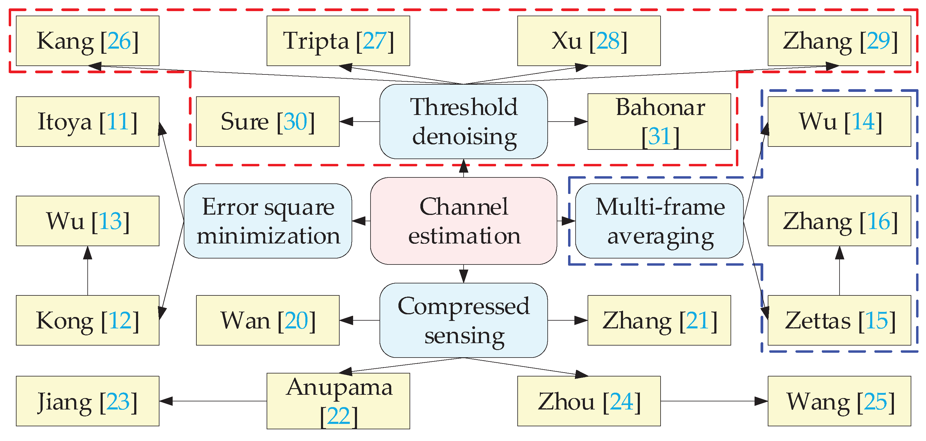
Figure 2.
CP-OFDM system model using the AFS-DT channel estimation method.
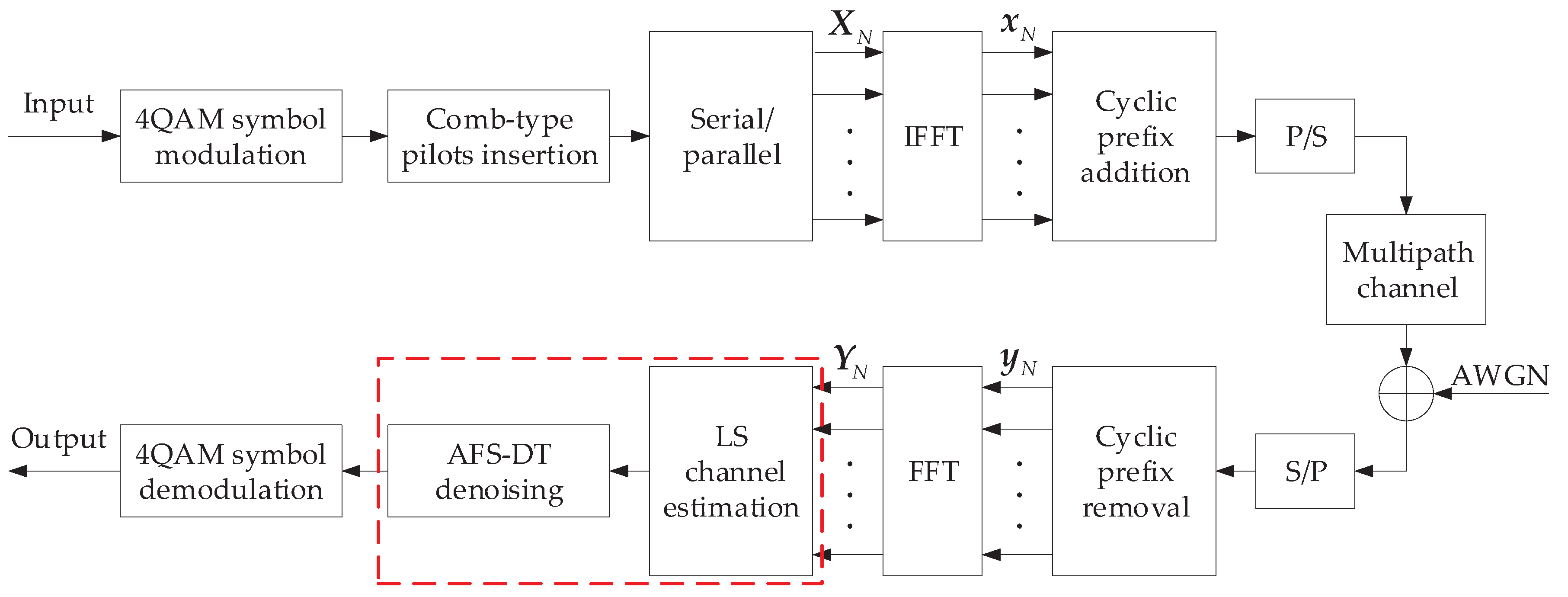
Figure 3.
NMSE of different values: (a) VU and (b) MR.
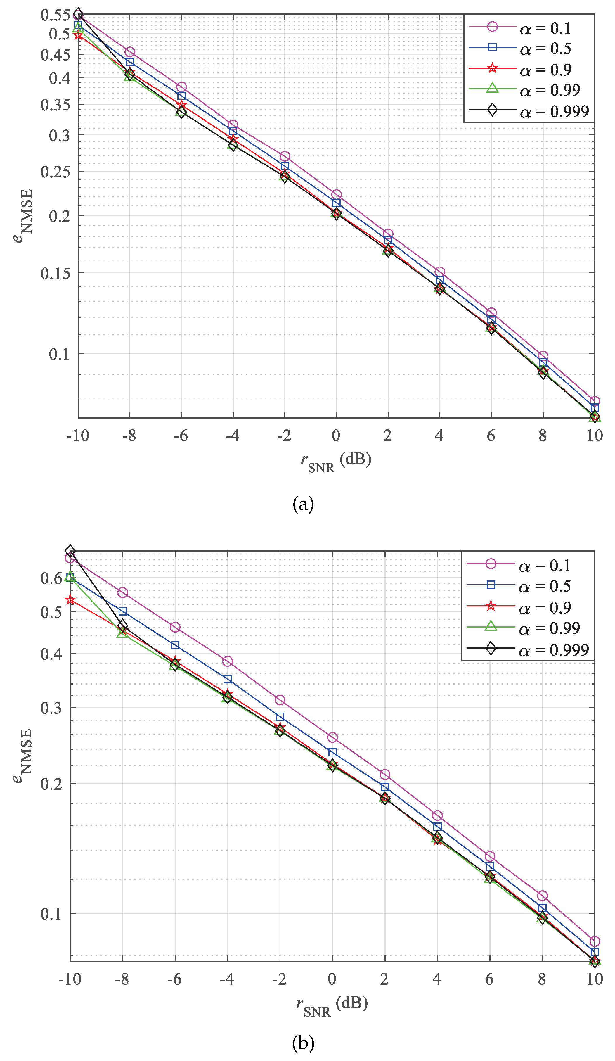
Figure 4.
The performance of different channel estimation methods in VU channel with UE speed of 40 km/h: (a) NMSE and (b) SCDR.
Figure 4.
The performance of different channel estimation methods in VU channel with UE speed of 40 km/h: (a) NMSE and (b) SCDR.
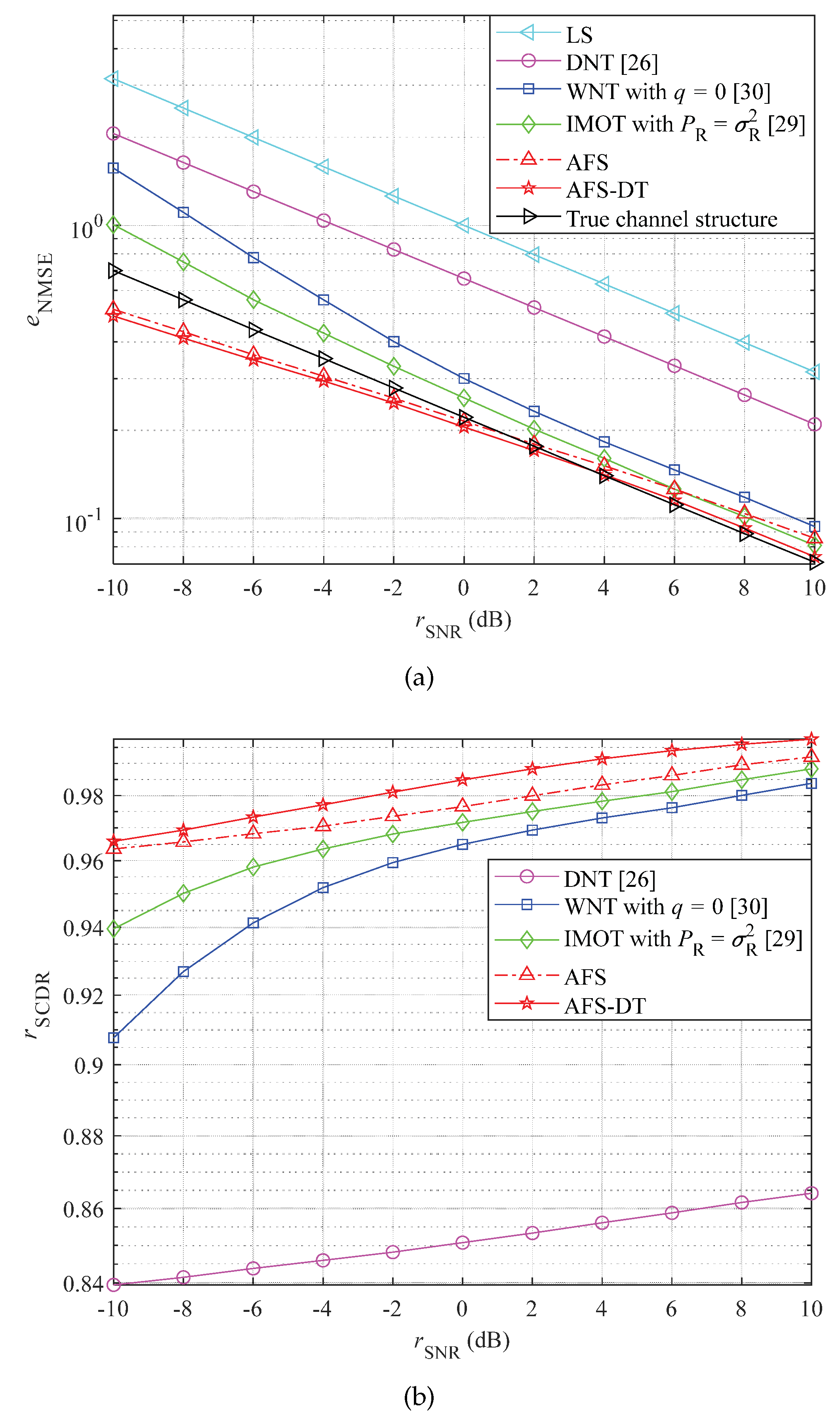
Figure 5.
The performance of different channel estimation methods in MR channel with UE speed of 100 km/h: (a) NMSE and (b) SCDR.
Figure 5.
The performance of different channel estimation methods in MR channel with UE speed of 100 km/h: (a) NMSE and (b) SCDR.
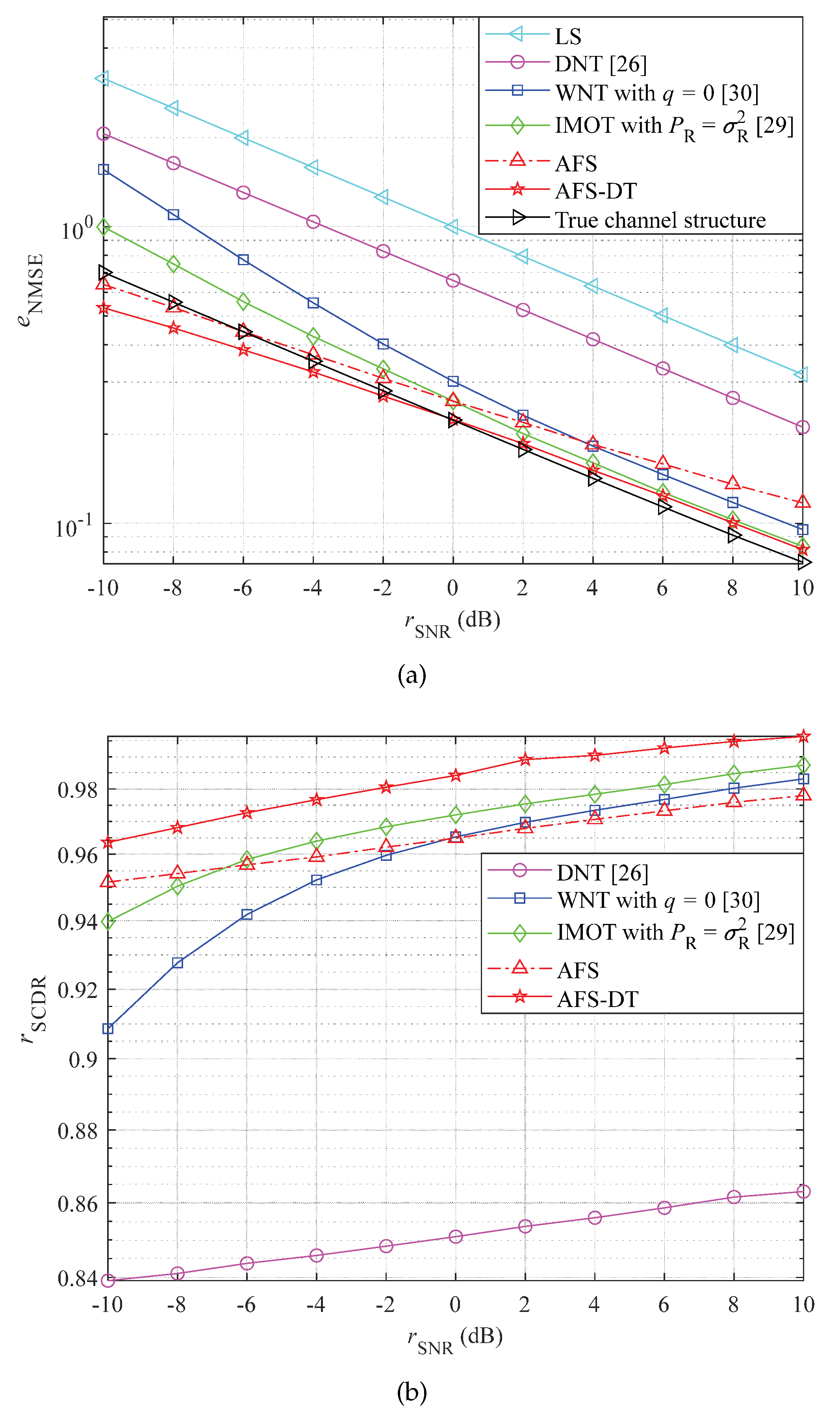
Figure 6.
BER of different channel estimation methods in VU channel with UE speed of 40 km/h.
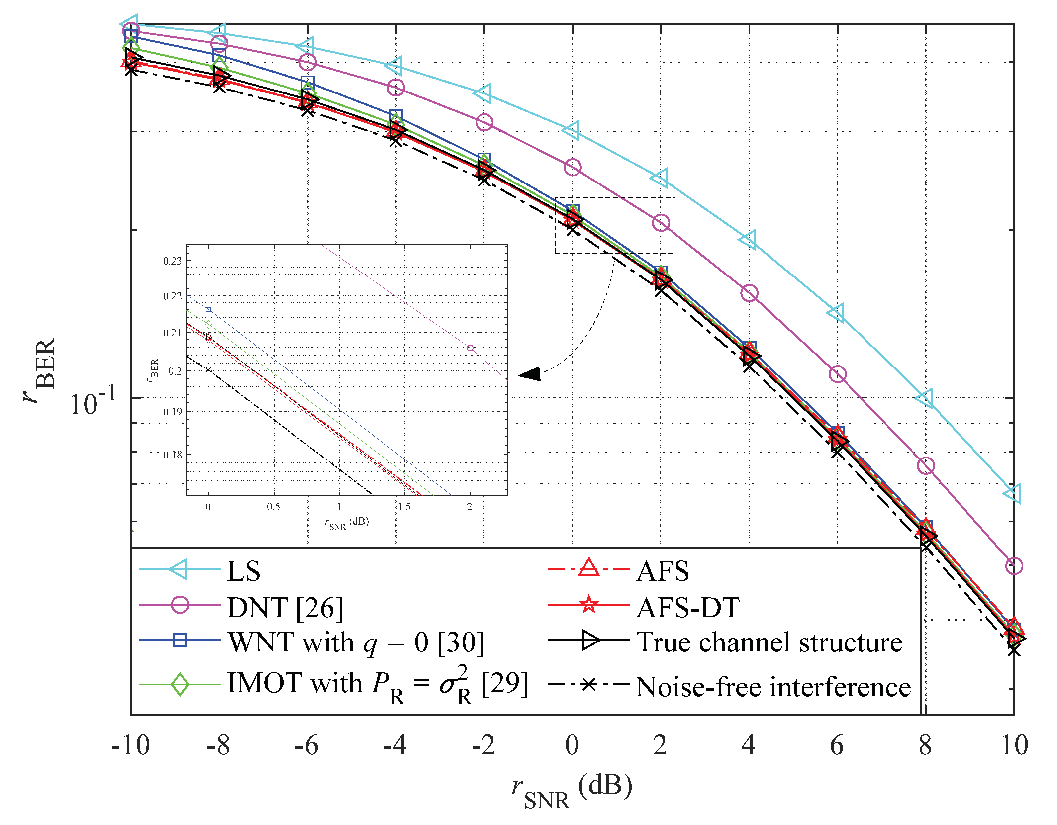
Figure 7.
BER of different channel estimation methods in MR channel with UE speed of 100 km/h.
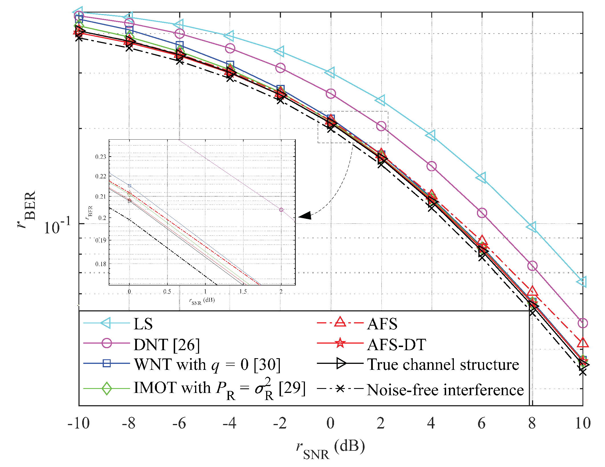

Table 1.
PDP for VU and MR multipath fading channels.
| Tap | VU | MR | ||
|---|---|---|---|---|
| Delay () | Power (dB) | Delay () | Power (dB) | |
| 1 | 0.0 | 0.0 | 0.0 | 0.0 |
| 2 | 0.3 | −0.5 | 0.5 | −1.3 |
| 3 | 0.8 | −1.0 | 1.0 | −3.4 |
| 4 | 1.6 | −4.1 | 1.8 | −6.8 |
| 5 | 2.6 | −8.8 | 2.5 | −10.2 |
| 6 | 3.3 | −12.6 | 3.1 | −12.9 |
| 7 | 4.8 | −18.6 | 3.9 | −16.3 |
| 8 | 5.8 | −21.6 | 4.8 | −19.5 |
| 9 | 7.2 | −24.6 | 5.5 | −21.7 |
| 10 | 10.8 | −20.7 | 6.4 | −23.3 |
| 11 | 11.8 | −18.8 | 7.0 | −24.2 |
| 12 | 12.6 | −19.5 | 9.0 | −25.8 |
Table 2.
Simulation parameters of the OFDM system.
| Parameters | Specifications |
|---|---|
| System model | CP-OFDM |
| Channel distribution | Rayleigh |
| Baseband bandwidth B | 5 MHz |
| Modulation mode | 4QAM |
| The number of OFDM frame K | 400 |
| Subcarrier number (without CP) N | 960 |
| CP length | 240 |
| Pilot interval | 3 |
Disclaimer/Publisher’s Note: The statements, opinions and data contained in all publications are solely those of the individual author(s) and contributor(s) and not of MDPI and/or the editor(s). MDPI and/or the editor(s) disclaim responsibility for any injury to people or property resulting from any ideas, methods, instructions or products referred to in the content. |
© 2023 by the authors. Licensee MDPI, Basel, Switzerland. This article is an open access article distributed under the terms and conditions of the Creative Commons Attribution (CC BY) license (http://creativecommons.org/licenses/by/4.0/).
Copyright: This open access article is published under a Creative Commons CC BY 4.0 license, which permit the free download, distribution, and reuse, provided that the author and preprint are cited in any reuse.


