Submitted:
06 June 2023
Posted:
07 June 2023
You are already at the latest version
Abstract
Within this paper, a machine learning algorithm is used to investigate the importance of certain setpoints and parameters in the filtration processes of a large-scale water treatment facility. Previously, a model for the filtration process based on Run-to-Run Control was proposed and tested against sample data from the treatment plant, but it was quickly found that such a model was incompatible for successfully computing setpoints of operation which minimize the energy cost of running the filtration systems. The machine learning model described herein is an attempt to elucidate the importance of the available data on the filtration systems and to identify the most important variables that influence the filtration run time.
Keywords:
Filtration
; Water Treatment
; Water Management
; Machine Learning
; Run-to-Run Control
1. Introduction
Filtration technologies on large-scale systems are very useful for a wide variety of applications. In particular for water treatment plants, filtration is a key component of the treatment process. Unfortunately, the flows inside filtration processes for large-scale systems are often complicated due to membrane fouling, a process in which excess permeate from the fluid flows builds up on the filtration layers over time, causing a significant decrease in filtration efficiency [4]. In practice, this is usually countered by employing backwashing, in which the flow through the filtration layers is reversed to blow out any built up permeate [2]. This can create turbulent flows, and depending on the filtration/backwashing schedule given, this often prevents a given filtration system from reaching a steady flow state. As a result, it is very difficult to capture the dynamics of a filtration system entirely. The situation is further complicated as many different filtration systems used in industrial applications do not have many useful measurements of quantities that would allow such a model to be developed [1]. Nevertheless, many attempts have been made throughout the body of research to formulate models of filtration which not only capture this chaotic behavior inside filtration systems, but also uses this knowledge to inform the system operators of how to adjust setpoints of operation for future filtration cycles to reduce plant operation cost.
One such model that attempts to perform this task is the Run-to-Run Control model for filtration. Run-to-Run Control is a general process model that was initially considered for semi-conductor manufacturing processes in which silicon wafers are created in batches [5], and has since been used as a successful controlling strategy in a variety of applications, ranging from the control of batch chromatography [10], yeast fermentation [11], and batch polymerization [12].
The purpose of a Run-to-Run Controller is to calculate operating setpoints in between the periodic cycles or batches of the given process. Once calculated, standard PID-type controllers (Proportional, integral, and derivative) are employed to realize these setpoints during the next cycle or batch. The Run-to-Run controller itself is not a PID-controller, since it is active only in between batches. The calculation of these setpoints is based on a very simple process model that is updated using data gathered from the previous batch. Run-to-Run Controllers update the model itself to adapt to any changes that occur in the system over countless cycles. This is especially useful for water treatment filtration processes, since over time the running of filtration/backwashing cycles affects the permeability of the filtration layers, which in turn will affect the underlying physical parameters that govern the modeling of the resistance of these layers.
The idea of a general Run-to-Run Controller is illustrated in Figure 1. Here, u represents the control setpoints for the independent variables that are computed by the Run-to-Run Controller, v represents the outputs from the base controller, y represents the measurements taken from the process, p represents the parameters and initial states of the process, and is the objective function for the control problem. A thorough literature review on Run-to-Run Control processes is given in [13].
Such a model is described in detail in [1,2,3], and has been applied to a test water treatment facility in [6] to determine if it was feasible for larger scale filtration systems. This particular facility is composed of 20 deep bed, dual media gravity filters. These filters are all rectangular basins, 22 ft. wide by 44 ft. long, organized into two rows of 10 filters each. Influent flow is split into two channels and fed to each set of 10 filters through six trough openings installed in each filter half. For each half, there a nine filters which use a 72 inch layer of anthracite coal followed by an eight inch layer of sand for the filter medium, and one filter which uses a 72 inch layer of granulated activated carbon followed by an eight inch layer of sand for the filter medium. It should also be noted that the raw water quality of the inflows into the filters is very high, with a mean maximum turbidity averaging around 0.19 NTU.
The aforementioned model for the filtration cycles describes the dynamics of full filtration/backwashing cycles for one of these filter basins. The model updates the physical parameters which describe the current state of the filtration media in between cycles, and computes ideal setpoints of operation for future filtration cycles to minimize cost of operation.
After several experiments, it was concluded that the Run-to-Run Control model, while successful on smaller scale filtration systems, was insufficient to describe the dynamics for the larger scale water treatment plant [6]. Because of this failing, it is now important to understand the relationships between the available treatment plant data and the desired outputs of the system in order to understand how to modify and correct this model. To this end, a machine learning algorithm will be developed in this paper to undertake this task.
Machine learning at its core is a method of using computer algorithms which allow one to predict how inputs of a particular model or system affect the outputs of that system. In this case, it was decided to use algorithms to create regression decision trees on how to predict filtration times. There are many sources on the theory behind constructing these types of decision tree algorithms, such as in [15,16]. Regression tree models "learn" about the nature between the input variables and output variables of a given process by observing many different cases of these variables being related to each other. This large set of input and output variables is called the training data for the model. The more training data that is utilized, the better the model is able to classify certain types of input which give rise to desired outputs.
In the case of regression tree models, the algorithm begins by looking at all the training data and splitting the data into two sets with two different output predictions based on the magnitude of the input. The input and threshold value are chosen to minimize the error in output prediction in the two categories. From here, the algorithm recursively splits the two sets even further using other input variables to determine the parsing of the training data, with the goal of minimizing prediction error at each step. The splitting of the data stops once a sufficient error in prediction is achieved on the training data. At the end, a tree is formed which predicts the output of a given sample of input data by following the splits in the tree based on the values of the input data at each split [15].
In these decision trees, the input variables which are chosen to split the data are deemed to have more importance in predicting the output. The higher these variables appear on the tree, and the more often they appear through the decision process, the more importance they have to the overall prediction. By investigating these tree models, one can gain a sense of which input variables are useful in predicting an overall run time for the filtration process. Moreover, by creating decision trees on subsets of the training data that have more similarity, such as filtration cycles which occur in the same season, the importance of the input variables in predicting run times can be assessed for cycles appearing in these specific subsets.
Machine learning and artificial intelligence have taken on a plethora of applications in recent years, and applications for water filtration systems of all kinds are no exception. Recent applications of machine learning and AI to water treatment processes systems are summarized in [7,8,9]. To the author’s knowledge, there have been no studies conducted on the application of regression tree models to the determination of filtration run time for large scale filtration systems in a water treatment plant.
In the second section of this paper, the formulation of this machine learning model is presented, the available measured inputs from the test water treatment plant are given, and the preparation of this data for the machine learning model is explained. In the third section of this paper, the implementation of this model is outlined, and the results of running this model on the prepared data are presented. In the final section of the paper, some conclusions are drawn from the outcomes of the experiments, and future directions for this work are presented.
2. Materials and Methods
For the filtration systems at the test water treatment plant, the most important measured quantities for water quality have been selected to analyze their predictor importance in determining the setpoints of operation for a given filtration/backwashing cycle. There are several different quantities that are measurable from this water treatment plant, however, the only ones that were considered were quantities that were either directly related to the Run-to-Run Control model variables in some way, or were direct inputs to the filtration systems themselves. In total, there are 11 different measured variables that are used in this machine learning model.
First, there is the effluent flow into the filtration tanks itself. The treatment plant tracks several quantities pertaining to this flow which are taken as inputs for the machine learning model. The flow rate is measured hourly, and over each cycle, the mean flow rate and mean flow temperature are calculated and taken as two separate input variables for the model. In addition, for each cycle, the difference between the highest flow rate and the lowest flow rate, i.e. the flow spread is also calculated and taken as an input variable.
The next two variables considered are turbidity measurements of the influent flow into the filtration tanks and the effluent flow out of the filtration tanks. These quantities are of special interest mainly because they are a primary indicator of overall water quality, but also because they are directly correlated with the viscosity of the filter feed, which is a key variable used in the Run-to-Run Control model. The turbidity is measured hourly for both influent and effluent flows, and for each cycle, the mean turbidity of the influent and effluent flows during filtration are both calculated and used as input variables.
Another important feature of the filtration process is headloss, a quantity that measures the loss of pressure in the fluid flow from the start of filtration to the end of filtration. This quantity is directly correlated to the transmembrane pressure (TMP) across the filtration layers, which is the most important quantity of interest in the Run-to-Run Control model. To capture the overall contribution of headloss to filtration run times, it is analyzed in the following manner. It is observed from treatment plant data that the headloss during any filtration cycle generally increases linearly over time. Hence, to capture this linear behavior, for each cycle, a linear polynomial is fit to the headloss data that is measured hourly for each cycle. From this linear fit, the slope of the line, which is named headloss slope, and the intercept of this line, which is named headloss intercept, are computed. These give the average rate of increase in headloss over the entire cycle, and the headloss at the beginning of each cycle, respectively, and both are taken as input variables for the machine learning model.
One very important feature from the perspective of operational costs is the power usage during filtration. By gauging the importance of power usage to the overall runtime of filtration, it is then possible to better understand how control strategies can be developed to optimize the overall usage and reduce plant operation costs. Hence, power measurements were collected hourly as well, and a mean power usage for each filtration cycle are calculated and used as a predictor in this model.
Finally, measurements from previous components of the water treatment process are also taken as input variables, since they constitute the initial conditions of the feed fluid. In this particular water treatment plant, the filtration systems are fed from two different sources; the ozonation tanks and the flocculation tanks. Ozonation tanks add ozone to the fluid feed to oxidize different particulates in the water to insoluble compounds which are easier to filter out, thus effectively acting as a disinfectant. Flocculation tanks encourage the aggregation of small suspended particles in the water into much larger clumps, making it much easier for them to settle out during the filtration process. From each of these sources, there are measured quantities that influence the overall water quality going in, and hence should influence the overall filtration time as well. These quantities are the turbidity of the ozonation flow, the pH of the flocculation water flow, and the particle count of the flocculation flow. For each of these variables, hourly measurements are taken over each filtration cycle, and the means of these three variables are taken as input for the machine learning model.
In total, the raw training data for this machine learning model consists of 247 separate filtration cycles spanning seven years of plant operation, from the beginning of 2016 to the end of 2022. Filtration run times for each cycle are on average about 202 hours, with a minimum run time of 77 hours and a maximum run time of 552 hours. In general, most filtration cycles aim optimally for around 170 to 200 hours of runtime, but some cycles deviate from this norm due to different filtering conditions. In particular, the largest filtration runtime anomaly from this dataset was a period from August, 2021 to February, 2022 in which run times over 10 cycles ranged from 280 hours up to 550 hours. This was attributed to a stuck influent valve to the filtration unit, which drastically reduced influent flows, resulting in longer run times due to not having to backwash as often. In order to achieve a model that gives optimal for the typical filtration run times, cycles with outlier run times are removed from the training set at the start. In total, 17 cycles were removed from the dataset, leaving 230 cycles to be used as training data for the model.
This data has also been collected and parsed into separate sets for each season the cycles were run under. In total, there are 45 winter cycles, 51 spring cycles, 74 summer cycles, and 60 fall cycles. Moreover, the filtration system has two modes of pumping influent flows into the filtration units, namely flat pumping and bathtub pumping. The filtration systems were mostly run under flat pumping during these seven years, however bathtub pumping was implemented during the periods of May 24th, 2021 to November 1st, 2021 and May 30th, 2022 to October 1st, 2022. Since these periods primarily affected the summer cycles, the summer filtration data was parsed into two separate subsets for cycles under flat pumping versus cycles under bathtub pumping. In total, there were 57 cycles for the Summer flat pumping set, and 17 cycles for the Summer bathtub pumping set.
In addition to training this model over the full seven years, the model was also trained specifically for each season, as well as specifically for each mode of pumping during the Summer. The idea was to see if any specific trends during these time periods were present, and if different seasons and pumping strategies favored different quantities of interest. As will be seen in the results section, this turns out to be the case.
In order to implement this machine learning model, a script was written to compute a regression tree and predictor importance for the eleven input variables using the fitrtree algorithm in MATLAB. In addition, the creation of regression tree ensembles to quantify out of bag error was implemented in this script using the TreeBagger algorithm in MATLAB. Details about the implementations and algorithms behind these two MATLAB functions can be found here [18,19].
3. Results
Seven different experiments were performed according to seven different training data subsets, namely the winter, spring, summer, fall, all seasons, summer flat pumping, and summer bath pumping subsets described in the previous section.
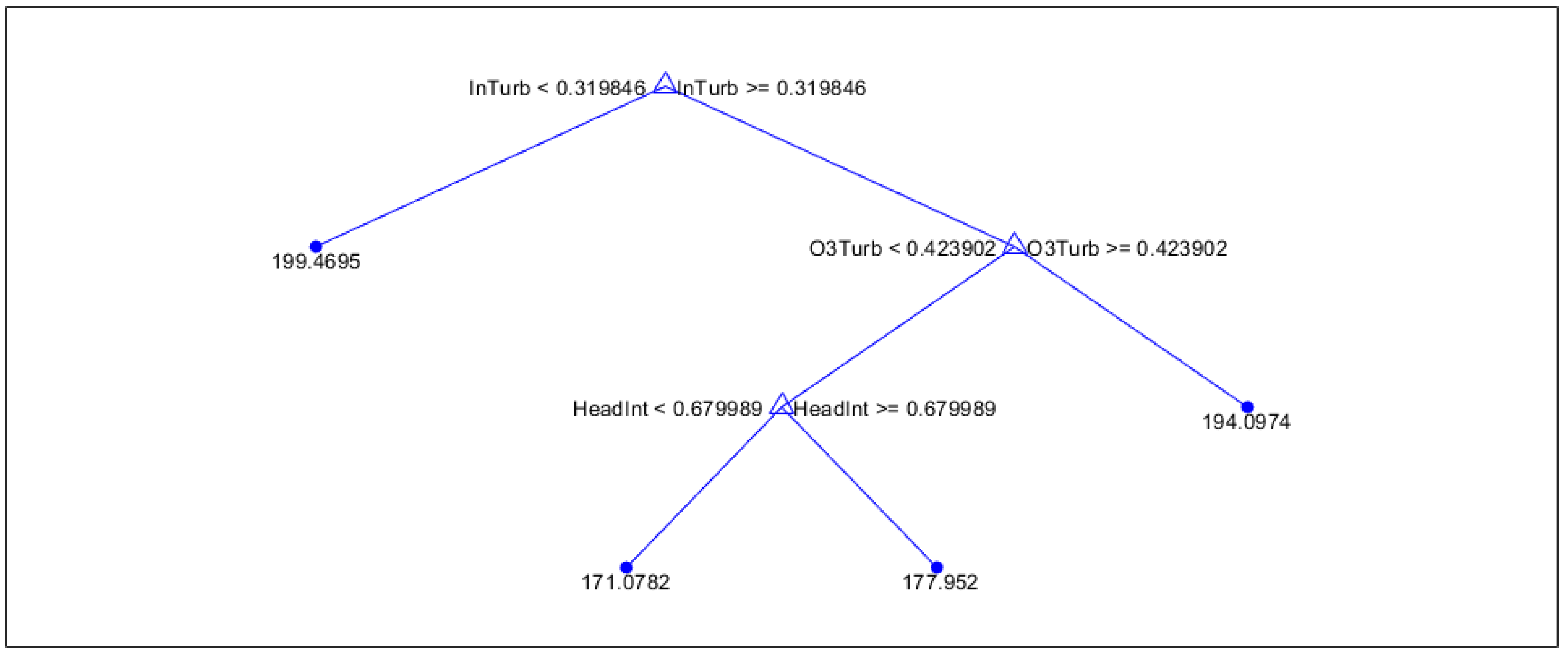
To implement experiments using fitrtree, the optimal number of splits in the decision tree was first calculated for each experiment. To do this, the algorithm was run on all predictor variables while letting the maximum number of splits made in the trees vary from two splits all the way up to 50 splits. For each of these experiments, the resubstitution losses and cross validation losses were tracked and compared. For all seven training subsets, it was found that the cross validation error fluctuates erratically as the number of splits increases up to 50, but generally stays within a specific range. Because of this random fluctuation, the cross validation error is not considered for selecting the optimal maximum number of splits. Instead, the resubstitution error is used, which was found to decrease as the number of splits increases for all seven training subsets. The plot of the resubstitution errors over the maximum number of splits allowed is shown in Figure 2. For each training subset, the number of splits for the decision tree were then chosen corresponding to the point where the resubstitution error levels out and starts decreasing very little or not at all in certain cases. The decision trees with these optimal number of splits are shown in Figure 3, Figure 4 and Figure 5 and in the appendix in Figure A1–Figure A4.
For each of these decision trees, a cross validation error is calculated by passing the decision tree through cvloss function 100 times, and taking the mean of all the results obtained. This gives a nice representation of how well the decision tree performs in predicting for data samples outside the training set. This cross validation loss, and the resubstitution loss for each decision tree are reported in Table 1. The results show that the decision trees generally fit their training sets fairly well, but predict new training samples with less accuracy. For example, in Table 1 Winter predicts within its training set with an expected error of 5.41 hours, while for new data the error is expected to be about 13.91 hours, and since the range of filtration times given for this particular training set was 54 hours, the error in prediction is about a quarter of the size of the range of filtration run times expected to be observed.
From the decision trees in Figure 3, Figure 4 and Figure 5 and Figure A1–Figure A4, the most important predictors the model used to predict runtimes are seen in first two splits. For winter, the two most important predictors were flocculation PC and flocculation pH, showing that conditions of the influent from the flocculation tanks are good indicators of run times. For the spring, flocculation PC and the effluent flow spread are the two most important predictors, showing that the range of flows entering the filtration unit has a decent contribution to the overall runtime. For summer, the turbidity of the effluent flow out of the filtration tanks is the primary predictor, with headloss slope and water temperature playing a secondary role. This shows that the water quality exiting filtration is a good predictor of runtime in this season. In the fall, the power usage and filter temperature are the most important indicators of filtration run time, indicating that power usage is especially important in the fall.
In general, for all seasons, power usage is a primary indicator, while flocculation PC and effluent turbidity are important secondary indicators. Lower power usage will mostly lead to longer filtration times, and in this case the time depends on the flocculation PC, water temperature, and effluent turbidity. For the shorter filtration times, the exact prediction, then depends on effluent turbidity, power usages, and water temperature.
Finally, when investigating the two pumping strategies used during the summer, it can be seen that for flat pumping cycles, effluent turbidity is the primary indicator, while flocculation PC and pH are both secondary indicators. In the case of bath pumping, the primary two indicators are influent turbidity and turbidity.
In an effort to improve the prediction quality of this model for cycles outside the training set, an algorithm employing treebagger was used to create bagged tree ensembles with 100 trees each. For each training subset, the maximum number of splits used to determine the trees in the previous experiments were used. To gauge the accuracy in prediction of these ensembles, the average, minimum, and maximum out of bag errors were calculated for each ensemble, and the results are shown in Table 2. It is easy to see that the out of bag error averages are all less than the cross validation losses in the previous experiments, which shows that the tree ensembles have better quality predicting power than the decision trees produced by fitrtree. Moreover, the average out of bag error is very close to the minimum out of bag error in each ensemble, showing that the ensemble reaches a steady error in prediction very quickly.
4. Discussion
Overall, the results of these experiments seem to indicate that the seasonal patterns of weather in the region have a high influence in what quantities measured at the water treatment plant are good predictors of the final run time of any given filtration cycle. In particular, during the winter and the spring, contributions from the flocculation tanks play a major role in determining run times, while water temperature and turbidity of the flows coming in and out are useful for the summer and fall. Moreover, a general predictor that works well for all seasons is usage of power, which can determine roughly if the current cycle will be a shorter or longer one.
The summer seasonal experiments also show that different types of pumping strategies for filtration have an effect on what quantities are most important to monitor. When utilizing bathtub pumping, it is most important to monitor the turbidity of the influent and the turbidity of water flowing in from the ozonation tanks. In contrast, while using the flat pumping strategy, the effluent turbidity from filtration and water quality coming in from the flocculation tanks plays a more prominent role instead. When considering all cycles during the summer, the model mainly identified the effluent turbidity as an important factor, but by parsing the data into two separate bins for the different pumping strategies, it reveals which contributors to overall turbidity are most important in determining the overall runtime. This again emphasizes the importance of separating cycles with different pumping strategies.
The importance of turbidity in the summer could most likely be explained by the increased demand for water in Las Vegas during these months. This leads to an increased inflow into Lake Mead from the Vegas Valley Wash, which in turn can affect the raw water quality accepted into the intakes. In particular, the turbidity of the water along the wash is much higher during the summer. Moreover, there has been a substantial decrease in the lake volume of Lake Mead over recent years. These two factors cause more recycled water to be present at the intake, which likely drives the general preference of the model to turbidity. When utilizing bathtub pumping, it can be seen that the lower the influent turbidity and turbidity are, the quicker the run times tend to be. On the other hand, when using flat pumping, lower pH and particle counts in the flow from the flocculation tanks will also lead to lower filtration run times.
One possible cause for the model’s preference to headloss slope and flocculation particle counts in the Spring could be due to the annual process of destratification in Lake Mead, which is the source of the inflow to the treatment plant. Lake turnover for Lake Mead typically begins in November, and the destratification of the thermal layers is mostly complete by February, but it is noted in [17] that Lake Mead doesn’t full destratify every year, which leads to the lake having a partial mixing of the thermal layers during the Spring months before lake stratification normalizes the thermal layers around May or June of each year. During the Spring, the intakes deliver inflows which are of a much different nature than during other times of the year, when the lake exhibits more regularity of water quality at the intakes. Since this data set spans enough time to incorporate several years of complete turnover, lake turnover is likely driving the preference of this model to headloss and flocculation particle counts despite the fact that it does not occur every year.
The fall experiments show a preference to power usage and filtration temperature as primary predictors of runtime, while in the winter the model shows a high preference to flocculation pH and particle counts. The overall picture for all seasons shows a similar preference to power in the fall, and both experiments indicate that smaller mean power consumption in general leads to longer filtration times, while larger mean power consumption in general leads to shorter filtration times. This suggests that the rate of power consumption will not have as much of an effect on overall power used per filtration cycle.
To improve on the results of these models, future work on this project involves analyzing the importance of predictors within the tree ensembles produced by this model and see how they compare to the predictors produced from fitrtree. It is clear that the tree ensembles produce more accurate predictions, but the random nature of their construction coupled with the amount of trees produced makes it difficult to analyze predictor importance. In addition, more research could be conducted using this model with larger training data sets to try and improve the overall accuracy of the fitrtree model. In particular, more summer cycles utilizing bathtub pumping are desperately needed, as this was not used as much during the seven years of data collected to train this model. It would also be advantageous to try and run this model for data sets which are parsed according to differing weather conditions, such as dry weather versus stormy flood weather, to see if not only seasonal predictors are present, but if new predictors arise during certain types of weather periods.
Author Contributions
Conceptualization, Jeffrey Belding and Deena Hannoun; Data curation, Jeffrey Belding; Formal analysis, Jeffrey Belding; Funding acquisition, Deena Hannoun; Investigation, Jeffrey Belding; Methodology, Jeffrey Belding and Deena Hannoun; Project administration, Deena Hannoun; Supervision, Deena Hannoun; Visualization, Jeffrey Belding; Writing – original draft, Jeffrey Belding; Writing – review & editing, Jeffrey Belding and Deena Hannoun.
Funding
The authors would like to thank the United States Bureau of Reclamation WaterSMART Drought 465 Resiliency program [R18AC00021] for providing funding for this project.
Data Availability Statement
The data used in this paper is not publicly available, please contact the corresponding authors with any inquiries.
Acknowledgments
The authors would like to thank Robert Devaney, Todd Tietjen, and Daniel Chan for reviewing this work and offering constructive feedback
Conflicts of Interest
All authors of this article declare no conflicts of interest in conducting this research and experimentation.
Appendix A - Decision Trees
Figure A1.
Fall regression tree
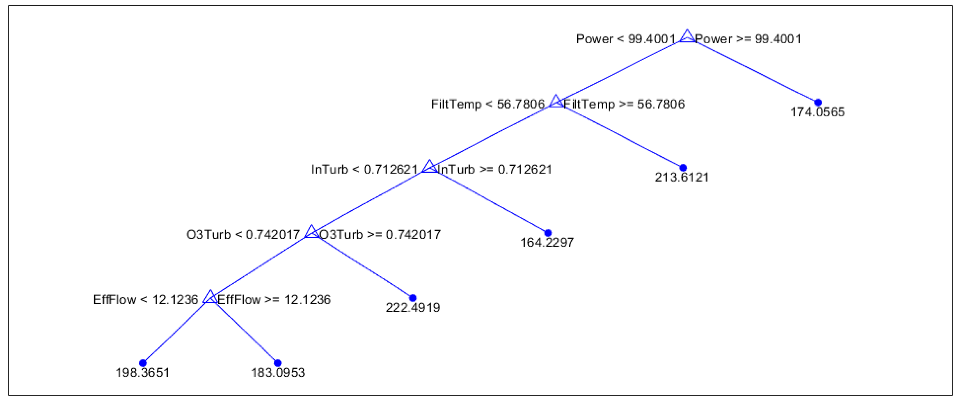
Figure A2.
All seasons regression tree
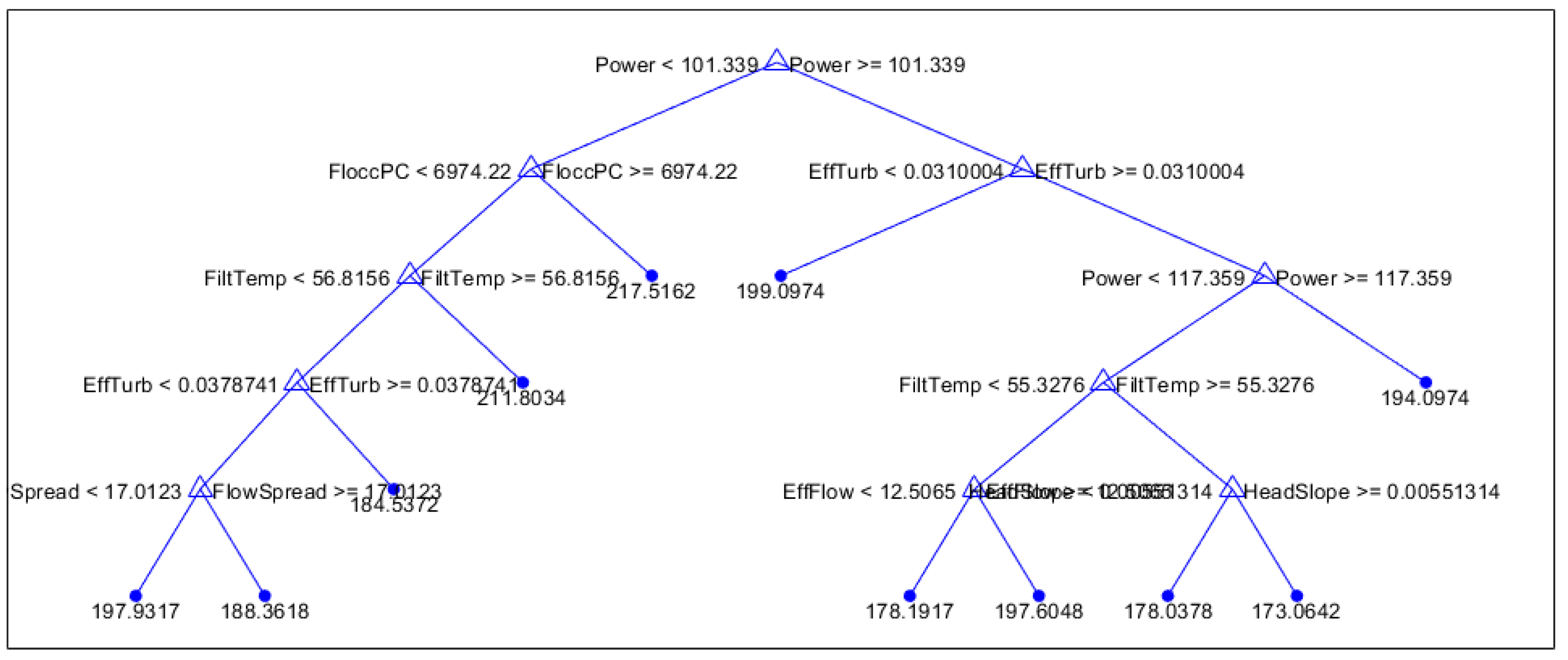
Figure A3.
Summer flat pumping regression tree
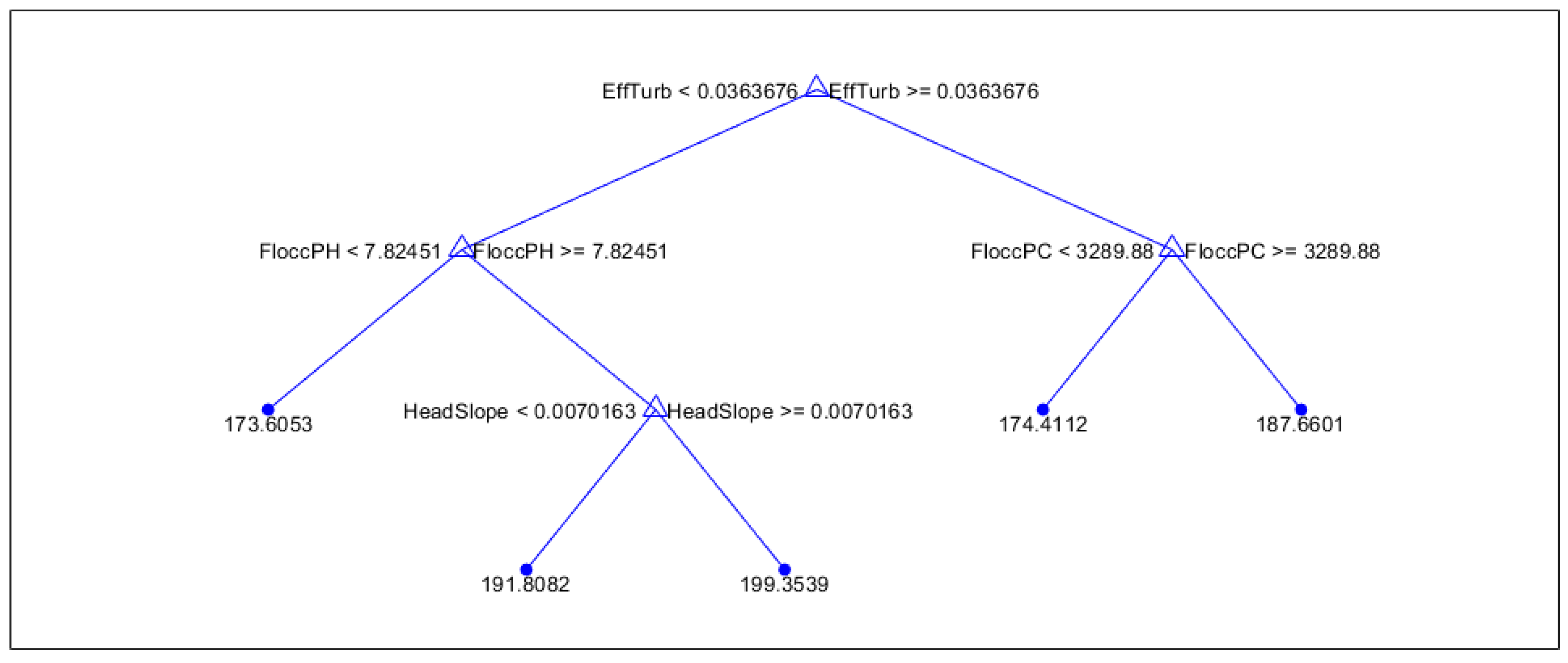
Figure A4.
Summer bath pumping regression tree
References
- Busch, J.; Cruse, A.; Marquardt, W. Run-to-run control of membrane filtration processes, AiChE Journal 2007, 53, 2316-2328.
- Busch, J.; Marquardt, W. Run-to-run control of membrane filtration processes, IFAC Proceedings Volumes, 2006, 39 1003-1008.
- Busch, J.; Marquardt, W. Run-to-run control of membrane filtration in wastewater treatment - an experimental study, IFAC Proceedings, 2007, 40, 195-200.
- Jepsen, K.; Bram, M.; Hansen, L.; Yang, Z.; Lauridsen, S. Online backwash optimization of membrane filtration for produced water treatment, Membranes, 2019, 9, 68.
- Sachs, E.; Hu, A.; Ingolfsson, A.; Langer, P. Modeling and control of an epitaxial silicon deposition process with step disturbances, [1991 Proceedings] IEEE/SEMI Advanced Semiconductor Manufacturing Conference and Workshop, 1991, 104-107.
- J. Belding, Numerical studies of regularized Navier-Stokes equations and an application of a Run-to-Run control model for membrane filtration at a large urban water treatment facility, Doctoral Dissertation, University of Nevada Las Vegas, 4505 S Maryland Pkwy, Las Vegas, NV 89154, 21. 20 December.
- L. Li; S. Rong; R. Wang; S. Yu, Recent advances in artificial intelligence and machine learning for nonlinear relationship analysis and process control in drinking water treatment: A review, Chemical Engineering Journal, 2021, 405, 126673.
- M. Lowe; R. Qin, X. Mao, A review on machine learning, artificial intelligence, and smart technology in water treatment and monitoring, Water, 2022, 14.
- S. Safeer; R. Pandey; B. Rehman; S. Hasan, A review of artificial intelligence in water purification and wastewater treatment: Recent advancements, Journal of Water Process Engineering, 2022, 49, 102974.
- W. Gao; S. Engell, Iterative set-point optimization of batch chromatography, Computers and Chemical Engineering, 2005, 29, 1401-1409.
- D. Bonne; S. Jorgensen, Batch to batch improving control of yeast fermentation. Computer Aided Chemical Engineering, 2001, 9, 621-626.
- Z. Xiong; J. Zhang, A Batch-to-batch iterative optimal control strategy based on recurrent neural network models. Journal of Process Control, 2005, 15, 11-21.
- E. Castillo; A. Hurwitz, Run-to-run process control: Literature review and extensions, Journal of Quality Technology, 1997, 29, 184-196.
- B. Wittenmark, Adaptive dual control methods: An overview. IFAC Proceedings, 1995, 28, 67-72.
- L. Breiman; J. Freidman; C. Stone; R. Olshen, Classification and Regression Trees, Chapman & Hall, 1984.
- J. Brownlee, Master Machine Learning Algorithms, https://machinelearningmastery.com/master-machine-learning-algorithms/.
- J. LaBounty; N. Burns, Characterization of Boulder Basin, Lake Mead, Nevada-Arizona, USA – Based on Analysis of 34 Limnological Parameters, Lake and Reservoir Management, 2005, 29, 277-307.
- "The Mathworks, Inc.", fitrtree, https://www.mathworks.com/help/stats/fitrtree.html, October 26th, 2022.
- "The Mathworks, Inc.", TreeBagger, https://www.mathworks.com/help/stats/treebagger.html, October 26th, 2022.
Figure 1.
Diagram of a generalized run-to-run control process
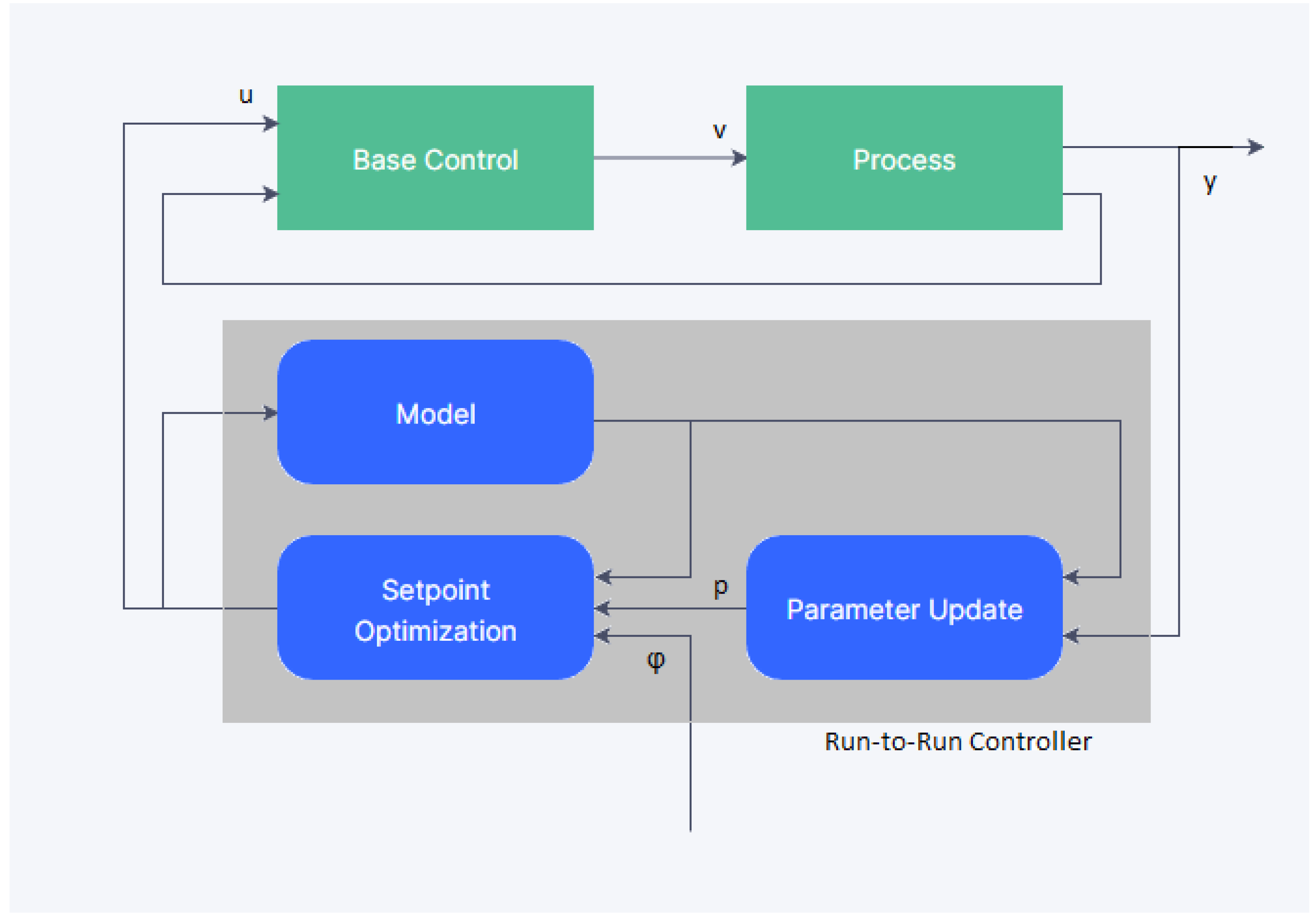
Figure 2.
Graph of resubstitution losses vs. number of splits
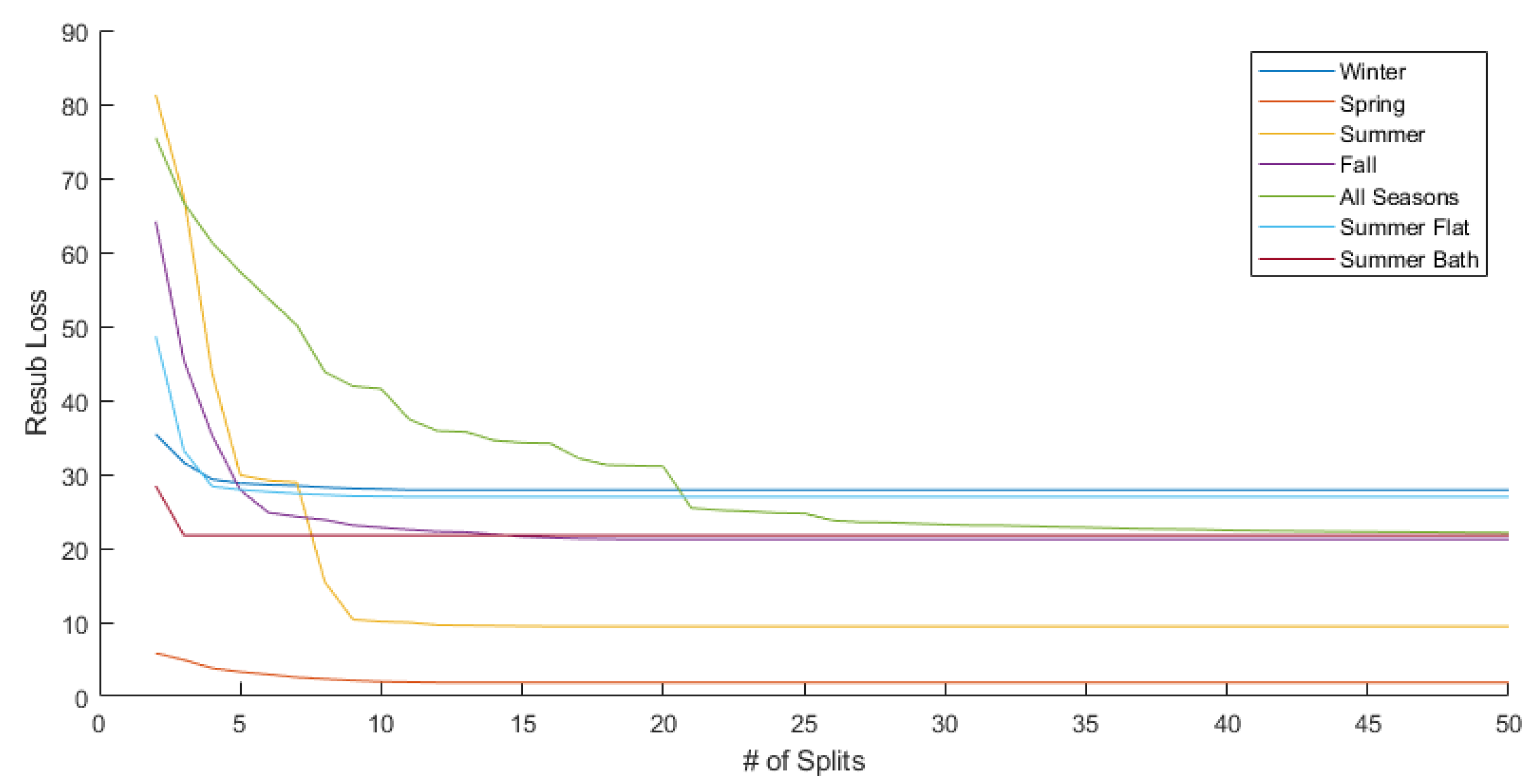
Figure 3.
Winter regression tree
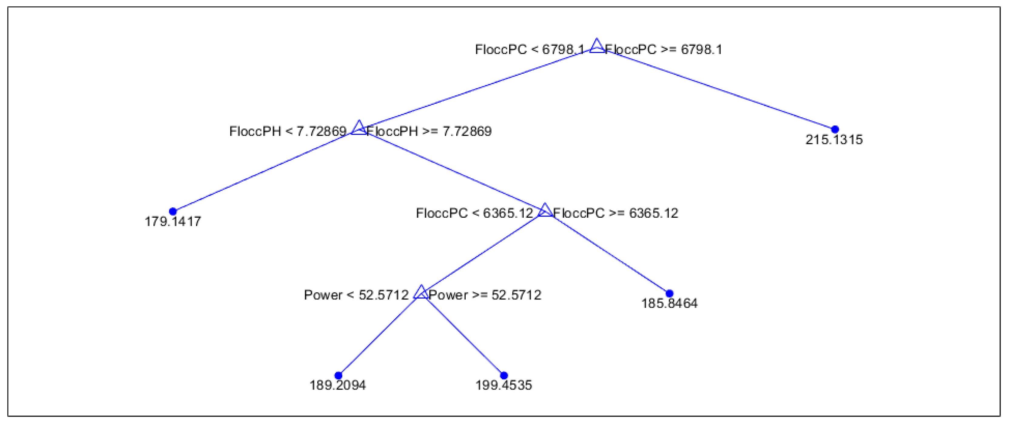
Figure 4.
Spring regression tree
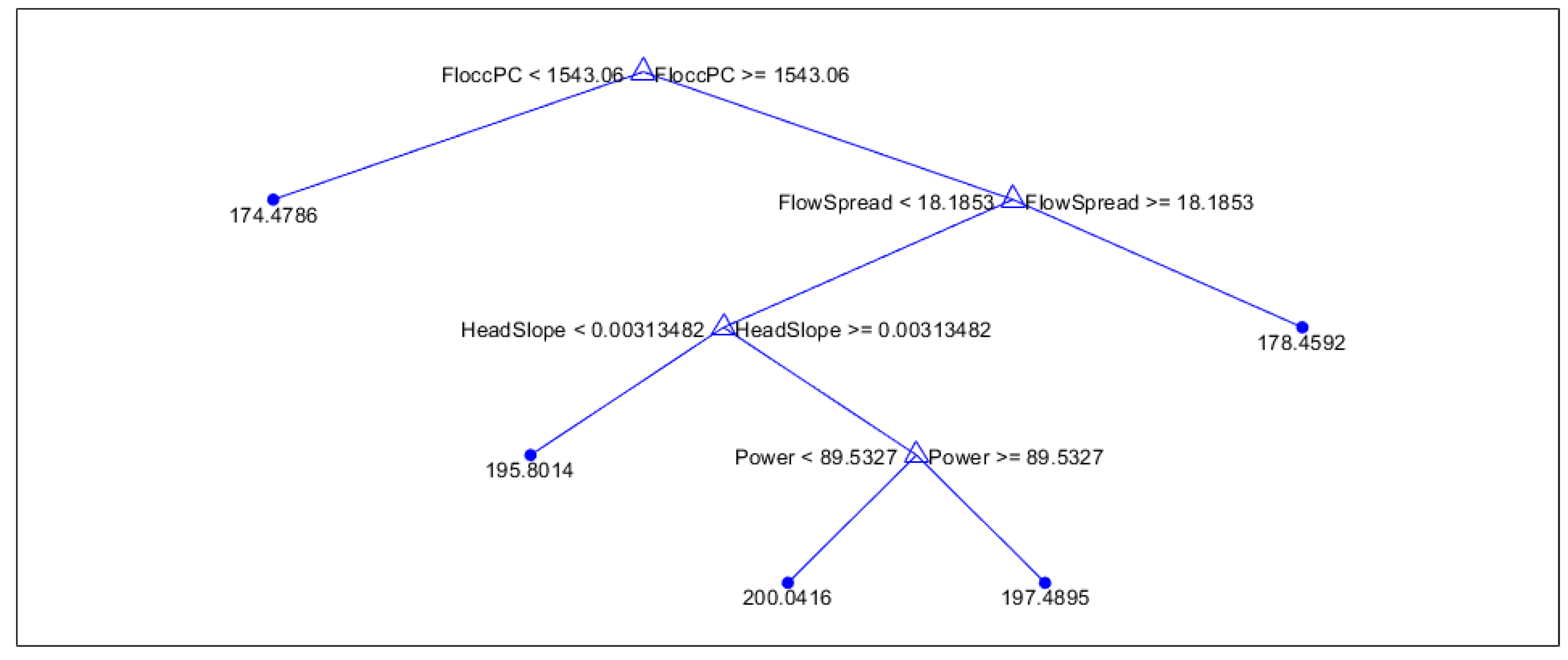
Figure 5.
Summer regression tree
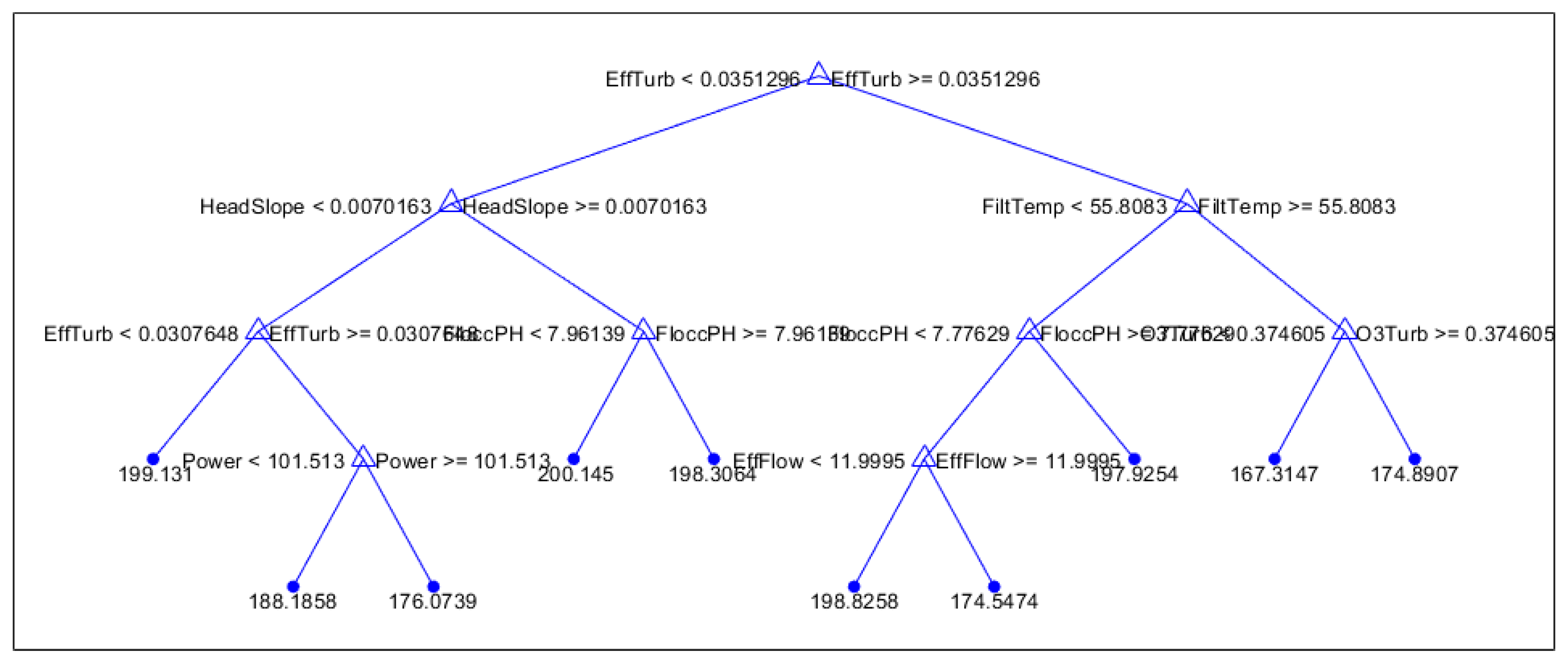

Table 1.
Resubstitution loss and cross validation loss from fitrtree using all categorical predictors.
Table 1.
Resubstitution loss and cross validation loss from fitrtree using all categorical predictors.
| Seasonal Run | Resub. Loss | CV Loss | Run Time Range |
|---|---|---|---|
| Winter | 5.41 hrs | 13.91 hrs | 54 hrs |
| Spring | 1.96 hrs | 6.14 hrs | 31 hrs |
| Summer | 3.22 hrs | 11.77 hrs | 36 hrs |
| Fall | 5.28 hrs | 12.42 hrs | 60 hrs |
| All Seasons | 6.45 hrs | 9.69 hrs | 68 hrs |
| Summer Flat | 5.33 hrs | 8.95 hrs | 32 hrs |
| Summer Bath | 4.66 hrs | 14.70 hrs | 33 hrs |
Table 2.
Out of bag errors from treebagger using all categorical predictors
| Seasonal Run | OOB Average | OOB Min | OOB Max |
|---|---|---|---|
| Winter | 9.08 hrs | 8.74 hrs | 10.90 hrs |
| Spring | 4.82 hrs | 4.59 hrs | 5.34 hrs |
| Summer | 9.45 hrs | 8.95 hrs | 12.00 hrs |
| Fall | 10.86 hrs | 10.29 hrs | 14.28 hrs |
| All Seasons | 8.59 hrs | 8.20 hrs | 11.00 hrs |
| Summer Flat | 7.88 hrs | 7.58 hrs | 11.18 hrs |
| Summer Bath | 11.24 hrs | 9.89 hrs | 12.18 hrs |
Disclaimer/Publisher’s Note: The statements, opinions and data contained in all publications are solely those of the individual author(s) and contributor(s) and not of MDPI and/or the editor(s). MDPI and/or the editor(s) disclaim responsibility for any injury to people or property resulting from any ideas, methods, instructions or products referred to in the content. |
© 2023 by the authors. Licensee MDPI, Basel, Switzerland. This article is an open access article distributed under the terms and conditions of the Creative Commons Attribution (CC BY) license (http://creativecommons.org/licenses/by/4.0/).
Copyright: This open access article is published under a Creative Commons CC BY 4.0 license, which permit the free download, distribution, and reuse, provided that the author and preprint are cited in any reuse.


