Submitted:
01 June 2023
Posted:
02 June 2023
Read the latest preprint version here
Abstract
The present investigation focuses on the impact of jet nozzle installation positions on mixing time in a cylindrical tank. The aim is to identify nozzle positions that achieve maximum mixing efficiency and to elucidate the governing parameters that enhance jet mixing performance. A water tank was employed for the experiment. The jet nozzle vertical inclination angle (α) and the horizontal inclination (β) determined the nozzle positions. Mixing time was determined by a tracer study, utilising a spectrophotometry approach. The findings suggest that the mixing time is significantly influenced by the jet nozzle positions and the extent of the swirling flow resulting from the horizontal placement of the jet nozzle. Regardless of the vertical inclination of the tangentially oriented nozzles, the mixing time increases with the frequency of the bulk fluid swirling flow, even when the free jet path length remains constant. The accuracy of existing models to predict mixing time was evaluated for both conventional centrally aligned (β = 0°) and newly investigated swirling flow-dominated configurations involving tangentially installed nozzles (β > 0°). Our results indicate that the turbulence jet and the circulation model provide accurate predictions for the conventional centrally aligned (β = 0°), upward-pointing jet nozzle installations. For the newly explored swirling flow-dominated configurations involving tangentially installed nozzles (β > 0°) at varying α, we present novel values for the constants of proportionality for both the turbulence jet model and the circulation model, which account for differences in mixing time. Other models largely exhibited either underestimation or overestimation of experimental data for both extreme nozzle installation positions.
Keywords:
Jet mixing
; Mixing
; Mixing time
; Circulation time
; Jet
1. Introduction
Jet mixing is a widely used process that utilises kinetic energy from a pumped stream to blend miscible fluids in tanks or reactors [1,2]. It is particularly effective for large storage tanks where mechanical agitation is impossible to implement [3,4]. The process entails the high-speed recirculation of tank fluid in the form of a jet stream, which is directed through a nozzle and reintroduced into the bulk fluid of the tank. The jet stream is subjected to progressive characteristics modifications across the shear layer, starting from the nozzle inlet and the entire downstream sections. Laboratory observations reveal that fluid jets entering ambient fluid consistently adopt an approximately conical shape with a universal opening angle of 11.80°, regardless of the fluid type, nozzle diameter, and injection speed [5]. The shear flow between a turbulent jet fluid and the surrounding ambient fluid can be divided into three regions [5,6]: the initial region, consisting of a potential core, a small conical-shaped core formed by mixing the jet and ambient fluid. The potential core possesses the flow characteristics of the nozzle inlet and spans a length of approximately six times the diameter of the jet nozzle, dj; the transition region occurs where vortex cores form due to shear flow, subsequently combining to generate larger eddies that break down into smaller ones downstream. This process facilitates mixing and entrainment of the ambient fluid, commencing at approximately eight times the nozzle diameter along the jet axis. Lastly, the fully-developed region is characterised by similarity laws for mean velocity, spread angle, and entrainment. The fully-developed zone to typically commences at 30dj, along the jet axis [5,27].
The velocity of fluid at the centreline of a turbulent jet reduces as it moves downstream due to mixing with the surrounding fluid, and this decay rate depends on factors such as initial velocity, fluid properties, jet geometry, and distance from the source. Rajaratnam [27] provides an approximation for the centreline jet velocity (uz) in the fully-developed region for a turbulent jet as follows:
Equation 1 reveals that at a distance of 100 dj from the nozzle along the jet axis, a sharp decrease in the velocity of the central streamline occurs over a short span [7]. Specifically, the centreline velocity is observed to decline from its initial value to a mere 5% of the jet inlet velocity at this location[7]. Moreover, the turbulent jet mixing effect becomes negligible beyond a distance of roughly 400 dj [7]. It is important to note that the jet also loses its characteristic properties upon impact with the tank wall, bottom, or liquid surface.[5,6].
>Mixing Time
Steady jets have been used for industrial mixing applications for several years, mainly for mixing low-viscosity, single-phase liquids. Mixing time is a fundamental parameter used to evaluate the efficiency of mixing operations, indicating the duration needed to achieve a satisfactory level of homogeneity[4,7,8]. In the context of jet mixing, various empirical equations have been suggested in the literature to estimate mixing time. Wasewar[3] provides an overview of multiple correlations linking diverse jet mixing parameters with the mixing time, as documented in the existing literature. However, the initial correlation proposed by Fosset [29] (Equation 2) is limited in its ability to interpret mixing time due to its empirical nature, with limited accuracy depending on specific tank geometries, jet configurations and operating conditions.
Fox and Gex [9] found a strong dependence of mixing time on Reynolds number in the laminar regime but less so in the turbulent regime (Reynolds numbers ≥ 7000 (Equation 3). However, the applicability and accuracy of their correlation is limited due to its empirical nature, as it is based on experimental data and does not consider all the physical processes involved in mixing. Consequently, the correlation may not always provide accurate mixing time predictions, especially in complex flow geometries. Okita and Oyama[10] aimed to address this issue, and they reported correlations of mixing time for axial jet and side entry nozzle configurations (Equations 4-5). They concluded that mixing time is independent of Reynolds number for values above 5000 in the turbulent jet regime.
The two primary models with high reliability commonly employed for designing jet-mixed vessels are the circulation and the turbulent jet models since they are not just empirical fit of data but are based on physical models.
- Circulation Model
Circulation flow arises due to the entrainment of bulk fluid by the jet () and the flow rate through the nozzle, Q. The mean circulation time can be expressed in terms of the liquid volume (V) contained within the tank and the total volumetric flow rate of bulk liquid (QT = + Q) entrained by the jet at the point where it terminates (Equation 7).
zmax is the free jet path length from the nozzle to the point where the jet impinge on the tank wall or liquid surface. The total flow rate at the end of zmax: is expressed [11,12], [25,27] as follows:
Ricou and Spalding [24] reported a value of 0.32 for k in the context of a free jet. The value of k was found to strongly depend on the Reynolds number of the jet (Rej) within the range of 100 to 2000. However, as Rej exceeds 2000, the correlation between k and Rej weakens [7]. Maruyama et al. [15] demonstrated a significant relationship between k and several factors, including nozzle clearance, liquid height, and elevation angle. The range of values for k was observed to be between 0.48 and 1. This variation is attributed to the distortion of the conical shape of the jet, which leads to circulation of smaller variance of circulation time compared to that of a free jet. This suggests that the jet in a tank is confined to some extent, depending on the jet orientation.
Maruyama et al.[11] presented a model that establishes a relationship between the mixing time and the mean circulation time in tanks. Equation 8 presents the dimensionless mean circulation time (tc), which is constant for each jet nozzle configuration [11]. Expressing tR (mean resident time ) as the ratio of the liquid volume in the tank and the jet flow rates (Q) at the nozzle and substituting tc (Equation 6) Equation 7 can be written as:
By expressing V in Equation 7, in terms of the tank geometry and the total flow entrained according to Equation 8, tC becomes:
Plotting the mixing time, tm as a function of tC, and conducting a regression analysis on the resulting data, it was possible to incorporate Equation 6 into the regression equation and derive an expression for the mixing time. The resultant expression for the mixing time is presented as follows:
The previous study conducted by Grenville & Tilton[13] had reported φ as 9.34 for jet nozzle vertical inclination, α > 15°, and jet nozzle horizontal orientation, β = 0°, and 13.8 for α < 15°, β = 0° for 0.4 H/T ≤ 1. It is worth noting that irrespective of the specific value of k selected, φ remains constant for a given jet configuration.
- ii.
- Jet Turbulence Model
Corrsin’s [26] works demonstrated that, in contrast to the circulation model, the mixing time for a passive scalar in a low-viscosity fluid is a function of the integral scale of concentration fluctuations (L) and the turbulent kinetic energy dissipation rate (ε). The turbulence jet model was introduced by Grenville and Tilton[14], who postulated that the effectiveness of jet mixing in storage vessels is determined by the rate of turbulent energy dissipation at the end of the free jet path length. Grenville and Tilton[14] expressed the turbulent kinetic energy dissipation rates at the jet nozzle, as Equation 11 and at the end of free jet pathlength, as Equation 12, respectively.
And
From the conservation of momentum, uz is related to the velocity at the jet nozzle uj and the diameter of the nozzle dj as:
where and are the jet velocity and diameter at zmax, respectively.
Grenville and Tilton[14] found that the mixing time is proportional to (z2/)1/3. They conducted their experiments using tanks of different aspect ratios (H/T) between 0.2 and 3.0, for jet nozzle positions with vertical inclinations corresponding to the free jet pathlength spanning the diagonal of the fluid volume. By substituting the values of uz and dz from Equations 1 and 12, respectively, they were able to express in terms of the jet properties. Using this expression, they derived a correlation for the mixing time.
Despite the abundance of literature on the subject of jet as a method for mixing Newtonian fluids, the available correlations are case specific [3], highlighting the need for further investigation. Past studies [7,10,11,13,14,15,16,17] have produced conflicting results on the optimal jet angle for the shortest mixing time, with some suggesting an angle of 45°[16] and others proposing a range of angles with local maximum mixing time occurring at α = 0° and the local minimum mixing time falls within the range of α = 25°–30° [11]. Consequently, further experimental studies are necessary to clarify the effect of jet angle on mixing time. Previous research conducted by Grenville and Tilton [13,14,17] has successfully established a correlation between mixing time and jet characteristics for jet nozzles with a vertical inclinations that correspond to angles where the jet intercepted the liquid surface at the opposite wall, denoted as αUL, that span the free jet pathlength corresponding to the diagonal of the fluid volume. However, to the best of our knowledge, none of the prior experimental studies have investigated the impact of the horizontal orientation of jet nozzles on the mixing time performance, despite the fact that this installation position has shown potential for effective mixing in wastewater treatment[18]. Therefore, it is essential to conduct further experimental studies to evaluate the effect of jet nozzle angle on the mixing time performance in such cases.
In this study, the duration necessary to achieve a state of 95% complete mixing is defined as the mixing time. The effectiveness of different nozzle positions will be evaluated by assessing the measured mixing time, and the results obtained will be discussed on the basis of the existing correlations and physical models.
2. Materials and Methods
2.1. Experimental Set up and operating conditions
Figure 1 presents a schematic diagram of the vessel, which consisted of a cylindrical tank with a flat base and a diameter of 0.78 m. The aspect ratio, i.e., liquid height-to-tank diameter (H/T) was equal to 0.5. The nozzle was situated within the tank at 0.05 m from the tank bottom and 0.085 m from the side wall. The three nozzle diameters were tested: 3 mm, 5 mm, and 7.5 mm. Both the vertical (α) and the horizontal (β) inclination angles of the nozzle were varied (see Table 1). A positive value of α corresponds to an upward-pointing jet, whilst a negative value means that the jet is pointing downwards. A value of β equal to zero means that the jet spans across the diameter of the tank. Figure 2 presents a schematic diagram showing various impingement zones resulting from the vertical inclinations (α) of the nozzle. When α exceeds the upper critical angle of, the jet impinges on the liquid surface (Zone A). For < α < , the jet impinges on the tank side wall (Zone B). Finally, when α is less than the lower critical angle of , the jet impinges on the tank bottom (Zone C). The values of αLLand αULare dependent on β.
Water at ambient conditions is the working fluid. The flow rate at the nozzle (Q) varied between 5.3 L/min and 14 L/min. This corresponds to jet velocities at the nozzle ranging from 2 m/s to 16.7 m/s and jet Reynolds numbers from 15,00 to 62,300 indicating a turbulent jet. Note that the liquid is pumped through the nozzle and tank in a closed circuit in order to maintain the liquid level at constant. However, the mean residence time for all tested conditions was sufficiently long compared with the mixing time, such that liquid recirculation had no impact on the mixing process.
2.2. Mixing time measurements
Mixing time is measured by monitoring the decay of the normalised concentration variance of an inert tracer, as given by Equation 15[19]. 80 mL of an aqueous fluorescein solution (0.0166 mol/L) was introduced into the tank on the centre of the free liquid surface. A spectrophotometer with three T300-RT-UV/VIS dip probes (Ocean Insight) was used to take absorbance measurements over time at three different positions in the tank. As shown in Figure 1b; (p0: 0,0.29, 0.15 m; p1: 0, 0, 0.34 m; p2: 0.305, 0.085, 0.15 m). The absorbance values were within the range to maintain the linearity of Beer-lambert’s law and therefore they are directly proportional to the tracer concentration in the tank. The mixing time is defined as the time required to reach 95% of the perfectly mixed state and occurs when log (σ2) <
2.6. The mixing time for each experimental configuration is determined a minimum of two times, and the average value is taken.
In order to better understand the impact of the nozzle position on the mixing time, the fluctuations in the concentration response curve of probes have been measured after the addition of the tracer at the liquid surface, above the position of p0.
3. Results and Discussion
3.1. Experimental Data Prediction by Previous Models
Figure 3 and Figure 4 present comparisons of the mixing times measured experimentally for different nozzle positions and the mixing times predicted by previous models as a function of jet Reynolds number. Results indicate that the Maruyama[11] circulation model (Equation 10) provides a good fit with the experimental data, for nozzle positions with 0° ≤ α ≤ 35° and β = 0°, as well as the jet turbulence model (JTM) presented by Grenville and Tilton [14]. Other correlations examined did not agree well with the current data. The Grenville and Tilton [13] circulation model is found to be completely out of range due to the constant provided in their equation. Notably, the value of the proportionality constant is contingent upon the specific tank geometry employed. As a result, the precision of mixing time correlations or models in predicting mixing time within each experimental setup will rely on the constant of proportionality and the empirical nature of the correlations.
As shown in Figure 4, none of the correlations appear to fit the experimental data for the nozzle position of α = 30° and β = 60°. This is largely due to the fact that previous literature on jet installation positions has mainly focused on conventional, centrally aligned, vertically inclined jet nozzle installation positions. These setups exhibit dissimilar mixing mechanisms, induced flow patterns, and entrainment patterns compared to the nozzle position at α = 30°, and β = 60°.
The experimental mixing data and all models for both categories of nozzle positions (of 0° ≤ α ≤ 35° β = 0°; and α = 30° and β = 60°) exhibit similar trends to a great extent. Nonetheless, discrepancies arise as a result of the correlation coefficients reported by various correlations. Earlier studies[10,15,20,21,22] have proposed that for jet Reynolds numbers greater than a critical value of approximately 1500, the flow structure remains unchanged, and the Reech-Froude similarity can be applied[21]. However, a number of studies[9,16] argue that the mixing time depends on Rej, with a stronger dependence on the laminar jet regime and a weaker dependence on the turbulent regime.
3.2. Correlating experimental data using Jet turbulent model
The present study investigates the mixing performance of various jet nozzle configurations by analysing the mixing time t95 as a function of at the end of the maximum free jet path length. The results presented in Figure 5 indicate a reduction in mixing time as the mixing rate increases for different nozzle positions. However, a clear separation in the data is observed between upward and downward-pointing nozzles, with improved mixing performance at the former compared to the latter. This affirms the proposition put forth by Grenville and Tilton [14], which suggests that the mixing time is influenced not by εj but rather by ε in a region located far from the jet nozzle, where velocities and turbulence intensity are considerably lower. This can be attributed to differences in the free jet path length for positive and negative inclinations. Furthermore, at a fixed vertical inclination angle of the nozzle, the horizontal position of the nozzle also influences the mixing time and the mixing time increases as the horizontal inclination angle of the nozzle increases.
A regression analysis was conducted on the mixing times obtained from two categories of jet nozzle configurations. The first category includes centrally aligned nozzles (β = 0°) with vertical inclinations α equal to 0°, 8°, 15°, 27°, 30° and 35°, while the second category analyses data obtained from an extremely short free jet path length (z = 0.0925) for a downwardly pointed nozzle inclination of α = 30° and a horizontal position of β = 60° results in Equations 16 and 17 with the proportionality constant of 3.48 for the upward-pointing, vertically inclined jet nozzles at β = 0° with that of the downwardly pointed nozzle inclination of α = 30° and a horizontal position of β = 60° (which equals 562). Corrsin [26] reported power exponent for as – 1/3 which falls within the range of two standard deviations from the current estimates.
When the nozzle is placed at an angle of α = 30°, the mixing time varies significantly for different horizontal positions of the jet nozzle, even though they have the same value of for equal jet velocity at the nozzle. This indicates that the constant of proportionality in Equations 16 and 17 may depend not only on but also on the flow pattern induced by the jet positions. Further research is necessary to precisely quantify the influence of these flow patterns on mixing time. A larger dataset is needed for other configurations to assess the effects of these flow patterns.
with a correlation coefficient, R2, of 0.977 for 0° ≤ α ≤ 35°, β = 0°
with a correlation coefficient, R2, of 0.978 for 0.99 for α = 30°, β = 60°
3.3. Correlating experimental data using Circulation Model
The mixing time experimental data was also correlated using circulation model. In the case of centrally aligned nozzles (β = 0°) and vertical inclinations (α) spanning from 0° to 35° (with α values of 0°, 8°, 15°, 27°, 30°, and 35° exhibiting a typical non-oscillatory response curve as shown in Figure 6a), we employed a value of k within the range reported by Maruyama et al.[11] for similar tank configurations. Specifically, the selection of k was based on comparing tank aspect ratio, dimensionless jet length, and nozzle inclination. Among various setups investigated by Maruyama [15], characterized by H/T = 0.5, a nozzle clearance of 0.04 m, and a nozzle inclination at β = 0°, the values of k were estimated as 0.53 for α = 0° and 0.62 for α = 7°. We adopted these specific values for the corresponding configurations. For α values ≥ 15°, a k value of 0.48 was selected, which closely approximated the k value measured at α = 15°, β = 15° (as discussed later), and corresponded to the minimum reported k value of 0.48 by Maruyama et al. [15], at the position where the jet stream was not significantly affected by tank wall. By averaging these values for the centrally aligned nozzle position, we determined k to be 0.54. Subsequently, we substituted this value into Equation 7 to calculate QT and determined tc using Equation 6.
Figure 6b displays a typical impulse response of probe p0 when the tracer fluid is introduced on top of p0 for nozzle configurations where β < 0°. The response curve, normalised by the final concentration, exhibits oscillations that subsequently dampen and converge to unity. In this particular case α = 30°, β = 60°and uj = 5 ms-1, dj = 0.005 m. Using a methodology similar to that outlined by Maruyama et al., [11], the mean circulation time, () of 16.8 s is deduced through analysis of the response curve. This involves calculating tc as the time interval between successive peaks. The residence time (tR) is then calculated as 1899 sec.
The circulation time for other nozzle configurations with β < 0° was determined from a similar curve specific to each nozzle configuration. The dimensionless mean circulation time for each nozzle configuration is presented in Table 2.
Figure 7 displays the mixing time for various nozzle positions as a function of bulk fluid circulation time (). For the centrally aligned nozzles (β = 0°) with vertical inclinations α ranging of 0°, 8°, 15°, 27°, 30° and 35°, as well as α = 30°, β = 60°, the mixing time increases with . A discernible segregation of data is observed in the correlated datasets, attributable to differences in the total volumetric entrainment rate QT. This disparity is due to significant variations in the free jet path length and wall effect.
A regression analysis was conducted on the t95 mixing time and the for nozzle positions at β = 0°, 0° α 35° and that of α = 30° and 15°, β = 60°, yielding the following relationships for both categories of nozzle positions, respectively.
with a correlation coefficient, R2, of 0.99 for 0° ≤ α ≤ 35°, β = 0°
with a correlation coefficient, R2, of 0.99 for α = 30°, β = 60°
When the nozzle is positioned at β = 0°, with values of α ranging from 0° to 35°, the t95 mixing time is achieved at a rate of 2.61 times the circulation time that arises from the jet entrainment rate (Equation 18). The results indicate that the mixing process achieves a 95% homogeneity level in approximately two cycles and slightly more than half a cycle of the complete circulation time. However, for α = 30°, β = 60°, where the jet length is exceptionally short (< 20 dj), our findings show that, under these conditions, the coefficient of the circulation model predicts a 95% homogeneity level can be attained just slightly above thirteen cycles of the complete circulation time, primarily influenced by the limited jet entrainment rate. The dissimilarity in the coefficients of Equations 18 and 19, as observed in the two sets of fitted mixing data, can be attributed to the induced circulation for both groups of nozzle positions. In the case of α = 30°, β = 60° nozzle configuration, the circulation time shows lower variance due to the wall jet effect[11,23], contrasting with nozzle positions where β = 0° and 0° ≤ α ≤ 35°. Figure 7 illustrates that the proportionality coefficient displays a notable increase as β increases, with minimal impact from variations in α. This suggests that the horizontal position of the jet nozzle exerts a stronger influence on mixing performance compared to the vertical inclination of the nozzle.
The present investigation reports values of φ = 4.9 and 2.17 for Equation 10 under the conditions of jet installation positions defined by 0° ≤ α ≤ 35°, β = 0° and α = 30°, β = 60°, respectively. For the centrally aligned nozzle (β = 0°) and 0° ≤ α ≤ 35°, the coefficient found for Equation 10 agrees with the values in Maruyama et al. [15]. However, the coefficients provided by Grenville and Tilton[16] were found to poorly predict the current data set. This is unexpected since Grenville and Tilton[16] investigated tank aspect ratios (H/T) from 0.4 to 1, with the vertical inclination of the nozzle aligned with the diagonal distance within the bulk volume. Grenville and Tilton’s [16] experimental conditions are similar to those of Maruyama et al. [15] who conducted experiments with tanks having H/T ratios ranging from 0.5 to 1.0.
3.4. Impacts of Jet Nozzle Horizontal Position
Figure 8 shows the relationship between the dimensionless circulation time and the horizontal inclination of the jet nozzle (β) for two specific values of α: 15° and 30°. In the case of α = 15°, the dimensionless circulation time decreases by 66% (from 2.06 to 0.7) as β is varied from 15° to 60°. On the other hand, when α = 30° the dimensionless mixing time decreases by 48% (from 0.31 to 0.16) when β increases from 15° to 60°.
In Figure 9, the relationship between the mixing time (t95) and the horizontal position (β) of the jet nozzle is presented for α at 15° and 30°. The results show that the horizontal inclination of the jet nozzle has a significant impact on the mixing time, irrespective of the nozzle vertical inclination angle and Reynolds number. The mixing time shows a general increasing trend as β increases from 0° to 60°. The findings indicate that the horizontal position of the jet nozzle significantly impacts mixing time, and its effect is contingent on the Reynolds number due to the increased entrainment rate of the bulk fluid at a higher jet Reynolds number.
The variations in measured circulation time at α = 15° and 30° for all β values investigated (Figure 8), significantly impact the mixing process. When β > 0°, the horizontally inclined inlet generates visible swirling motion within the bulk fluid volume, causing the fluid to rotate tangentially around the central axis of the tank. This swirling motion along the tank wall influences the movement of the initially added tracer fluid concentration at the top of p0 (refer to Figure 6b), at the rate corresponding to the circulation time induced by the jet entrainment.
The frequency of the swirling flow amplifies as the dimensionless circulation time decreases, which is contingent upon the value of β. A decrease in the circulation time causing this swirling flow (Figure 8) corresponds to a longer mixing time presented in Figure 9. This phenomenon is attributed, to some extent, to the prolonged preservation of the initial scale of segregation between the added tracer fluid and the bulk fluid by the swirling motion until the tracer fluid is completely entrained by the turbulent jet and convective diffusion.
3.5. Impact of the vertical inclination of the nozzle, α
Figure 10 shows the effect of the vertical inclination (α) of the nozzle on the mixing time () at two different jet Reynolds numbers (24925 and 49850), with a nozzle diameter of 0.005 m and horizontal inclination β = 0. In the current setup when β = 0°, = 26°, and = < . At Rej = 24925, increasing α from 30 to 35° shows an improved mixing performance for upward pointing vertical inclinations in comparison to the result obtained at α = 30° and 0°, with a minimum mixing time obtained at α = 15°. At Rej = 49850, the mixing time approximately remained unchanged (31 to 35 sec) for these setups, indicating that α does not have a significant impact on mixing time at high Rej. However, at a lower Rej of 24925, the mixing time is longer. The relatively improved mixing time at higher Rej could be attributed to the enhanced entrainment rates of the bulk fluid.
The results at Rej =24925 indicate that Zone A, representing liquid surface impinging jets, displays nearly uniform mixing effectiveness. In contrast, Zone B, depicting wall-impacting jets, exhibits a decreasing trend in mixing time with increasing α. As for Zone C, corresponding to the configuration where the jet impacts the tank bottom, the recorded mixing time is relatively high compared to upward pointing nozzle configurations mixing time data. Some of the previous research [13,14,17] proposed that the optimal jet inclination position for shortest mixing time was when the jet nozzle vertical inclination corresponded to the free jet pathlength spanning the diagonal of the fluid volume, which correspond to α = 26° in the current experimental setup. However, this study found that at Rej = 24925, the optimum α differed, possibly due to the distortion of the conical jet stream caused by the liquid surface interception. This interference can result in turbulent dissipation at the liquid surface when α = 26°. Additionally, the exposure of the liquid surface diminishes the size of the entrainment zone, further impacting the energy transfer efficiency. At α = 15°, the entire jet length was submerged, improving the entrainment zone.
3.6. Impacts of the free jet path length on mixing time
The mixing time as a function of the free jet path length is presented in Figure 11a for a jet Reynolds number of 24925 and a nozzle diameter of 0.005 m. The results indicate that an increase in the free jet path length leads to a decrease in mixing time for jet configurations where the jet impacts the walls (mixing time data in blue). This suggests that the mixing process is mainly influenced by the entrained flow of the bulk fluid, which is proportional to the jet length For jet installation positions where the jet impacts the tank bottom directly at α = 30° (mixing time data in green), the free jet path length remained constant for all tested β values (0°, 15°, 30°, 45°, and 60°) at α = 30°. As the horizontal inclination angle of the nozzle increased, higher mixing times were observed. This observation suggests that factors beyond the free jet path length, possibly, flow patterns induced by the jet nozzle horizontal position play a crucial role in the mixing process. The observed deviation can be attributed to the swirling motion of the bulk fluid, which effectively maintains the distinct scale of segregation between bulk fluid and the tracer fluid, thus delaying the mixing of the tracer with the bulk fluid. Thus, the swirling flow appears to dominate the mixing process at these nozzle positions. For nozzle positions where the jet impinges on the liquid surface at zmax = 0.766, 0.673, and 0.585 at angles α = 26°, 30°, 35° and β = 0° respectively, similar mixing times are observed.
In Figure 11b, similar configurations in Figure 11a of the jet nozzle were maintained, while the operating Reynolds number was increased to 49850. When the jet nozzle impacted the wall, a similar trend was observed, demonstrating a general decrease in mixing time as the free jet path length increased. In the case of the bottom impacting jet nozzle configuration (α30°), the mixing time was found to increase with β. This further attests to the significance of jet nozzle horizontal angle on mixing performance at a fixed zmax = 0.0925 m and at a higher Rej. In general, Figure 11b illustrates a reduction in mixing time due to increased ambient fluid entrainment rate compared to the operating conditions in Figure 11a.
Grenville and Tilton’s[14] jet turbulence model, as described earlier, is not based on empirical data fits but on physical models. Specifically, it proposes that the local turbulent kinetic energy dissipation rate at the end of the jet controls the mixing rate for the entire vessel. At α = 30°, the jet free path length remains constant (z = 0.0925 m) regardless of β value, indicating that the ratio; at the end of the jet path length is the same for all the values of β. However, Figure 11 shows that the mixing time varies significantly even with identical ratio at the end of the jet path length. This demonstrates that the constant of proportionality in Equations 16 and 17 may depend not only on the ratio; , but also on the flow pattern induced based on the nozzle positions. This observation may also hold for circulation models which are based on the ambient fluid entrainment rate into the jet spread along the free jet path length, considering the differences in mixing time across jet nozzle positions with equal free jet path length (α = 30°and β = 0°, 15°, 30°, 45°, and 60°). The flow pattern induced by the jet nozzle position may affect the proportionality constant in Equations 18 and 19. Further research is necessary to adequately quantify the contribution of these flow patterns effect on mixing time.
3.7. Impacts of jet nozzle diameter and jet inlet velocity on mixing time
Figure 12 shows how nozzle diameter and jet inlet velocity affect mixing time (). Increasing velocity reduces mixing time for all nozzle diameters, but the magnitude of the improved mixing performance decreases as velocity increases. Additionally, at a fixed velocity, mixing time is shown to decrease as nozzle diameter increases. The data suggests a three-fold increase in mixing time for a 0.003 m nozzle compared to a 0.0075 m nozzle at similar velocities. Increased fluid mixing and turbulence at higher velocities likely explain the trend of decreasing mixing time. Improvements in mixing performance at constant velocity for different nozzle diameters are mostly due to increased flow rate as the nozzle diameter increases[7].
3.7. Mixing time measurements as a function of jet power input and flow momentum
Figure 13a is a plot of mixing time obtained with different nozzle diameters at α = 15° and β = 0° as a function of power expended at the jet nozzle (Pj). A power-law relationship with a correlation between t95 and Pj, as estimated by Equation 20, is observed. The strength of the correlation is expressed by Equation 21 with a correlation coefficient of 0.86.
As depicted in Figure 13b, the plot of the mixing time at α = 15° and β = 0° as a function of jet flow momentum (G) as given by Equation 22. The results of the experiments indicate a decrease in mixing time as jet flow momentum increases, exhibiting a direct correlation with a power exponent of 1/2 and a correlation coefficient of 0.976. The equation of the correlation is presented as Equation 23.
As earlier discussed, Figure 13b also revealed that the mixing time (t95) is influenced by jet installation position, as evidenced by longer mixing times for α = 30° and β = 60° compared to α = 15° and β = 0° for equivalent jet flow momentum. Results suggest a strong correlation between mixing time and jet flow momentum at α = 30° and β = 60°, with a power exponent of 0.43 and a correlation coefficient of 0.972. The correlation equation is provided as follows:
The increased mixing time at α = 30° and β = 60° can be attributed to the limited entrained volume of the bulk fluid due to the shorter free jet path length as well as the flow pattern induced by the jet nozzle position. This disparity is accounted for by the coefficient of proportionality in the equation 23 and 24.
4. Conclusions
This study comprehensively investigates the effects of jet nozzle installation positions, nozzle diameter, and jet velocity on mixing time. Our results reveal that the positions of the jet nozzle significantly affect the mixing performance, with longer free jet pathways leading to decreased mixing times. However, the nozzle horizontal position (β) also plays a crucial role in determining mixing performance, with a tangential inlet inducing a swirling flow that dominates the mixing process and reduces the efficiency of the jet length on mixing performance. Nevertheless, at higher Reynolds numbers, turbulent flow intensifies, substantially reducing the influence of nozzle vertical inclination position on mixing time.
Furthermore, we assessed the validity of the Newtonian fluids jet mixing model in predicting mixing time under varying parameters. Our results indicate that the turbulence jet by Grenville and Tilton[14] and the circulation model by Maruyama et al.[11] provide accurate predictions for the conventional centrally aligned (β = 0°), upward-pointing jet nozzle installations. For the newly explored swirling flow-dominated configurations involving tangentially installed nozzles (β < 0°) at varying α, we account for the mixing time differences through some new values for constant of proportionality for turbulence jet model and the circulation model. Other models largely exhibited either underestimation or overestimation of experimental data for both extreme nozzle installation positions.
To sum up, this investigation offers crucial understanding into the factors that impact the mixing efficacy of jet nozzles. Our findings underscore the precision and constraints of established models in predicting mixing time under certain jet nozzle arrangements and accentuate the need for further research in comprehending and quantifying each factor contributing to jet mixers mixing performance in such setups.
Author Contributions
Conceptualization, C.X., M.P., J. A. and T. A. O.; methodology, T.A.O; validation T.A.O., J.A. and M.P.; formal analysis, T.A.O; investigation, T.A.O.; data curation, T.A.O.; writing—original draft preparation, T.A.O.; writing—review and editing, T.A.O., J.A., M.P.; supervision, C.X., J. A., and M.P.; project administration, M. P.; funding acquisition, C.X. and T.A.O. All authors have read and agreed to the published version of the manuscript.
Funding
This research was funded by PETROLEUM TECHNOLOGY DEVELOPMENT FUND, Nigeria, and Laboratoire de Génie Chimique, Toulouse.
Acknowledgments
This project has received funding from Petroleum Technology Development Fund, Nigeria.
Conflicts of Interest
The authors declare no conflict of interest
Nomenclature
| Ci | Initial Concentration (Moldm-3) |
| Final Concentration (Moldm-3) | |
| dj | Jet nozzle diameter (m) |
| dz | Jet spread diameter at z (m) |
| f | frequency (s-1) |
| Fr | |
| G | Jet flow momentum (N) |
| g | Gravitational force (m/s2) |
| H | Liquid height (m) |
| k | Entrainment rate model constant |
| L | integral scale of concentration fluctuations (m) |
| Pj | Jet power input expended at the jet nozzle (Watts) |
| Q | Jet nozzle discharge flow rate (m3/s) |
| QE(zmax) | Jet entrainment Rate within the jet spread across the free jet path length (m3/s) |
| QT | Total volumetric flow rate of the bulk volume (m3/s) |
| Rej | |
| tm | Mixing time (s) |
| tc | Mean circulation time due to entrainment within the jet spread around zmax (s) |
| tR | Bulk fluid residence time (s) |
| t95 | 95% mixing time (s) |
| T | Tank diameter (m) |
| uj | Jet inlet velocity (m/s) |
| uz | Jet velocity at z (m/s) |
| V | Bulk fluid volume (m3) |
| XN | Jet nozzle clearance from the side wall (m) |
| z | Distance from the nozzle in the axis of the jet (m) |
| zmax | Free jet path length as the jet impinges on the liquid surface, side tank wall, or tank bottom (m) |
| Greek Symbols | |
| εj | Turbulent energy dissipation rate at the jet inlet (m2/s3) |
| εz | Turbulent energy dissipation rate at z (m2/s3) |
| Density (kg/m3) | |
| µ | Viscosity (Pa.s) |
| α | Jet nozzle vertical inclination (°) |
| αuL | Jet nozzle vertical inclination upper limit (°) |
| αLL | Jet nozzle vertical inclination lower limit (°) |
| β | Jet nozzle horizontal position (°) |
| δ | Fox and Gex correlation constant |
| φ | Circulation model constant |
References
- Wasewar, K.L.; Sarathi, J.V. CFD Modelling and Simulation of Jet Mixed Tanks. Eng. Appl. Comput. Fluid Mech. 2008, 2, 155–171. [Google Scholar] [CrossRef]
- Randive, P.S.; Singh, D.P.; Varghese, V.; Badar, A.M. Study of Jet Mixingin Flocculation Process. IJFMR-Int. J. Multidiscip. Res. 2018, 1. [Google Scholar]
- Wasewar, K.L. A design of jet mixed tank. Chem. Biochem. Eng. Q. 2006, 20, 31–45. [Google Scholar]
- Patwardhan, A.W.; Thatte, A.R. Process Design Aspects of Jet Mixers. Can. J. Chem. Eng. 2008, 82, 198–205. [Google Scholar] [CrossRef]
- Abdel-Rahman, A. A review of effects of initial and boundary conditions on turbulent jets. WSEAS Trans. Fluid Mech. 2010, 4, 257–275. [Google Scholar]
- Tilton, J.N. Perry’s Chemical Engineers’ Handbook: Fluid and Particle Dynamics; McGraw-Hill: New York, NY, USA, 2008. [Google Scholar]
- Patwardhan, A.; Gaikwad, S. Mixing in Tanks Agitated by Jets. Chem. Eng. Res. Des. 2003, 81, 211–220. [Google Scholar] [CrossRef]
- Cabaret, F.; Rivera, C.; Fradette, L.; Heniche, M.; Tanguy, P. Hydrodynamics Performance of a Dual Shaft Mixer with Viscous Newtonian Liquids. Chem. Eng. Res. Des. 2007, 85, 583–590. [Google Scholar] [CrossRef]
- Fox, E.A.; Gex, V.E. Single-phase blending of liquids. AIChE J. 1956, 2, 539–544. [Google Scholar] [CrossRef]
- Okita, N.; Oyama, Y. Mixing Characteristics in Jet Mixing. Chem. Eng. 1963, 27, 252–260. [Google Scholar] [CrossRef]
- Maruyama, T.; Ban, Y.; Mizushina, T. Jet mixing of fluids in tanks. . J. Chem. Eng. Jpn. 1982, 15, 342–348. [Google Scholar] [CrossRef]
- Revill, B.K. Chapter 9 - Jet mixing. In Mixing in the Process Industries; Harnby, N., Edwards, M.F., Nienow, A.W., Eds.; Butterworth-Heinemann: Oxford, UK, 1992; pp. 159–183. [Google Scholar] [CrossRef]
- Grenville, R.; Tilton, J.N. March. In Turbulence for flow as a predictor of blend time in turbulent jet mixed vessels. In Proceedings of the Nineth European Conference on Mixing, Paris, France, 18–21 March 1997; pp. 67–74. [Google Scholar]
- Grenville, R.K.; Tilton, J.N. A new theory improves the correlation of blend time data from turbulent jet mixed vessels. Chem. Eng. Res. Des. 1996, 74, 390–396. [Google Scholar]
- Fossett, H.; Prosser, L.E. The Application of Free Jets to the Mixing of Fluids in Bulk. Proc. Inst. Mech. Eng. 1949, 160, 224–232. [Google Scholar] [CrossRef]
- Lane, A.G.C.; Rice, P. Comparative assessment of the performance of the three designs for liquid jet mixing. Ind. Eng. Chem. Process. Des. Dev. 1982, 21, 650–653. [Google Scholar] [CrossRef]
- Grenville, R.; Tilton, J. Jet mixing in tall tanks: Comparison of methods for predicting blend times. Chem. Eng. Res. Des. 2011, 89, 2501–2506. [Google Scholar] [CrossRef]
- Oluwadero, T.A.; Xuereb, C.; Aubin, J.; Poux, M. Effect of Jet Nozzle Position on Mixing Time in Large Tanks. 2023.
- Paul, E.L.; Atiemo-Obeng, V.A.; Kresta, S.M. Handbook of industrial mixing; Wiley-Blackwell: New York, NY, USA, 2004; pp. 1–143. [Google Scholar]
- Orfaniotis, A.; Fonade, C.; Lalane, M.; Doubrovine, N. Experimental study of the fluidic mixing in a cylindrical reactor. Can. J. Chem. Eng. 1996, 74, 203–212. [Google Scholar] [CrossRef]
- Simon, M.; Fonade, C. Experimental study of mixing performances using steady and unsteady jets. Can. J. Chem. Eng. 1993, 71, 507–513. [Google Scholar] [CrossRef]
- van de Vusse, J. Mixing by agitation of miscible liquids Part I. Chem. Eng. Sci. 1955, 4, 178–200. [Google Scholar] [CrossRef]
- Perona, J.J.; Hylton, T.D.; Youngblood, E.L.; Cummins, R.L. Jet Mixing of Liquids in Long Horizontal Cylindrical Tanks. Ind. Eng. Chem. Res. 1998, 37, 1478–1482. [Google Scholar] [CrossRef]
- Bonnet, J.P.; Delville, J.; Glauser, M.N.; Antonia, R.A.; Bisset, D.K.; Cole, D.R.; Fiedler, H.E.; Garem, J.H.; Hilberg, D.; Jeong, J.; Kevlahan, N.K.R. Collaborative testing of eddy structure identification methods in free turbulent shear flows. Exp. Fluids 1998, 25, 197–225. [Google Scholar] [CrossRef]
- FP Ricou and D., B. Spalding: J. Fluid Mech., Vol. 11, no. 1961. [Google Scholar]
- Corrsin, S. The isotropic turbulent mixer: Part, I.I. Arbitrary Schmidt number. AIChE J. 1964, 10, 870–877. [Google Scholar] [CrossRef]
- Rajaratnam, N. Turbulent mixing and diffusion of jets. Encycl. Fluid Mechanics. 1986, 2, 391–405. [Google Scholar]
Figure 1.
Schematic diagram of the cylindrical tank, the nozzle position and the position of the spectrophotometry probes (p0, p1, p2).
Figure 1.
Schematic diagram of the cylindrical tank, the nozzle position and the position of the spectrophotometry probes (p0, p1, p2).
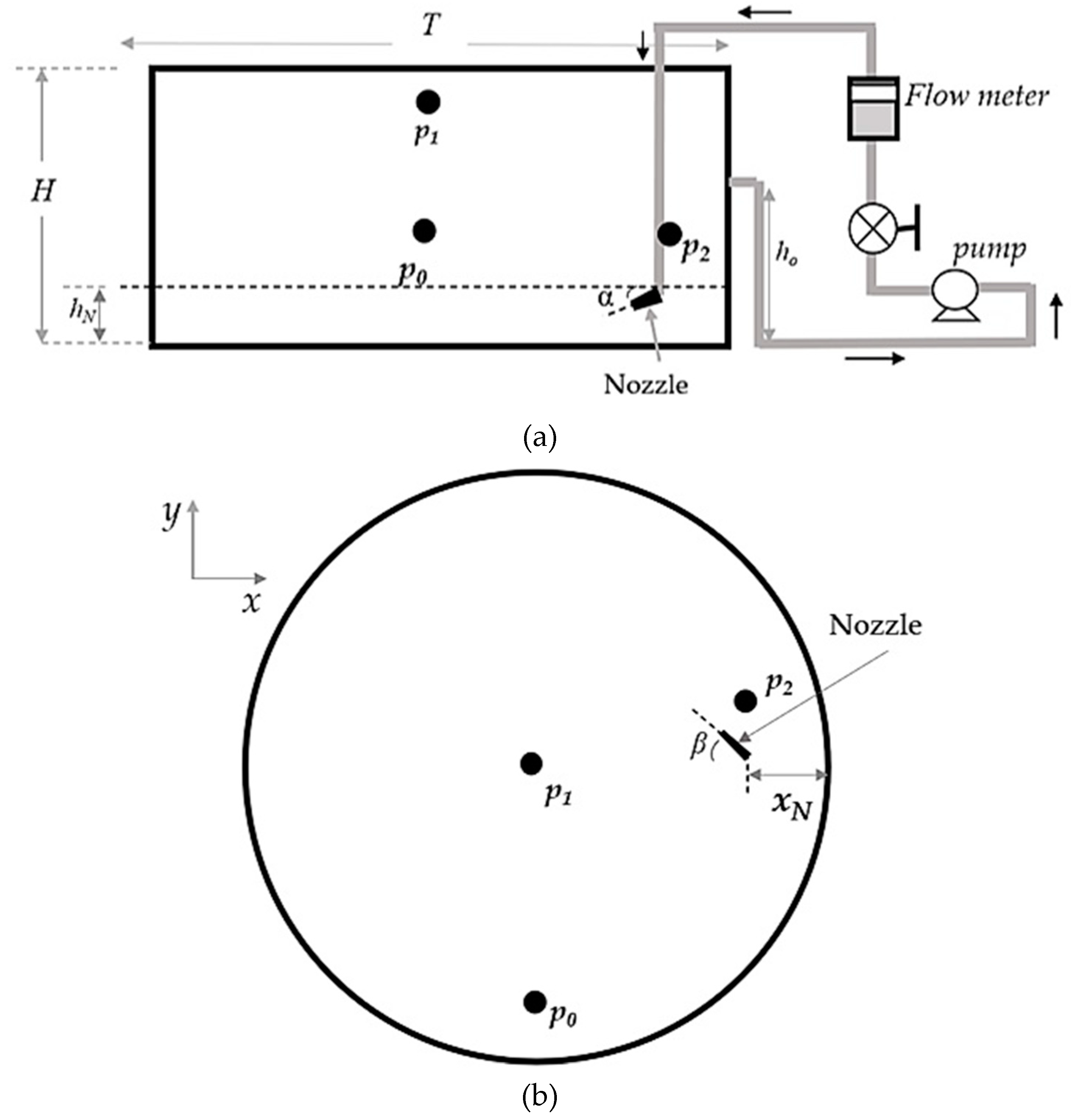
Figure 2.
schematics of various free jet pathlength for each jet nozzle vertical inclination.
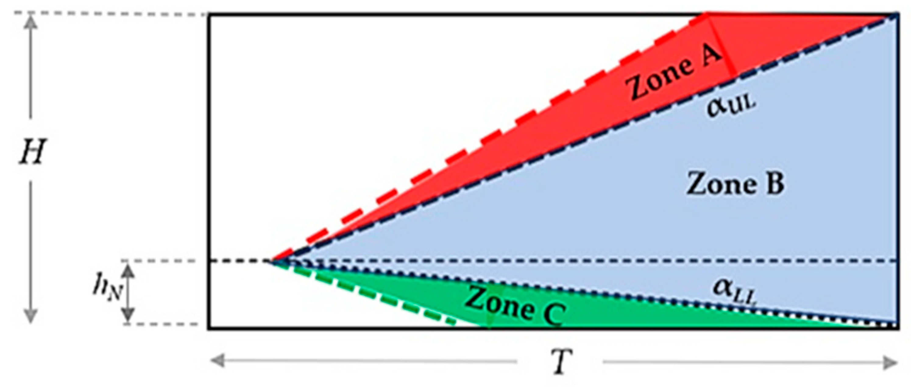
Figure 3.
Comparison of experimental mixing time data at 0° ≤ α ≤ 35° and β = 0° with mixing time predicted by the previous models.
Figure 3.
Comparison of experimental mixing time data at 0° ≤ α ≤ 35° and β = 0° with mixing time predicted by the previous models.
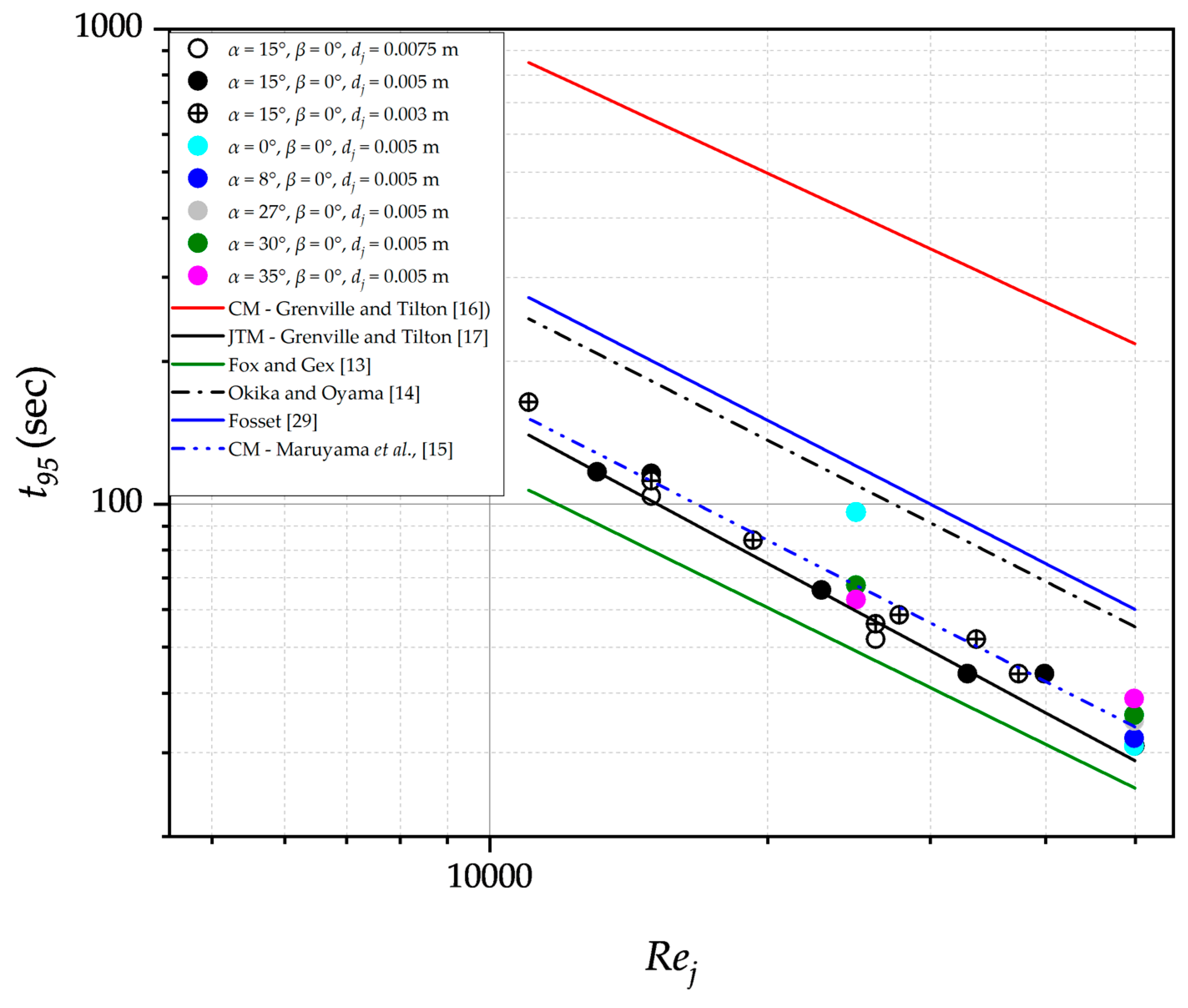
Figure 4.
Comparison of experimental mixing time data at α = 30° and β = 60° with mixing time predicted by the previous models.
Figure 4.
Comparison of experimental mixing time data at α = 30° and β = 60° with mixing time predicted by the previous models.
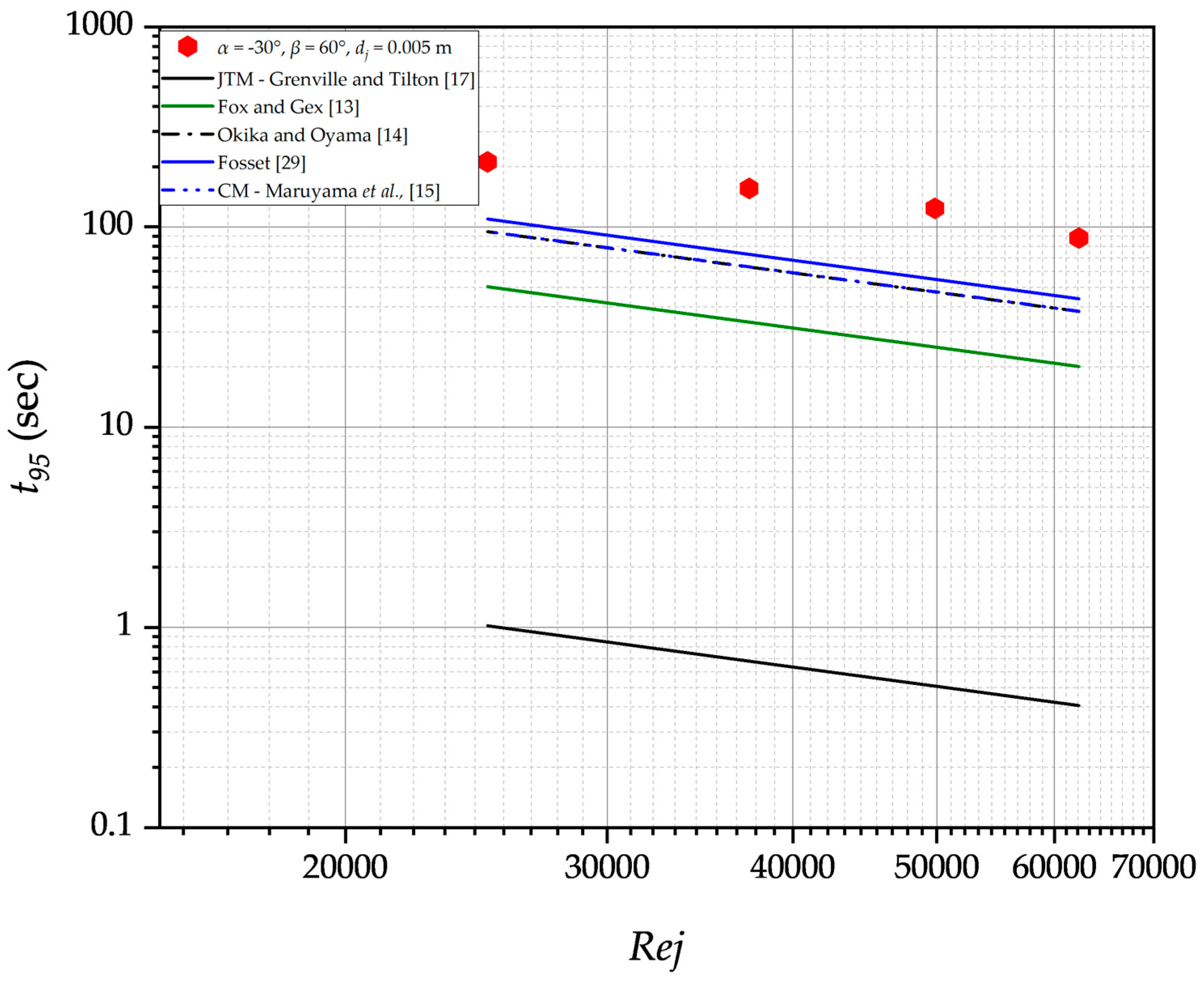
Figure 5.
Mixing time (t95) versus at Rej = 14,955–62,312.
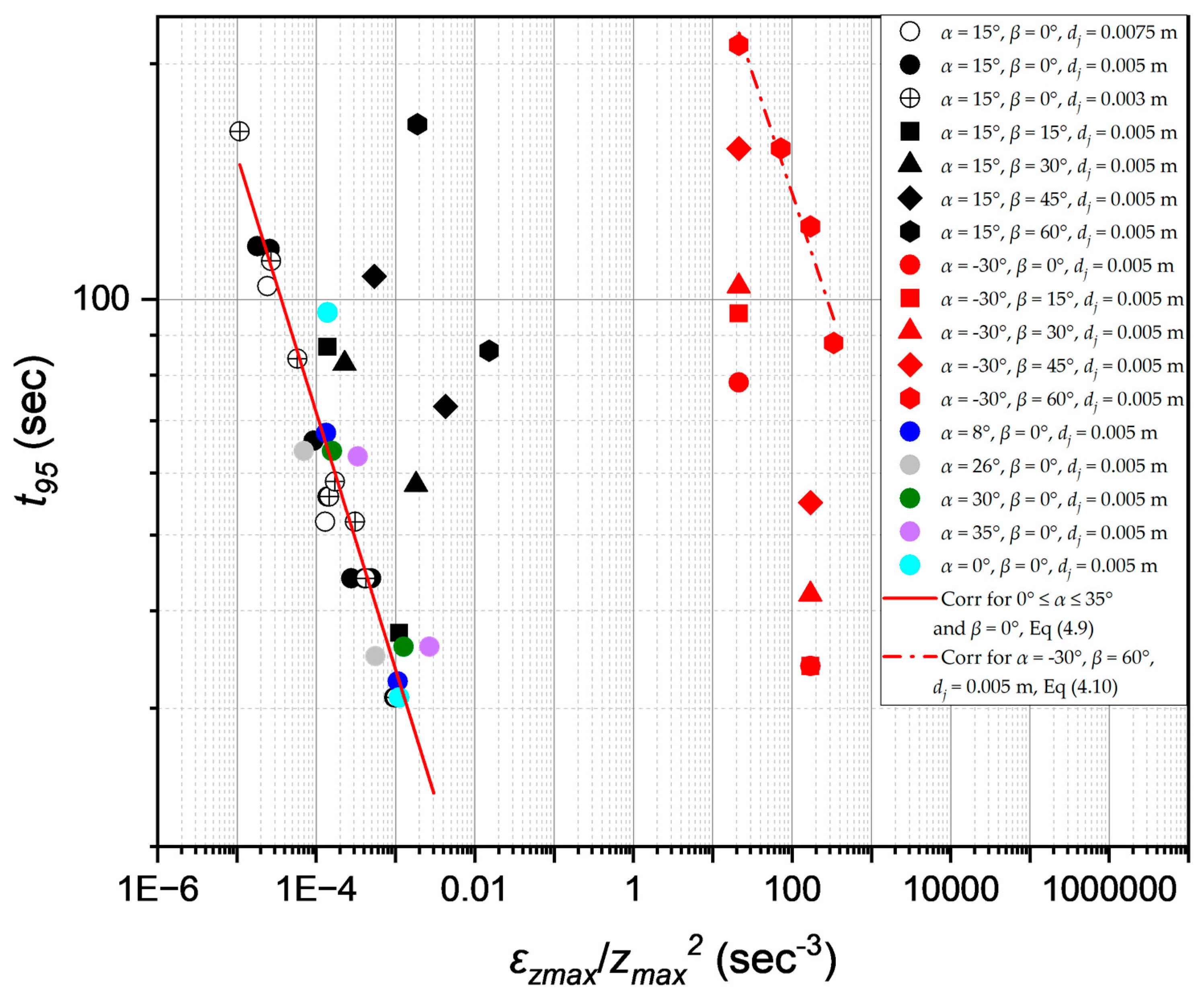
Figure 6.
Plots of normalised concentration of the fluorescein tracer fluid measured by probe p0 when the tracer fluid was added close to the tank wall uj = 5 ms-1, dj = 0.005 m, at Rej = 24925 (a) α = 15°, β = 0° (b) α = 30°, β = 60°.
Figure 6.
Plots of normalised concentration of the fluorescein tracer fluid measured by probe p0 when the tracer fluid was added close to the tank wall uj = 5 ms-1, dj = 0.005 m, at Rej = 24925 (a) α = 15°, β = 0° (b) α = 30°, β = 60°.
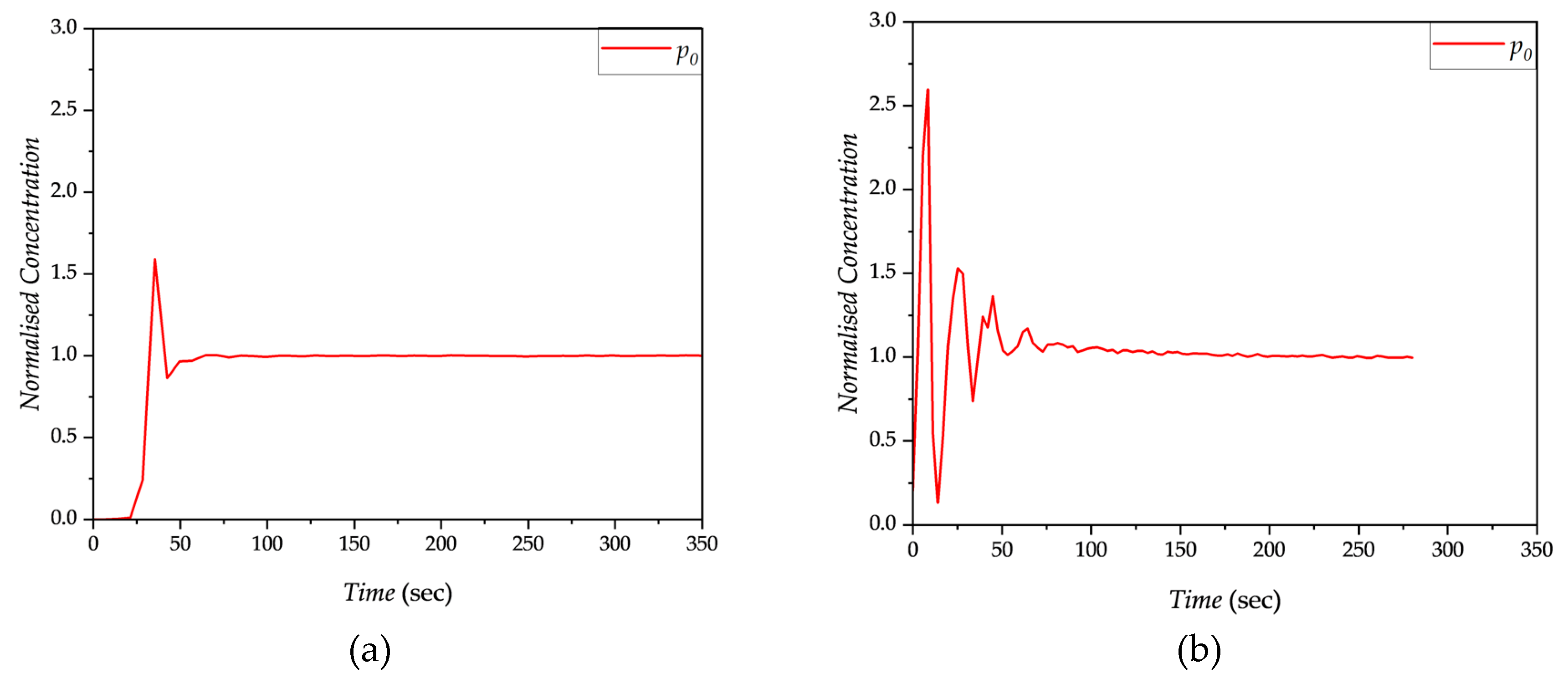
Figure 7.
Mixing time (t95) as a function of Circulation time ) at Rej = 14,955–62,312.
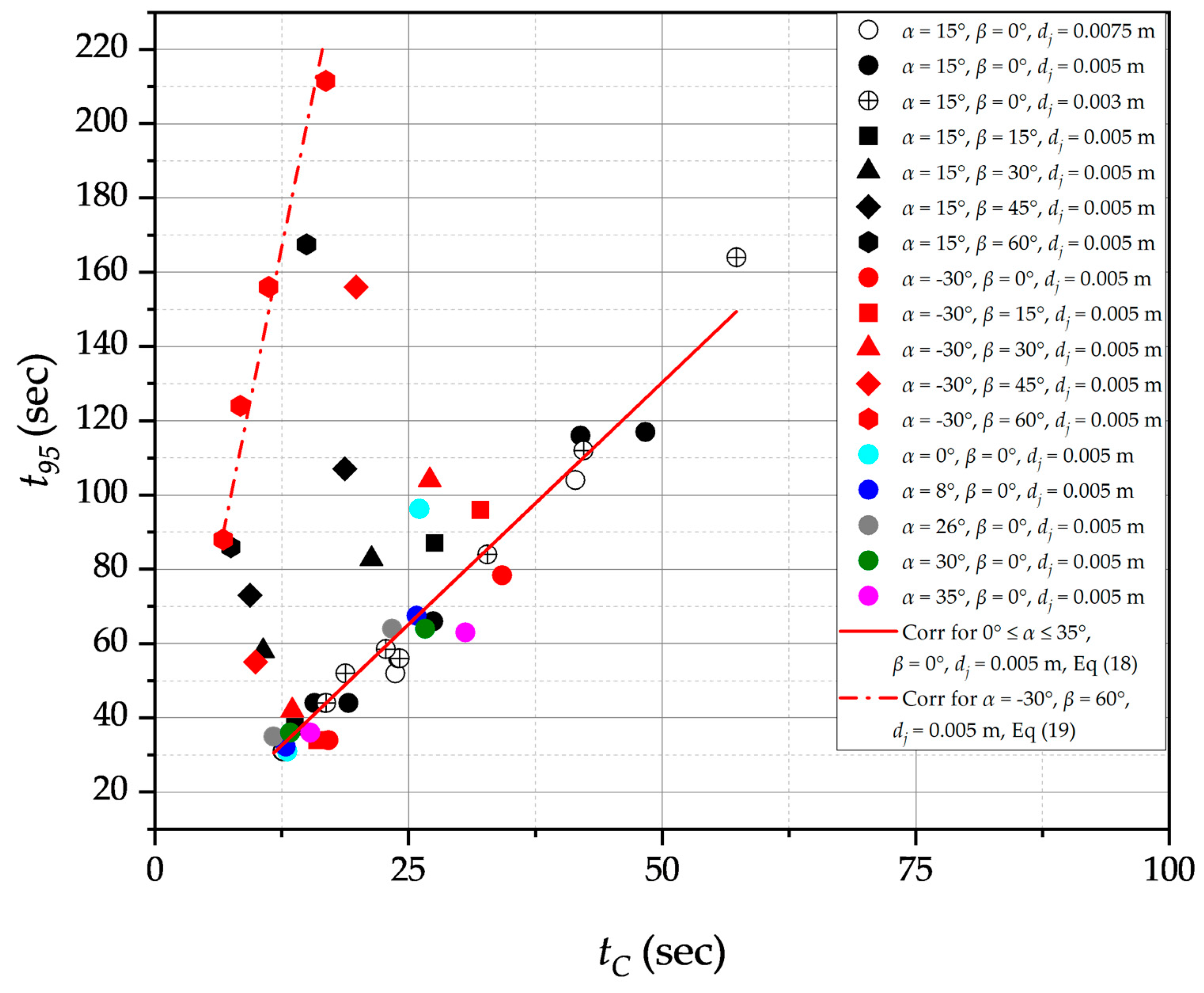
Figure 8.
Dimensionless Circulation time as a function of nozzle horizontal inclination (β).
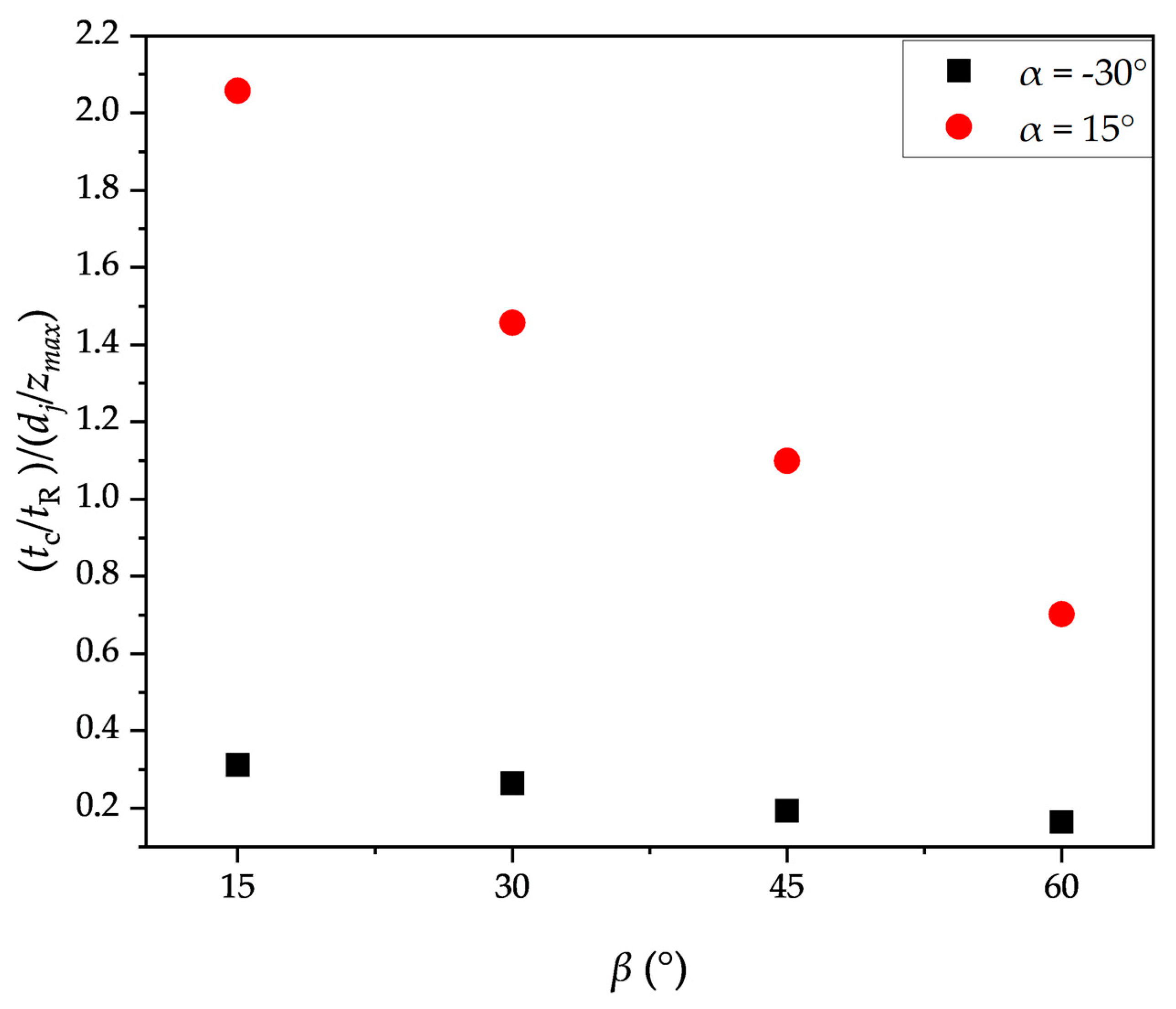
Figure 9.
Impacts of variation in horizontal inclination (β) of the nozzle on mixing time (t95) at fixed vertical inclinations (α).
Figure 9.
Impacts of variation in horizontal inclination (β) of the nozzle on mixing time (t95) at fixed vertical inclinations (α).
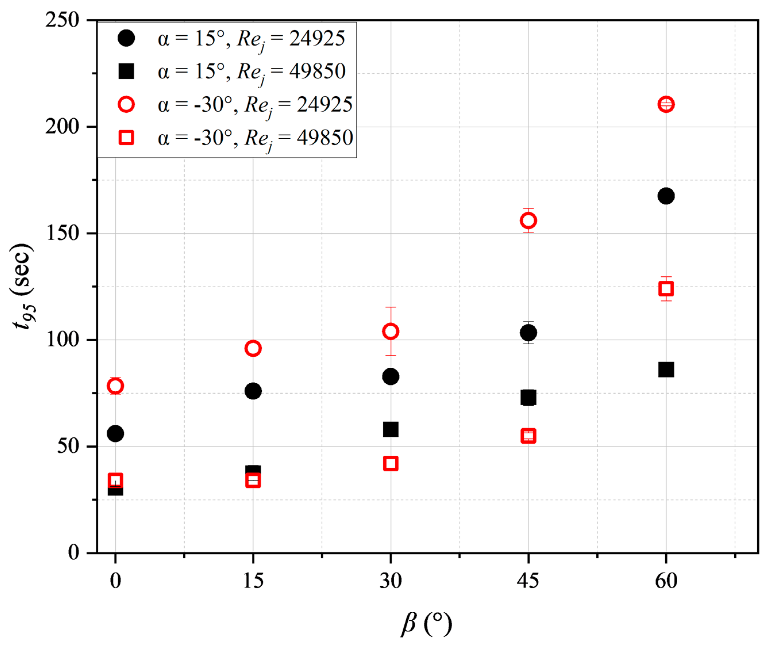
Figure 10.
Impacts of variation of the jet nozzle vertical inclination (α) on mixing time (t95) at fixed horizontal positions (β = 0) for dj = 0.005 m.
Figure 10.
Impacts of variation of the jet nozzle vertical inclination (α) on mixing time (t95) at fixed horizontal positions (β = 0) for dj = 0.005 m.
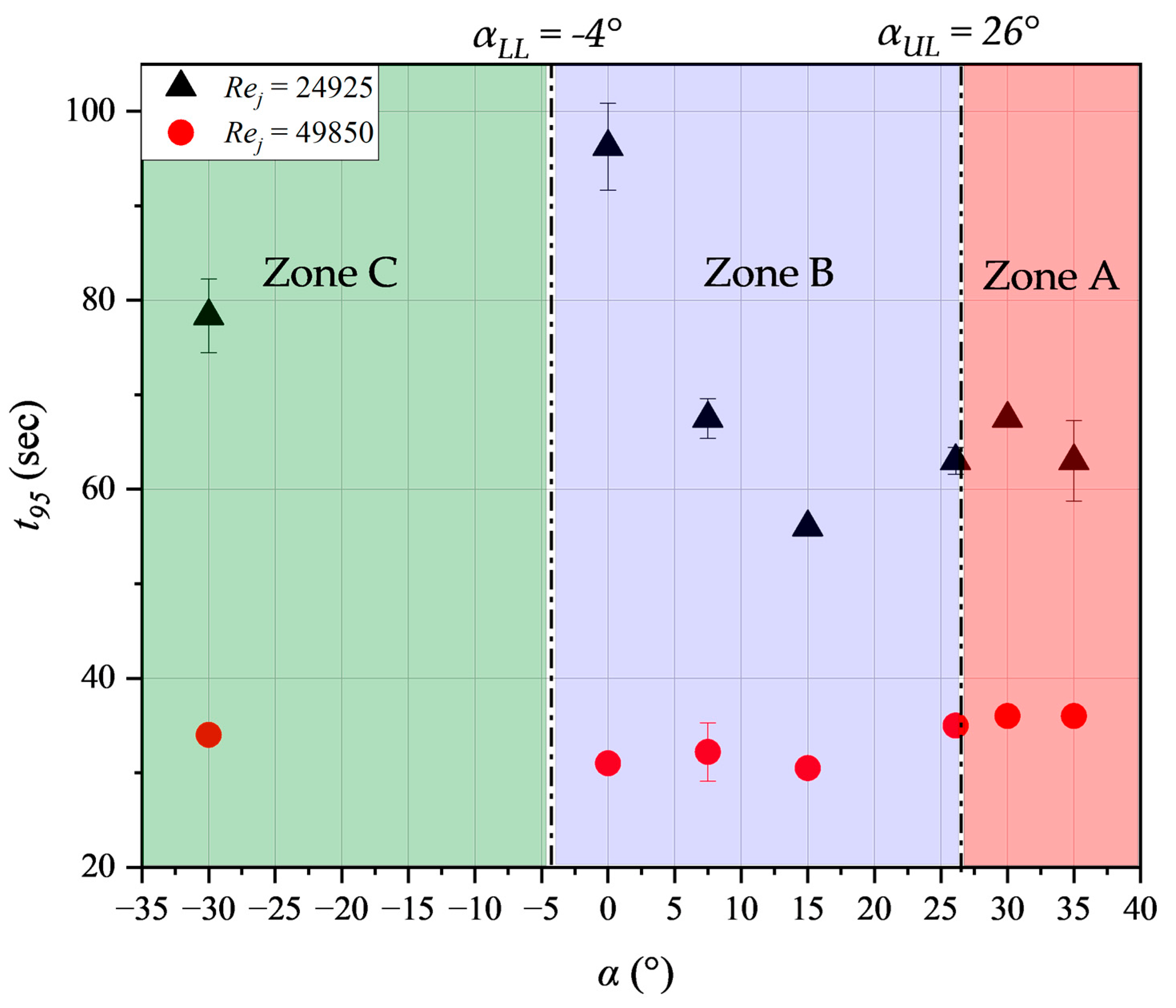
Figure 11.
Mixing time (t95) plotted as a function of Jet Length (Free jet Pathway) at dj = 0.005 m for various jet installation positions (a) At Rej = 24925 (b) At Rej = 49850.
Figure 11.
Mixing time (t95) plotted as a function of Jet Length (Free jet Pathway) at dj = 0.005 m for various jet installation positions (a) At Rej = 24925 (b) At Rej = 49850.
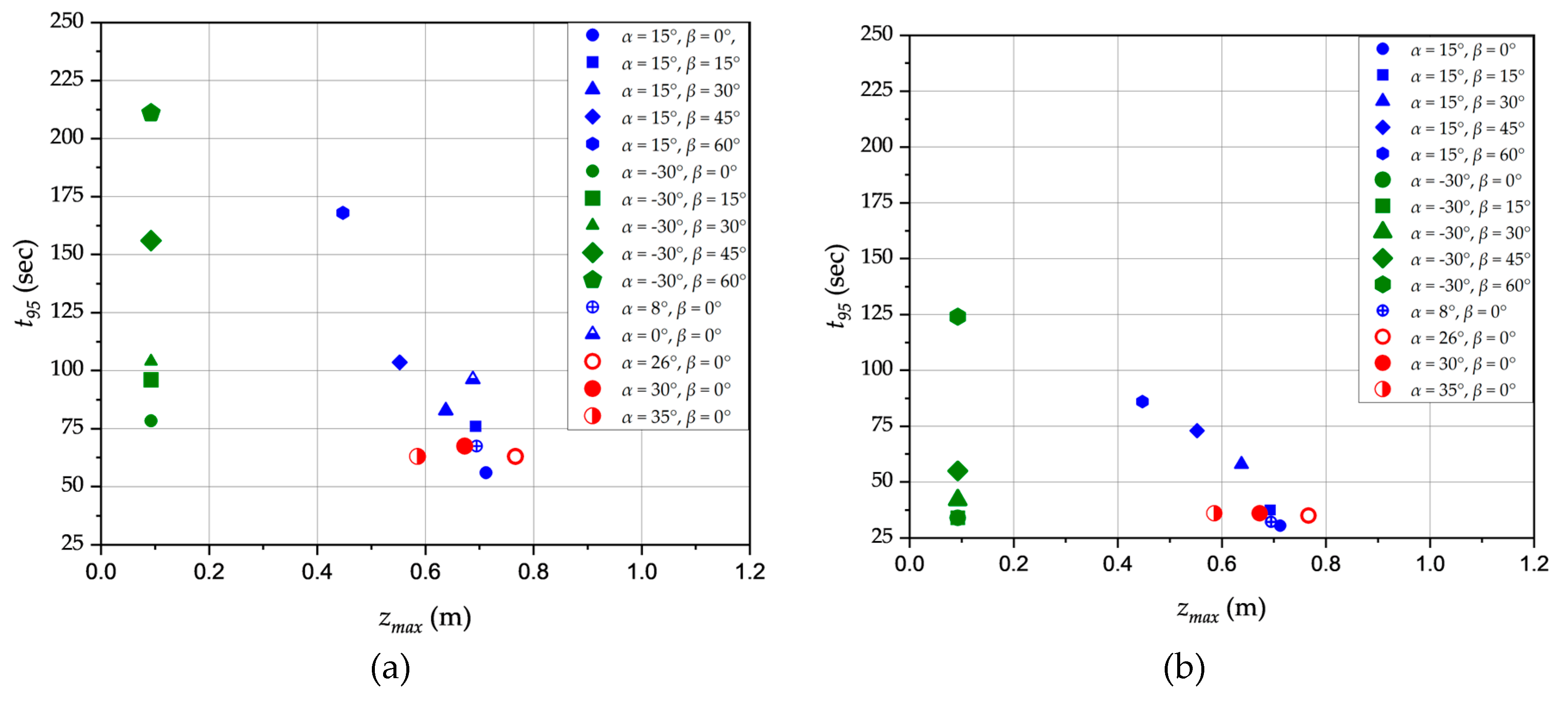
Figure 12.
Plot of mixing time (t95) as a function of jet velocities for dj = 0.003 m, 0.005 m, and 0.0075 m at α = 15° and β = 0°.
Figure 12.
Plot of mixing time (t95) as a function of jet velocities for dj = 0.003 m, 0.005 m, and 0.0075 m at α = 15° and β = 0°.
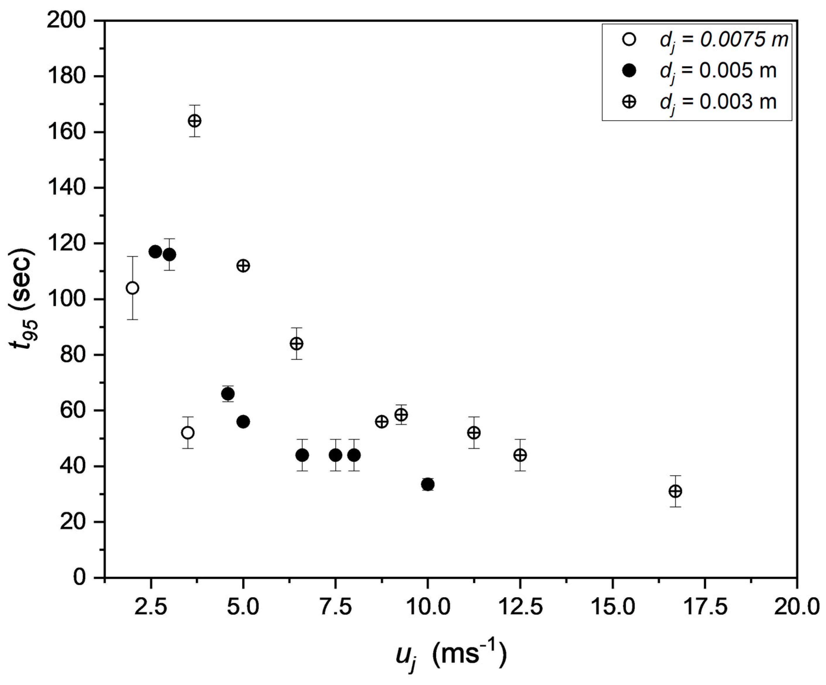
Figure 13.
(a) Plot of mixing time (t95) as a function of jet-power input α = 15° and β = 0° (b) Log-log plot of mixing time (t95) as a function of jet flow momentum at α = 15°, 30° and β = 0°, 15°, 30°, 45° and 60°.
Figure 13.
(a) Plot of mixing time (t95) as a function of jet-power input α = 15° and β = 0° (b) Log-log plot of mixing time (t95) as a function of jet flow momentum at α = 15°, 30° and β = 0°, 15°, 30°, 45° and 60°.
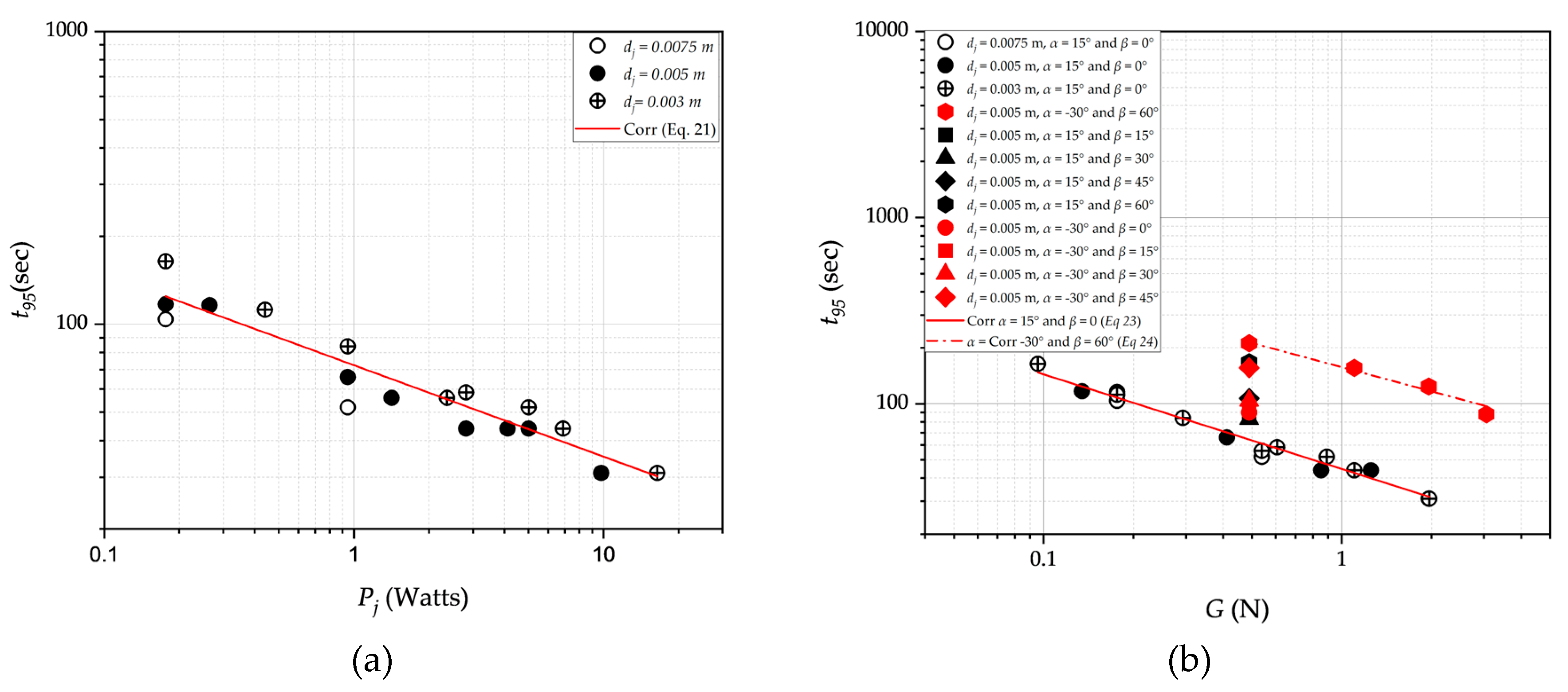

Table 1.
Dimensions of the tank and nozzle for the experimental setup.
| Parameter | Symbol | Value (m) |
|---|---|---|
| Tank diameter | T | 0.780 |
| Liquid height | H | 0.390 |
| Nozzle diameter | dj | 0.003, 0.005, 0.0075 |
| Nozzle clearance from side wall | XN | 0.085 |
| Nozzle clearance from tank bottom | hN | 0.050 |
| Outlet clearance | hO | 0.192 |
| Vertical inclination of nozzle | α | 35°, 30°, 26°, 15°, 8°, 0°, 30° |
| Horizontal inclination of nozzle | β | 0°, 15°, 30°, 45°, 60° |
Table 2.
Dimensionless Mean Circulation time for various nozzle positions.
| α (°) | β (°) | dj (m) | zmax (m) | |
|---|---|---|---|---|
| 30 | 0 | 0.005 | 0.093 | 0.32 |
| 15 | 0.005 | 0.093 | 0.31 | |
| 30 | 0.005 | 0.093 | 0.264 | |
| 45 | 0.005 | 0.093 | 0.193 | |
| 60 | 0.005 | 0.093 | 0.164 | |
| 15 | 0 | 0.0075 | 0.720 | 1.89* |
| 0 | 0.005 | 0.712 | 1.89* | |
| 0 | 0.003 | 0.707 | 1.89* | |
| 15 | 0.005 | 0.6930 | 2.06 | |
| 30 | 0.005 | 0.638 | 1.46 | |
| 45 | 0.005 | 0.552 | 1.10 | |
| 60 | 0.005 | 0.447 | 0.70 | |
| 0 | 0 | 0.005 | 0.688 | 1.89* |
| 8 | 0 | 0.005 | 0.694 | 1.89* |
| 26 | 0 | 0.005 | 0.766 | 1.89* |
| 30 | 0 | 0.005 | 0.673 | 1.89* |
| 35 | 0 | 0.005 | 0.585 | 1.89* |
* Averaged k value from similar tank geometries and nozzle positions from Maruyama et al.[11].
Disclaimer/Publisher’s Note: The statements, opinions and data contained in all publications are solely those of the individual author(s) and contributor(s) and not of MDPI and/or the editor(s). MDPI and/or the editor(s) disclaim responsibility for any injury to people or property resulting from any ideas, methods, instructions or products referred to in the content. |
© 2023 by the authors. Licensee MDPI, Basel, Switzerland. This article is an open access article distributed under the terms and conditions of the Creative Commons Attribution (CC BY) license (http://creativecommons.org/licenses/by/4.0/).
Copyright: This open access article is published under a Creative Commons CC BY 4.0 license, which permit the free download, distribution, and reuse, provided that the author and preprint are cited in any reuse.


