Reconstructing the Global Stress of Marine Structures Based on Artificial Intelligence

Preprint

Article

Reconstructing the Global Stress of Marine Structures Based on Artificial Intelligence

Altmetrics

Downloads

210

Views

Comments

A peer-reviewed article of this preprint also exists.

Tao Zhang

Jiajun Hu^*,

Erkan Oterkus,

Selda Oterkus,

Xueliang Wang,Zhentao Jiang,Qua Zhu,

Jiajun Hu^*,

Xueliang Wang,Zhentao Jiang,Qua Zhu,

Guocai Chen

This version is not peer-reviewed

Submitted:

07 June 2023

Posted:

08 June 2023

You are already at the latest version

Alerts

Abstract

This paper proposes an AI-based approach to overcome the limitations of the SHM system in measuring global stress with limited sensors. Feature elements are selected based on correlation analysis among finite elements and used as stress-measured points. An ANN is used to establish the solution relationship between the feature and correlation elements. The proposed method is applied to the connector structure of an offshore platform, and an optimal ANN is established to optimize accuracy by considering factors like the number of sensors, neural network framework, and convergence criteria. The accuracy of the ANN is verified through a real-scale model test, demonstrating 93.6% accuracy. This technology represents a significant advancement, enhancing the practicality of the structural health monitoring (SHM) system from “point monitoring" to “field monitoring".

Keywords:

Subject: Engineering - Marine Engineering

1. Introduction

To ensure the safety of marine equipment during operation, Structural Health Monitoring (SHM) technology has been developed. This technology utilizes various sensors to collect parameters related to structural mechanics. By using pre-designed algorithms, it evaluates the structure’s condition, reliability, and durability, and triggers early alerts when the structural condition is severely abnormal. This helps to provide a basis and guidance for structural maintenance and support management decisions[1]. However, in engineering applications, the SHM system can only provide primary safety warnings since the limited number of sensors cannot cover all areas where structural failure may occur.

Therefore, researchers have conducted extensive research to explore methods for reconstructing the global stress of structures using a few discrete stress sensors. This is done with the aim of obtaining more mechanical response details under operational conditions. In 1995, Haugse et al. proposed the modal method[2], which uses the modal coordinates of the structure as weighting values for the overall structural modes. This method allows obtaining the transformation matrix from the stress to the displacement field. By utilizing discrete stress sensors placed at specific points, the structural deformation can be reconstructed. The key concept is to view structural deformation as a linear combination of various modal orders. The accuracy of the reconstruction is significantly influenced by the accuracy of modal analysis, and this method is typically used for damage identification in structures that have been damaged. In 2007, Ko et al. introduced the Ko displacement theory[3,4,5], which is based on the classical Bernoulli-Euler beam theory. This theory assumes that the bending deformation of each small section of the beam is solely caused by the bending moment, and it establishes the relationship between the bending moment and strain. By integrating the measured axial strain twice, the deformation of the beam structure can be determined. This method is applicable to the reconstruction of unidirectional structural deformation.

In 2003 and 2005, Tessler and Spangler proposed the inverse Finite Element Method (iFEM) [6,7,8,9]. This method divides the structure into one-dimensional, two-dimensional, and three-dimensional elements, conducts discrete solutions by placing stress sensors at specific locations, and then assembles them into an overall matrix to obtain the global stress field through restructuring [6,7,8,9]. Oterkus et al. [10] utilized the iFEM method to calculate the global stress and bending of a parallel center body of an overturned bulk carrier using the iQS4 element [11], which demonstrated the practicality of the iFEM technology for bulk carriers. In addition, numerous researchers have explored the deformation reconstruction of beams, frames, plates, and shells using the iFEM method [12].

Despite the potential benefits of the iFEM method, such as its ability to reconstruct the stress and strain fields of various structures, the high reconstruction cost for the strain field of complex curved surface structures is a challenging issue. In recent years, alternative approaches have been proposed to overcome this issue [13,14,15,16,17]. For example, Lu et al [18] analyzed the steel structure of a gymnasium and established a mapping relationship between measured and estimated points through structural correlation analysis, providing an alternative approach for stress field reconstruction. In 2021, Zhang et al. [19] developed a two-dimensional stress distribution algorithm along a pipeline based on stress monitoring data of oil and gas pipelines, utilizing a BP neural network and particle swarm optimization algorithm. The algorithm accuracy was validated through examples, and it required no manual boundary establishment with less sensor quantity and fast solution speed. Cooper [20] introduced a hybrid approach combining Artificial Neural Network (ANN) and FE modelling for predicting static loads on a wing rib and a well-trained ANN can be used as an inverse problem solver for estimating loads on structures.

To address the challenge of obtaining the global stress of marine structures with limited stress sensors, this paper proposes an ANN approach for reconstructing the global stress of marine structures, focusing on the theoretical basis for measuring point selection and ANN architecture. Simulation calculation data and real-scale model test data verify the feasibility and accuracy of this method, enabling real-time visualization of the stress distribution status of complex structures and significantly enhancing the practicality of SHM equipment.

2. Correlation Analysis Among FE of Marine Structure

2.1. Correlation Between the Finite Elements

Based on the Finite Element theory, marine structures can be discretized into a certain number of finite elements. In the case of one- and two-dimensional structures, the stress changes of finite elements exhibit a degree of similarity or regularity on a global scale when external loads change. However, for spatial structures, the stress variation of finite elements presents a complex distribution. Furthermore, the global regularity of the finite elements decreases with the increasing complexity of the structure.

To describe the stress distribution of complex spatial marine structures, the structure can be divided into several subsets based on correlation analysis, wherein finite elements with similar or regular responses to external loads are sorted into the same subset. Representative finite elements are then selected from these subsets, which are called “feature elements”.

Based on Artificial Neural Networks, a relationship between the feature elements and the stress values of finite elements that show a significant correlation with them can be established. Consequently, the global stress data of the structure can be obtained by placing stress sensors on the feature elements.

2.2. Correlation Analysis Method

Consider a structure as a set of overall elements (S), and divide S into m finite elements (

e_{i}

). For n load steps, the whole elements stress response matrix X can be written as.

X = [x_{1} x_{2} x_{3} \dots x_{i} \dots x_{m}] = [\begin{matrix} \begin{matrix} x_{1} (1) & x_{2} (1) \\ x_{1} (2) & x_{2} (2) \end{matrix} & \begin{matrix} \dots & x_{i} (1) \\ \dots & x_{i} (2) \end{matrix} & \begin{matrix} \dots & x_{m} (1) \\ \dots & x_{m} (2) \end{matrix} \\ \begin{matrix} ⋮ & ⋮ \\ x_{1} (k) & x_{2} (k) \end{matrix} & \begin{matrix} ⋱ & ⋮ \\ \dots & x_{i} (k) \end{matrix} & \begin{matrix} ⋮ & ⋮ \\ \dots & x_{m} (k) \end{matrix} \\ \begin{matrix} ⋮ & ⋮ \\ x_{1} (n) & x_{2} (n) \end{matrix} & \begin{matrix} ⋮ & ⋮ \\ \dots & x_{i} (n) \end{matrix} & \begin{matrix} ⋱ & ⋮ \\ \dots & x_{m} (n) \end{matrix} \end{matrix}]

(1)

In Equation (1), the structural response of the finite element with the index i for n load steps is denoted as

x_{i} (n)

x_{i} = [x_{i} (1) x_{i} (2) \dots x_{i} (n)]

(2)

In Equation (2), where

i = 1, 2, \dots, m

, the similarity as the response of any two finite elements,

e_{i}

and

e_{j}

, for the same load steps in a spatial structure, covariance

Cov (x_{i}, x_{j})

can be used as a representation.

C o v (x_{i}, x_{j}) = E (x_{i} x_{j}) - E (x_{i}) E (x_{j})

(3)

In Equation (3),

E (x_{i})

and

E (x_{j})

represent the expected values of the two real random variables

x_{i}

and

x_{j}

, respectively. Due to the variables having different dimensions, their covariance can exhibit significant numerical differences. To address this, a dimensionless correlation analysis method such as the Pearson correlation coefficient, as shown in Equation (4), is introduced:

P_{i, j} = \frac{c o v (x_{i}, x_{j})}{σ_{i} σ_{j}}

(4)

with

c o v (x_{i}, x_{j}) = E (x_{i} - \bar{x_{i}}) (x_{j} - \bar{x_{j}}) = \frac{1}{n - 1} \sum_{k = 1}^{n} (x_{i} (k) - \bar{x_{i}}) (x_{j} (k) - \bar{x_{j}})

(5)

σ_{i} = \frac{1}{n - 1} \sum_{k = 1}^{n} {(x_{i} (k) - \bar{x_{i}})}^{2}

(6)

σ_{j} = \frac{1}{n - 1} \sum_{k = 1}^{n} {(x_{j} (k) - \bar{x_{j}})}^{2}

(7)

In Equations (4) to (7),

σ_{i}

is the variance of the response value of the finite element with index i for n load steps,

σ_{j}

is the variance of the response value of the finite element with index j for n load steps,

\bar{x_{i}}

is the mean response value of the finite element with index i for n load steps, and

\bar{x_{j}}

is the mean response value of the finite element with index j for n load steps. The correlation matrix P between any two finite elements

x_{i}

and

x_{j}

is given as follows.

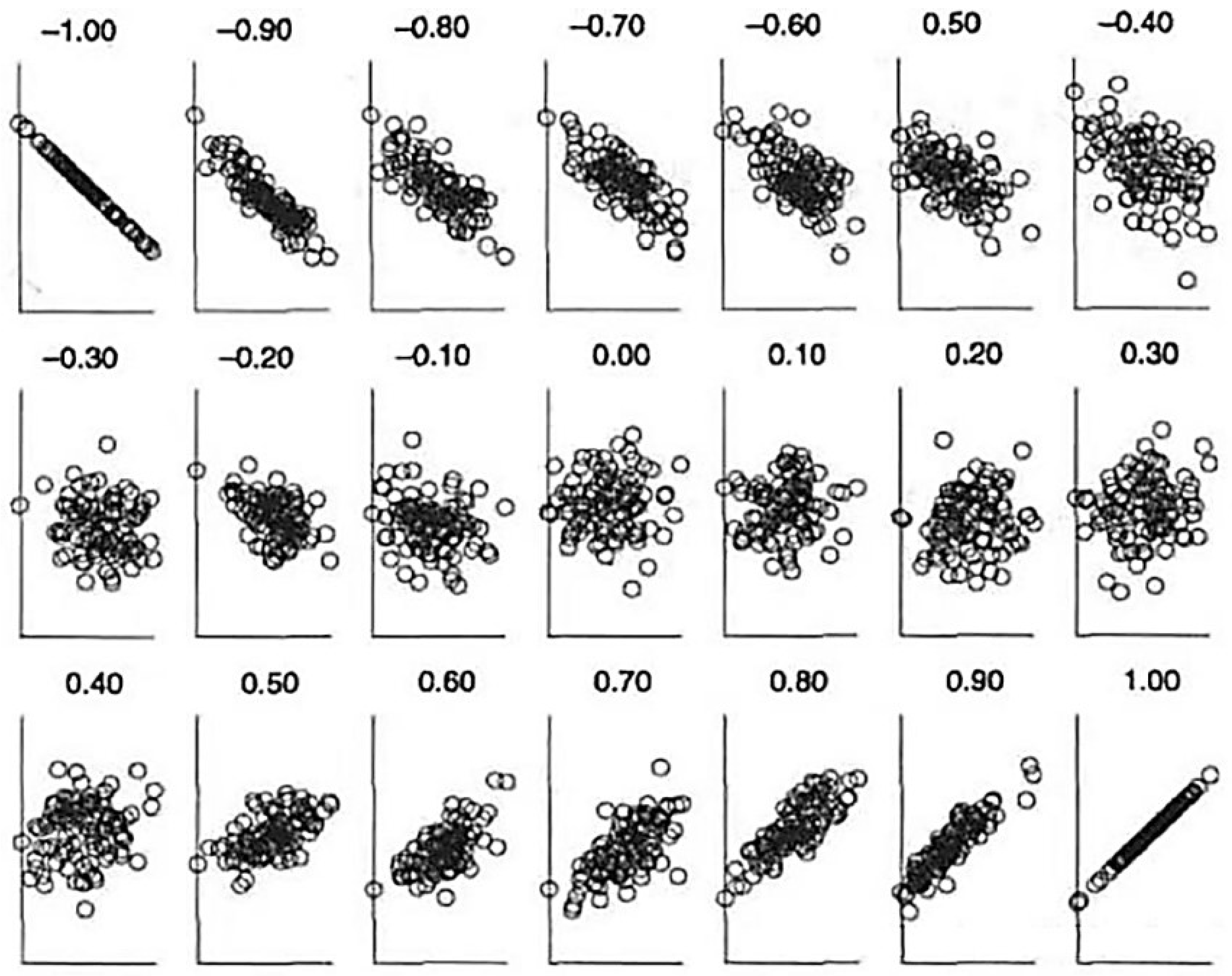
P = {[P_{ij}]}_{m \times m} = [\begin{matrix} \begin{matrix} p_{11} & p_{12} \\ p_{21} & p_{22} \end{matrix} & \begin{matrix} \dots & p_{1 j} \\ \dots & p_{2 j} \end{matrix} & \begin{matrix} \dots & p_{1 m} \\ \dots & p_{2 m} \end{matrix} \\ \begin{matrix} ⋮ & ⋮ \\ p_{i 1} & p_{i 2} \end{matrix} & \begin{matrix} ⋱ & ⋮ \\ \dots & p_{i j} \end{matrix} & \begin{matrix} ⋮ & ⋮ \\ \dots & p_{i m} \end{matrix} \\ \begin{matrix} ⋮ & ⋮ \\ p_{m 1} & p_{m 2} \end{matrix} & \begin{matrix} ⋮ & ⋮ \\ \dots & p_{m j} \end{matrix} & \begin{matrix} ⋱ & ⋮ \\ \dots & p_{m m} \end{matrix} \end{matrix}]

(8)

The correlation coefficient, p, has a range of values from -1 to 1, as demonstrated in Figure 1. When

p = 1

x_{i}

and

x_{j}

are perfectly positively correlated, whereas when

p = - 1

x_{i}

and

x_{j}

are perfectly negatively correlated. The strength of the correlation increases with the absolute value of p, and weakens as p approaches 0.

Typically, a value of

p_{i j} > 0.95

indicates a significant correlation between

x_{i}

and

x_{j}

. If finite elements within a spatial structure exhibit a significant correlation in load feedback, they can be grouped together, resulting in the partitioning of the overall structure S into k subsets T.

S = \{T_{1} T_{2} \dots T_{i} \dots T_{k}\}

(9)

In the given Equation (9), i ranges from 1 to k. Representative finite elements,

v_{i}

, are selected from each subset

T_{i}

to form a set of feature elements.

V = v_{1}, v_{2}, \dots, v_{i}, . ., v_{k}

(10)

A relationship between the set of feature elements V and the stress values S of finite elements that exhibit significant correlation with V can be established using neural networks. By installing stress sensors on the feature elements, global stress data of the structure can be obtained.

3. Neural Networks Architecture Method

3.1. Principles of Neural Networks

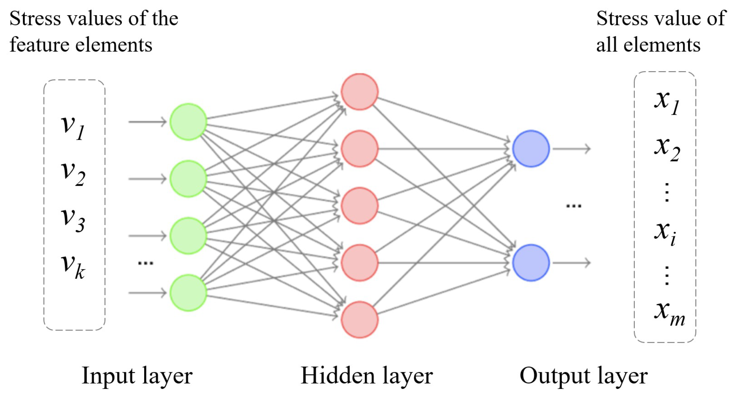
Artificial neural networks are AI algorithms that fit complex real-world patterns by training a large number of hidden parameters (hidden layers) to achieve mapping from input variables to output variables. The diagram of a single network structure is shown in Figure 2. In this paper, the stress values of the feature elements set

V

are used as the input layer of the neural network, and the stress values of all finite elements of the overall structure

S

are used as the output layer. A supervised learning network is established with reliable input and output data as the training sample set. The neural network learning system adjusts system parameters based on the difference (error signal) between known output and actual output, ultimately establishing a matching relationship network between the characteristic points and the overall structural stress field.

3.2. Initial ANN for Global Stress

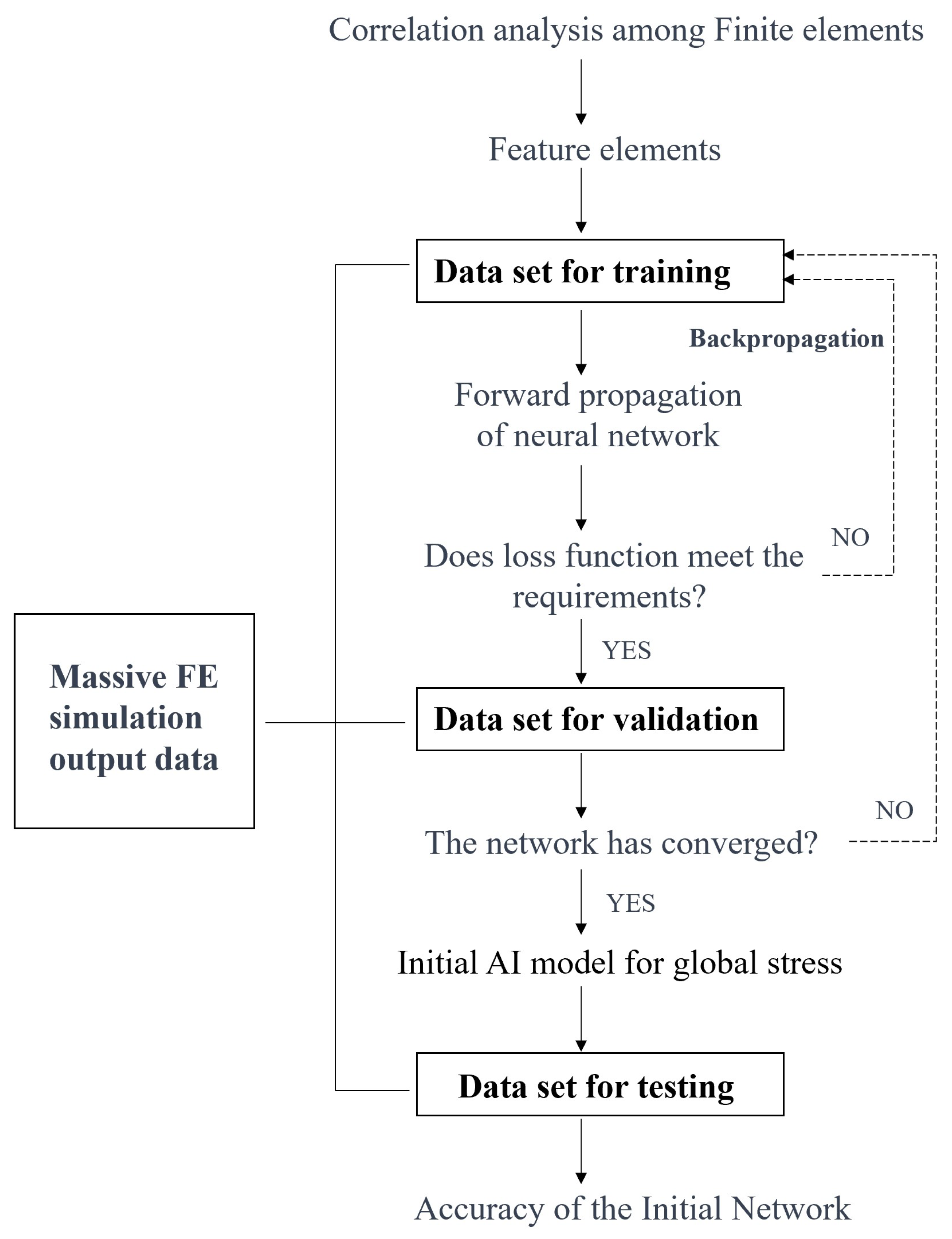
As it is not possible to obtain spatial structural global stress data through direct measurements, finite element simulation data is selected as the training sample to establish an initial global stress neural network (referred to as the “initial network” below), following the process shown in Figure 3. The sample data is divided into three non-overlapping parts: the training set, the validation set, and the test set.

The training set is used to train the network to enable it to obtain the overall stress field. From the training set, the response values of all finite elements are set as the output (referred to as “target data”). Using forward propagation, the data of the characteristic elements is set as the input, and a multi-layered weighted sum matrix is established to calculate the output forecast data. When the difference between the predicted data and the target data does not meet the error requirements, the system parameters are adjusted using the backpropagation algorithm, ultimately establishing a solution network between the characteristic elements and the overall elements.

The validation set is used to determine the current network’s ability to obtain the global stress, evaluate the convergence of the network during the training process, and serve as a basis for determining whether to end network training.

The test set is used to evaluate the performance of the trained network in tasks to obtain stress and quantitatively measure the network’s dispersion in predicting global stress.

3.3. Fine-tuning of Initial Network

The initial global stress ANN was established using simulation output data, and it requires fine-tuning before it can be deployed to physical structures. The reasons are as follows: (1) there are slight differences between the material properties, boundary conditions, mesh partitioning, load simulation, and other information used in simulation calculations and the real physical world; (2) the actual measurement point location and orientation may have geometric errors compared to the ideal placement state.

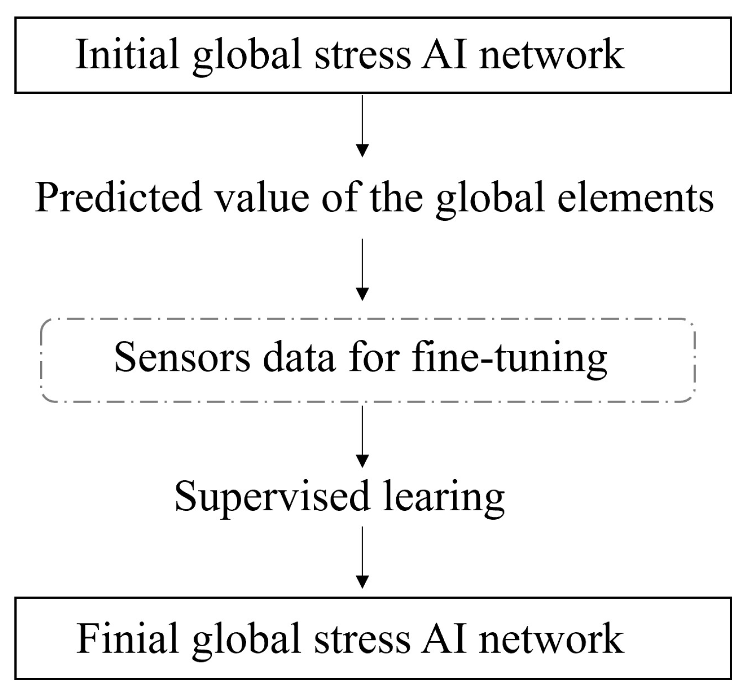
The Figure 4 illustrates the process of fine-tuning the initial network. To fine-tune the initial network for deployment to physical structures, measurement points are randomly selected from areas of high stress. The actual sensor data is compared to the predicted values of the initial network, and a fine-tuning matrix is added outside the output layer of the network through supervised learning. This process creates the final artificial intelligence network (referred to as the "final network") that can be deployed to physical structures.

The process of fine-tuning the initial network is similar to the process of establishing the initial network, as both require a dataset for error comparison. The goal is to minimize the loss function through optimization algorithms and improve the ANN. The key difference is that the dataset for validation can be easily obtained from simulation output data at low cost during the establishment process, allowing for a larger number of elements to be used for validation. However, during the fine-tuning process, a much smaller number of elements are used for validation, which can potentially lead to the network being trapped in local optimization instead of achieving global optimization.

4. Reconstructing Global Stress for Connector Structure

4.1. Mechanical Analysis on the Connector Structure

The ocean platform utilized for scientific research comprises two semi-submersible platforms, wherein the primary platform is connected to the auxiliary platform through a pin joint, as depicted in Figure 5. During extreme sea conditions, the pin and connector are exposed to substantial shear forces [21,22,23,24], mandating real-time evaluation of the structure’s safety. This research endeavors to appraise the safety of the connector structure by deploying stress sensors on the connector structure’s surface, facilitating instantaneous determination of the stress distribution map. This map highlights high-stress regions and their corresponding magnitudes. 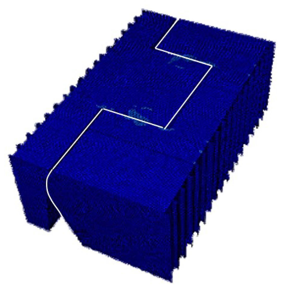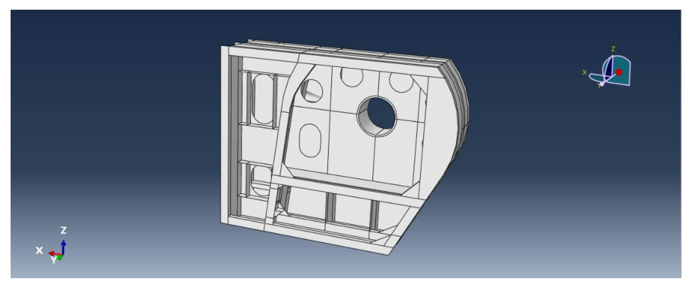The connector structure can be classified into single-ear and double-ear structures, as delineated in Figure 6. In this investigation, the single-ear connector is selected as the research subject. It is a complex three-dimensional curved surface structure, encompassing three layers of bulkheads, where the middle bulkhead is punctured with lightening holes, as depicted in Figure 7.

4.2. Data samples

The shear force of the pin joint can be applied to the connector structure at 360 degrees. Therefore, 3600 elastic phase calculation cases are conducted, including 100 load steps for 36 load directions (each 10 degrees apart). All the finite element stress data for all load cases are used as sample data, and they are randomly divided into training sets (2400 cases), validation sets (600 cases), and test sets (600 cases).

4.3. Selecting Feature Elements by Correlation Analysis

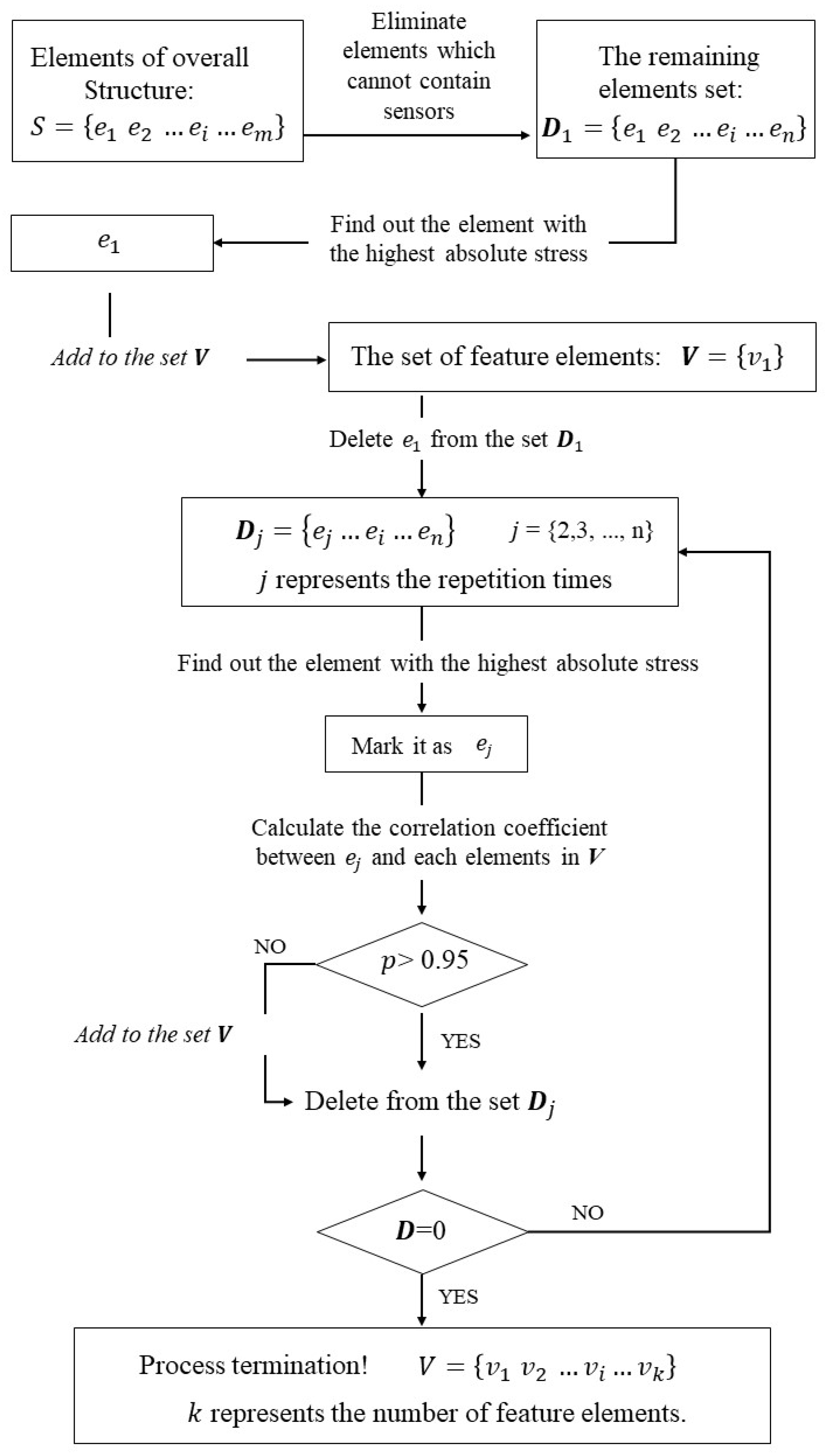
The overall finite elements are subjected to a correlation analysis using the Pearson correlation coefficient and the steps are illustrated in Figure 8.

(i) Eliminate the finite elements that cannot accommodate sensors from the overall structure. Then, sort the remaining finite elements (record the quantity as n in descending order based on their absolute stress values). The greater the absolute stress value, the more sensitive the finite element is to external loads. Placing sensors at these positions is advantageous for detecting minor changes in external loads and structural responses.

(ii) The finite element with the highest absolute stress value in D is chosen as the feature element

v_{1}

. Subsequently, the correlation coefficient

p_{i j}

between

v_{i}

and other elements

e_{j}

is sequentially calculated, where

j = {2, . . ., n}

, and j represents the repetition times. Based on Equations (4) to (8), the correlation matrix P of the finite element is obtained. If

p_{i j} > 0.95

e_{j}

is added to the set V.

(iii) The elements in S that are duplicated in V are removed to obtain the remaining set of elements D.

(iv) Repeat steps (ii) and (iii) until the number of remaining elements in set D reaches 0, then the selection process is completed. Thus, 50 feature elements are identified from 30,858 finite elements, as illustrated in Figure 9. The connector structure can be divided into 50 subsets accordingly.

4.4. Optimization of the Number of Stress Sensors

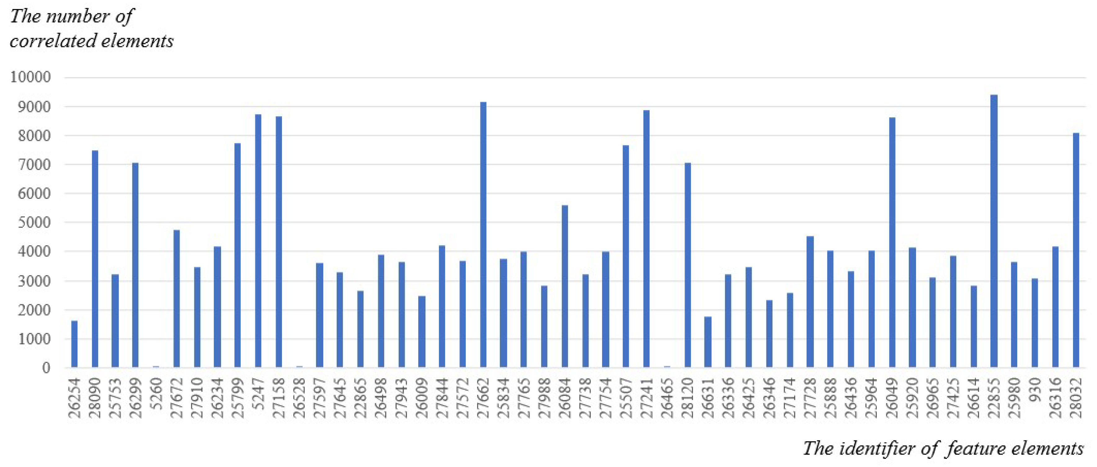
The 50 feature elements were sorted in descending order according to their stress amplitude, and the number of correlated elements for each feature element was counted, as shown in Figure 10. The results showed that the number of finite elements which have a correlation with the 50 feature elements was 220,905, exceeding the total number of entire elements, which was 30,858. This indicates that there are multiple intersections among the 50 subsets, and fewer feature units can be used to obtain the full-field stress distribution.

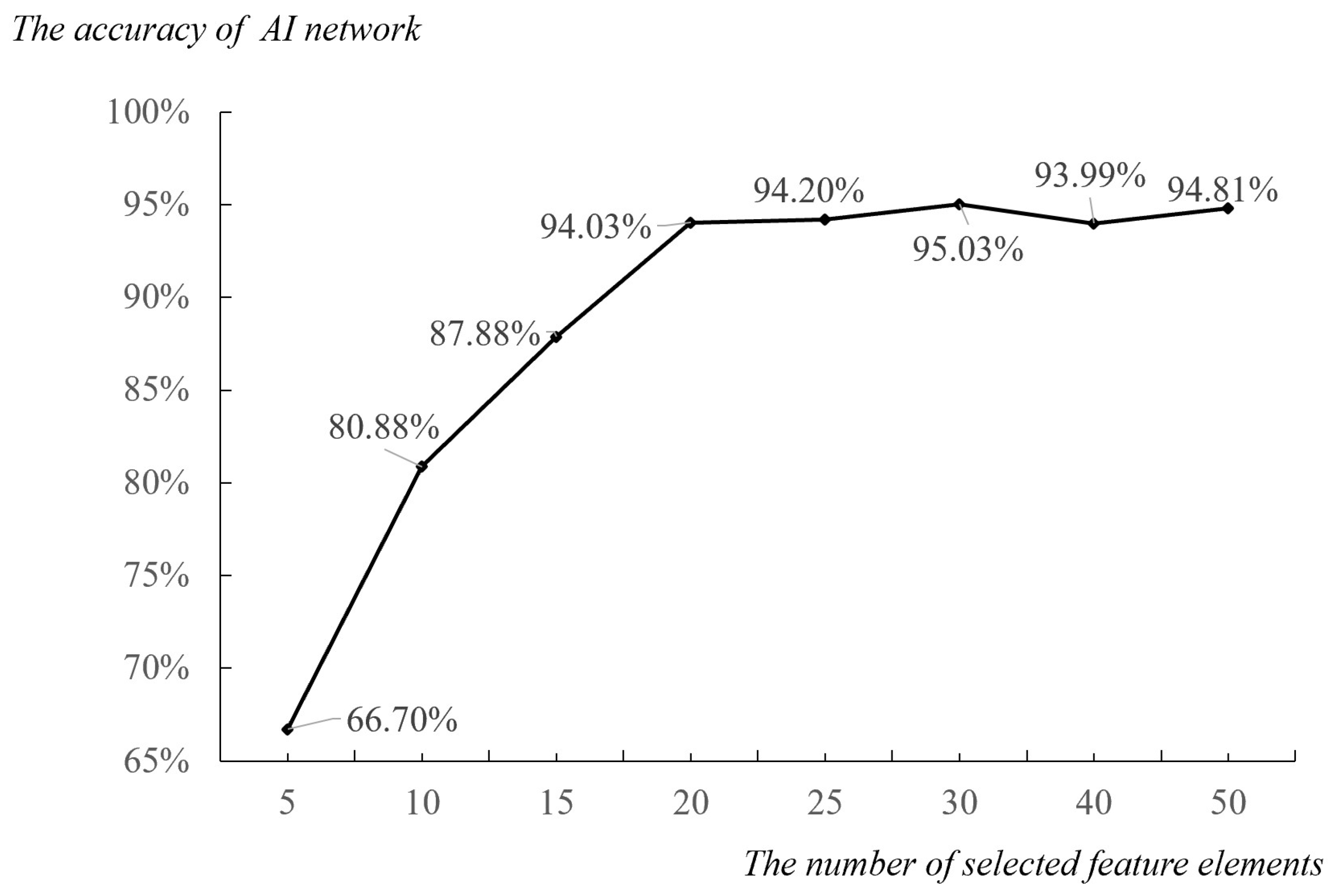
Subsequently, a neural network was trained for global stress by selecting 5, 10, 15, 20, 25, 30, 40, and 50 feature elements in descending order of their stress amplitude as input variables. The influence of different numbers of feature elements on the accuracy of global stress solutions was analyzed, and the results are shown in Figure 11. It was observed that as the number of feature elements gradually increased, the calculation accuracy also improved, and the algorithm accuracy was found to be stable when the number of selected feature elements was 20. This indicates that most of the finite elements in the connector structure are strongly correlated with the first 20 feature elements, and the global stress of the connector can be accurately obtained using these 20 feature elements.

4.5. Optimization of neural networks

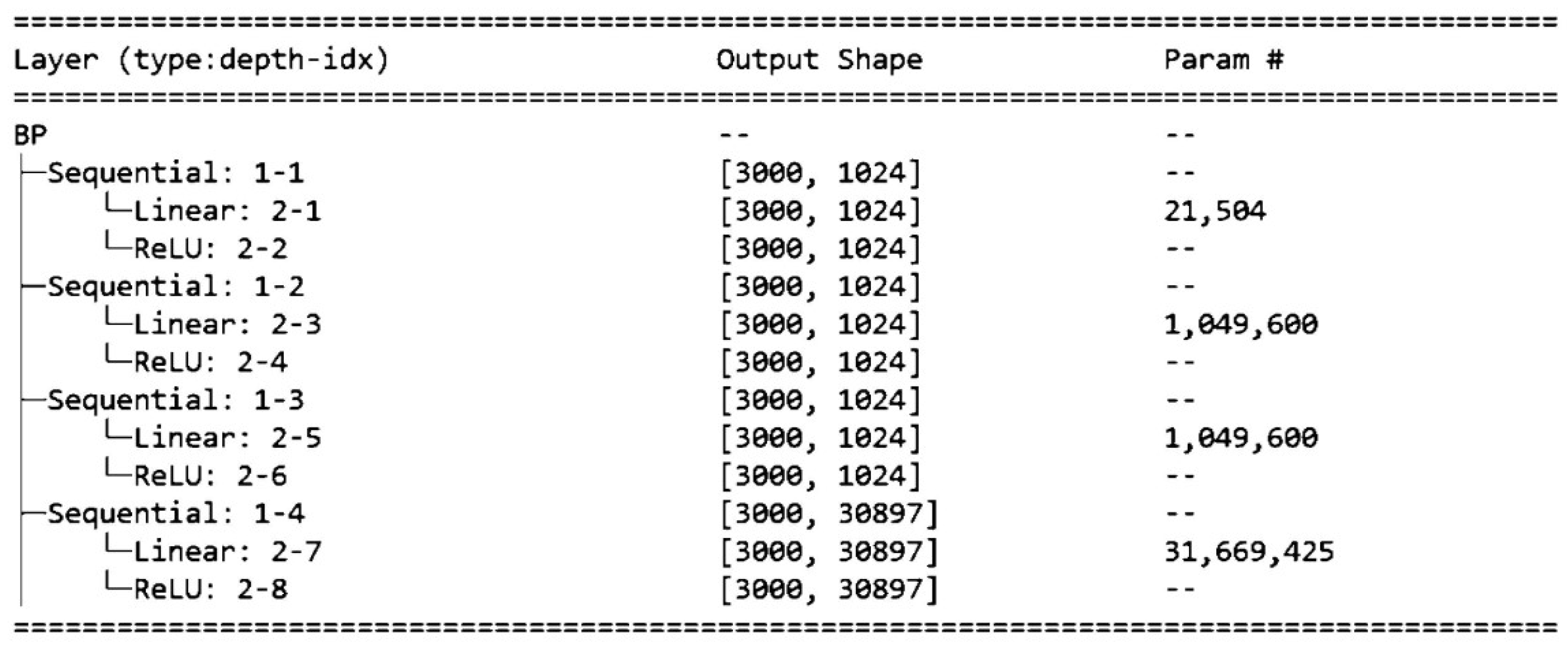
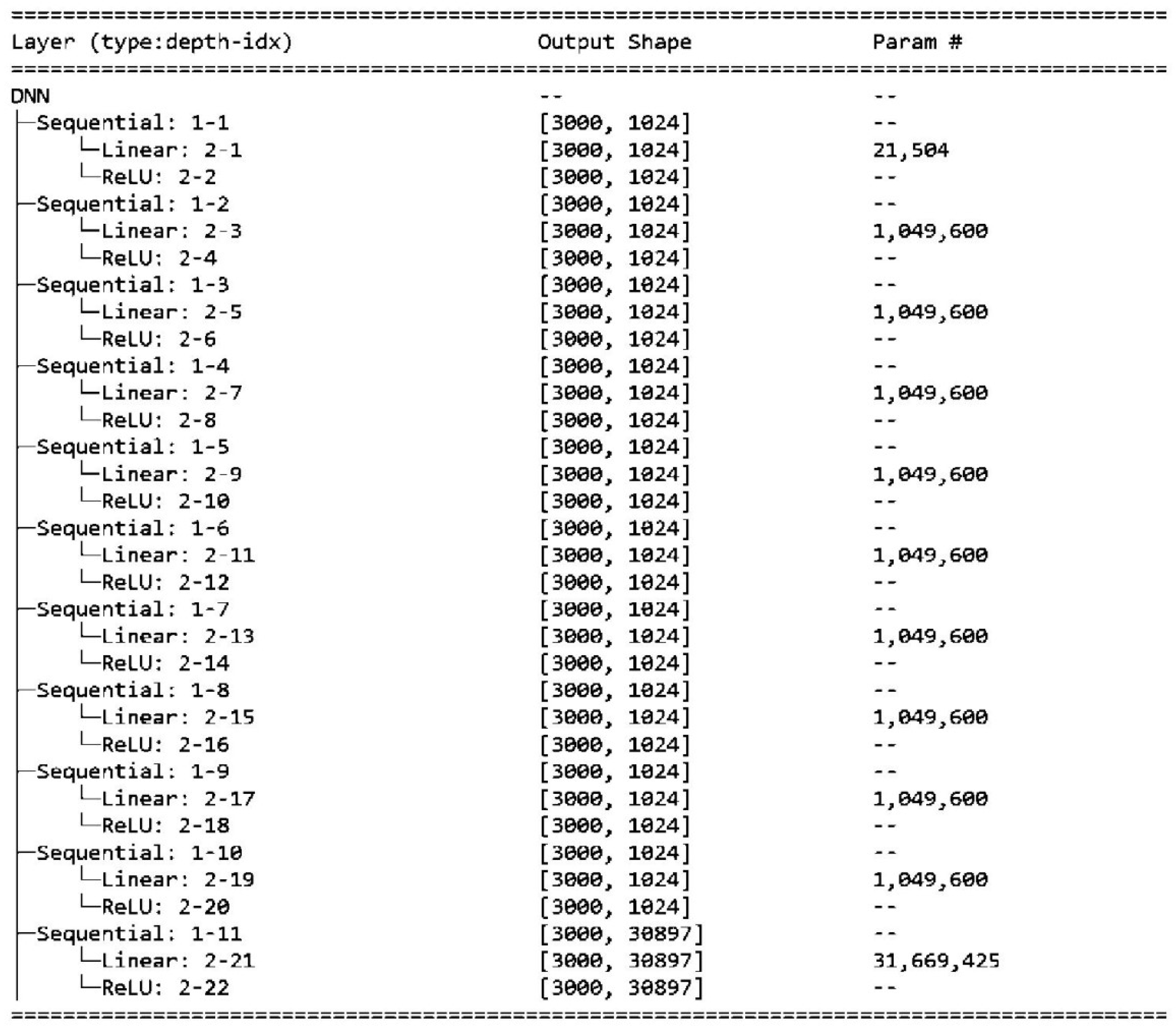
Different neural network architectures exhibit varying computational performance and accuracy in obtaining global stress. To conduct the experiments, four commonly used neural network architectures, namely BP, CNN, RNN, and DNN, were selected. The experiments were based on the same input elements, validation dataset, and convergence conditions. BP was used as the optimized standard network, CNN used the conv2d convolution layer provided by Pytorch, RNN had a sequence size of 3, and DNN used 10 layers of neurons. Table 1 shows the comparison of the algorithmic accuracy of different networks by the minimum and maximum accuracy achieved using the test dataset.

Table 1 shows that the CNN network has the lowest accuracy, while the BP and RNN networks have slightly lower predicting accuracy than the DNN network. However, the DNN and RNN networks require excessive computational power, as shown in Figure 12 and Figure 13. On the other hand, the BP network has relatively stable accuracy. Considering both solution accuracy and computational speed, the BP network outperforms the others.

4.6. Convergence of Neural Network

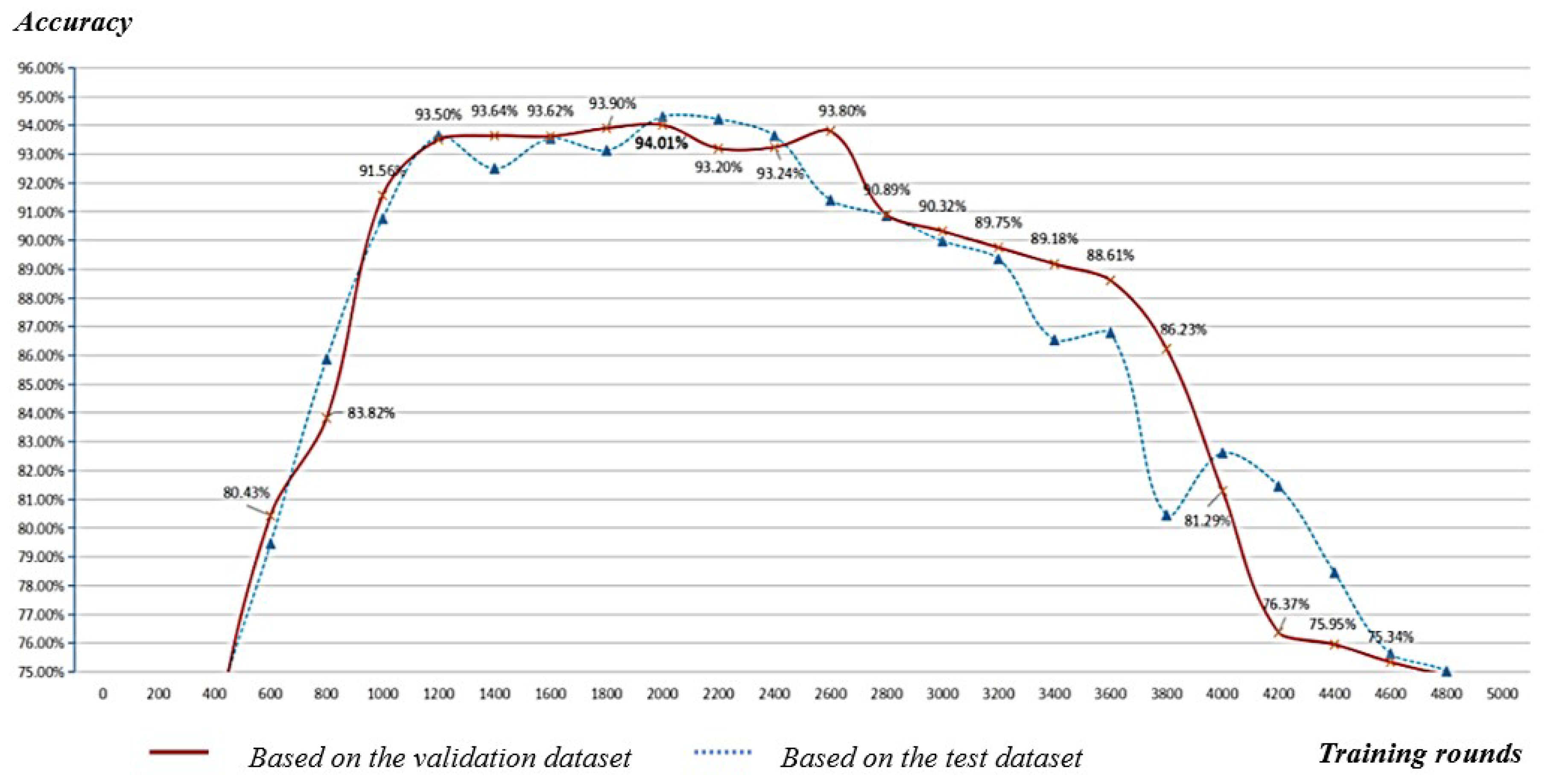
When predicting a large number of output variables with only a small number of input variables, overfitting can occur during the training process of neural networks. Overfitting can cause a decrease in the prediction accuracy of the neural network. Figure 14 shows the curve of training a global stress neural network using BP neural network without setting convergence judgement. The horizontal axis represents the training rounds, and the vertical axis represents the accuracy. The blue curve represents the accuracy verified by the validation set every 200 rounds of training, while the red curve represents the accuracy evaluated by the test set every 200 rounds of training.

It can be observed that: (1) As the number of training rounds increases, the prediction accuracy of the network first rises, then becomes flat, and finally drops sharply, indicating the phenomenon of overfitting. Therefore, it is necessary to design a convergence rule. (2) The consistent performance trends of the validation set and the test set in terms of accuracy demonstrate that the validation set can effectively provide an approximate evaluation of the network’s performance. Therefore, the following convergence rules should be set when training the neural network for obtaining global stress of the connector structure: when the accuracy of the network verified by the validation set decreases by more than 5%, the network should stop training and the previously trained network should be used as the final network (the initial global stress ANN for Connector Structure).

4.7. Uncertainty Analysis of the Initial ANN Based on Simulation

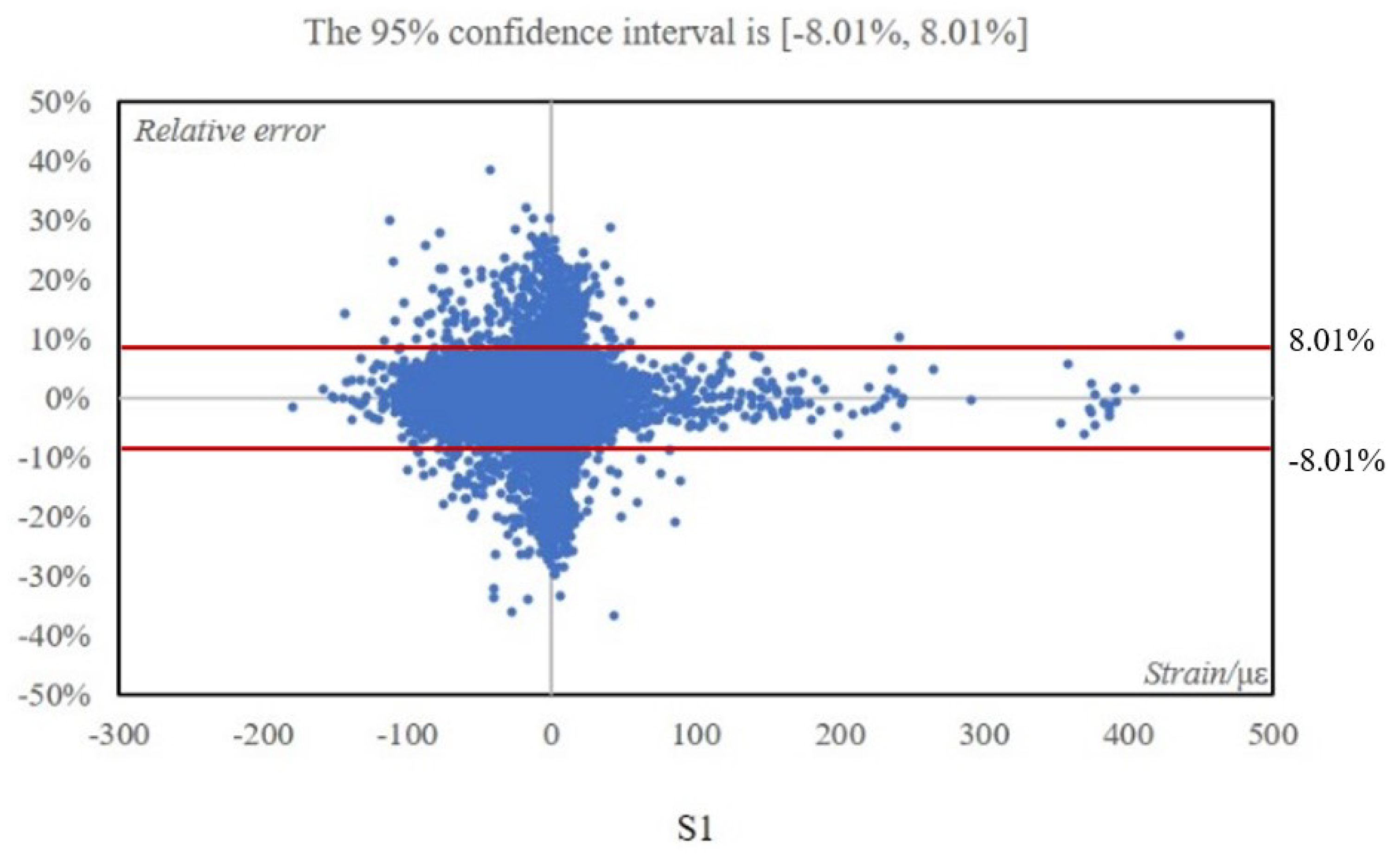
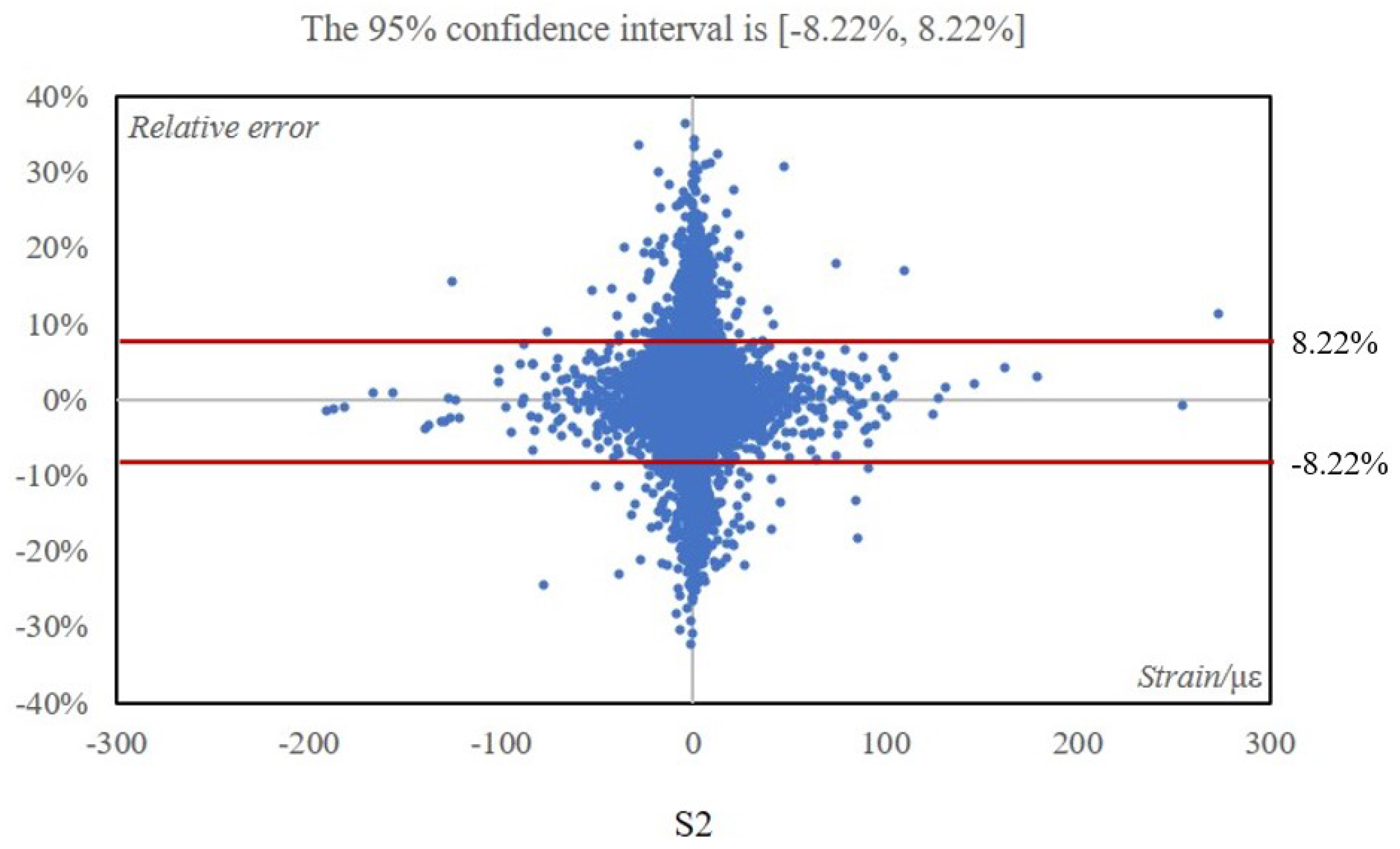
An uncertainty analysis was conducted on the initial ANN for global stress of connectors based on 600 test datasets. Figure 15 and Figure 16 display the relative error distribution of the remaining 30,838 finite elements stress values that were obtained using 20 feature elements’ stress values as inputs, under the working condition of 420 tons of shear force and a direction of 60° (The shear force is considered zero when it’s vertical, and a counter clockwise direction is considered positive). The abscissa denotes the magnitude of strain, and the ordinate represents the relative error. The results show that in the S1 direction, 95% of the finite elements stress values were predicted with an error range of [-8.01%, 8.01%]. Similarly, in the S2 direction, 95% of the finite element stress values were predicted with an error range of [-8.22%, 8.22%] [25].

5. Verify Accuracy by Physical Structure Test

5.1. Physical Test Object

To verify the accuracy of the ANN in obtaining the global stress of the single-ear connector structure, physical structural tests were conducted using a 1:1 model. The main parameters of the single-ear connector model are presented in Table 2.

5.2. Arrangement of the Stress Sensors

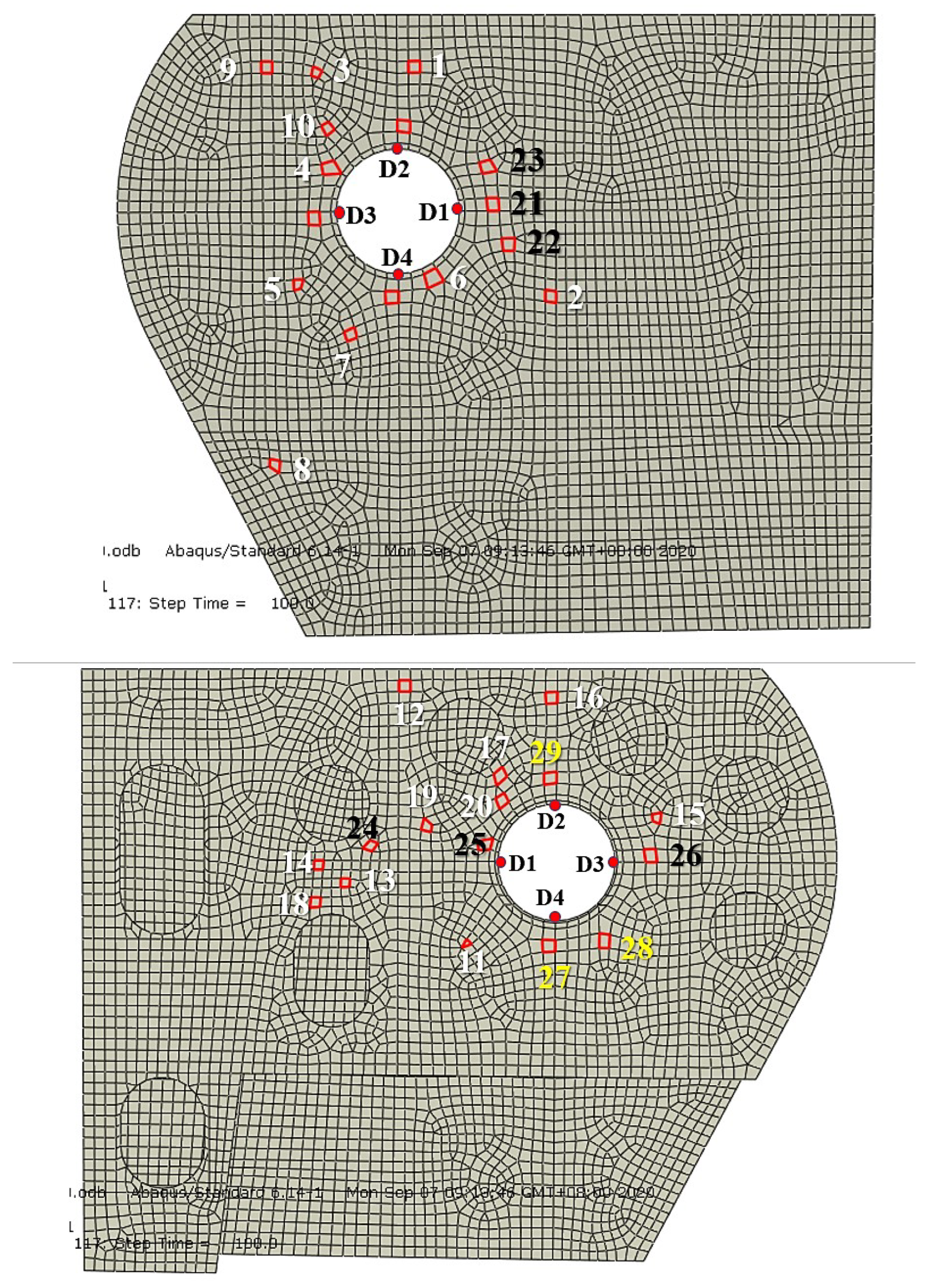
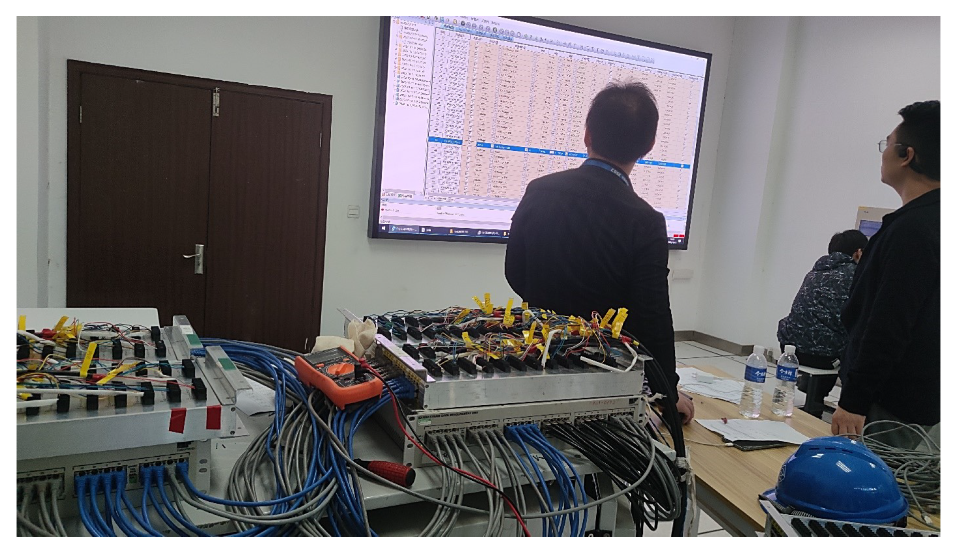
A total of 29 three-dimensional stress measurement points were set up for the test, as shown in Table 3, using static strain gauges and three-dimensional strain sensors, as shown in Figure 17. Among these, 20 measurement points located at feature elements provided input data for the ANN. In addition, 6 measurement points were strategically placed in the high-stress areas of the outer and intermediate bulkheads to fine-tune the ANN. Finally, 3 measurement points were placed in arbitrary positions within the high-stress area to assess the accuracy of the network. The locations of all stress sensors are shown in Figure 18. D1, D2, D3, and D4 are four reference points located at the edge of the connector, which are used to locate the element coordinates.

5.3. Process of the Test

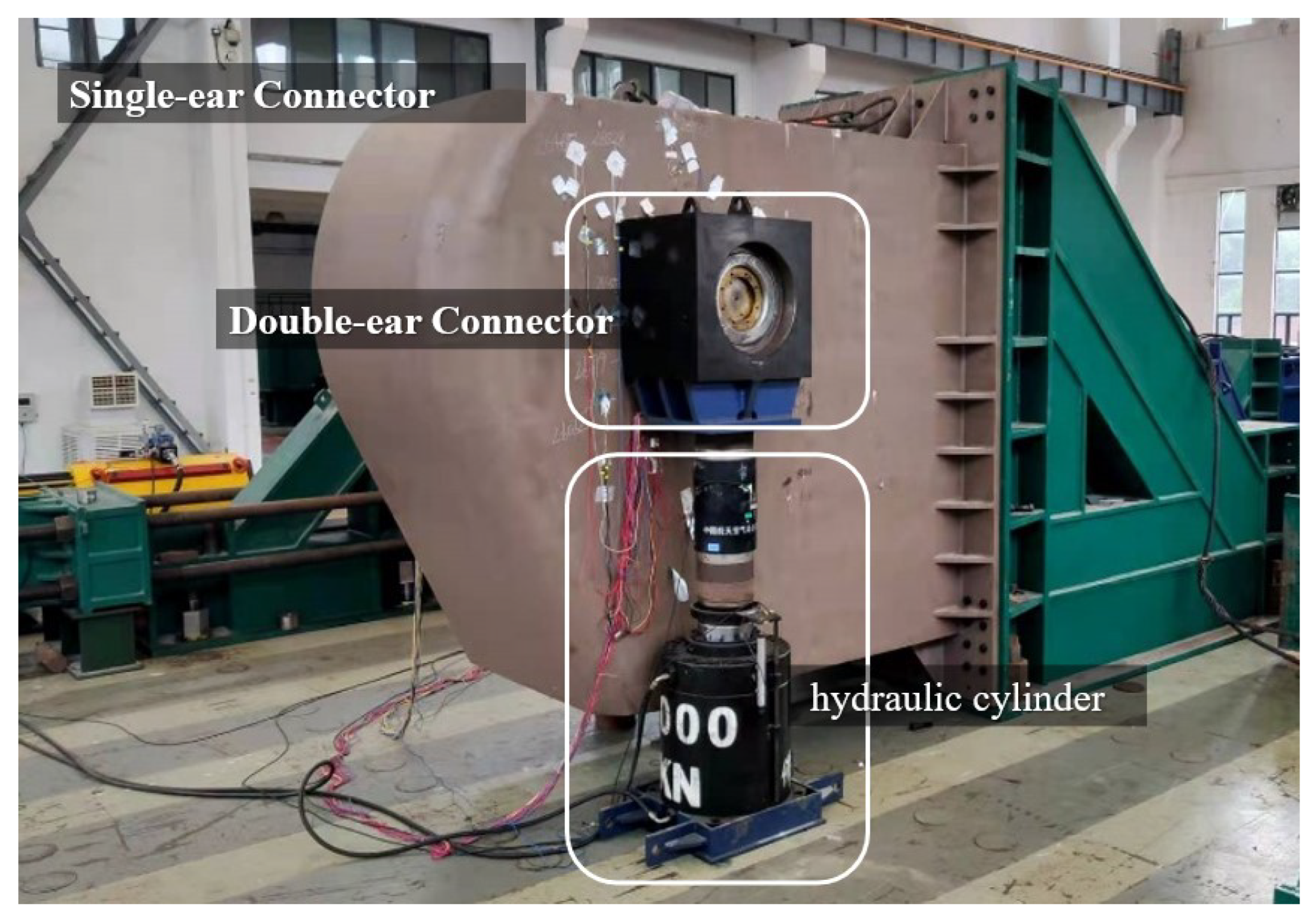
A fixture was utilized to simulate the adjacent double-ear connector, while a hydraulic cylinder was used to apply simulated shear forces. Precise control of the shear force was achieved using a force sensor, with the inclined angle simulated by fixing a bottom block to the cylinder, as shown in Figure 19 and Figure 20. The test was conducted within the elastic ranges, and the loading scheme is presented in Table 4. The loads during the fine-tuning phase did not overlap with those during the accuracy verified phase.

5.4. Test results

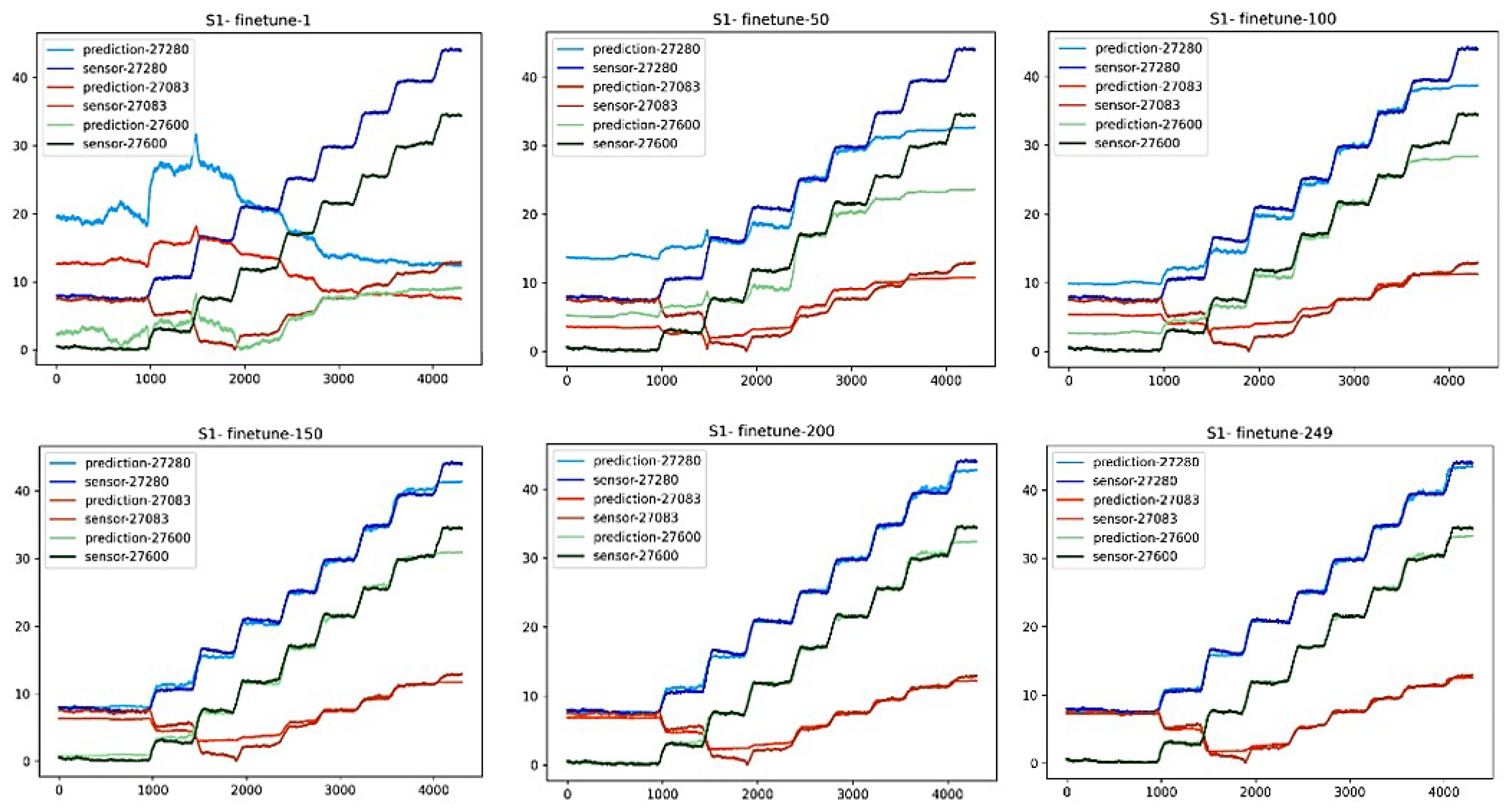
(i) Figure 21 illustrates the process of fine-tuning a neural network at a loading angle of 10 degrees. The horizontal axis represents the experimental time steps, and the vertical axis represents the measured stress values. The neural network predicts the stress data for three randomly selected validation elements, after 249 rounds of fine-tuning, the neural network can accurately predict the stress value.

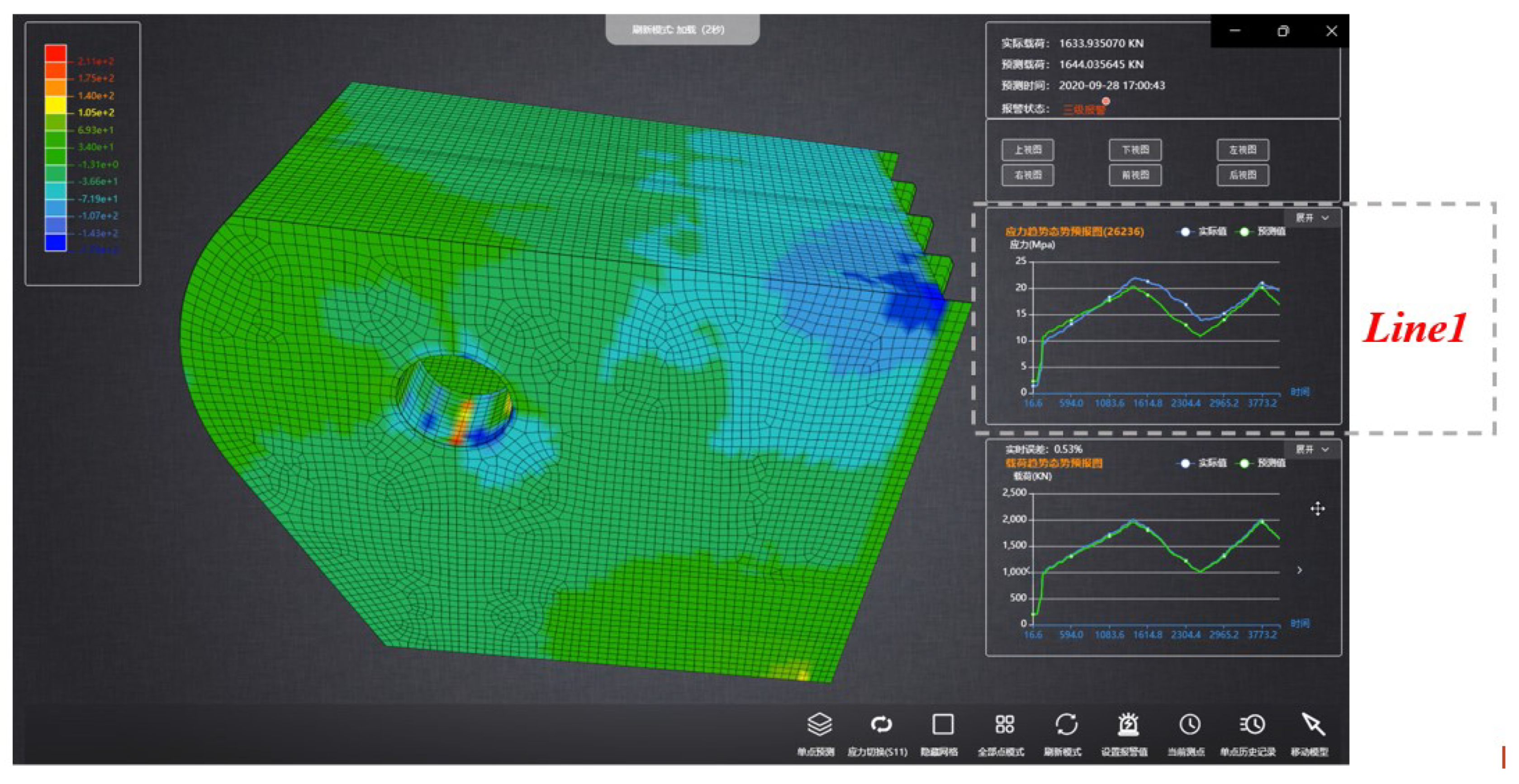
(ii) Based on the fine-tuned neural network, a real-time global stress solver for connector structures was developed and embedded into the Structural Health Monitoring system software, as shown in Figure 22. It shows the stress field contour map obtained by the software under a vertical shear force of 1634 kN. The software can recognize the load direction as vertically upward, and the maximum stress is located under the pinhole of the connector. Both sides and the upper side of the pinhole are also high-stress areas. The farther away from the pinhole, the lower the stress amplitude of the structure.

(iii) Curve 1 is the comparison curve between the measured stress values and the stress values solved by the neural network under the above working condition. The blue curve represents the measured data, and the green curve represents the data predicted by the neural network. The overall solution accuracy is as high as 93.6% by comparison.

6. Conclusion

In summary, this paper proposes an innovative method based on artificial intelligence for real-time solution of stress fields of marine structures using a small number of stress sensors. The method divides the spatial structure into subsets of finite elements with significant correlations between each other, and selects feature elements from each subset as stress measuring points. Then, a neural network is used to establish the relationship between the feature elements and the corresponding subset to reconstruct the global stress of the structure.

Additionally, a neural network optimization network (initial network) is established based on finite element simulation data to assess the safety of the connector structure of a marine platform. The network uses 20 feature elements as input variables and can predict the remaining 30,858 finite element data. The uncertainty analysis shows that the strain solution error of 95% of the finite elements is within 9%.

To fine-tune the initial network and verify the accuracy of the ANN, a physical 1:1 structural network test of the connector is conducted. The results show that the ANN has an accuracy of 93.6% when compared to the validation points. The proposed method demonstrates feasibility and high predictive accuracy and can upgrade the traditional SHM system from “point" monitoring to “field" monitoring.

References

Zhang Tao, Wei Pengyu, Y.Y. Resistance Spot Welding Method for Metal-Based Fiber Bragg Grating Sensors. Trans. Nanjing Univ. Aeronaut. Astronaut. 2015, 289–296.
Foss, G.C.; Haugse, E.D. Using Modal Test Results to Develop Strain to Displacement Transformations. Proceedings of the 13th International Modal Analysis Conference, 1995, Vol. 2460, Society of Photo-Optical Instrumentation Engineers (SPIE) Conference Series, p. 112.
Ko, W.L.; Richards, W.L.; Tran, V.T. Displacement theories for in-flight deformed shape predictions of aerospace structures. Technical report, 2007.
Ko, W.L.; Richards, W.L.; Fleischer, V.T. Applications of Ko displacement theory to the deformed shape predictions of the doubly-tapered Ikhana Wing. Technical report, 2009.
Ko, W.L.; Fleischer, V.T. Extension of Ko straight-beam displacement theory to deformed shape predictions of slender curved structures. Technical report, 2011.
Tessler, A. A variational principle for reconstruction of elastic deformations in shear deformable plates and shells; National Aeronautics and Space Administration, Langley Research Center, 2003.
Tessler, A.; Spangler, J.L. Inverse FEM for full-field reconstruction of elastic deformations in shear deformable plates and shells. 2nd European Workshop on Structural Health Monitoring, 2004.
Tessler, A.; Spangler, J.L. A least-squares variational method for full-field reconstruction of elastic deformations in shear-deformable plates and shells. Comput. Methods Appl. Mech. Eng. 2005, 194, 327–339. [Google Scholar] [CrossRef]
Tessler, A. Structural analysis methods for structural health management of future aerospace vehicles. Key Engineering Materials. Trans Tech Publ 2007, 347, 57–66. [Google Scholar]
Kefal, A.; Mayang, J.B.; Oterkus, E.; Yildiz, M. Three dimensional shape and stress monitoring of bulk carriers based on iFEM methodology. Ocean Engineering 2018, 147, 256–267. [Google Scholar] [CrossRef]
Kefal, A.; Oterkus, E.; Tessler, A.; Spangler, J.L. A quadrilateral inverse-shell element with drilling degrees of freedom for shape sensing and structural health monitoring. Eng. Sci. Technol. Int. J. 2016, 19, 1299–1313. [Google Scholar] [CrossRef]
Ke, Z.; Shenfang, Y.; Yuanqiang, R.; others. Shape reconstruction of self-adaptive morphing wings’ fish bone based on inverse finite element method. Acta Aeronaut. Et Astronaut. Sinaca 2020, 41, 250–260. [Google Scholar]
Oh, B.K.; Park, H.S.; Glisic, B. Prediction of long-term strain in concrete structure using convolutional neural networks, air temperature and time stamp of measurements. Autom. Constr. 2021, 126, 103665. [Google Scholar] [CrossRef]
Ye, X.; Chen, X.; Lei, Y.; Fan, J.; Mei, L. An integrated machine learning algorithm for separating the long-term deflection data of prestressed concrete bridges. Sensors 2018, 18, 4070. [Google Scholar] [CrossRef] [PubMed]
Dai, H.; Zhang, H.; Wang, W. A multiwavelet neural network-based response surface method for structural reliability analysis. Comput. -Aided Civ. Infrastruct. Eng. 2015, 30, 151–162. [Google Scholar] [CrossRef]
Liu, J.H.; Cheng, J.S.; Chen, J.P. Support vector machine training algorithm: A review. Inf. Control-Shenyang- 2001, 31, 45–50. [Google Scholar]
Zhang, T.; Hu, J.; Wang, X.; Chen, G.; Zhu, Q.; Jiang, Z.; Wang, Z. Solving approach for global stress field of the 3D Structures based on artificial intelligence. Ship Mechanics 2023, 27, 238–249. [Google Scholar]
Lu, W.; Peng, Q.; Cui, Y.; Huang, Z.; Teng, J.; Hu, W. Structural response estimation method based on particle swarm optimisation/support vector machine and response correlation characteristics. Measurement 2020, 160, 107810. [Google Scholar] [CrossRef]
Zhang, H.; Ji, B.; Liu, S.; others. Digital twin mechanism model for the structural safety of pipelines in geohazards area. Oil & Gas Storage Transp. 2021, 10, 1099–1104. [Google Scholar]
Cooper, S.B.; DiMaio, D. Static load estimation using artificial neural network: Application on a wing rib. Adv. Eng. Softw. 2018, 125, 113–125. [Google Scholar] [CrossRef]
Tang, M.; Zhang, Z.; Guo, Z.; Ding, J.; Qi, E.; Gu, X. Design and Assessment Approach of Flexible Connectors for a Double-module Semisubmersible Platform near Island and Reef. The 29th International Ocean and Polar Engineering Conference. OnePetro, 2019.
Miao, Y.; Cheng, X.; Ding, J.; Tian, C.; Zhang, Z. Investigation on hydrodynamic performance of a two-module semi-submersible offshore platform. Ships Offshore Struct. 2022, 17, 607–618. [Google Scholar] [CrossRef]
Zhang, H.; Xu, D.; Lu, C.; Qi, E.; Tian, C.; Wu, Y. Connection effect on amplitude death stability of multi-module floating airport. Ocean Engineering 2017, 129, 46–56. [Google Scholar] [CrossRef]
Shi, Q.; Zhang, H.; Xu, D.; Qi, E.; Tian, C.; Ding, J.; Wu, Y.; Lu, Y.; Li, Z. Experimental validation of network modeling method on a three-modular floating platform model. Coastal Engineering 2018, 137, 92–102. [Google Scholar] [CrossRef]
Zhu, Q.; Zhang, T.; Wang, X.; Jiang, Z.; Yue, Y. A model of structural stress reverse deduction and its uncertainty quantitative analysis. Equip. Environ. Eng. 2023, 20, 69–76. [Google Scholar]

Figure 1. Schematic diagram of correlation coefficients and correlation degrees.

Figure 2. Simple neural network to obtain global stress.

Figure 3. Technical path of building initial network.

Figure 4. Fine-tuning process of the initial network.

Figure 5. Connector structure of the offshore platform.

Figure 6. Single ear and double ear connector structure.

Figure 7. Inner bulkhead of connector structure.

Figure 8. Selection process of the feature Finite Elements.

Figure 9. Identifier of the selected 50 feature finite elements.

Figure 10. The count of correlated elements of each feature element (Load sensitivity from strong to weak).

Figure 11. Influence of the number of feature elements on the solution accuracy.

Figure 12. Solution process of the BP neural network.

Figure 13. Solution process of the DNN neural network.

Figure 14. Overfitting curve during the training process of neural networks.

Figure 15. Solution uncertainty for global stress in S1 direction.

Figure 16. Solution uncertainty for global stress in S2 direction.

Figure 17. Static stress testing equipment

Figure 18. The locations of all stress sensors.

Figure 19. The framework of the test.

Figure 20. Several loading conditions during the test.

Figure 21. Fine-tuning process of the ANNs under the loading angle of 10° (The horizontal axis represents time with the unit of second; the vertical axis represents the stress with the unit of MPa).

Figure 22. The stress field contour map obtained by ANNs under a vertical shear force of 1634 kN.

Table 1. Comparison of solution accuracy of different neural networks.

	BP	CNN	RNN	DNN
Minimum accuracy	90.40%	85.30%	90.60%	88.90%
Maximum accuracy	94.70%	88.80%	93.40%	94.80%

Table 2. Main parameters of the connector model

Principal dimension	Length	3.95 m
Principal dimension	Width	1.70 m
Principal dimension	Height	3.20 m
Material	Double-ear connector (the fixture)	42CrMo Steel (yield strength 450 MPa)
Material	Single-ear connector	ZG230-450H Steel (yield strength 240 MPa)

Table 3. Information of all stress sensors.

Sensor No.	Element NO.	Phase	Bulkhead located in	Reference Point	Relative coordinates
1	26234	Training	Outside	D2	(89.84,416.83)
2	25799	Training	Outside	D1	(467.49,-441.92)
3	26528	Training	Outside	D2	(-417.30,387.32)
4	26498	Training	Outside	D3	(-31.06,221.78)
5	26009	Training	Outside	D3	(-203.11,-327.83)
6	25834	Training	Outside	D4	(179.59,-22.26)
7	26084	Training	Outside	D4	(-251.62,-312.10)
8	25507	Training	Outside	D4	(-654.56,-983.12)
9	26465	Training	Outside	D3	(-352.14,734.94)
10	26631	Training	Outside	D3	(-40.61,425.31)
11	27158	Training	Inside	D1	(143.40,-431.74)
12	27645	Training	Inside	D1	(474.93,911.95)
13	27943	Training	Inside	D1	(783.21,-116.72)
14	27844	Training	Inside	D1	(924.08,-23.91)
15	27572	Training	Inside	D3	(-199.49,229.65)
16	27662	Training	Inside	D2	(30.09,530.90)
17	27765	Training	Inside	D2	(295.11,126.20)
18	27988	Training	Inside	D1	(957.63,-42.27)
19	27738	Training	Inside	D1	(354.69,181.96)
20	27754	Training	Inside	D1	(-36.55,317.18)
21	26254	Fine-tuning	Outside	D1	(175.36,33.17)
22	25753	Fine-tuning	Outside	D1	(255.65,-173.21)
23	26299	Fine-tuning	Outside	D1	(145.95,226.70)
24	28090	Fine-tuning	Inside	D1	(649.69,78.04)
25	27672	Fine-tuning	Inside	D1	(51.76,85.79)
26	27490	Fine-tuning	Inside	D3	(-170.9,34.2)
27	27280	Verified	Inside	D4	(33.2,-120.4)
28	27083	Verified	Inside	D3	(64.01,-412.54)
29	27600	Verified	Inside	D2	(33,115.75)

Table 4. Detailed loading conditions.

Phase	Force (kN)	Cycle times
Fine-tuning	1000,1100,1200,1300,...,2000,1900,...,1000	3
Accuracy verified	2000,2100,2200,2300,2400,2500	1

Disclaimer/Publisher’s Note: The statements, opinions and data contained in all publications are solely those of the individual author(s) and contributor(s) and not of MDPI and/or the editor(s). MDPI and/or the editor(s) disclaim responsibility for any injury to people or property resulting from any ideas, methods, instructions or products referred to in the content.

© 2023 by the authors. Licensee MDPI, Basel, Switzerland. This article is an open access article distributed under the terms and conditions of the Creative Commons Attribution (CC BY) license (http://creativecommons.org/licenses/by/4.0/).

Copyright: This open access article is published under a Creative Commons CC BY 4.0 license, which permit the free download, distribution, and reuse, provided that the author and preprint are cited in any reuse.

MDPI Initiatives

Important Links

Choose an area of interest and we will send you notifications of new preprints at your preferred frequency.

Disclaimer

Reconstructing the Global Stress of Marine Structures Based on Artificial Intelligence

Abstract

1. Introduction

2. Correlation Analysis Among FE of Marine Structure

2.1. Correlation Between the Finite Elements

2.2. Correlation Analysis Method

3. Neural Networks Architecture Method

3.1. Principles of Neural Networks

3.2. Initial ANN for Global Stress

3.3. Fine-tuning of Initial Network

4. Reconstructing Global Stress for Connector Structure

4.1. Mechanical Analysis on the Connector Structure

4.2. Data samples

4.3. Selecting Feature Elements by Correlation Analysis

4.4. Optimization of the Number of Stress Sensors

4.5. Optimization of neural networks

4.6. Convergence of Neural Network

4.7. Uncertainty Analysis of the Initial ANN Based on Simulation

5. Verify Accuracy by Physical Structure Test

5.1. Physical Test Object

5.2. Arrangement of the Stress Sensors

5.3. Process of the Test

5.4. Test results

6. Conclusion

References

MDPI Initiatives

Important Links

Subscribe