
Submitted:
30 May 2023
Posted:
30 May 2023
You are already at the latest version
Abstract
Driven by the rapidly growing demand for information security, covert wireless communication conceived as one of the essential technology has attracted tremendous attention. However, traditional wireless covert communication is continuously exposing the inherent limitations that challenge deploying in environments with a large number of obstacles, such as cities with high-rise buildings. In this paper, we propose an intelligent reflecting surface (IRS) assisted covert communication system (CCS) with a friendly UAV, where the UAV generates artificial noise (AN) to interfere with the monitors. Furthermore, we model the power of AN emitted by UAV as an uncertainty model, with which the closed-form detection error probability (DEP) on the covert wireless communication for the monitor is derived. Under the derived DEP, we formulate the optimization problem to maximize the covert rate, and an iterative algorithm is designed to solve the optimization problem to obtain the optimal covert rate by using Dinkelbach method. Simulation results show that the proposed system achieves the maximum covert rate when the phase of the IRS units, the trajectory, and the transmit power of the UAV are jointly optimized.
Keywords:
information security
; covert communication
; intelligent reflectors surface
; UAV
1. Introduction
Traditional cryptography mechanisms protect sensitive data with the encryption of messages into cipher text, preventing access by unauthenticated users[1]. However, these cipher texts generated with cryptography mechanisms exhibit a high degree of randomization, which can easily arouse the suspicion of adversaries [2,3]. In this case, more powerful decryption methods and mechanisms may be employed to crack randomized data streams, which severely threaten the security of the information protected by the cryptography regime [4,5]. In this scenario, covert communication, which can be used to transmit sensitive information without being perceived, attracts tremendous attention [6].
In general, a transmitter can use covert communication to transmit sensitive data to legal receivers without the communication process being detected by malicious adversaries. In covert communication systems, covert information can be carried by normal messages and transmitted together with these normal messages to avoid being perceived by adversaries [7]. However, the small capacity with a high bit error rate (BER) limits the application of the traditional covert communication systems (CCS) [8]. To improve the efficiency and reliability of wireless CCSs, the intelligent reflecting surface (IRS) has been introduced into CCS [9]. IRS, also known as reconfigurable intelligent surface, is a low-cost technology that integrates a large number of passive reflecting units to intelligently adjust the reflected phase shift of signals in the environment [10]. Recently, IRS has been gradually applied to wireless CCS to improve its performance. Initially, an IRS-based method is proposed to take advantage of the smartly controlled surface to modify unforeseen propagation conditions that could reveal messages[11]. Furthermore, the authors of [12] proposed an IRS-aided CCS system, and the data rate, the transmit power, and the reflection matrix of IRS are jointly optimized. To reduce the computational complexity, a low-complexity penalty-based successive convex approximation (SCA) algorithm was proposed to jointly optimize the communication schedule and the reflection matrix of IRS [13]. Besides, the IRS-aided CCS with multiple input multiple output (MIMO) has been proposed in [14,15], where the high coupling is exploited for alternative optimization to find the optimal solution. Similarly, non-orthogonal multiple access methods are adopted in [16,17] to design the IRS-assisted CCS, which exploits the phase-shift uncertainty of the IRS as the cover medium to hide the existence of covert transmission. And a passive IRS-assisted CCS was proposed in [18] to adjust the phase shifts of the IRS to align the phases of the received reflected signals and meanwhile to adjust the reflection amplitude to satisfy the covert constraint. However, the covert information in IRS-assisted wireless CCS is vulnerable to adversaries.
To improve the security of wireless CCS, friendly nodes are utilized to jam adversaries [19,20]. Due to being able to be fast deployed with flexible configuration and the presence of short-range line-of-sight links[21], UAVs frequently perform as friendly nodes. For CCS, when the locations of the legal users and the monitors can not be determined, the UAV can perform as a relaying node to deliver messages between the legal users covertly to avoid detection by the monitors. As a pioneer work, a UAV-aided CCS is designed in [22], where the UAV trajectory and transmit power for the UAV are alternately optimized to maximize the average covert rate. Based on this, Xu proposed a model for UAV-assisted CCS with multiple users [23]. Furthermore, to cope with the complex communication environment, a UAV with multiple antennas is designed in [24] to jam the monitor in the CCS, which can count the multiple monitors colluding to listen to adjacent users. Similarly, Du proposed a multi-antenna UAV to assist the covert communication system with a power allocation algorithm, which can be used to avoid detection from the monitor with multiple antennas [25]. Owing to the substantial enhancement in performance obtained by UAV and IRS, numerous frameworks incorporating UAV and IRS have been proposed [26,27,28]. However, how to effectively use UAVs with IRS to design an efficient wireless covert communication system is still challenging.
In this paper, we propose an IRS-assisted covert communication system with a friendly UAV, where the UAV can be utilized to reinforce message security and the IRS can be employed to improve the covert rate. Moreover, thanks to the high mobility of UAVs, the proposed CCS can be deployed in complex communication environments with various communication barriers, which improves reliability. The contributions of this paper are listed as follows:
- We propose an IRS-assisted covert communication system, where a UAV performs as the jammer to interfere with the monitor to reduce the detection rate.
- We derive the minimum detection error probability (DEP) for the monitor by modeling the artificial noise (AN) power at the UAV as an uncertainty model under the assumption that the coordinates of the UAV and the transmitter are available.
- We formulate the optimization problem to maximize the covert rate for the covert communication system by optimizing the trajectory and the transmit power of the UAV. Furthermore, we develop the iterative algorithm by using SCA and Dinkelbach methods to solve the optimization problem.
The rest of this paper is organized as follows. Section 2 describes the system model. Section 3 formulates the optimization method considering the target of maximizing the covert rate at Bob. Section 4 presents the optimal algorithm to solve the problem described in Section 3. Section 5 displays the simulation results of the algorithm. Finally, Section 6 concludes this paper.
2. System Model
Figure 1 demonstrates an IRS-assisted CCS, where there are a transmitter and a receiver of covert messages, and a monitor. The transmitter of covert messages, which generally is a base station, is denoted as Alice in common CCSs, and the receiver is denoted as Bob. The monitor denoted as Willie keeps on observing the communication between Alice and Bob to determine whether there is a covert communication channel between Alice and Bob. Since there exists a large volume of barriers in communication surroundings, such as cities with large buildings, the links between Alice and Bob and Alice and Willie are not a line of sight (LoS). In this case, we propose to deploy IRS on the surface of the buildings to relay messages from Alice to Bob. However, if Willie locates close to Bob, the received signal power of Willie increases with that of Bob when adopting the IRS, which enlarges the probability of Willie detecting covert communication between Alice and Bob. Thus, we adopt a UAV as a friendly node for Alice to interfere with Willie’s to detect the covert communication between Alice and Bob.
The fading of the channels are respectively denoted as (Alice and IRS), (IRS and Bob) and (IRS and Willie). Let all nodes be in a three-dimensional Cartesian coordinate system, and Alice, IRS, Bob, and Willie be in the ground plane with a height of 0. Thus, their coordinates can be expressed as , , , and , respectively. Moreover, We assume that the positions of Alice, IRS, UAV, Bob, and Willie are known to each other. Let the start and end coordinates of the UAV be and respectively, and thus the UAV flies from the start coordinate to the coordinate in finite time N, where and L is the length of a single time slot, allowing N to be divided into T intervals.
Define as the set of UAV coordinates. Let , and we have
where represents the position of the UAV in t-th time slot, , and is the maximum speed of the UAV.
In addition, the IRS consists of M reflecting elements. The phase shift and amplitude of the IRS in t-th time slot are defined as a matrix , where . When the optimal amplitude is obtained, can be set as 1, then the diagonal matrix can be rewritten as .
2.1. Channel Model
In a practical system, due to the high altitude of the UAV, the UAV-to-ground communications can be treated as line-of-sight (LOS) links. Therefore, we model the UAV-to-ground communication channel as a free-space path loss model, where the signal can propagate along a straight line without obstacles between the transmitter and the receiver. In this scenario, the gain of the channel between UAV and Bob can be described as
Similarly, the channel gain between UAV and Willie is
where is the channel power gain over the channel at distance . The channel between Alice, Bob, and Willie is considered a non-line-of-sight (NLOS) channel due to the blockage of the obstacles. Consider the IRS as a uniform linear array (ULA) antenna, i.e., a system of antennas arranged in a plane according to a linear law called an antenna array. Then the gain of the channel from Alice and IRS is
where denotes the path loss, is the distance between Alice and IRS, is the cosine of the AoA of the signal from the UAV to the IRS in t-th time slot, and d is the antenna distance and is the carrier wavelength.
Similarly, the channels from IRS to Bob and Willie are considered LOS channels, and thus the fading of the channels between IRS and Bob and Willie can be expressed as
where is the distance between IRS and Bob, is the distance between IRS and Willie, and and are the cosines of the angle of departure (AoD) of the signals that Bob and Willie received from the IRS, respectively.
Assuming that the channel utilization tends to be maximum in each time slot, according to (3), (4), and (5), the received signal of Bob is
where is the transmit power of Alice, is the signal sent by Alice in t-th time slot, which follows a complex Gaussian distribution with mean 0 and variance 1, i.e., . is the AN signal transmitted by the UAV that satisfies , is the AWGN with mean 0 and variance at Bob, i.e., , and is the AN transmit power of the UAV, and follows a uniform distribution over the interval , where is the maximum AN transmit power of the UAV, taking values in the range .
Accordingly, the Probability Density Function (PDF) is expressed as
According to (7), the receiving rate of Bob is
2.2. Detection on CCS by Willie
In this subsection, Willie determines the presence of covert communications by analyzing the received signals. To detect covert communications, Willie employs the hypothesis testing method. Willie first perceives the location of Alice, UAV, and IRS, and then according to (3), (4), and (6), the received signal at Willie can be obtained as
where denotes that there is no covert message transmitted between the UAV and Bob, indicates the opposite, and is the additive white Gaussian noise (AWGN) with mean 0 and variance at Willie, i.e., . Since the data rate tends to be the same in each time slot, the received power at Willie can be expressed as
Assume that Willie employs a radiometer detector in each time slot to detect transmissions from Alice to Bob.
Consider to be Willie’s detection threshold. If , the decision state is , indicating that Willie determines that there exist covert communications between UAV and Bob. Otherwise, the decision state is , which indicates that Willie determines there is no covert message being transmitted. Thus, Willie’s decision rule can be denoted by
3. System Optimization
In this section, we first derive the false alarm probability (FAP) and the missed detection probability (MDP) of Willie, and then the closed-form detection error probability (DEP) is also derived. Under the constraint that the derived DEP of Willie is optimal, we formulate the optimization problem to maximize the covert rate.
3.1. Optimal DEP of Willie
To optimize the DEP of Willie, we first present the definition of FAP and MDP. On one hand, the FAP is the probability that a covert communication between Alice and Bob does not exist, while Willie determines that there is a covert communication, denoted as . According to (11), we have
On the other hand, the MDP is the probability that Willie determines that there is no covert message transmitted from Alice to Bob while there exist covert communications, denoted as . According to (12), we have
According to (13) and (14), the DEP for Willie to detect the covert communication between Alice and Bob is
where , and is the specific value for determining the required covertness.
To optimize DEP, we define a detection threshold as that corresponds to an optimal detection error rate . Then, the DEP of Willie can be expressed as
Note that , since the UAV is used to interfere with Willie. According to (15), when and , an error is detected for . Therefore, these two cases are not considered by Willie. When ,
Similarly, When ,
According to (15), (19), and (20), when , is monotone declining with regard to . When , c is a constant.
If , is monotone increasing with regard to . As a result, is firstly decreasing and then increasing for . If the detection threshold ranges in , the corresponding best detection error rate can be obtained, expressed as
3.2. Reliability of CCS
As the UAV interferes with Willie in receiving signals, Bob is also interfered with, which may reduce the covert rate and impose influence on the reliability of the CCS. According to (9), the outage probability of the covert channel between Alice and Bob can be given by
where is the transmission rate of Bob.
Given the upper bound on the outage probability as , i.e., when the outage probability satisfies , the reliability of the covert channel between Bob and Alice can be guaranteed. From (22), is monotone increasing with regard to . Thus, as the covert rate achieved its maximum value, the outage probability reaches its upper limit . Then, the maximum covert rate is given by
To ensure covertness, the UAV is used to jam Willie and maximize the average received rate of Bob. Therefore, the maximization of the covert rate can be formulated as a joint optimization problem of the UAV trajectory, the IRS phase shift, the transmit power at Alice, and the transmit power of the UAV. According to (21) and (22), this optimization problem can be expressed as
where , . (24a) is a linear objective function, and () and () are mobility constraints of the UAV with convexity. However, (24b) is non-convex about C and , which results in this optimization problem not being solved efficiently.
4. Optimization Algorithm
To solve (Section 3.2), we decompose it into two separate issues, namely the optimization of the Alice transmission power and the AN power of the UAV, and the trajectory of the UAV. For this purpose, the phase of the received signal is first used to obtain the maximum transmission rate, and then the optimal phase shift of the IRS can be obtained. Then, (Section 3.2) is transformed into a trajectory optimization problem for the UAV. Finally, we formulate the optimal trajectory optimization problem with the SCA method.
4.1. Phase Shift Optimization for IRS
To optimize the phase shift of the IRS, in (23) can be expressed as
Then, Bob combines the signals transmitted from different paths via IRS, and the received power of the combined signals can be increased in order to improve the covert rate. The phase shift of the IRS can then be expressed as
where is the direction to be aligned. Thus, the cell phase shift of the m-th IRS can be expressed as
For simplicity, substitute (27) into (25), and the maximum value can be approximated by deriving the upper bound on with
Then, with phase alignment, we can obtain the best .
4.2. Power Optimization
Given C, the optimization problem formulated in (Section 3.2) can be rewritten as
where (29a) and (29b) are non-convex functions and can not be easily solvable. To solve the problem, in (29a) can be re-expressed as
According to Dinkelbach theory, (30) can be transformed into a linear function with an equation factor as
The initial value of is obtained by choosing the small maximum values for and .
According to (21), () can be equivalently expressed as
4.3. Trajectory of UAV Optimization
Given P and , the alternative for (Section 3.2) is
where , (34a) and (34b) are non convex. According to (21), (29b) can be rewritten as
The right side of (35) is a constant with all known variables. And the left side of (35) includes the variables to be optimized. The distance between UAV and Bob (or Willie) can be expressed as , where and . For , we have
The first-order partial derivatives of with respect to and are respectively expressed as
and
Due to and , the Hessian matrix is a positive definite matrix, which means is a convex function. The left side of the inequality in (35) is consequently a convex function, and thus (34b) can be replaced by a convex function. For (34a), we relax the objective function by introducing relaxation variables and . Therefore, (Section 4.3) is rewritten as
where . () is a non-convex function while the left side of () is convex, such that we can obtain a global lower bound estimate for the original function using a first-order Taylor expansion of the convex function. We conduct the Talor expansion of at , and we have
In this manner, the objective function and constraints of the problem (Section 4.3) are both convex. Thus, (44) is convex and can be solved by using the CVX solver to obtain the optimal flight trajectory of the UAV.
4.4. Optimization Algorithm
In this subsection, we develop an iterative optimization algorithm based on SCA and Dinkelbach to solve the problem (Section 3.2), as presented in Algorithm 1.
| Algorithm 1 Iterative Optimization Algorithm based on Dinkelbach |
|
As shown in Algorithm 1, the initial trajectory set and coordinate set of UAV are set up first, then calculating and setting the iteration parameter k. The optimal is calculated with (26). From lines 3 to 9, we design an iterative loop. First, is updated by solving the problem (Section 4.2) with CVX. Second, the factor is updated via (31), and the can be updated by solving (Section 4.3). Finally, the is updated through (24a). The loop terminates when the condition is satisfied. The algorithm returns the optimal UAV AN power , optimal transmission power P, the optimal trajectory of UAV Q, and the maximum average covert rate received at Bob .
5. Numerical Results
In this section, we present the numerical results for the IRS-assisted CCS with UAVs. Furthermore, Algorithm 1 is designed based on SCA and Dinkelbach to solve the formulated optimization problem. The parameters are listed in Table 1.
Figure 2 shows the trajectory comparison of the UAV that works as a jammer to assist the CCS. The initial trajectory, denoted as , represents the UAV moves with uniform speed from the initial point to the endpoint without optimization. From the trajectory optimized by the proposed algorithm, we can observe that the UAV starts from the initial point, and then flies at the maximum speed to Willie in the shortest path. when approaching Willie, the UAV hovers around closer to Willie than Bob. Finally, the UAV travels to the endpoint at the maximum speed in the shortest distance. We can observe the transmit power of Alice and the AN power of the UAV are adjusted simultaneously to guarantee the maximum covert rate. In addition, due to the limit on AN power, the UAV achieves a higher covert rate by approaching Willie, which can ensure covertness for the CCS. Furthermore, if the UAV is close to the initial point, Alice reduces the transmit power and the UAV enlarges the AN power to guarantee covertness, which leads to a small covert rate. In this case, the UAV flies close to Willie at a maximum speed.
Figure 3 displays the covert rate versus flying time with different UAV altitudes and different numbers of IRS units. The IRS is divided into 30 and 40 units, and the UAV flying times are chosen as 30s, 50s, 70s, 90s, 110s, and 130s, respectively. Add to that, the UAV altitude is 50m and 75m.
From Figure 3, we can first observe that the average covert rate increases with flying time. As the flying time increases the UAV spends a longer percentage of its time to jam Willie on receiving signals. Therefore, increasing the flying time will improve transmission efficiency. Second, as the IRS unit increases, the corresponding average transmission rate increases. The reason is that the IRS can intelligently adjust the reflection of the signals to the best direction to achieve a high covert rate. Third, the average covert rate decreases with the height of the UAV. The reason is the fact that the increasing altitude results in a large distance between the UAV and Willie, which brings more path loss for the interfering signal. In this case, Alice reduces the transmission power to ensure the covertness of the covert communication, which leads to a lower covert rate.
To evaluate the convergence of the proposed algorithm, Figure 4 plots the average covert rate versus iterations for different outage probabilities and the maximum speed of the UAV. The outage probability is set as 0.05, 0.1, and 0.3, and the maximum speed of the UAV is set as 50m/s and 70m/s, respectively. We can observe that a high average transmission rate can be obtained with an increase in outage probability. In addition, when the speed of the UAV increases, the average transmission rate also increases accordingly. This is because as the speed of the UAV increases, the time for UAV to arrive at the optimal jamming coordinate reduces. Thus, the UAV can jam communications of Willie for a long time at the optimal jamming coordinate, which results in an improvement of the covert rate. In this way, increasing both the upper limit of outage probability and the speed of the UAV elevate the covert rate of the proposed CCS.
Figure 5 illustrates the covert rate versus for different noise variances at Willie and noise variance at Bob The noise variance at Willie is respectively set as -120dBm, -100dBm, and -80dBm, and the noise variance at Bob is respectively set as -120dBm and -80dBm. First, We can observe that as grows, the average covert rate increases, which is because is comparatively smaller which means the covertness constraint is relatively loose, leading to a higher average covert rate. For ranges 0 and 0.2, the average covert rate is significantly influenced by , and when is larger than 0.2, the average covert rate is negligibly changed. This is because when the value of is large, the covertness constraint is relatively loose and the average rate can reach its maximum value. Moreover, there is an increase in the covert rate as the noise variance at Willie becomes larger. This is because the interference imposed on Willie increases can help Alice to enlarge the transmit power and increase the covert rate. However, when the noise at Bob increases, the received signals at Bob are influenced and reduce the outage probability.
Figure 6 plots the average covert rate versus the transmit power at Alice with different flying times, which are set as the 30s, 70s, and 110s. The maximum power of AN is set to 1W and 2W, respectively. We observed that the average covert rate increases with the flying time of the UAV, and thus the transmit power is also determined by the flying time of the UAV Therefore, a larger transmit power results in a significant improvement in the covert rate. A higher AN power can not only ensure better covertness but also results in correspondingly higher energy consumption.
6. Conclusions
In this paper, we have proposed an IRS-assisted covert communication system with a friendly UAV deployed in complex environments with communication barriers. The closed form of the DEP of covert communication for Willie is derived by considering Willie’s uncertainty about the transmit power. To maximize the covert rate, we have formulated the joint optimization problem by adjusting the jamming power of the UAV and the transmitting power of the transmitter, where the optimal DEP of Willie, the transmit power of the transmitter, and the transmit power of the AN are established as the constraints. An iterative algorithm based on Dinkelbach is designed to solve the established optimization problem. Simulation results demonstrate that the covertness and covert rate of the system can be improved by increasing the number of IRS, UAV flying time, and interference power.
Funding
This work is supported by the National Key Research and Development Program of China (2020YFB2104200).
References
- Talbot, J.; Welsh, D.; Welsh, D.J.A. Complexity and cryptography: an introduction; Cambridge University Press, 2006; Volume 13. [Google Scholar]
- Cao, H.; Zhu, P.; Lu, X.; Gurtov, A. A layered encryption mechanism for networked critical infrastructures. IEEE Network 2013, 27, 12–18. [Google Scholar]
- Chen, L.; Qiu, L.; Li, K.C.; Shi, W.; Zhang, N. DMRS: an efficient dynamic multi-keyword ranked search over encrypted cloud data. Soft Computing 2017, 21, 4829–4841. [Google Scholar] [CrossRef]
- Penzhorn, W. Fast decryption algorithms for the RSA cryptosystem. 2004 IEEE Africon. In Proceedings of the 7th Africon Conference in Africa (IEEE Cat. No.04CH37590), 2004, Vol. 1, pp. 361–364 Vol.1.
- Zhang, L.; Tan, C.; Yu, F. Fast Decryption of Excel Document Encrypted by RC4 Algorithm. 2020 IEEE 20th International Conference on Communication Technology (ICCT), 2020, pp. 1572–1576.
- Lu, K.; Liu, H.; Zeng, L.; Wang, J.; Zhang, Z.; An, J. Applications and prospects of artificial intelligence in covert satellite communication: a review. Science China Information Sciences 2023, 66, 1869–1919. [Google Scholar] [CrossRef]
- Xiang, W.; Wang, J.; Xiao, S.; Tang, W. Achieving Constant Rate Covert Communication via Multiple Antennas. In Proceedings of the 2022 IEEE 95th Vehicular Technology Conference: (VTC2022-Spring), 2022, pp. 1–6.
- Bash, B.A.; Goeckel, D.; Towsley, D. Limits of Reliable Communication with Low Probability of Detection on AWGN Channels. IEEE Journal on Selected Areas in Communications 2013, 31, 1921–1930. [Google Scholar] [CrossRef]
- Zou, L.; Zhang, D.; Cui, M.; Zhang, G.; Wu, Q. IRS-assisted covert communication with eavesdropper’s channel and noise information uncertainties. Physical Communication 2022, 53, 101662. [Google Scholar] [CrossRef]
- Özdogan, Ö.; Björnson, E.; Larsson, E.G. Intelligent Reflecting Surfaces: Physics, Propagation, and Pathloss Modeling. IEEE Wireless Communications Letters 2020, 9, 581–585. [Google Scholar] [CrossRef]
- Lu, X.; Hossain, E.; Shafique, T.; Feng, S.; Jiang, H.; Niyato, D. Intelligent Reflecting Surface Enabled Covert Communications in Wireless Networks. IEEE Network 2020, 34, 148–155. [Google Scholar] [CrossRef]
- Kong, J.; Dagefus, F.T.; Choi, J.; Spasojevic, P. Intelligent Reflecting Surface Assisted Covert Communication With Transmission Probability Optimization. IEEE Wireless Communications Letters 2021, 10, 1825–1829. [Google Scholar] [CrossRef]
- Song, X.; Zhao, Y.; Wu, Z.; Yang, Z.; Tang, J. Joint Trajectory and Communication Design for IRS-Assisted UAV Networks. IEEE Wireless Communications Letters 2022, 11, 1538–1542. [Google Scholar] [CrossRef]
- Dong, L.; Wang, H.M. Secure MIMO Transmission via Intelligent Reflecting Surface. IEEE Wireless Communications Letters 2020, 9, 787–790. [Google Scholar] [CrossRef]
- Chen, X.; Zheng, T.X.; Dong, L.; Lin, M.; Yuan, J. Enhancing MIMO Covert Communications via Intelligent Reflecting Surface. IEEE Wireless Communications Letters 2022, 11, 33–37. [Google Scholar] [CrossRef]
- Lv, L.; Wu, Q.; Li, Z.; Ding, Z.; Al-Dhahir, N.; Chen, J. Achieving Covert Communication by IRS-NOMA. In Proceedings of the 2021 IEEE/CIC International Conference on Communications in China (ICCC), 2021, pp. 421–426.
- Lv, L.; Wu, Q.; Li, Z.; Ding, Z.; Al-Dhahir, N.; Chen, J. Covert Communication in Intelligent Reflecting Surface-Assisted NOMA Systems: Design, Analysis, and Optimization. IEEE Transactions on Wireless Communications 2022, 21, 1735–1750. [Google Scholar] [CrossRef]
- Wu, Y.; Wang, S.; Luo, J.; Chen, W. Passive Covert Communications Based on Reconfigurable Intelligent Surface. IEEE Wireless Communications Letters 2022, 11, 2445–2449. [Google Scholar] [CrossRef]
- Zhang, R.; Chen, X.; Liu, M.; Zhao, N.; Wang, X.; Nallanathan, A. UAV Relay Assisted Cooperative Jamming for Covert Communications Over Rician Fading. IEEE Transactions on Vehicular Technology 2022, 71, 7936–7941. [Google Scholar] [CrossRef]
- Jiang, X.; Chen, X.; Tang, J.; Zhao, N.; Zhang, X.Y.; Niyato, D.; Wong, K.K. Covert Communication in UAV-Assisted Air-Ground Networks. IEEE Wireless Communications 2021, 28, 190–197. [Google Scholar] [CrossRef]
- Zeng, Y.; Zhang, R.; Lim, T.J. Wireless communications with unmanned aerial vehicles: opportunities and challenges. IEEE Communications Magazine 2016, 54, 36–42. [Google Scholar] [CrossRef]
- Zhou, X.; Yan, S.; Hu, J.; Sun, J.; Li, J.; Shu, F. Joint Optimization of a UAV’s Trajectory and Transmit Power for Covert Communications. IEEE Transactions on Signal Processing 2019, 67, 4276–4290. [Google Scholar] [CrossRef]
- Jiang, X.; Yang, Z.; Zhao, N.; Chen, Y.; Ding, Z.; Wang, X. Resource Allocation and Trajectory Optimization for UAV-Enabled Multi-User Covert Communications. IEEE Transactions on Vehicular Technology 2021, 70, 1989–1994. [Google Scholar] [CrossRef]
- Chen, X.; Chang, Z.; Tang, J.; Zhao, N.; Niyato, D. UAV-Aided Multi-Antenna Covert Communication Against Multiple Wardens. ICC 2021 - IEEE International Conference on Communications, 2021, pp. 1–6.
- Du, H.; Niyato, D.; Xie, Y.a.; Cheng, Y.; Kang, J.; Kim, D.I. Covert Communication for Jammer-aided Multi-Antenna UAV Networks. In Proceedings of the ICC 2022 - IEEE International Conference on Communications, 2022, pp. 91–96.
- Hua, M.; Yang, L.; Wu, Q.; Pan, C.; Li, C.; Swindlehurst, A.L. UAV-Assisted Intelligent Reflecting Surface Symbiotic Radio System. IEEE Transactions on Wireless Communications 2021, 20, 5769–5785. [Google Scholar] [CrossRef]
- Agrawal, N.; Bansal, A.; Singh, K.; Li, C.P.; Mumtaz, S. Finite Block Length Analysis of RIS-Assisted UAV-Based Multiuser IoT Communication System With Non-Linear EH. IEEE Transactions on Communications 2022, 70, 3542–3557. [Google Scholar] [CrossRef]
- Pang, X.; Zhao, N.; Tang, J.; Wu, C.; Niyato, D.; Wong, K.K. IRS-Assisted Secure UAV Transmission via Joint Trajectory and Beamforming Design. IEEE Transactions on Communications 2022, 70, 1140–1152. [Google Scholar] [CrossRef]
Figure 1.
IRS-assisted communication system with a friendly UAV
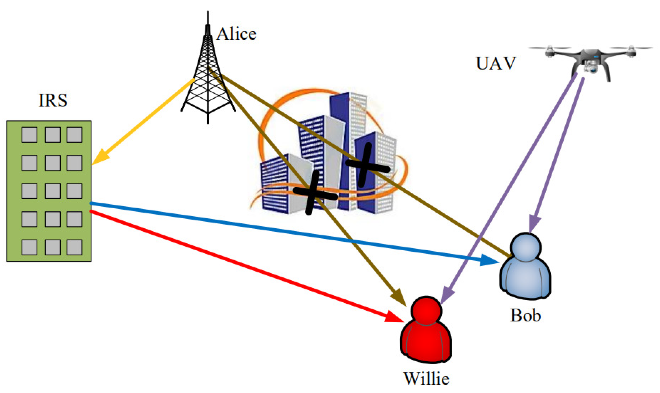
Figure 2.
The comparison of the optimal trajectory with the initial trajectory of the UAV.
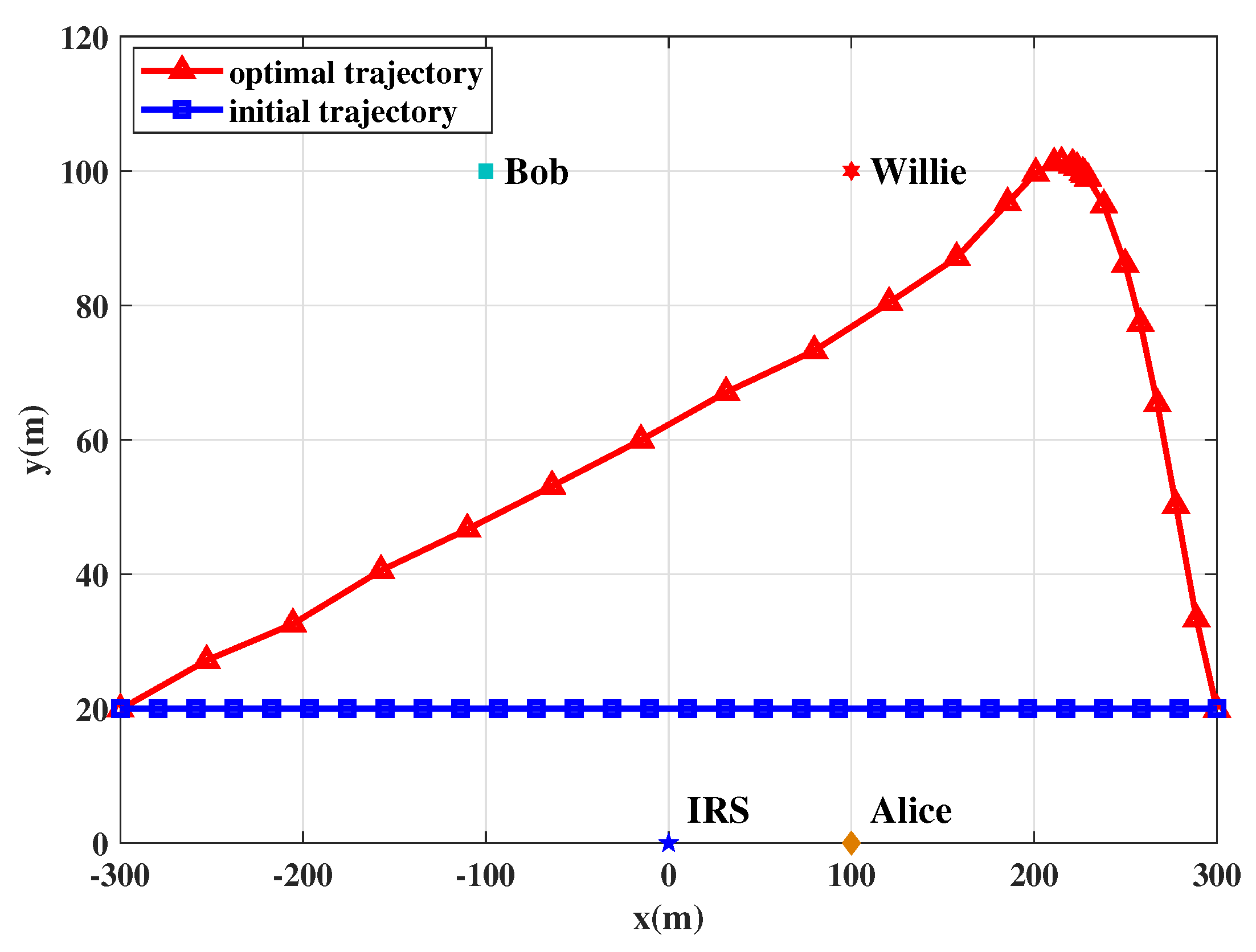
Figure 3.
The covert rate achieved by the system as the flying time varies, where M and H denote the number of IRS units and the height of UAV respectively.
Figure 3.
The covert rate achieved by the system as the flying time varies, where M and H denote the number of IRS units and the height of UAV respectively.
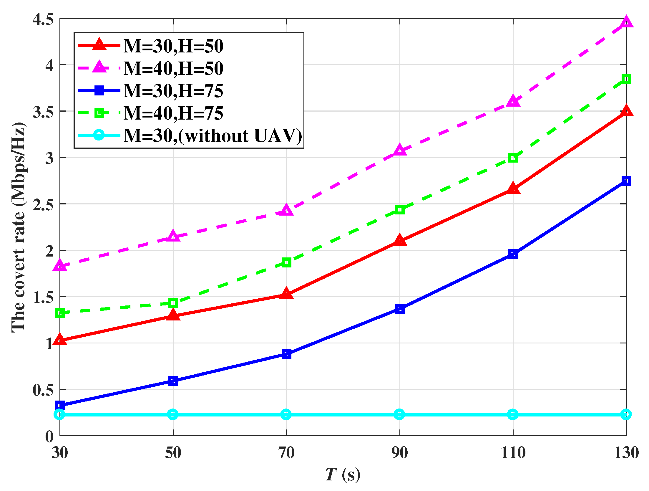
Figure 4.
The covert rate achieved by the system as the iteration time varies, where and denote the outage probability and the maximum speed of the UAV.
Figure 4.
The covert rate achieved by the system as the iteration time varies, where and denote the outage probability and the maximum speed of the UAV.
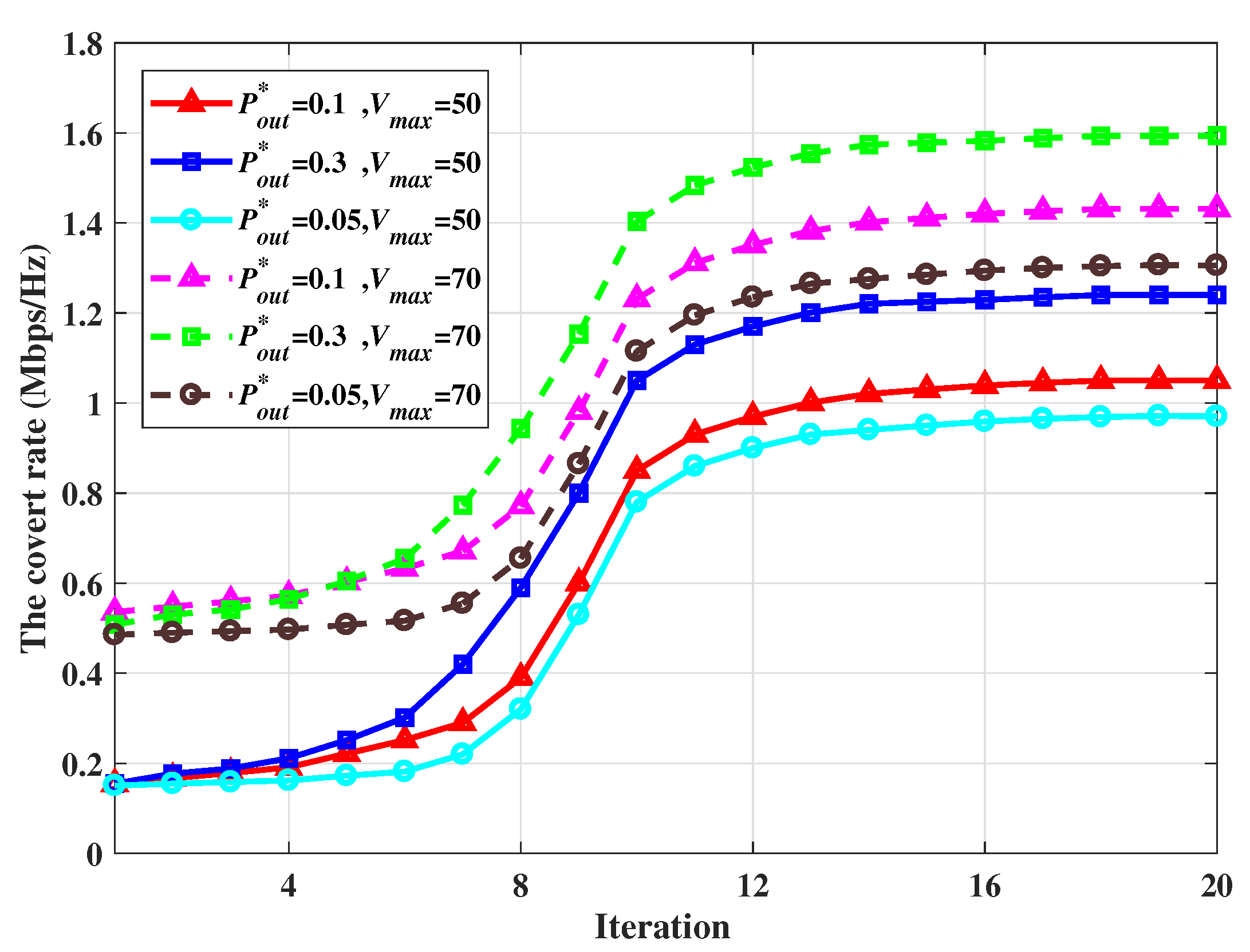
Figure 5.
The covert rate achieved by the system as the varies, where and denote the noise variances at Willie and Bob respectively.
Figure 5.
The covert rate achieved by the system as the varies, where and denote the noise variances at Willie and Bob respectively.
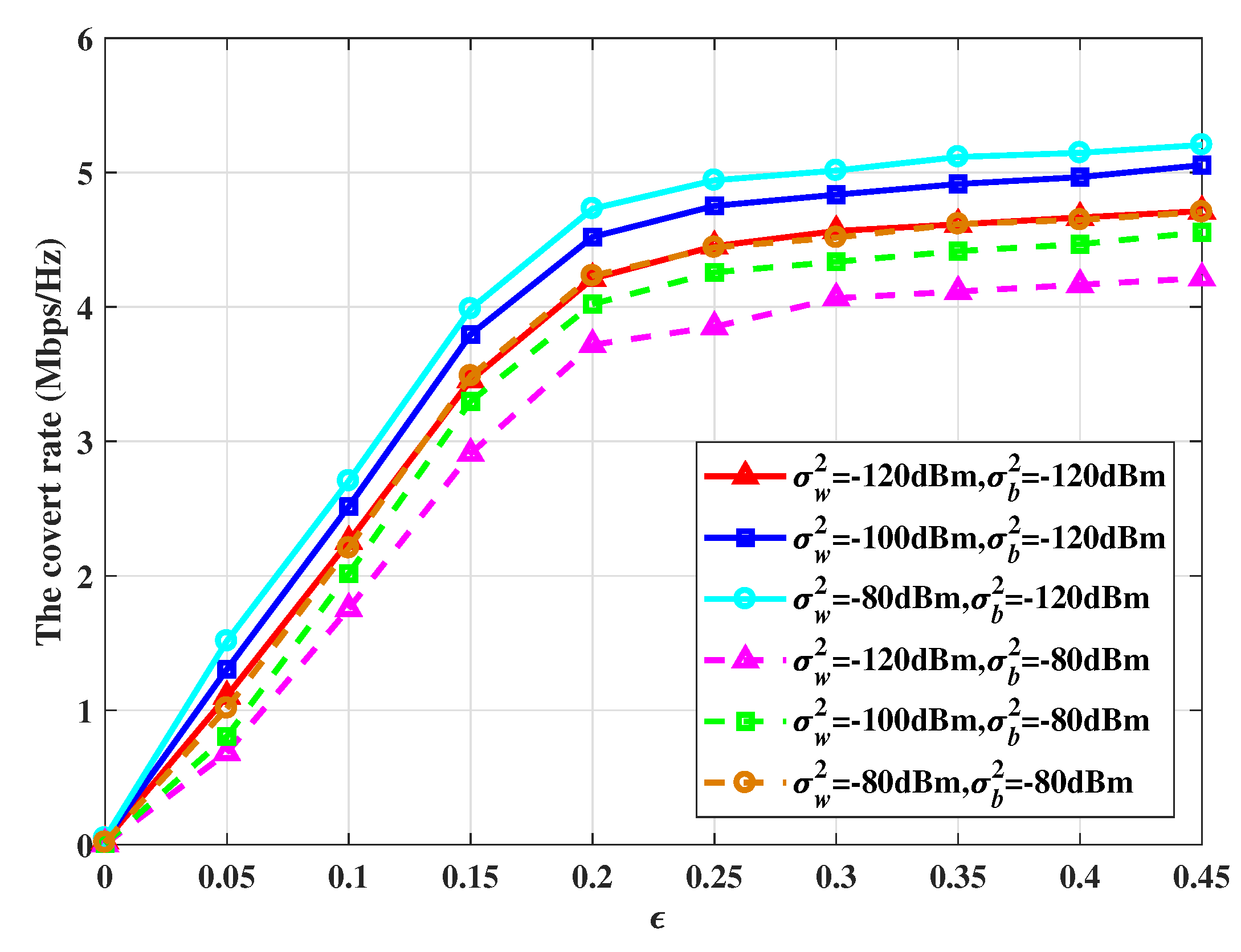
Figure 6.
The covert rate achieved by the system as the transmission power increases, where and T denote the maximum AN power and the flying time of UAV.
Figure 6.
The covert rate achieved by the system as the transmission power increases, where and T denote the maximum AN power and the flying time of UAV.
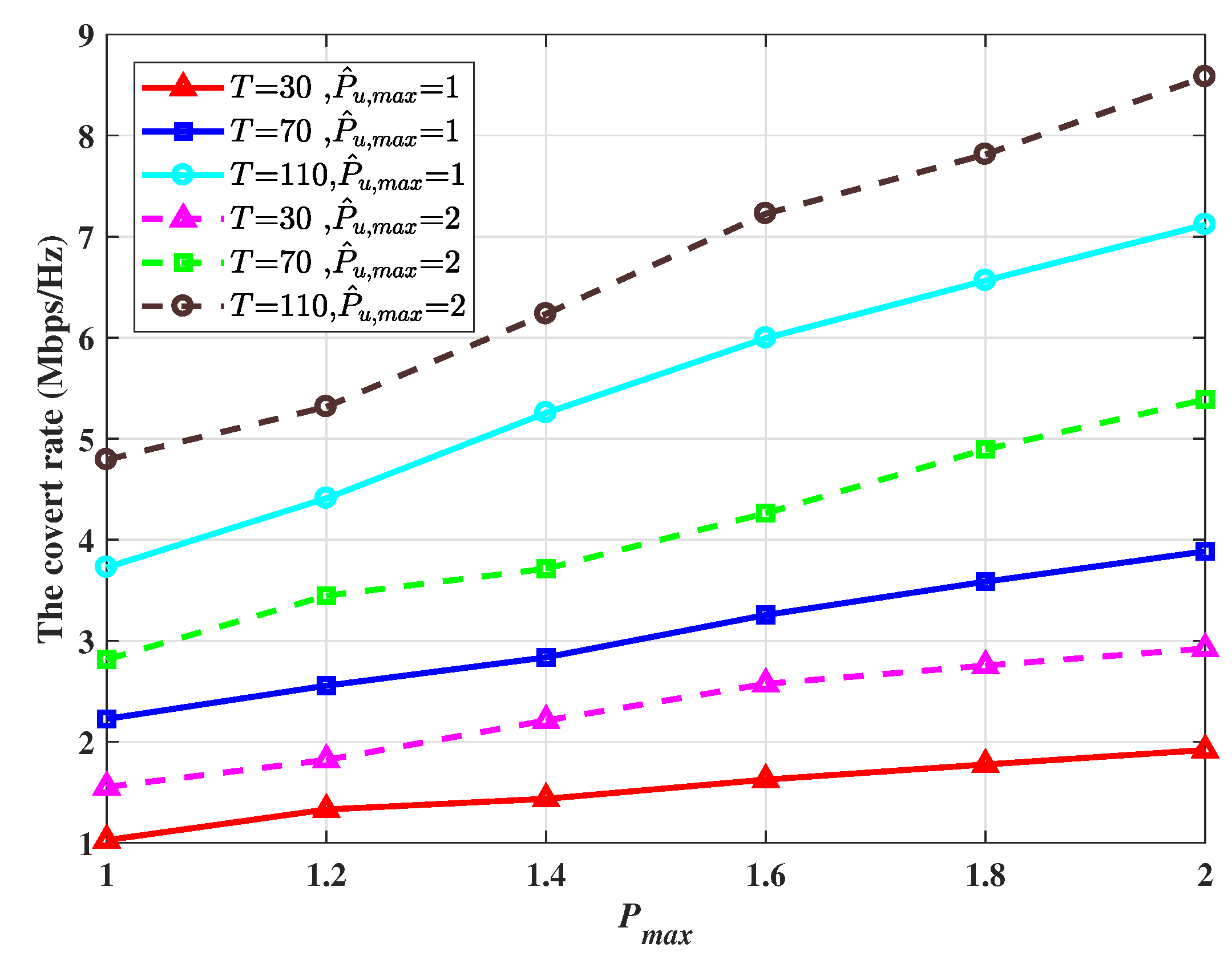

Table 1.
Simulation parameters
| Parameter | Meaning | Value |
|---|---|---|
| N | UAV flying time | 30s |
| T | Number of time slots | 30 |
| L | Duration of time slot | 1s |
| H | altitude of UAV | 50m |
| M | Number of IRS units | 30 |
| Maximum speed of UAV | 50m/s | |
| D | Maximum moving distance of UAV per time slot | 50m |
| Channel gain at a channel distance of 1m | -50dB | |
| Path loss parameter | 2.2 | |
| d | Antenna spacing | |
| P | Transmission power of BS | 1W |
| Parameters for quantifying noise uncertainty at Willie | 6dB | |
| Standard noise power variance at Willie | -120dBm | |
| Noise power variance at Bob | -120dBm | |
| Values for the covertness required at Willie | 0.01 | |
| J | Loop threshold | |
| Coordinates of Bob | ||
| Coordinates of Willie | ||
| Coordinates of base station | ||
| Initial coordinates of UAV | ||
| End coordinates of UAV |
Disclaimer/Publisher’s Note: The statements, opinions and data contained in all publications are solely those of the individual author(s) and contributor(s) and not of MDPI and/or the editor(s). MDPI and/or the editor(s) disclaim responsibility for any injury to people or property resulting from any ideas, methods, instructions or products referred to in the content. |
© 2023 by the authors. Licensee MDPI, Basel, Switzerland. This article is an open access article distributed under the terms and conditions of the Creative Commons Attribution (CC BY) license (http://creativecommons.org/licenses/by/4.0/).
Copyright: This open access article is published under a Creative Commons CC BY 4.0 license, which permit the free download, distribution, and reuse, provided that the author and preprint are cited in any reuse.


