
Submitted:
30 May 2023
Posted:
30 May 2023
You are already at the latest version
Abstract
We consider a specific holographic model in the limit where the gauge field does not couple to the rest of of the holographic fields (gravity and scalar sector) and investigate a phase of matter at zero charge density, a realistic feature that may have implications for disordered strange metals. We then pick a specific form of the gauge coupling $Z(\alpha)$ with a certain disorder realization and argue that this provides a hard-gapped insulator with exponentially-suppressed conductivity by holographic methods. The limit is non-trivial: as there is backreaction at zero density amount, surviving in the coupled case.
Keywords:
Holography
1. Introduction
We examined electrical transport in strongly coupled holographic quantum field theories at zero charge density, constructing perfect metals amidst disorder. Our findings have implications for realistic models of disordered strange metals.
2. Conductivity
Consider a static, asymptotically anti-de Sitter space with a black hole horizon sourced entirely by uncharged bulk matter and a dynamical metric. We can choose the bulk metric using diffeomorphism invariance.
indices represent the spatial boundary directions, while represent all dimensions, and L is AdS radius. All functions in the metric are functions of r and . We further choose bulk coordinate , with black hole horizon, and AdS boundary. Uncharged matter not required, energy conditions obeyed.
We add a U(1) gauge field to the bulk, so the action of our theory is
Function Z is a parameter of (uncharged) scalar matter, but for our purposes it’s an arbitrary function of r and . Gauge field’s two-point functions correspond to current-current correlation functions in the boundary theory, including electrical conductivity matrix . The conductivity may be related, via membrane paradigm [1], to data on the horizon of the black hole alone. The expected value of the boundary current is given by
where is the applied electric field, denotes a uniform spatial average, is the induced metric on the horizon, and is the unique function which obeys equation
with appropriate boundary conditions (for example, periodicity in compact boundary spatial directions). The membrane paradigm was used in holographic systems in [2], and similar computations appear in [3,4,5] for black holes with translational symmetry broken only in one direction. These results are special cases of this general formula. This formula may break down if black hole horizon fragments and becomes disconnected, as was considered in [6,7].
We can interpret (4) as a hydrostatic equation enforcing local charge conservation in an emergent horizon fluid. This is subtle – the local “electric current" in (4) is not the same as the expected value of the local current in the dual theory; only their spatial averages are equal. A powerful set of techniques have been developed to understand the qualitative behavior of transport in such fluids [8]; for example, it immediately follows from (4) that .
In particular, if is the conductivity matrix with given Z and :
If we set , (5) gives
If we expect that on average for a disordered sample, the conductivity matrix is isotropic (), that fixes conductivity to be , exactly the clean result!
A simple way to understand this result: suppose that in local coordinates, the metric is given by
Then we expect “locally" and [9]. On average and should have identical distributions, so we expect that and have the same distributions. This implies ; analogous statements are known for random resistor lattices in with analogous (e.g., log-normal) resistance distributions. And more generally, if is symmetrically distributed about 0, then in an isotropic theory, follows from (5) in the thermodynamic limit.
The robustness of in these strongly disordered models is remarkable, and deserves further comments. In models where momentum dissipation is introduced through massive gravity [10] or “Q-lattice" axions [11], one finds the hydrodynamic result [12]
where is charge density, energy density, P pressure, dissipative “quantum critical" conductivity without disorder, and a “momentum relaxation time", inversely related to graviton mass. Before now, it was unclear whether the fact that (8) holds beyond the hydrodynamic limit was an unrealistic feature of massive gravity or similar theories. Our work confirms this is a sensible prediction of massive gravity for many systems at . (8) further implies another mechanism, , by which the conductivity can reach its lower bound, . The conductivity saturating this lower bound, at least qualitatively, is likely to occur at strong disorder [8]. Confirmation that strongly-disordered charged holographic models (with ) have a conductivity no smaller than in would be a further non-trivial test of predictions of simple mean-field physics.
In , and/or if Z is distributed more generically, it’s valuable to employ insight gained from equivalence between Markov chains on lattices and resistance of a resistor lattice [13]. For arbitrary Z, this analogy can be leveraged to find lower and upper bounds to , for a self-averaging disordered sample: [8]
It is straightforward to test these results and bounds by numerically solving (4) for various disorder realizations. Good agreement with our exact analytic results and consistency with our bounds is obtained.
3. Conductor-Insulator Transition
(9) constrains to deviate from the clean result by the strength of fluctuations in Z and . It’s evident from (9) that if and Z are finite at all points on the horizon, then the black hole necessarily conducts electrical current, no matter how strong the disorder. This is a remarkable result. In contrast, in non-interacting quantum field theory, a conductor-insulator transition occurs at a finite disorder strength [14] in , and at arbitrarily small disorder in [15]. This transition relates to the destructive interference of matter waves scattering off of the disorder. Apparently, bulk fluctuations of the gauge field in holographic theories do not suffer from such interference. While it’s known [16,17] that metal-insulator transitions occur at a finite disorder strength in an interacting quantum system, even such systems ultimately succumb to (many-body) localization at strong disorder. Perhaps holographic models have taken the “coupling " limit first, rendering such a transition impossible.
Realizing a holographic conductor-insulator transition takes more care. A “helical lattice" approach has generated such a transition in [18,19], but there is no satisfying physical interpretation. However, even in these papers, the conductivity in the insulating phase only decays as algebraically in T as , in contrast to canonical insulators.
Assuming and a probe limit with AdS-Schwarzschild geometry, we need a large for , requiring percolating bubbles across the horizon. When these finite-Z regions disconnect, charge transport is halted, causing a disorder-driven holographic metal-insulator transition, similar to random resistor lattices [20].
Numerically compute conductivity for Z ansatz with "bubbles" where percolate across horizon to test proposal. Numerics support this; see Figure 1 and Figure 2.
3.1. Holographic Realizations
We now ask whether the percolation mechanism proposed above for a disorder-driven metal-insulator transition can occur in a “realistic" holographic model: a bottom-up Einstein-Maxwell-dilaton ()-axion () theory with action
Here is a mass scale, whose precise value is unimportant – we choose it so that is strictly dimensionless, for simplicity, and
At , generalizing choices yields similar results, but (10) with axio-dilaton scalar kinetic terms is essential. ’s cosine potentials may suit our needs, and arise due to instanton effects in effective actions (as in QCD). In our holographic model, isn’t suppressed by (the scale of bulk’s quantum corrections).
For conductor-insulator transitions, must have at least two minima, and , with and . drives the transition and stabilizes it, although theories with finite Lifshitz or hyperscaling-violating exponents may also work [21]. Insulators form when bubbles of percolate across the horizon; we aim to demonstrate how to create and maintain these bubbles at low temperatures. [21] is a citation. For this purpose, a simple choice of potentials, though certainly not the only, is
Using Z in [22], we set , , and marginal to avoid axion backreaction on the dilaton. The Harris criterion [21] implies inability to source disordered modes of all wavelengths without UV geometry backreaction.
Let us begin by sourcing the dilaton with (positive) -like sources on the AdS boundary – analogous to point-like impurities in the dual theory. Each impurity produces an expanding bubble which becomes insulating; width of the “bubbles" of is . If density of the impurities is n, then the bubbles percolate across the horizon when . Within each bubble, , and thus at low temperatures we obtain an insulator
A second mechanism for obtaining the transition is as follows: suppose .
As in the insulating phase, we predict:
4. Outlook
Recent models [23,24,25,26] propose momentum non-conservation in (quasi-2d) strange metals. We constructed perfect conductors in strong disorder and predict finite charge density will not decrease conductivity. We encourage extending holographic approach to charged black holes and finding non-holographic field theories with disorder-resistant .
Acknowledgments
We thank Ed Witten for discussions. We especially thank Veronica Toro Arana and Anna Maria Wojtyra for providing some code for solving elliptic partial differential equations. This research was funded through Nvidia.
References
- K. S. Thorne, R. H. Price, and D. A. MacDonald (eds.). Black Holes: The Membrane Paradigm (Yale University Press, 1986).
- N. Iqbal and H. Liu. “Universality of the hydrodynamic limit in AdS/CFT and the membrane paradigm", Physical Review D79 025023 (2009). arXiv:0809.3808.
- S. Ryu, T. Takayanagi, and T. Ugajin. “Holographic conductivity in disordered systems", Journal of High Energy Physics 04 115 (2011). arXiv:1103.6068.
- A. Donos and J. P. Gauntlett. “The thermoelectric properties of inhomogeneous holographic lattices", Journal of High Energy Physics 01 035 (2015). arXiv:1409.6875.
- M. Rangamani, M. Rozali, and D. Smyth. “Spatial modulation and conductivities in effective holographic theories". arXiv:1505.05171.
- D. Anninos, T. Anous, F. Denef, and L. Peeters. “Holographic vitrification". arXiv:1309.0146.
- G. T. Horowitz, N. Iqbal, J. E. Santos, and B. Way. “Hovering black holes from charged defects", Classical & Quantum Gravity 32 105001 (2015). arXiv:1412.1830.
- A. Lucas. “Hydrostatic transport in strongly coupled disordered quantum field theories", to appear.
- P. Chesler, A. Lucas, and S. Sachdev. “Conformal field theories in a periodic potential: results from holography and field theory", Physical Review D89 026005 (2014). arXiv:1308.0329.
- M. Blake and D. Tong. “Universal resistivity from holographic massive gravity", Physical Review D88 106004 (2013). arXiv:1308.4970.
- B. Goutéraux. “Charge transport in holography with momentum dissipation", Journal of High Energy Physics 04 181 (2014). arXiv:1401.5436.
- S. A. Hartnoll, P. K. Kovtun, M. Müller, and S. Sachdev. “Theory of the Nernst effect near quantum phase transitions in condensed matter, and in dyonic black holes", Physical Review B76 144502 (2007). arXiv:0706.3215.
- D. A. Levin, Y. Peres, and E. L. Wilmer. Markov Chains and Mixing Times (AMS, 2009).
- P. W. Anderson. “Absence of diffusion in certain random lattices", Physical Review 109 1492 (1958).
- E. Abrahams, P. W. Anderson, D. C. Licciardello, and T. V. Ramakrishnan. “Scaling theory of localization: absence of quantum diffusion in two dimensions", Physical Review Letters 42 673 (1979).
- T. Giamarchi and H. J. Schulz. “Localization and interaction in one-dimensional quantum fluids", Europhysics Letters 3 1287 (1987).
- D. M. Basko, I. L. Aleiner, and B. L. Altshuler. “Metal-insulator transition in a weakly interacting many-electron system with localized single-particle states", Annals of Physics 321 1126 (2006). arXiv:cond-mat/0506617.
- A. Donos and S. A. Hartnoll. “Interaction-driven localization in holography", Nature Physics 9 649 (2013). arXiv:1212.2998.
- A. Donos, B. Goutéraux, and E. Kiritsis. “Holographic metals and insulators with helical symmetry", Journal of High Energy Physics 09 038 (2014). arXiv:1406.6351.
- B. Derrida and J. Vannimenus. “A transfer-matrix approach to random resistor networks", Journal of Physics A15 L557 (1982).
- A. Lucas, S. Sachdev, and K. Schalm. “Scale-invariant hyperscaling-violating holographic theories and the resistivity of strange metals with random-field disorder", Physical Review D89 066018 (2014). arXiv:1401.7993.
- E. Mefford and G. T. Horowitz. “Simple holographic insulator", Physical Review D90 084042 (2014). arXiv:1406.4188.
- S. A. Hartnoll. “Theory of universal incoherent metallic transport", Nature Physics 11 54 (2015). arXiv:1405.3651.
- P. Kovtun. “Fluctuation bounds on charge and heat diffusion". arXiv:1407.0690.
- S. A. Hartnoll and A. Karch. “Scaling theory of the cuprate strange metals", Physical Review B91 155126 (2015). arXiv:1501.03165.
- D. V. Khveshchenko. “Constructing (un)successful phenomenologies of the normal state of cuprates". arXiv:1502.03375.
Figure 1.
from a black hole horizon for a theory in ; we set , and use periodic boundary conditions with , with a discretized spatial grid of points. We take and , where , with and independent random phases, and is a random constant. We took various values of B and fixed . When , curves at different B approximately collapse, implying that current avoids the non-conducting bubbles; when , the value of conductivity is sensitive to B. In the limit and , a metal-insulator transition appears at .
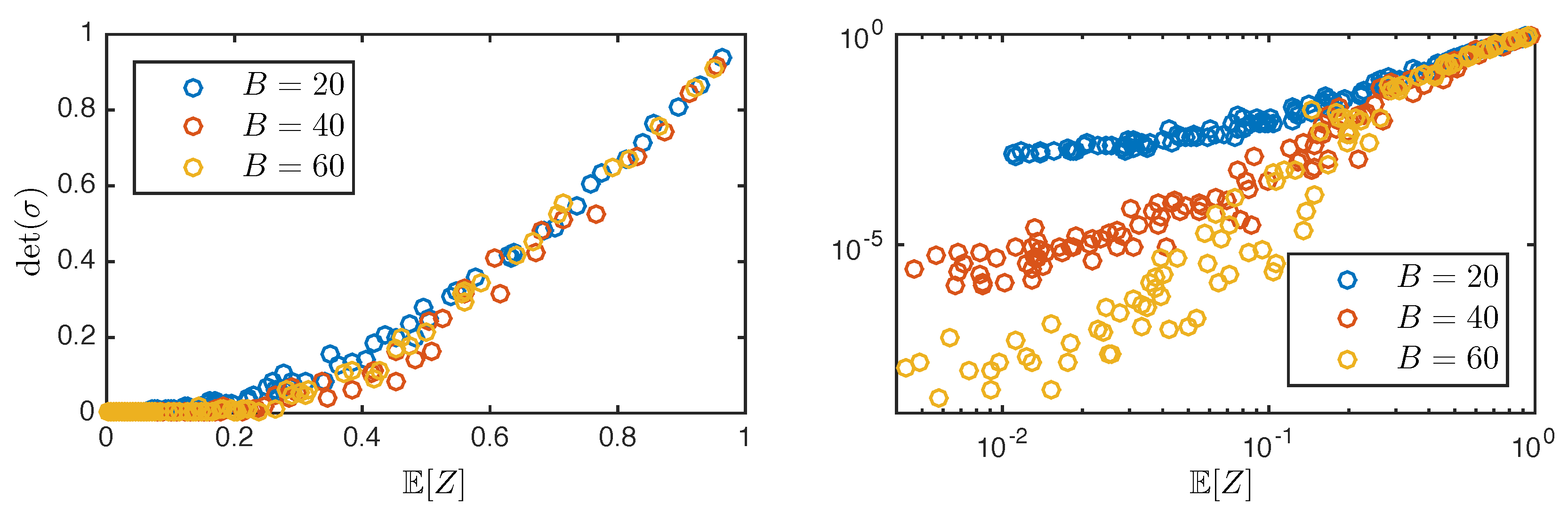
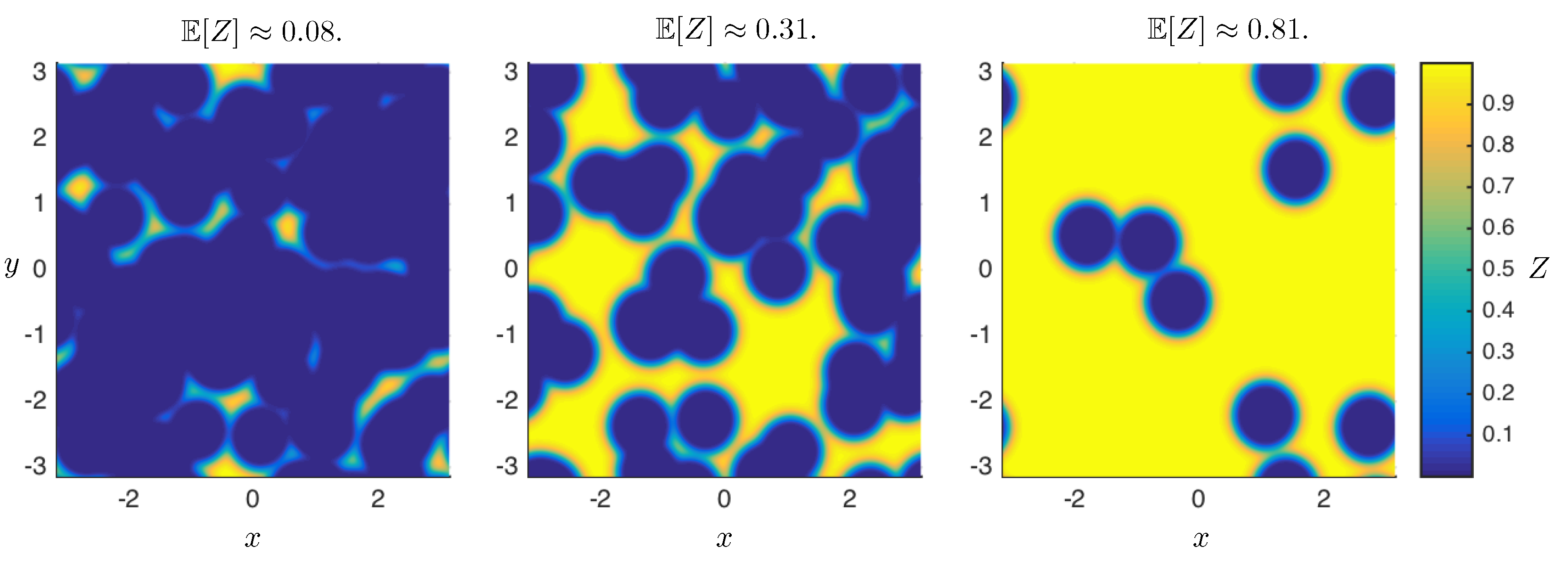
Figure 2.
Surface plots of for various bubble densities. Depending on whether regions of high or low Z percolate across the horizon determines whether we’re in the metallic or insulating phase, as is clear upon comparing with Figure 1.
Figure 2.
Surface plots of for various bubble densities. Depending on whether regions of high or low Z percolate across the horizon determines whether we’re in the metallic or insulating phase, as is clear upon comparing with Figure 1.
Disclaimer/Publisher’s Note: The statements, opinions and data contained in all publications are solely those of the individual author(s) and contributor(s) and not of MDPI and/or the editor(s). MDPI and/or the editor(s) disclaim responsibility for any injury to people or property resulting from any ideas, methods, instructions or products referred to in the content. |
© 2020 by the author. Licensee MDPI, Basel, Switzerland. This article is an open access article distributed under the terms and conditions of the Creative Commons Attribution (CC BY) license (https://creativecommons.org/licenses/by/4.0/).
Copyright: This open access article is published under a Creative Commons CC BY 4.0 license, which permit the free download, distribution, and reuse, provided that the author and preprint are cited in any reuse.


