Submitted:
29 May 2023
Posted:
30 May 2023
Read the latest preprint version here
Abstract
The aim of this paper is the analysis of isotropic rectangular Kirchhoff plates with two opposite edges clamped and the other edges having various support conditions. Rectangular Kirchhoff plates with two opposite edges simply supported are usually analyzed using the simple trigonometric series of Lévy or the double trigonometric series of Navier, while the loads are expanded in Fourier series. In this paper the flexibility method (or force method) of the linear beam theory was applied whereby the unknowns were the bending moments along the opposite edges; in this regard, the primary system was the plate simply supported along the above-mentioned opposite edges and subjected to the external loads, system solved using the Lévy solution, and the redundant system was the plate simply supported along the opposite edges and subjected to bending moments along those edges. In the redundant system, a modified Lévy solution was introduced to account for the edge moments. The compatibility equations (vanishing of the slopes at selected positions of the opposite edges) were set to determine the unknowns and so the efforts in the plate. The results obtained were in good agreement with the exact results.
Keywords:
Isotropic rectangular Kirchhoff plate
; opposite edges clamped
; flexibility method
; force method
; Lévy solution
; Fourier sine series
1. Introduction
The Kirchhoff–Love plate theory (KLPT) was developed in 1888 by Love using assumptions proposed by Kirchhoff [1]. The KLPT is governed by the Germain−Lagrange plate equation; this equation was first derived by Lagrange in December 1811 in correcting the work of Germain [2] who provided the basis of the theory. For rectangular plates, Navier [3] in 1820 introduced a simple method for the analysis when a plate is simply supported along all edges; the applied load and the deflection were expressed in terms of Fourier components and double trigonometric series, respectively. Another approach was proposed by Lévy [4] in 1899 for rectangular plates simply supported along two opposite edges; the applied load and the deflection were expressed in terms of Fourier components and simple trigonometric series, respectively. Many exact solutions for isotropic linear elastic thin plates have been developed by Timoshenko [5]; the simple trigonometric series of Lévy was mostly considered. Mama et al. [6] presented the single finite Fourier sine integral transform method for the flexural analysis of rectangular Kirchhoff plate with opposite edges simply supported, and the other edges clamped for the case of triangular load distribution on the plate domain. Sayyad et al. [7] assessed a trigonometric plate theory for the static bending analysis of plates resting on Winkler elastic foundation; the theory considered the effects of transverse shear and normal strains. Xu et al. [8] got exact solutions for rectangular anisotropic plates with four clamped edges through the state space method whereby the Fourier series in exponential form were adopted. Khan et al. [9] used the variational approach to investigate a clamped rectangular plate under a uniform load; the minimum total potential energy approach was considered. Onyia et al. [10] presented the elastic buckling analysis of rectangular thin plates using the single finite Fourier sine integral transform method. Pisacic et al. [11] developed a procedure of calculating deflection of rectangular plate using a finite difference method, programmed in Wolfram Mathematica; the system of equations was built using the mapping function and solved with solve function. Delyavskyy et al. [12] developed an approach to analyze thin isotr opic symmetrical plates using combined analytical and numerical methods. Imrak et al. [14] presented an exact solution for a rectangular plate clamped along all edges in which each term of the series is trigonometric and hyperbolic, and identically satisfies the boundary conditions on all four edges.
In this paper, isotropic rectangular Kirchhoff plates with two opposite edges clamped and the other edges having various support conditions are analyzed. The plate is modeled as the superposition of two systems: 1) the plate simply supported at the opposite edges and subjected to the external loads, this system being solved using the Lévy solution, 2) the plate simply supported at the opposite edges and subjected to edge moments loading. Given that the Lévy solution is not able to model plate edges subjected to a moment loading, a modified Lévy solution will be introduced to account for the edge moments. Therefore, the flexibility method can be applied to determine the efforts and deformations of the plate.
2. Materials and methods
2.1. Governing equations of the plate
The Kirchhoff–Love plate theory (KLPT) [1] is used for thin plates whereby shear deformations are not considered. The spatial axis convention (X, Y, Z) is represented in Figure 1 below.
The equations of the present section are related to the KLPT. The governing equation of the isotropic Kirchhoff plate, derived by Lagrange, is given by
where w(x,y,z) is the displacement in z-direction, q(x,y) the applied transverse load per unit area, and D the flexural rigidity of the plate.
The bending moments per unit length mxx and myy, and the twisting moments per unit length mxy are given by
The Kirchhoff shear forces per unit length combine shear forces and twisting moments, and can be expressed as follows:
In these equations, E is the elastic modulus of the plate material, h is the plate thickness, and ν is the Poisson’s ratio.
2.2. Rectangular isotropic plate clamped along two opposite edges
The analyzed rectangular plate is assumed clamped along two opposite edges. The flexibility method (or force method) of the linear beam theory was applied in this analysis whereby the unknowns were the bending moments along the opposite edges. In this regard the primary system was the plate simply supported along the above mentioned opposite edges and the redundant system was the plate subjected to bending moments along those edges. The compatibility equations (vanishing of the slopes along the opposite edges) were used to determine the unknowns.
2.2.1. Primary problem: plate simply supported along two opposite edges
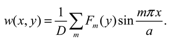
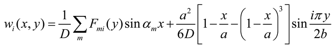
The plate dimensions in x- and y-direction are denoted by a and b, respectively. The rectangular plate is assumed simply supported along the edges x = 0 and x = a. The solution by Lévy [4] that satisfies the boundary conditions at these edges is considered for the deflection curve w(x,y) as follows:
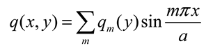
The Fourier sine series of the transverse applied load is given by
Substituting Equations (4) and (5) into (1) yields the differential equation
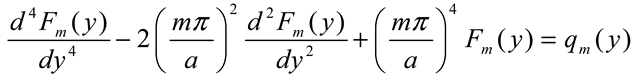
The solution to Equation (6) is as follows:
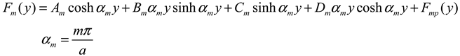 where the coefficients Am, Bm, Cm, and Dm are determined by satisfying the boundary and continuity conditions in y-direction, and Fmp(y) is a particular solution to the differential equation.
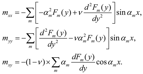
Substituting Equation (4) into (2a-c) yields the equations of bending moments and twisting moments as follows:
With regard to the boundary conditions at y = 0 and y = b the equations for the slope ∂w/∂y and the bending moment myy are set using Equations (4), (7), and (8b) as follows
Furthermore, with regard to the boundary conditions at y = 0 and y = b the Kirchhoff shear force Vy is calculated by substituting Equations (4) and (7) into (3b) as follows:
In summary, the boundary conditions at y = 0 and y = b needed to determine the coefficients Am, Bm, Cm, and Dm.are expressed using the equations for the deflection (Equations (4) and (7)), the slope ∂w/∂y (Equation (9a)), the bending moment myy (Equation (9b)), and the Kirchhoff shear force Vyy (Equation (9c)).
The flexibilities δj0 (slopes at positions j of the opposite edges where the compatibility equations will be set) for the primary problem are calculated using Equations (4) and (7) as follows:
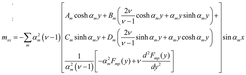
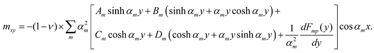
For the primary problem the bending moments myy are calculated using Equations (9b), and the bending moments mxx and twisting moments mxy are calculated using Equations (7) and (8a,c) as follows
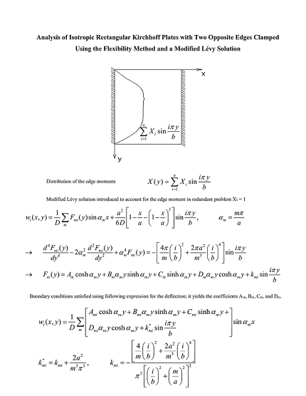
2.2.2. Redundant problem: plate subjected to a distributed moment along the edge x = 0
The distribution of the bending moments X(y) along the clamped edge x = 0 depends on the support conditions along the edges y = 0 and y = b, namely supported (simply supported or clamped) or free.
Edges y = 0 and y = b simply supported or clamped Redundant problem Xi = 1
The edges y = 0 and y = b are assumed simply supported or clamped. Observing that the bending moments vanish at angles supported in two directions (in this case at y= 0 and y = b), the distribution of the bending moments X(y) along the clamped edge x = 0 can be described with the following trigonometric series
Here, the redundant effort is a distributed bending moment sin (iπy/b) along the edge x = 0 according to Equation (12).
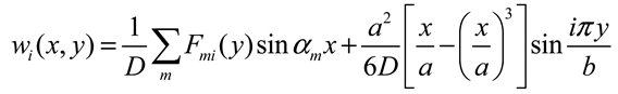
To account for the edge moments the solution by Lévy [4] for the transverse displacement can be modified as follows
The second term on the right-hand side of Equation (13) is the displacement function of a plate strip simply supported at its ends and subjected at the edge x = 0 to a distributed moment sin (iπy/b). It is noted that Equation (13) satisfies the boundary conditions at edges x = 0 and x = a. Substituting Equation (13) into (1) yields
The following functions contained in Equation (14) are expanded in Fourier sine series
Substituting Equations (15) into (14) yields
Given that Equation (16) holds for any value of x, it results the following differential equation
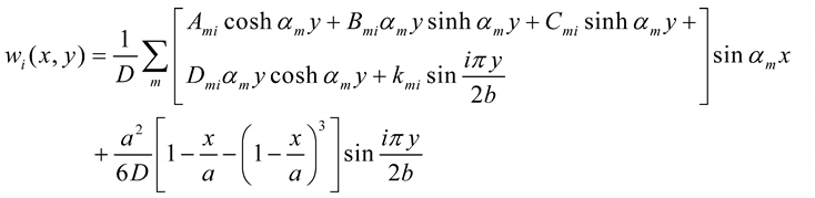
The solution to Equation (17) is identical to Equation (7) whereby the particular solution is given by
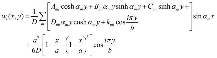
Combining Equations (7), (13) and (18) yields the transverse displacement function as follows
To satisfy the boundary conditions at y = 0 and y = b, the Fourier series of Equation (15) is used; Equation (19) becomes
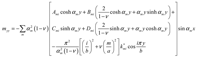
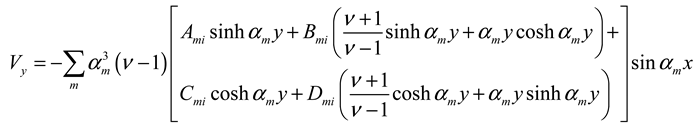
With respect to the boundary conditions at y = 0 and y = b the equations for the slope ∂w/∂y and the bending moment myy are set using Equations (9a-b) and (20) as follows
In summary, the boundary conditions at y = 0 and y = b needed to determine the coefficients Ami, Bmi, Cmi, and Dmi.are expressed using Equations (20) and (21a-b)
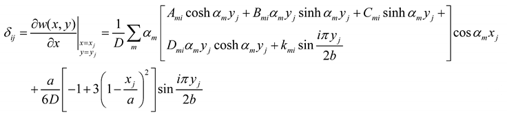
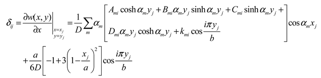
The flexibilities δij (slopes at relevant positions j (xj, yj) of the opposite edges where the compatibility equations will be set) for the redundant problem Xi = 1 are calculated using Equation (19); it yields
The positions j must be chosen such that they are regularly distributed along the clamped edge. Recalling that there should be as many redundants as compatibility equations, for an edge with n redundants considered the positions yi = k×b/ (n + 1) with k = 1, 2, 3 …n as represented in Figure 2a can be taken.
In case of system and loading symmetrical with respect to axis y = b/2 only odd values of i need be considered, the redundants being zero for even values; and in case of system symmetrical and loading anti symmetrical with respect to axis y = b/2 only even values of i need be considered, the redundants being zero for odd values. In both cases, the flexibilities and compatibility equations can be set in half of the structure in y–direction. Given the half edge having n redundants, the positions yi = k×b/2n with k = 1, 2, 3 …n as represented in Figure 2b can be taken.
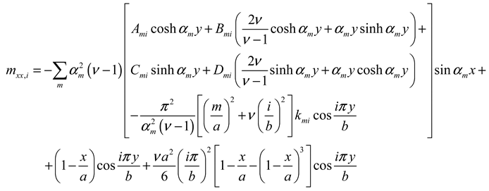
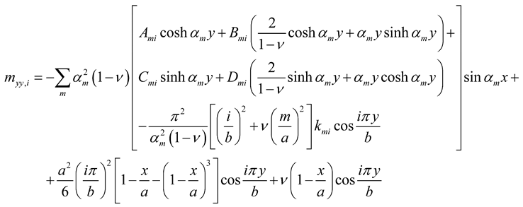
For the redundant problem Xi = 1 the bending moments mxx and myy , and the twisting moments mxy are calculated using Equations (2a-c) and (19):
According to the flexibility method of the theory of elasticity, the compatibility equations are established so as to restore the geometric boundary conditions of the clamped edges (vanishing of slopes ∂w/∂x at selected positions of the edge). Assuming a plate with n redundant, the compatibility equations for the position yi can be expressed as follows
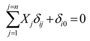 δi0 and δij being the flexibility coefficients in the primary problem and in the redundant problems, respectively. Equation (24) is established at any selected position and so the redundant efforts are determined. The efforts in the plate are then calculated as follows
S0 and Sj being the efforts in the primary problem and in the redundant problem, respectively.
Edge y = 0 simply supported or clamped, and edge y = b free Redundant problem Xi = 1
The edge y = 0 is simply supported or clamped and y = b is free. The analysis in this section is valid if the edge y = 0 is free and y = b is simply supported or clamped; the results must be appropriately inverted.
Observing that the bending moments X(y) vanish at y = 0 (angle supported in two directions), their distribution along the clamped edge x = 0 can be described with the following trigonometric series
i being an odd number . The redundant effort is a distributed bending moment sin (iπy/2b) along the edge x = 0 according to Equation (26).
To account for the edge moments the solution by Lévy [4] for the transverse displacement can be modified as follows
The analysis continues similarly to Section 2.2.2.1. The differential equation (Equation (17)) becomes
The solution to Equation (28) is identical to Equation (7) whereby the particular solution is given by
Therefore the transverse displacement function is as follows
To satisfy the boundary conditions at y = 0 and y = b, the Fourier series of Equation (15) is used; Equation (30) becomes
With respect to the boundary conditions at y = 0 and y = b the equations for the slope ∂w/∂y and the bending moment myy are set using Equations (8b) and (31) as follows
Furthermore, with regard to the boundary conditions at y = b the Kirchhoff shear force is calculated using Equations (31) and (9c). It is noted that the first and third derivatives of the term with sin (iπy/2b) contain cos (iπy/2b) ¨that vanishes at y = b. It results
In summary the boundary conditions at y = 0 and y = b are expressed using Equations (31), (32a-b), and (33); they permit to determine the coefficients Ami, Bmi, Cmi, and Dmi.
The flexibilities δij (slopes at relevant positions j (xj, yj) of the opposite edges where the compatibility equations will be set) for the redundant problem Xi = 1 are calculated using Equation (30) as follows
Given n redundants considered, the positions yi = k×b/n with k = 1, 2, 3 …n as represented in Figure 3 can be taken.
For the redundant problem the bending moments mxx and myy and the twisting moments mxy are calculated using Equations (2a-c) and (30):
The compatibility equations and the efforts in the plate are calculated using Equations (24) and (25).
Edges y = 0 and y = b free Redundant problem Xi = 1
The edges y = 0 and y = b are free. Observing that the bending moments X(y) have non zero values at the angles, their distribution along the clamped edge x = 0 can be described with the following trigonometric series
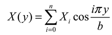
The redundant effort is a distributed bending moment cos (iπy/b) along the edge x = 0 according to Equation (36).
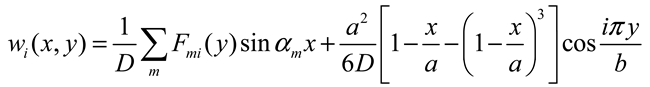
To account for the edge moments the solution by Lévy [4] for the transverse displacement can be modified as follows
The analysis continues similarly to Section 2.2.2.1. The differential equation (Equation (17)) becomes
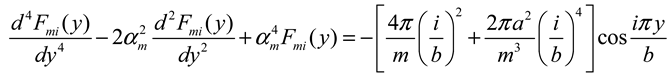
The solution to Equation (38) is identical to Equation (7) whereby the particular solution is given by
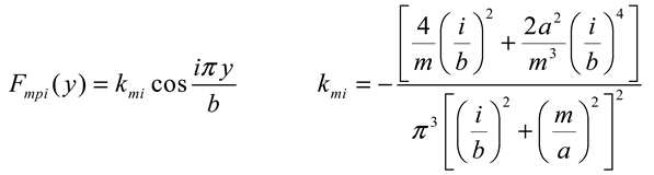
Therefore, the transverse displacement function is as follows
To satisfy the boundary conditions at y = 0 and y = b, the Fourier series of Equation (15) is used; Equation (40) becomes
With regard to the boundary conditions at y = 0 and y = b the equation for the bending moment myy is set using Equations (8b) and (41) as follows
Furthermore, with regard to the boundary conditions at y = 0 and y = b the Kirchhoff shear force is calculated using Equations (41) and (9c). It is noted that the first and third derivatives of the term with cos (iπy/b) contain sin (iπy/b) that vanishes at y = 0 and y = b. It results at y = 0 and y = b
In summary the boundary conditions at y = 0 and y = b are expressed using Equations (42) and (43); they permit to determine the coefficients Am, Bm, Cm, and Dm.
The flexibilities δij (slopes at relevant positions j (xj, yj) of the opposite edges where the compatibility equations will be set) for the redundant problem Xi = 1 are calculated using Equation (40) as follows
Given n redundants considered, the positions yi = k×b/(n – 1) with k = 0, 1, 2, 3 …n - 1 as represented in Figure 4a can be taken.
In case of loading symmetrical with respect to axis y = b/2 only even values of i need be considered, the redundants being zero for odd values; and in case of loading anti symmetrical with respect to axis y = b/2 only odd values of i need be considered, the redundants being zero for even values. In both cases, the flexibilities and compatibility equations can be set in half of the structure in y–direction. Given the half edge having n redundants, the positions yi = k×b/2(n – 1) with k = 0, 1, 2, 3 …n - 1 as represented in Figure 4b can be taken.
For the redundant problem Xi = 1 the bending moments mxx and myy and the twisting moments mxy are calculated using Equations (2a-c) and (40):
The compatibility equations and the efforts in the plate are calculated using Equations (24) and (25).
2.2.3. Redundant problem: plate subjected to a distributed end moment along the edge x = a
The edges x = 0 and x = a are assumed clamped. Given the symmetrical nature of the plate with respect to the axis x = a/2, the positions along the edge x = a where the compatibility equations are set will be taken identical to those of edge x = 0. Therefore, the bending moments mxx and myy and twisting moments mxy for redundant effort are the same as in Section 2.2.2; however the flexibilities, defined as slopes in this study, will be affected with a minus sign to the corresponding values for the case of bending moments acting along the edge x = 0.
Else, the analysis could be conducted similarly to Section 2.2.2, whereby the modified Lévy solution for edges y = 0 and y = b supported e.g. would be given by
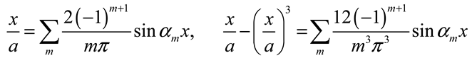
Following Fourier sine series expansions are useful in the analysis
3. Results and discussion
3.1. Plate clamped along the edges x = 0, y = 0 and y = b and simply supported along x = a
The analysis of a rectangular plate clamped along the edges x = 0, y = 0 and y = b and simply supported along the edge x = a and subjected to a uniformly distributed load q was conducted whereby the Poisson’s ratio was not considered. The plate dimensions in x- and y-directions are denoted by a and b, respectively. The calculated bending moments at the middle of the clamped edge x = 0 are mx,cl = -qa2/Nx,cl and those at the middle of the plate are mxm = qa2/Nxm and mym = qa2/Nym. Detailed results are presented in the Supplementary Material “Rectangular plate clamped and simply supported.” Table 1 lists the results, depending on the ratio b/a, obtained using the tables by Czerny [14] (exact results) and those obtained in the present study whereby one redundant (i = 1 for the position yj = b/2), three redundants (i = 1, 3, and 5 for the positions yj = b/10, 3b/10, and b/2), and five redundants (i = 1, 3, 5, 7, and 9 for the positions yj = b/10, b/5, 3b/10, 2b/5, and b/2) were considered. It is recalled that only half of the structure in y–direction and odd values of i are taken since the system and loading are symmetrical with respect to axis y = b/2.
As Table 1 shows, the results of the present study show good agreement with the exact results. The accuracy should be increased by considering more redundants (high values of i) since the geometric boundary conditions of the original structure (vanishing of the slopes along the opposite edges) should be restored all over the clamped edge and not only at selected positions.
3.2. Rectangular plate clamped along all edges
A rectangular plate clamped along all edges and subjected to a uniformly distributed load q was analyzed whereby the Poisson’s ratio was not considered. The plate dimensions in x- and y-directions are denoted by a and b, respectively. The calculated bending moments at the middle of the clamped edge x = 0, a and y = 0, b are mx,cl = -qa2/Nx,cl and my,cl = -qa2/Ny,cl , respectively, and those at the middle of the plate are mxm = qa2/Nxm and mym = qa2/Nym. Detailed results are presented in the Supplementary Material “Rectangular plate clamped along all edges.” Table 2 lists the results, depending on the ratio b/a, obtained using the tables by Czerny [14] (exact results) and those obtained in the present study whereby at edges x = 0 and x = a one redundant (i = 1 for the position yj = b/2) and three redundants (i = 1, 3, and 5 for the positions yj = b/10, 3b/10, and b/2) were considered. It is recalled that only half of the structure in y–direction and odd values of i are taken since the system and loading are symmetrical with respect to axis y = b/2.
As Table 2 shows, the results of the present study show good agreement with the exact results. The accuracy should be increased by considering more redundants (high values of i).
3.3. Rectangular plate clamped along x = 0, simply supported along x = a and y = 0, and free along y = b
The analysis of a plate clamped along the edge x = 0, simply supported along x = a and y = 0, and free along y = b and subjected to a uniformly distributed load q was conducted whereby the Poisson’s ratio was not considered. The plate dimensions in x- and y-directions are denoted by a and b, respectively. The calculated bending moment at the end of the clamped edge x = 0 is mx,fre = -qb2/Nx,fre, in the middle of the free edge mx,frm = qb2/Nx,frm, and in the middle of the plate mxm = qb2/Nxm and mym = qb2/Nym. Details of the results are presented in the Supplementary Material “Rectangular plate clamped simply supported and free.” Table 3 lists the results, depending on the ratio b/a, obtained using the tables by Czerny [14] (exact results) and those obtained in the present study whereby one redundant (i = 1 for the position yj = b), three redundants (i = 1, 3, and 5 for the positions yj = b/5, 3b/5, and b), and five redundants (i = 1, 3, 5, 7, and 9 for the positions yj = b/5, 2b/5, 3b/5, 4b/5, and b) were considered.
As Table 3 shows, the results of the present study show good agreement with the exact results. The accuracy is increased by considering more redundants.
4. Conclusions
Isotropic rectangular Kirchhoff plates clamped along two opposite edges were analyzed in this paper. The flexibility method (or force method) of the linear beam theory was applied whereby the unknowns were the bending moments along the opposite edges; in this regard the primary system was the plate simply supported along the above mentioned opposite edges and subjected to the external loads and the redundant system was the plate subjected to bending moments along those edges. We showed that the solution by Lévy [4] commonly used in the case of simply supported opposite edges can be extended, with some adjustment, to simply supported opposite edges subjected to edge moment loading. The compatibility equations (vanishing of the slopes at selected positions of the clamped edge) were set to determine the unknowns and so the efforts in the plate. Numerical results were presented and showed good agreement with the exact results.
The following aspect was not addressed in this study but could be analyzed in the future: Rectangular anisotropic plate
However, the following study limitation should be acknowledged: the vanishing of the slopes at the clamped edge (the compatibility equation) is set at selected positions and not all over the edge as it should be. Hencce, more redundants must be considered to increase the accuracy.
Supplementary Materials
The following files were uploaded during submission:
- “Rectangular plate clamped and simply supported”
- “Rectangular plate clamped along all edges”
- “Rectangular plate clamped simply supported and free.”
Conflicts of Interest
The author declares no conflict of interest.
References
- Kirchhoff, G. Über das Gleichgewicht und die Bewegung einer elastischen Scheibe. J. für die Reine und Angew. Math.; vol. 18, no. 40, pp. 51-88, 1850.
- Germain, S. Remarques sur la nature, les bornes et l’étendue de la question des surfaces élastiques et équation générale de ces surfaces. impr. de Huzard-Courcier, paris, 1826.
- Navier, C.L. Extrait des recherches sur la flexion des plaques élastiques. Bull. des Sci. Société Philomath, Paris, vol. 10, no. 1, pp. 92–102, 1823.
- Lévy, M. Sur l’équilibre élastique d’une plaque rectangulaire. Comptes rendus l’Académie des Sci. Paris, vol. 129, no. 1, pp. 535-539, 1899.
- Timoshenko, S., Woinowsky-Krieger, S. Theory of plates and shells. Second ed., McGraw Hill, New York (1959).
- Mama, B.O., Oguaghamba, O.A., Ike, C.C. Single Finite Fourier Sine Integral Transform Method for the Flexural Analysis of Rectangular Kirchhoff Plate with Opposite Edges Simply Supported, Other Edges Clamped for the Case of Triangular Load Distribution. IJERT, Vol. 13, 7 (2020), pp. 1802-1813. [CrossRef]
- Sayyad, A.S., Ghugal Y.M. Bending of shear deformable plates resting on Winkler foundations according to trigonometric plate theory. J. Appl. Comput. Mech., 4(3) (2018) 187-201. [CrossRef]
- Xu, Y., Wu, Zhangjan. Exact solutions for rectangular anisotropic plates with four clamped edges. Mechanics of Advanced Materials and Structures, Volume 29, 2022 - Issue 12. [CrossRef]
- Khan, Y., Tiwari, P., Ali, R. Application of variational methods to a rectangular clamped plate problem. Computers & Mathematics with Applications. Volume 63, Issue 4, February 2012, Pages 862-869. [CrossRef]
- Onyia, M.E., Rowland-Lato, E.O., Ike, C.C. Elastic buckling analysis of SSCF and SSSS rectangular thin plates using the single finite Fourier sine integral transform method. IJERT, Vol 13, No 6, pp 1147 – 1158, july 2020. [CrossRef]
- Pisacic, K., Horvat, M., Botak, Z. Finite Difference Solution of Plate Bending Using Wolfram Mathematica. Tehnicki Glasnik 13, 3(2019), 241-247. [CrossRef]
- Delyavskyy, M., Rosinski, K. The New Approach to Analysis of Thin Isotropic Symmetrical Plates. Appl. Sci. 2020, 10, 5931. [CrossRef]
- Imrak, C.E., Gerdemeli, I. An Exact Solution for the Deflection of a Clamped Rectangular Plate under Uniform Load. Applied Mathematical Sciences, Vol. 1, 2007, no. 43, 2129 - 2137.
- Czerny, F. Tafeln für vierseitig und dreiseitig gelagerte Rechteckplatten (Tables for rectangular plates supported along four and along three edges). Beton-Kalender 1982, Teil 1. Verlag Von Wilhelm, Ernst & Sohn Berlin, München S. 397-474. In German.
Figure 1.
Spatial axis convention X, Y, Z.
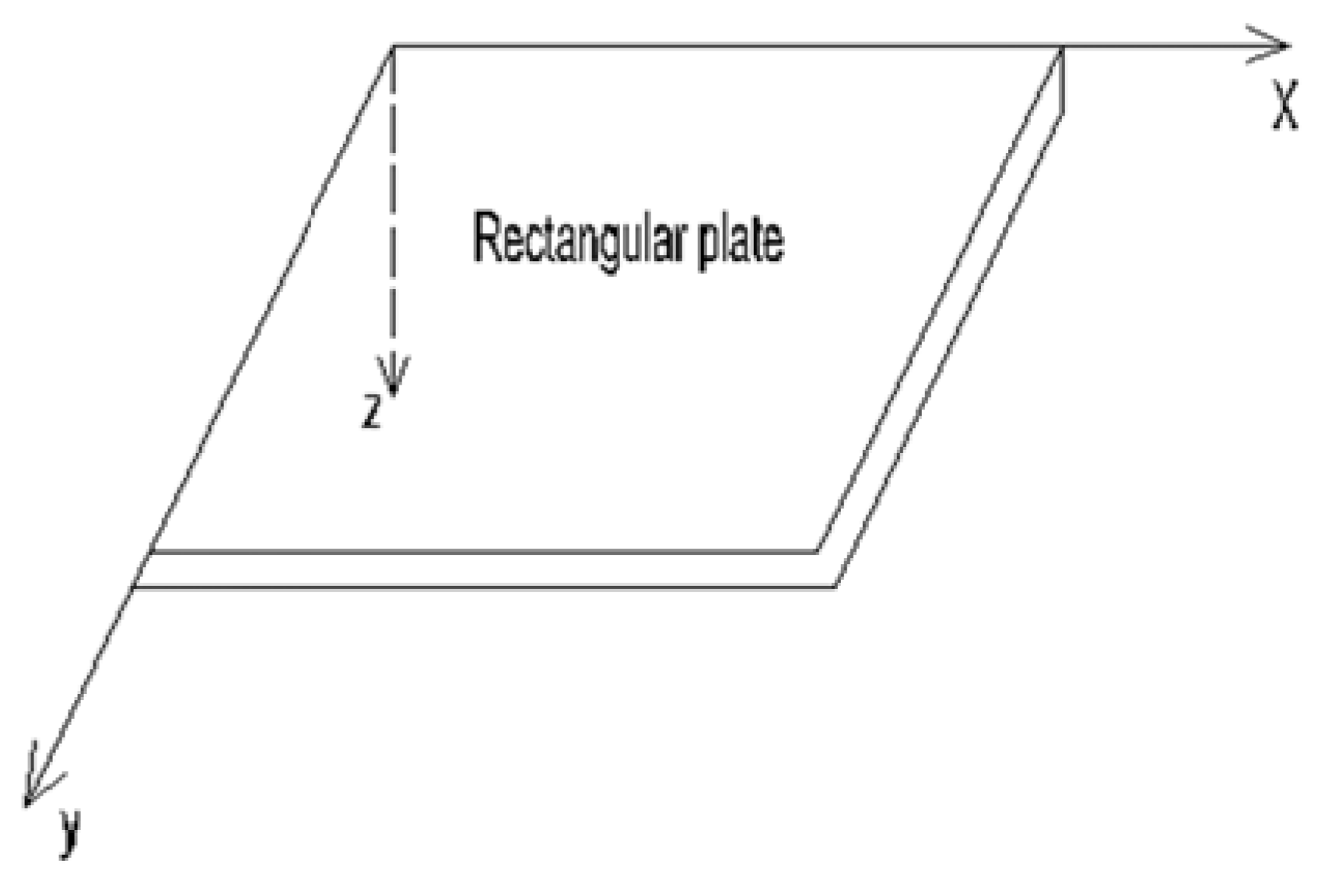
Figure 2.
a) Positions yi (●) in general b) Positions yi (●) for system symmetrical and loading symmetrical or anti symmetrical with respect to axis y = b/2.
Figure 2.
a) Positions yi (●) in general b) Positions yi (●) for system symmetrical and loading symmetrical or anti symmetrical with respect to axis y = b/2.
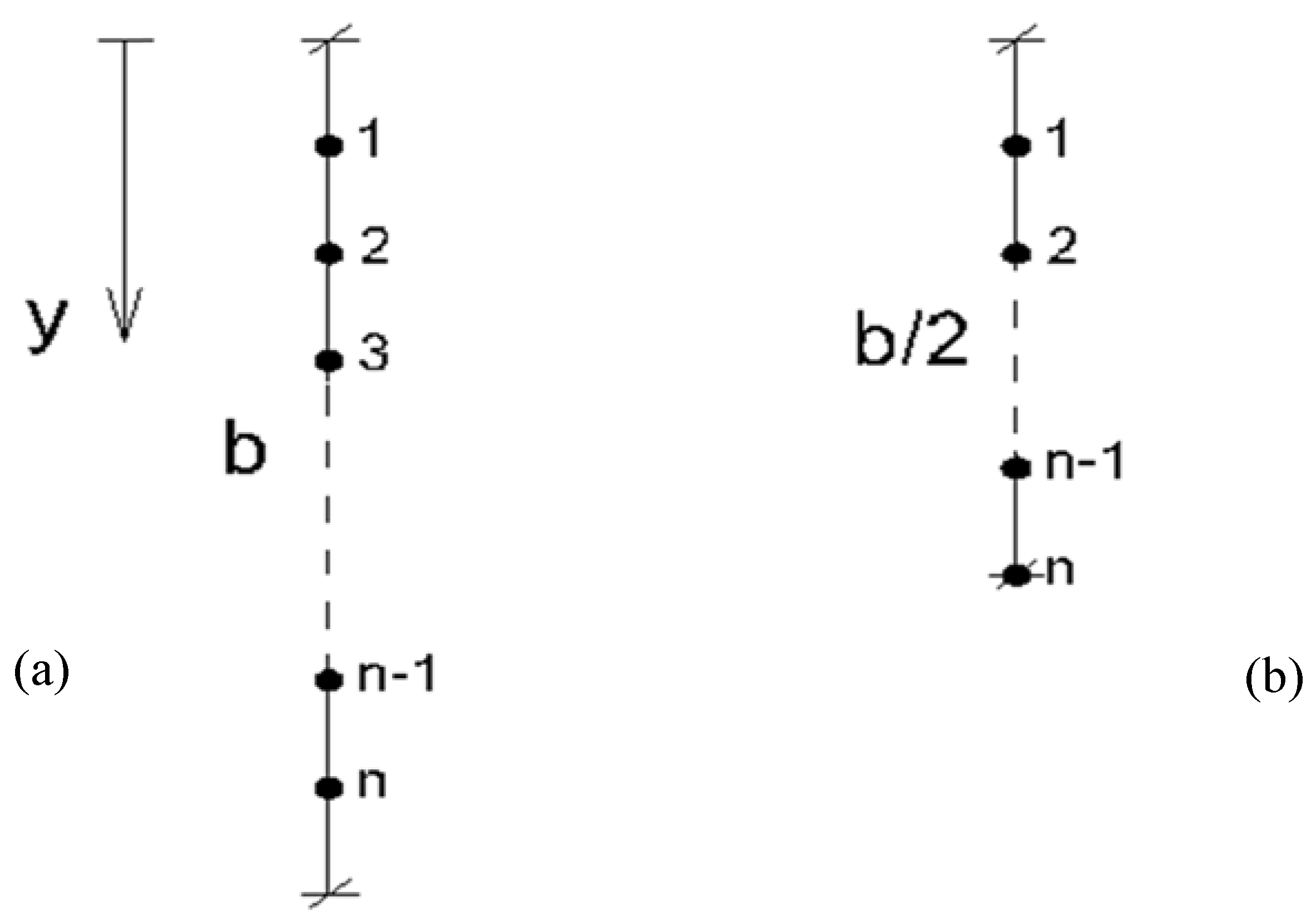
Figure 3.
Positions yi (●) for edges y = 0 supported and y = b free.
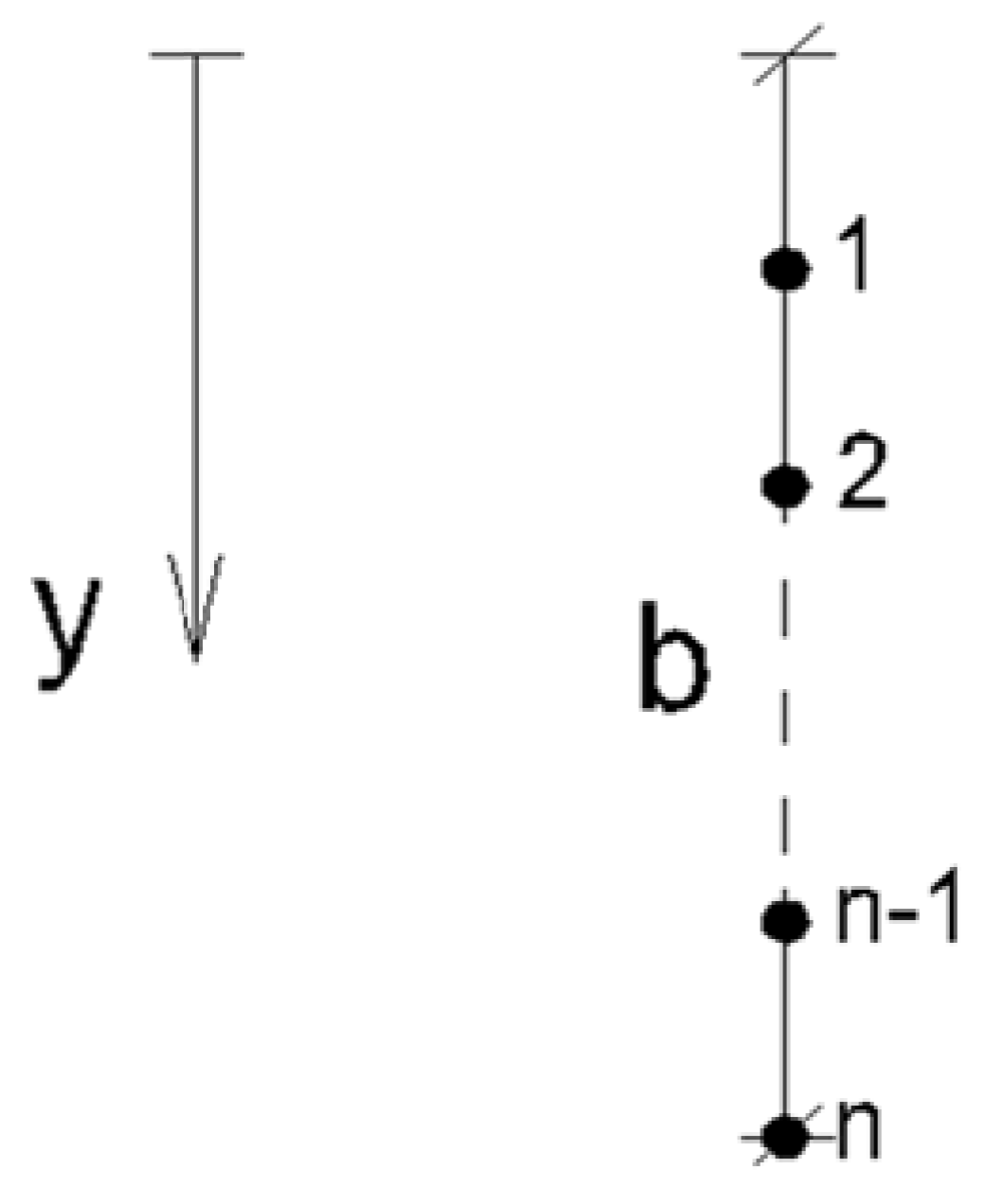
Figure 4.
a) Positions yi (●) in general b) Positions yi (●) for loading symmetrical or anti symmetrical with respect to axis y = b/2.
Figure 4.
a) Positions yi (●) in general b) Positions yi (●) for loading symmetrical or anti symmetrical with respect to axis y = b/2.
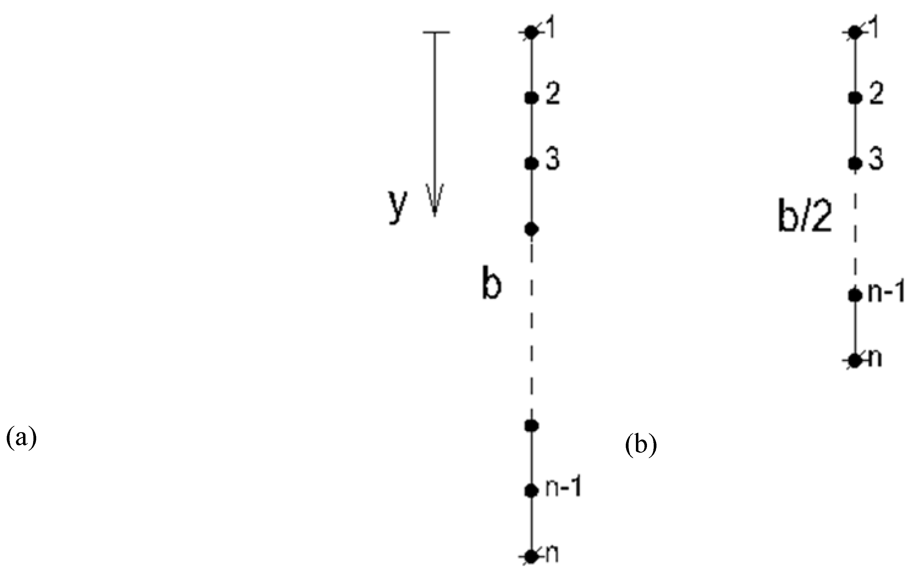

Table 1.
Coefficients of bending moments at the middle of the clamped edge and middle of the plate.
| b/a | 1.00 | 1.25 | ||||||
|---|---|---|---|---|---|---|---|---|
| Nx,cl | Nxm | Nym | Nx,cl | Nxm | Nym | |||
| Tables by Czerny[14] (exact results) | ||||||||
| 18.3 | 59.5 | 44.1 | 12.7 | 34.2 | 45.8 | |||
| Present study | ||||||||
| 1 redundant | 18.82 | 59.30 | 44.20 | 13.29 | 34.48 | 45.81 | ||
| 3 redundants | 18.29 | 59.31 | 44.03 | 13.03 | 34.34 | 45.74 | ||
| 5 redundants | 18.19 | 59.30 | 44.02 | 12.96 | 34.34 | 45.71 | ||
Table 2.
Coefficients of bending moments at the middle of the clamped edge and middle of the plate.
| b/a | 1.00 | 1.25 | |||||||
|---|---|---|---|---|---|---|---|---|---|
| Nx,cl | Ny,cl | Nxm | Nym | Nx,cl | Ny,cl | Nxm | Nym | ||
| Tables by Czerny[14] (exact results) | |||||||||
| 19.4 | 19.4 | 56.8 | 56.8 | 14.9 | 17.7 | 37.0 | 69.4 | ||
| Present study | |||||||||
| 1 redundant | 20.10 | 19.72 | 56.49 | 57.13 | 15.33 | 18.15 | 36.98 | 69.42 | |
| 3 redundants | 19.61 | 19.45 | 56.71 | 55.80 | 15.15 | 17.86 | 36.82 | 67.36 | |
Table 3.
Coefficients of bending moments at the clamped edge and at the middle of the plate.
| b/a | 1.00 | 1.20 | |||||||
|---|---|---|---|---|---|---|---|---|---|
| Nxm | Nym | Nx,frm | Nx,fre | Nxm | Nym | Nx,frm | Nx,fre | ||
| Tables by Czerny[14] (exact results) | |||||||||
| 21.42 | 79.85 | 16.60 | 7.89 | 27.91 | 143.64 | 23.29 | 11.40 | ||
| Present study | |||||||||
| 1 redundant | 20.92 | 70.85 | 16.21 | 7.69 | 26.56 | 116.24 | 22.44 | 10.85 | |
| 3 redundants | 21.42 | 79.89 | 16.61 | 7.97 | 27.89 | 144.74 | 23.28 | 11.41 | |
| 5 redundants | 21.40 | 79.77 | 16.59 | 7.90 | 27.87 | 143.53 | 23.27 | 11.40 | |
Disclaimer/Publisher’s Note: The statements, opinions and data contained in all publications are solely those of the individual author(s) and contributor(s) and not of MDPI and/or the editor(s). MDPI and/or the editor(s) disclaim responsibility for any injury to people or property resulting from any ideas, methods, instructions or products referred to in the content. |
© 2023 by the authors. Licensee MDPI, Basel, Switzerland. This article is an open access article distributed under the terms and conditions of the Creative Commons Attribution (CC BY) license (http://creativecommons.org/licenses/by/4.0/).
Copyright: This open access article is published under a Creative Commons CC BY 4.0 license, which permit the free download, distribution, and reuse, provided that the author and preprint are cited in any reuse.


