
Submitted:
16 May 2023
Posted:
17 May 2023
You are already at the latest version
Abstract
The intrinsic non-linearity and complexity of suspended sediment dynamics, which are impacted by the geographical variability of basin parameters and temporal climatic patterns, make it difficult to estimate suspended sediment concentration (SSC) accurately in hydrological processes. Deep neural networks (DNNs), a cutting-edge modeling method that can capture the innate non-linearity in hydrological systems, have emerged as a solution to this problem. Using primary data on discharge, SSC, and turbidity, the long short-term memory method of DNNs was employed in this study to simulate the discharge-suspended sediment connection for the Esopus Creek, NY, USA as the first objective. To develop effective modeling strategies, multiple scenarios of feature selection, including combinations of discharge, turbidity and SSC for preceding days, were considered. Secondly, the variations in SSC and discharge between the three USGS gages along Esopus Creek that were upper stream, lower stream, and downstream, adjacent to the pourpoint were analyzed. Statistical metrics and scenarios of feature importance were used to evaluate the effectiveness of the DNN-based models. The study shows that among 24 DNN approaches feature selection is crucial in simulating the daily SSC, and discharge and presenting novel research directions for utilizing machine learning algorithms in water quality.
Keywords:
Water quality
; suspended sediment
; discharge
; LSTM
; deep neural network
1. Introduction
Empirical techniques and the conventional sediment rating curve (SRC) have limited ability to forecast SSC. Sediment-filled rivers and streams present serious environmental and economic challenges [1]. Significant effects on a river’s channel morphology, material fluxes, geochemical cycling, water quality, and the biotic and aquatic ecosystems that rely on the river result from the delivery of suspended sediment concentration (SSC) by the river. Additionally, the geomorphological and biological processes of rivers are significantly impacted by fine silt, which has been found to be a key vector for the transportation of nutrients and contaminants [2]. Accurate assessment and long-term forecasting of sediment delivered by rivers are essential due to the possible consequences on biotic and aquatic habitats, as well as other land and water management processes [3]. Streamflow has been identified as the primary explanatory variable for SSC although it is not always directly related to SSC and that the relationship between the two is known to vary greatly [4,5,6]. The complexity of the sediment concentration transported hydrological phenomenon, which is a result of a number of ambiguous parameters including spatial variability of basin characteristics, river discharge patterns, and inherent non-linearity in hydro-meteorological parameters, is what primarily drives this variation [7]. Other factors to take into account are the availability of sediment, seasonality, and the location where the source resides within the watershed [8]. A streamflow hysteresis effect could also cause a significant fluctuation in SSC. The development of SSC prediction models has extensively utilized the variance in streamflow, which offers crucial information for the timing and changes in sediment concentrations. As measurements of suspended sediment in streams, turbidity, SSC, and TSS are all intricately related [1].
Simplified flow and sediment partial differential equations serve as the foundation for physical models. The models also rely on a number of erroneous flow-related simplification assumptions and actual connections for the effects of rainfall and flow erosion [9]. These models are incredibly intricate and complicated, with some of their components simulating actual physical processes. These models theoretically take into account the effects of geographical variation in watershed features as well as the uneven distribution of precipitation and evapotranspiration, according to prior studies [10,11]. Process-oriented distributed models are impractical because most of the variables are not currently measurable for much of the world. They have numerous drawbacks [12]. Numerical modeling is more relevant than analytical modeling since analytical approaches make basic assumptions [13]. However, it is sometimes hard to conduct numerical analyses of the transit of river-suspended silt under actual circumstances [14]. As a result, the feasibility of data-driven models as alternative methodologies for predicting SSC is commonly used. Data-driven (DD) models have an advantage over deterministic models in that they require fewer data and are better suited for forecasting. Kisi, 2012 argued that the ambiguity surrounding the internal structure of DD models was analogous to a ‘black box’ approach developed through a trial-and-error process. Despite their black-box nature, DD models are adaptable when it comes to capturing the nonlinearity of streamflow-sediment yield processes [9]. Due to its capacity to self-adapt, recognize patterns, and capture complicated non-linear behavior between input and output parameters, Deep Neural Network (DNN) has become an increasingly common modeling tool [15].
There are numerous examples of successful DNN applications in the field of water resources engineering. These include the prediction of variables such as sediment load [16,17,18,19,20,21,22], river flows [23,24,25,26,27,28], runoff [29,30,31,32,33], flood frequency analysis [34,35], flood forecasting [36,37] and streamflow data infilling procedures [38,39]. Joshi et al., 2016 used different combinations of input vectors (i.e., discharge, sediment, and stage) to develop a robust network model structure for simulating the discharge-sediment and stage-discharge-sediment relationships provide a more accurate estimate of SSC for the Bhagirathi River [3]. In their investigation, the performance of the generated DNN model simulations was evaluated using statistical parameters and compared to the results of the conventional sediment rating curve (SRC) approach. The DNN models outperformed the SRC technique in simulating the daily SSC according to the chosen performance indices. These results support the assertions made by scholars like Cigizoglu and Kisi (2005) regarding the use of streamflow, sediment concentration, and feed-forward back propagation (FFBP) algorithm inputs for daily or monthly SSC estimation and forecasting [40,41,42]. However, it has been reported that not enough studies have been conducted to evaluate the best performance of training algorithms within DNN modeling techniques [15]. The importance of training algorithm performance evaluation is emphasized by this argument, which notes that choosing the right algorithm is just as crucial as considering network architecture and shape. The research community will ultimately gain from the introduction of a mechanism for integrating predictive models into the cloud platform thanks to the usage of the neural network regression model in this study. The purpose of this study is to clarify the connections between SSC, turbidity and river discharge for Esopus Creek using deep neural network algorithms. The specific objectives of the study are to analyze the hidden patterns in the distribution of river discharge, SSC, and turbidity series, finding the feature importance and the most relevant features in prediction SSC and discharge downstream and implementing long short-term memory (LSTM) algorithms in predictions.
2. Materials and Methods
2.1. Study Location and Data Source
The Esopus Creek is a 105.3 km tributary of the Hudson River that drains the east-central Catskill Mountains in the U.S. state of New York, and its watershed covers 1,100 km2. Its source is Winnisook Lake, located on the slopes of Slide Mountain, and it flows to the Hudson River at Saugerties. As part of the water supply system for New York City, Esopus Creek is dammed at Olive Bridge halfway along its course to construct Ashokan Reservoir [43]. Additionally, 21 kilometers upstream of the reservoir, the creek’s water supply is augmented by water flow from the city’s Schoharie Reservoir. The Esopus is commonly referred to as two distinct streams of upper and lower stream with the Ashokan reservoir serving as the dividing point. The upper stream, which is frequented by recreational activities, exhibits traits of a typical mountain stream. The first studied USGS gage is located in the upper stream region of at mount Marion, NY. The latitude and longitude of the first gage (Gage 1- USGS 01362500) site are 42°00′52.1”, -74°16′12.7” with the coordinate system “North American Datum of 1983”, Ulster County, NY, Hydrologic Unit 02020006, 2.4 km upstream from Ashokan Reservoir with 497.3 km2 drainage area and the datum of gage of 189.24 m above NAVD of 1988 [44].
The Lower Esopus region is defined from Ashokan Reservoir to Kingston where the second selected USGS gage (Gage 2- USGS 01363556) is located. The latitude and longitude of the second gage site are 41°52’45.6”, -74°08’43.3” with the 9 km distance to the downstream from Ashokan Reservoir, the drainage area of 722.6 km2 and gage datum of 58.2 m above NAVD of 1988 [45]. Before Esopus Creek meets the Hudson River, the third USGS gage (Gage 3- USGS 01364500) is located along Esopus Creek’s last section, approximately 10 kilometers from Kingston to Saugerties. The latitude and longitude of the third gage site are 42°02′16”, -73°58′19” with 7 km distance to the upstream of Saugerties (adjacent to Hudson River), the drainage area of 1,085 km2 and gage datum of about 12 m above NAVD of 1988 [46]. Table 2 listed the USGS gages used in the study with maximum discharge for the last year and highest peak discharge for the last five years [47].

Table 1.
Study locations and data sources.
| Gage | Location | Max. discharge (last 365 days) (m3/s) | Highest peak discharge (m3/s) |
|---|---|---|---|
| USGS 01362500 | Esopus Creek at Coldbrook, NY- Upper Esopus region | 450.2 | 2146.4 |
| USGS 01363556 | Esopus Creek near Lomontville, NY- Lower Esopus region | 117.2 | 191.7 |
| USGS 01364500 | Esopus Creek at mount Marion, NY- Downstream (adjacent the Hudson River) | 314.3 | 863.7 |
Esopus Creek flow path illustrated in Figure 1 using the USGS Streamer website to locate the upstream and downstream of the Creek meeting the Hudson River eventually with the location of streamflow-gauging stations [48,49].
The Esopus Creek is a tributary of the Esopus Creek, eventually emptying into the Ashokan Reservoir, which supplies approximately 10% of NYC’s drinking water (GCSWCD) [50]. The landscape, valleys, and stream channel shape are all clearly influenced by the Catskill Mountains’ geology. The U.S. Geological Survey maintains a streamflow-gauging station on Esopus Creek that provides a continuous discharge record, SSC, and turbidity for three locations along the flow path until it reaches to the Hudson River.
The data availability for each gage location is different due to the USGS data source and data collection. Although, the SSC is available since 10/01/2016 and 9/11/2013 at gage 1 and gage 3, respectively as the main parameter focused on this study, the analysis duration is limited to the data availability at gauge 2. Hence, the comparison conducted based on the date ranges between 2/28/2020 and 9/30/2021.
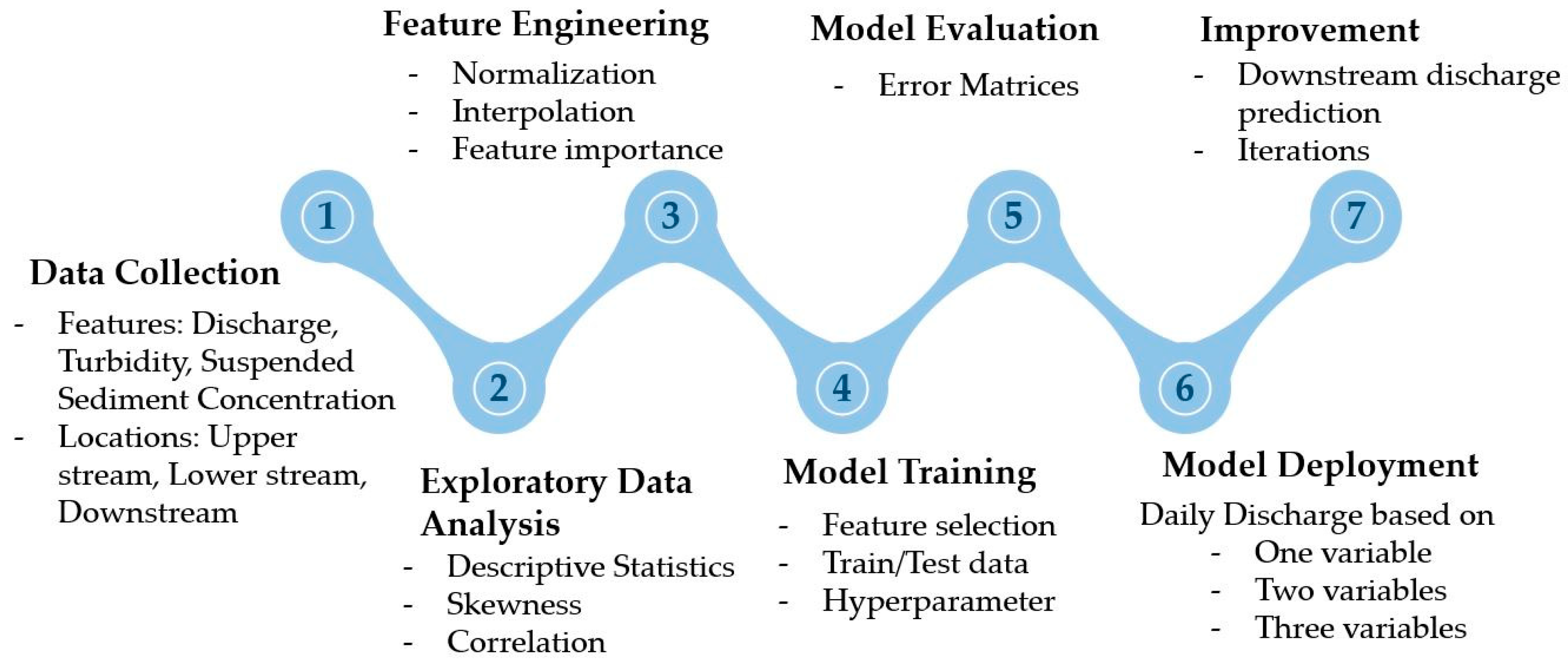
The overall workflow consists of seven main steps, starting with data collection, Exploratory Data Analysis (EDA), Feature Engineering (FE), and then model training, evaluation, deployment and improvement. The first steps, data collection from the USGS website, an exploratory analysis of three variables, and feature engineering are conducted on all three locations to identify the feature importance and their ranking in SSC and discharge prediction at the lower end stream location. Then the combined dataset of all three sites transforms the data for model training and testing to a subset of data and performs the LSTM analysis. Variables are listed in Table 2. as features studied in this research. After investigating the dataset and performing data transformation on the variables, LSTM neural network is trained using the data prepared in the initial steps to perform predictive analysis. LSTM neural networks regression model is assessed using several error matrices (e.g., Root Mean Square Error (RMSE), and Mean Absolute Error (MAE)). for better accuracy.
To reduce prediction errors and achieve sufficient performance, the LSTM algorithm is adjusted and improved through modifying the hyperparameters. The LSTM prediction is deployed on two main strategies. The first strategy mainly focusses on predicting the downstream discharge and the second strategy involved with predicting the SSC at the downstream based on the most relevant features modified in by feature importance analysis. Model performance is further improved through iterative incorporation and validation of the input variables. The LSTM workflow of predicting both discharge and SSC is shown in Figure 2
Figure 2.
LSTM prediction workflow.
The time series of the discharge, SSC, and turbidity variables are obtained from the USGS National Water Information System in the first step of the workflow in Figure 2 [51]. The range of the time series data for all the variables was different due to the various recorded duration. The similar range of data that all the nine features were available used in this research is from 2/28/2020 to 9/30/2021. The time-series data has daily recording. Table 1 represent the variables recorded for the three USGS locations used in the study.
Table 2.
List of the variables used for EDA and predictive analysis with LSTM model.
| SW Parameters | Unit | Descriptions |
|---|---|---|
| Discharge | m3/s | Quantity of stream flow |
| Turbidity | FNU (Forest technology systems) | Water quality parameter that refers to how clear the water is |
| Suspended Sediment Concentration | mg/L | The proportion of the weight of sediment that is dry in a mixture of water and sediment, relative to the total weight of the mixture. |
2.2. Multivariate Exploratory Data Analysis
A detailed Exploratory Data Analysis (EDA) is performed in Figure 3 activity 2 to understand the attributes and characteristics of the multivariate dataset [52]. To achieve satisfactory LSTM model performance, exploratory data analysis (EDA) is a crucial stage in completing preliminary data analyses. The internal temporal distribution of these three variables is investigated using a variety of visual and numerical indices. EDA is the process of conducting a preliminary analysis of the input variables to comprehend the hidden pattern of the variables’ distribution. Activities constitute an additional component of EDA. These include identifying outliers and extreme numbers, as well as performing a normality check. Descriptive statistics is an excellent method for determining the distribution of the values of input variables based on the number of data points, mean, standard deviation, percentiles, interquartile range, and range. Table 3 displays full multivariate descriptive statistics.
Histograms with density plots are used as a visual representation of normality in the variables, and Pearson’s coefficient of skewness (PCS) is used as a numerical indicator of skewness. Figure 3 depicts a visual representation of the distribution of the input variables, indicating that the overall non-normality is high. The legend of each plot shows the skewness values. All variables exhibit significant non-normality and skewness. PCS values of turbidity and SSC related to discharge and skewness of all three variables are indicated as a numerical measure of non-normality/skewness.
Figure 4 illustrates that the linear connection between turbidity and discharge variables is higher than the linear relationship between SSC and discharge values. Lower values of the linear coefficients to delineate the overall non-linearity among several variables is high. The direction of the linear relationships is found to be positive in both turbidity and SSC with more weight on turbidity relative to discharge. The high linear relationship between SSC and turbidity among all three locations are vividly obvious throughout the correlation coefficient. While there might be non-linear relationship between SSC and discharge values, the LSTM prediction assists the higher correlation via prediction. The feature engineering in the next section calculated the feature importance and their ranking in predicting either SSC_3 and discharge_3.
2.3. Feature Engineering
After an effective initial analysis of the dataset using EDA, feature engineering (FE) is carried out. The LSTM approach may not yield adequate results with little error if the FE is unsuccessful. Iterative gradient descent optimization cannot be effective without an appropriate set of data analysis. The variables that are most suitable for the LSTM learning algorithm are therefore transformed through substantial feature engineering. In this study, FE is used to perform imputation, data transformation, data normalization, and dataset segmentation into training, and testing sets. Linear interpolation is used to fill in the null values to make the entire dataset consistent. Sensor malfunctions resulted in null values or observations in every series. In the combined dataset including all three USGS gages, there were 19, 2, and 1 missing values for turbidity, SSC and discharge at USGS 01362500 respectively. There were only 6 missing values for turbidity and SSC and at USGS 01363556 and there were 16 missing values for turbidity and SSC and at USGS 01364500.
Data normalization is the process used to obtain each variable’s values prepared for additional analysis and using the DNN algorithm. All the variables are scaled to values with a mean of zero and a variation of one as part of the normalizing procedure. The entire normalized variable series is divided into two sections a training set that is used to train the model and a testing set that is used to evaluate the model. In this study the training and testing sets consist of 70 percent and 30 percent of the dataset, which is 551, 367, and 184 number of observations, training observations, testing observations points.
Firstly, a trained random forest model in Scikit-Learn’s (rf.feature_importances (RFE)) property outputs an array of feature importance scores. Based on each feature’s success in reducing impurity in the random forest’s decision trees, the feature’s importance scores are determined. The higher the feature importance score, the more significant the feature is for the prediction. Conducting feature importance analysis on the study dataset resulted in feature importance scores of 0.0069, 0.0070, 0.3534, 0.0125, 0.0139, 0.5301, 0.0324, and 0.0439 for Turbidity_1, SSC_1, Discharge_1, Turbidity_2, SSC_2, Discharge_2, Turbidity_3, and SSC_3, respectively to predict Discharge_3. This indicates that ‘Discharge_2’, ‘Discharge_1’, ‘SSC_3’, ‘Turbidity_3’, ‘SSC_2’, ‘Turbidity_2’, ‘SSC_1’, and ‘Turbidity_1’ are the most important features in predicting Discharge_3, respectively. Hence, Prediction of discharge values at the downstream (Discharge_3) is mainly correlated with the discharge values at the upper stream and lower stream. Suspended sediment concentration in all three locations showed higher correlated values than turbidity. Hence selecting the lower number of features rather than all of them is the next step in optimizing model prediction.
Secondly, in Recursive Feature Elimination (RFE), the least significant features are repeatedly removed from the dataset until the desired number of features is obtained. RFE is a backward feature selection technique. The process begins with the model being fitted to the entire dataset, followed by a ranking of the features by importance using a particular metric, the removal of the least important feature, and fitting the model again on the remaining features. The procedure is continued up until the desired number of characteristics is attained. The random forest regressor model on the time series dataset, performs RFE with a target of selecting 5 features, and output the ranking of all features in the dataset. The top-ranked features can be selected in prediction model. Having an assumption of selecting 4 features by RFF indicated ‘Discharge_1′, ‘Discharge_2′, ‘Turbidity_3′, and ‘SSC_3′ the most relevant features. Dropping the discharged values allowed the RFF decision to be made on only turbidity and SSC at three locations and resulted in the features shown in Table 3.
Table 3.
Recursive Feature Elimination (RFE) results for the most relevant features to predict discharge downstream.
Table 3.
Recursive Feature Elimination (RFE) results for the most relevant features to predict discharge downstream.
| Selection among | Most relevant features |
|---|---|
| All features | ‘Discharge_1′, ‘Discharge_2′, ‘Turbidity_3′, ‘SSC_3′ |
| Dropping discharges’ values | |
| 4 top features | ‘Turbidity_2’, ‘SSC_2’, ‘Turbidity_3’, and ‘SSC_3’ |
| 3 top features | ‘Turbidity_2’, ‘SSC_2’, and ‘SSC_3’ |
| 2 top features | ‘Turbidity_2’, and ‘SSC_3’ |
| 1 top feature | ‘SSC_3’ |
Main focus of this study is the suspended sediment concentration prediction which allow the resultant algorithm to anticipate the critical range of SSC especially at the downstream location correlated to water quality standards. The same procedure was made on the dataset in terms of feature importance and having the SSC_3 as target variable. The random forest feature importance analysis on SSC_3 prediction evaluated ‘SSC_1’, ‘SSC_2’, ‘Turbidity_3’, and ‘Turbidity_2’ as the most important features, respectively. RFE ranked the most relevant features that are shown in Table 4 based on the number of selected features. Based on bivariate correlation coefficients results discussed earlier the turbidity values represent the same pattern and behavior as SSC. Hence, dropping turbidity values made the important feature selection focused on discharge and SSC values.
2.4. Long Short-Term Memory (LSTM) Recurrent Neural
LSTM has come to be a favorite method for analyzing time series data in deep learning forecasting, where variables depend on prior historical knowledge throughout the data series. LSTM can be used to identify the long-term correlations and linkages between the variables. Recur-rent backpropagation demands a large amount of computational time and effort to learn to store long-term knowledge because of the decaying error backflow. Hence, the concept of the vanishing gradient problem in recognizing long-term dependency of Recurrent Neural Network (RNN) was introduced [42,53]. The main element of processing and retaining long-term information is LSTM feedback connections, and this characteristic distinguishes it from the conventional feedforward neural network. Both long-term memory (c[t-1]) and short-term memory (h[t-1]) are processed in a typical LSTM algorithm through the utilization of multiple gates to filter the information. For an unchanged flow of gradients, forget and update gates update the memory cell state. Three gates i.e., input gate ig, forgot gate fg, output gate og and cell state handle the information flow by writing, deleting, preserving past information, and reading respectively (Figure 2). LSTM has applications for time series prediction inside a specified window since it can memorize data at varying lead times.
Figure 2.
A Schematic LSTM structure.

In this research, a neural network with one LSTM hidden unit accompanied by a dense layer connecting the LSTM target output at the last time-step (t-1) to a single output neuron with non-linear activation function. The LSTM model was trained using the deep learning library, Keras in Python, and the RMSE, and MAE [54,55,56,57,58]. To predict the discharge variable of a time-step in the future daily values of the variables at the previous time-steps are used. Hyperparameters are tuned to maximize the performance of the LSTM model through an iterative trial-and-error approach. In this study, Keras, a python library that offers a space search for machine learning algorithms is used to find the best combination of the hyperparameters [59]. Considered hyperparameter of the LSTM algorithm in this study is the size of epoch, batch size, dropout rate, and number of neurons.
2.5. Prediction Scenarios
The dataset has daily intervals for all the variables and the time series analysis by LSTM conducted on daily for prediction Based on the feature importance ranking in Table 3 and 4 for discharge and SSC prediction, three scenarios selected for each target variable among discharge and SSC separately. The study focuses on the accuracy of predicting discharge downstream based on the most relevant features among SSC and turbidity for the first round of analysis. Secondly, the LSTM accuracy in predicting SSC based on most relevant features of discharge and turbidity studied. All trials run based on the maximum 4 days (steps) forward as time lead considering 1 most relevant feature, 3 most relevant features and all variables. This series of analysis resulted in sensitivity analysis on feature importance and selection.
The resultant prediction can indicate the importance and sensitivity of prediction based on the resolution of the input data. The comparison between these scenarios demystifies the improvement of discharge and SSC prediction considering available features.
2.6. Model Evaluation Using Loss Functions
The top two standard error matrices, such as RMSE and MAE, are used to assess the performance of the LSTM model. By comparing the observed and predicted values, error matrices provide numerical numbers as a measure of the performance of the model. The LSTM model is assessed using the RMSE value to demonstrate model performance enhancement. The squared term exponentially amplifies larger errors more than smaller ones, putting the RMSE as a function more vulnerable to larger errors. The best predicted accuracy is correlated with the lowest RMSE score.
3. Results and Discussion
This LSTM neural network is used to predict the multivariate turbidity, SSC, and discharge daily variables based on the previous time series data. The prediction values of 1, 2, 3, and 4 (days) lead time chosen for both scenarios with the fixed time lag of 30 previous steps to be consistent with various LSTM models. Predicted values are compared to the observed dataset to quantify the error matrices. The RMSE, and MAE, are used to estimate the error from the predicted discharge, SSC, and turbidity variables. The model performance is improved by an increase in the number of epochs. Error matrices are obtained through multiple models runs to demonstrate the linkage between the model performance and the lead times.
3.1. Model Evaluation Matrices and Predictions Comparison
The output from the LSTM algorithm is compared to the observed values of the discharge, SCC, and turbidity variables and two main error metrices of RMSE and MAE calculated on each scenario. Figure 6 represents 3 main scenarios results in two series of considering SSC_3 and Discharge_3 as target variable. Figure 6, (a) is the first scenario based on selecting the most important feature in predicting SSC_3 discussed in Table 4 (‘SSC_2’). Similarly, the first scenario on prediction the ‘Discharge_3′ represented in Figure 6 (b) considering the importance of features based on Table 3 (SSC_3). Second scenarios represented in Figure 6 (c), and (d) for SSC_3 and Discharge_3 prediction respectively. The selected features for SSC_3 prediction by top three relevant features after discarding turbidity values which are ‘SSC_2′, ‘Discharge_3’, and ‘Discharge_1’. Discharge_3 prediction for second scenarios conducted by considering ‘Turbidity_2’, ‘SSC_2’, and ‘SSC_3’ and results represented in Figure 6 (d).
The third scenario considered the four most relevant features among all features for both SSC_3 and discharge_3 prediction based on Table 3 and Table 4 which the results presented in Figure 6, (e) and (f).
The least RMSE values reported consistency in all trials with the lower lead time of 1 day as a common result. The closer the lead time to the current observed values, the highest accuracy potentially achieved. The best accuracy considering the lowest error of RMSE and MAE for SSC_3 prediction recorded by Scenario 3 and considering 4 most relevant features (‘Turbidity_3’, ‘Turbidity_1’, ‘Discharge_3’, ‘SSC_1’) as 23.041 and 12.874, respectively. Whereas the highest accuracy of Discharge_3 prediction in all scenarios results from the second scenario considering one most relevant feature (‘SSC_3’) for 2 days lead time based on minimum RMSE values of 19.962 and 1 day lead time based on minimum MAE value of 13.881.
3.2. Model Improvement
The performance of the model was also evaluated and improved by running hyperparameter analysis on multiple parameters in LSTM model such as ‘batch size’, ‘dropout rate’, ‘epochs’, and ‘number of neurons’ for all scenarios. Increasing the number of iterations i.e., epoch in the neural network could not always improve the model performance the same as increasing the number of neurons, dropout rate and batch size in all the algorithm and scenarios Hyperparameter feature allows each run to be freely select the parameters of the LSTM network that results in a lowest error. Selection of parameters is made among the range of [2, 10, 20, 30] for number of neurons, [0.1, 0.2, 0.3] for dropout rate, [50, 150] number of epochs and [64, 128] batch sizes.
For the first scenario of having SSC_3 as target variable the hyperparameter results in ‘batch size’: 128, ‘dropout rate’: 0.1, ‘epochs’: 150, and ‘number of neurons’: 10. Having Discharge_3 as target variable results ‘batch size’: 128, ‘dropout rate’: 0.1, ‘epochs’: 50, and ‘number of neurons’: 2. In the second scenario, SSC_3 target variable results in ‘batch size’: 128, ‘dropout rate’: 0.1, ‘epochs’: 50, and ‘number of neurons’: 10, whereas the Discharge_3 target variable adjusted ‘batch size’: 128, ‘dropout rate’: 0.3, ‘epochs’: 50, and ‘number of neurons’: 2. Lastly the hyperparameter tunning of the third scenario for SSC_3 prediction reported ‘batch size’: 128, ‘dropout rate’: 0.1, ‘epochs’: 50, and ‘number of neurons’: 20. The Discharge_3 prediction in the third scenario results in having ‘batch size’: 64, ‘dropout rate’: 0.1, ‘epochs’: 50, and ‘number of neurons’: 2 as best parameters. Hence, even by having the same dataset, and target variable, the feature selection based on their ranking impact the best parameters for LSTM network in obtaining highest accuracy model.
4. Conclusion
Although many rivers have the potential to be SSC sources, it is essential to quantify sediment concentration accurately in order to understand how it relates to water outflow for the planning and management of water resources. in this study, DNN algorithms is used to investigate the importance of feature selection in forecasting SSC and downstream discharge across three locations in Esopus Creek. With a focus on taking into account hyperparameters that optimize the LSTM network model, our findings showed that the significance of each feature differs in predicting the target variables. The conclusions of these analyses showed that choosing features with the greatest importance was successful in producing accurate predictions. Discharge, SSC, and turbidity are the three main water quantity and quality parameters in the river in this study.
For simulation, primary data of discharge, SSC, and turbidity for the period from 2/8/2020 to 9/30/2021 are used. Combinations of various features based on their importance and ranking in three main scenarios considered.
Daily times-series values of discharge, SSC, and turbidity were utilized as input, and model simulations were run using a distinct set of input combinations. RMSE, and MAEwere used to test the performance of the LSTM model simulations.
In general, hysteresis generated by LSTM simulations captures nonlinear dynamics, generalizes the structure of the entire data set and performs well with observed sediment concentration series data. As a result, the study suggests that conducting feature importance and the correlation between each variable depends on the target variable that needs to be taken into account prior to any DNN algorithms simulation. Hyperparameter analysis also is a vital task in DNN prediction as the results show the variety of network parameters selection are available and only one in each scenarios revealed to produce the highest accuracy.
Consequently, this study presents novel research opportunities for improving other DNN algorithms and integrating hybrid soft computing techniques to enhance the accuracy of short- and long-term predictions of SSCs in water discharge. The findings of this research hold particular significance for water resource management projects in the southeast region of New York, as they shed light on sediment flux dynamics in both upstream and downstream areas. The insights gained from this study will contribute to more effective management of water resources in other regions as well.
Author Contributions
Conceptualization, S. G., M.K. and N. N.; methodology, S. G., M.K. and N. N.; software, M.K.; validation, S. G., M.K. and N. N.; formal analysis, M.K.; investigation, N.N.; resources, S. G. and N. N.; data curation, S. G., M.K. and N. N.; writing—original draft preparation, S. G. and N. N. N.; writing—review and editing, M.K., and N.N.; visualization, M.K.; supervision, M.K., S.G; project administration, N.N.; All authors have read and agreed to the published version of the manuscript.
Funding
This research received no external funding.
Institutional Review Board Statement
Not applicable.
Data Availability Statement
Data collected for the study can be made available upon request from the corresponding author.
Conflicts of Interest
The authors declare no conflict of interest.
References
- USGS Surface-Water Data for Minnesota. Available online: https://waterdata.usgs.gov/mn/nwis/sw (accessed on 17 November 2022).
- Caroni, E.; Singh, V.P.; Ubertini, L. Rainfall-Runoff-Sediment Yield Relation by Stochastic Modelling. Hydrol. Sci. J. 1984, 29, 203–218. [Google Scholar] [CrossRef]
- Joshi, R.; Kumar, K.; Adhikari, V.P.S. Modelling Suspended Sediment Concentration Using Artificial Neural Networks for Gangotri Glacier. Hydrol. Process. 2016, 30, 1354–1366. [Google Scholar] [CrossRef]
- Tornes, L.H. Suspended Sediment in Minnesota Streams; Water-Resources Investigations Report; U.S. Geological Survey: St. Paul, MN, 1986; Vol. 85–4312; [Google Scholar]
- Tornes, L.H.; Brigham, M.E.; Lorenz, D.L. Nutrients, Suspended Sediment, and Pesticides in Streams in the Red River of the North Basin, Minnesota, North Dakota, and South Dakota, 1993-95; Water-Resources Investigations Report; U.S. Geological Survey: Mounds View, MN, 1997; Vol. 97–4053. [Google Scholar]
- Blanchard, R.A.; Ellison, C.A.; Galloway, J.M. Sediment Concentrations, Loads, and Particle-Size Distributions in the Red River of the North and Selected Tributaries near Fargo, North Dakota, during the 2010 Spring High-Flow Event. 36.
- Fleming, G.; Harrison, A.; Fleming, J.; Kite, G.; Chitale, S.; Herbertson, J.; Collins, M. Discussion. Design Curves for Suspended Load Estimation. Proc. Inst. Civ. Eng. 1970, 46, 81–92. [Google Scholar] [CrossRef]
- Knighton, D. Fluvial Forms and Processes: A New Perspective; 2nd ed.; Routledge: London, 1998; ISBN 978-0-203-78466-2. [Google Scholar]
- Kisi, O. Modeling Discharge-Suspended Sediment Relationship Using Least Square Support Vector Machine. J. Hydrol. 2012, 456–457, 110–120. [Google Scholar] [CrossRef]
- Wicks, J.M.; Bathurst, J.C. SHESED: A Physically Based, Distributed Erosion and Sediment Yield Component for the SHE Hydrological Modelling System. J. Hydrol. 1996, 175, 213–238. [Google Scholar] [CrossRef]
- Refsgaard, J.C. Parameterisation, Calibration and Validation of Distributed Hydrological Models. J. Hydrol. 1997, 198, 69–97. [Google Scholar] [CrossRef]
- Tayfur, G.; Guldal, V. Artificial Neural Networks for Estimating Daily Total Suspended Sediment in Natural Streams. Hydrol. Res. 2006, 37, 69–79. [Google Scholar] [CrossRef]
- Bor, A. Numerical Modeling of Unsteady and Non-Equilibrium Sediment Transport in Rivers | PDF | Fluid Dynamics | Water Resources Available online:. Available online: https://www.scribd.com/document/143503869/t-000755 (accessed on 17 November 2022).
- Salih, S.Q.; Sharafati, A.; Khosravi, K.; Faris, H.; Kisi, O.; Tao, H.; Ali, M.; Yaseen, Z.M. River Suspended Sediment Load Prediction Based on River Discharge Information: Application of Newly Developed Data Mining Models. Hydrol. Sci. J. 2020, 65, 624–637. [Google Scholar] [CrossRef]
- Mustafa, M.R.; Rezaur, R.B.; Saiedi, S.; Isa, M.H. River Suspended Sediment Prediction Using Various Multilayer Perceptron Neural Network Training Algorithms—A Case Study in Malaysia. Water Resour. Manag. 2012, 7, 1879–1897. [Google Scholar] [CrossRef]
- Kerem Cigizoglu, H.; Kisi, Ö. Methods to Improve the Neural Network Performance in Suspended Sediment Estimation. J. Hydrol. 2006, 317, 221–238. [Google Scholar] [CrossRef]
- Alp, M.; Cigizoglu, H.K. Suspended Sediment Load Simulation by Two Artificial Neural Network Methods Using Hydrometeorological Data. Environ. Model. Softw. 2007, 22, 2–13. [Google Scholar] [CrossRef]
- Kisi, Ö. Constructing Neural Network Sediment Estimation Models Using a Data-Driven Algorithm. Math. Comput. Simul. 2008, 79, 94–103. [Google Scholar] [CrossRef]
- Jothiprakash, V.; Garg, V. Reservoir Sedimentation Estimation Using Artificial Neural Network. J. Hydrol. Eng. 2009, 14, 1035–1040. [Google Scholar] [CrossRef]
- Kisi, O.; Haktanir, T.; Ardiclioglu, M.; Ozturk, O.; Yalcin, E.; Uludag, S. Adaptive Neuro-Fuzzy Computing Technique for Suspended Sediment Estimation. Adv. Eng. Softw. 2009, 40, 438–444. [Google Scholar] [CrossRef]
- Chou, W.-C. Modelling Watershed Scale Soil Loss Prediction and Sediment Yield Estimation. Water Resour. Manag. 2010, 24, 2075–2090. [Google Scholar] [CrossRef]
- Guven, A.; Kişi, Ö. Estimation of Suspended Sediment Yield in Natural Rivers Using Machine-Coded Linear Genetic Programming. Water Resour. Manag. 2011, 25, 691–704. [Google Scholar] [CrossRef]
- Smith, J.; Eli, R.N. Neural-Network Models of Rainfall-Runoff Process. J. Water Resour. Plan. Manag. 1995, 121, 499–508. [Google Scholar] [CrossRef]
- Tawfik, M.; Ibrahim, A.; Fahmy, H. Hysteresis Sensitive Neural Network for Modeling Rating Curves. J. Comput. Civ. Eng. 1997, 11, 206–211. [Google Scholar] [CrossRef]
- PANAGOULIA, D. Artificial Neural Networks and High and Low Flows in Various Climate Regimes. Hydrol. Sci. J. 2006, 51, 563–587. [Google Scholar] [CrossRef]
- Fernando, D.A.; Shamseldin, A.Y. Investigation of Internal Functioning of the Radial-Basis-Function Neural Network River Flow Forecasting Models. J. Hydrol. Eng. 2009, 14, 286–292. [Google Scholar] [CrossRef]
- Edossa, D.C.; Babel, M.S. Application of ANN-Based Streamflow Forecasting Model for Agricultural Water Management in the Awash River Basin, Ethiopia. Water Resour. Manag. 2011, 25, 1759–1773. [Google Scholar] [CrossRef]
- Kisi, O.; Nia, A.; Gosheh, M.; Tajabadi, M.; Ahmadi, A. Intermittent Streamflow Forecasting by Using Several Data Driven Techniques. Water Resour. Manag. Int. J. Publ. Eur. Water Resour. Assoc. EWRA 2012, 26, 457–474. [Google Scholar] [CrossRef]
- Shamseldin, A.Y. Application of a Neural Network Technique to Rainfall-Runoff Modelling. J. Hydrol. 1997, 199, 272–294. [Google Scholar] [CrossRef]
- Jayawardena, A.W.; Fernando, D.A.K. Use of Radial Basis Function Type Artificial Neural Networks for Runoff Simulation. Comput.-Aided Civ. Infrastruct. Eng. 1998, 13, 91–99. [Google Scholar] [CrossRef]
- Ju, Q.; Yu, Z.; Hao, Z.; Ou, G.; Zhao, J.; Liu, D. Division-Based Rainfall-Runoff Simulations with BP Neural Networks and Xinanjiang Model. Neurocomputing 2009, 72, 2873–2883. [Google Scholar] [CrossRef]
- Bhadra, A.; Bandyopadhyay, A.; Singh, R.; Raghuwanshi, N.S. Rainfall-Runoff Modeling: Comparison of Two Approaches with Different Data Requirements. Water Resour. Manag. 2010, 24, 37–62. [Google Scholar] [CrossRef]
- Evsukoff, A.G.; Lima, B.S.L.P. de; Ebecken, N.F.F. Long-Term Runoff Modeling Using Rainfall Forecasts with Application to the Iguaçu River Basin. Water Resour. Manag. 2011, 25, 963–985. [Google Scholar] [CrossRef]
- Kordrostami, S.; Alim, M.A.; Karim, F.; Rahman, A. Regional Flood Frequency Analysis Using an Artificial Neural Network Model. Geosciences 2020, 10, 127. [Google Scholar] [CrossRef]
- Hall: Regional Flood Frequency Analysis Using Artificial... - Google Scholar Available online:. Available online: https://scholar.google.com/scholar_lookup?title=Regional%20Flood%20Frequency%20Analysis%20Using%20Artificial%20Neural%20Networks&publication_year=1998&author=M.J.%20Hall&author=A.W.%20Minns (accessed on 17 November 2022).
- Karl, A.K.; Lohani, A.K. Development of Flood Forecasting System Using Statistical and ANN Techniques in the Downstream Catchment of Mahanadi Basin, India. J. Water Resour. Prot. 2010, 2, 880–887. [Google Scholar] [CrossRef]
- Kar, A.K.; Winn, L.L.; Lohani, A.K.; Goel, N.K. Soft Computing–Based Workable Flood Forecasting Model for Ayeyarwady River Basin of Myanmar. J. Hydrol. Eng. 2012, 17, 807–822. [Google Scholar] [CrossRef]
- Khalil, M.; Panu, U.S.; Lennox, W.C. Groups and Neural Networks Based Streamflow Data Infilling Procedures. J. Hydrol. 2001, 241, 153–176. [Google Scholar] [CrossRef]
- Mehedi, M.A.A.; Yazdan, M.M.S.; Ahad, M.T.; Akatu, W.; Kumar, R.; Rahman, A. Quantifying Small-Scale Hyporheic Streamlines and Resident Time under Gravel-Sand Streambed Using a Coupled HEC-RAS and MIN3P Model. Eng 2022, 3, 276–300. [Google Scholar] [CrossRef]
- Cigizoglu, H.K.; Kişi, Ö. Flow Prediction by Three Back Propagation Techniques Using K-Fold Partitioning of Neural Network Training Data. Hydrol. Res. 2005, 36, 49–64. [Google Scholar] [CrossRef]
- Mehedi, M.A.A.; Khosravi, M.; Yazdan, M.M.S.; Shabanian, H. Exploring Temporal Dynamics of River Discharge Using Univariate Long Short-Term Memory (LSTM) Recurrent Neural Network at East Branch of Delaware River. Hydrology 2022, 9, 202. [Google Scholar] [CrossRef]
- Yazdan, M.M.S.; Khosravia, M.; Saki, S.; Mehedi, M.A.A. Forecasting Energy Consumption Time Series Using Recurrent Neural Network in Tensorflow. Preprints. 2022, 2022090404. [Google Scholar] [CrossRef]
- Esopus Creek. Wikipedia 2023.
- USGS Current Conditions for USGS 01362500 ESOPUS CREEK AT COLDBROOK NY Available online:. Available online: https://waterdata.usgs.gov/nwis/dv/?site_no=01362500&agency_cd=USGS&referred_module=sw (accessed on 5 March 2023).
- USGS Current Conditions for USGS 01363556 ESOPUS CREEK NEAR LOMONTVILLE NY Available online:. Available online: https://waterdata.usgs.gov/nwis/dv/?site_no=01363556&agency_cd=USGS&referred_module=sw (accessed on 5 March 2023).
- USGS Current Conditions for USGS 01364500 ESOPUS CREEK AT MOUNT MARION NY Available online:. Available online: https://waterdata.usgs.gov/nwis/dv/?site_no=01364500&agency_cd=USGS&referred_module=sw (accessed on 5 March 2023).
- USGS WaterWatch -- Streamflow Conditions Available online:. Available online: https://waterwatch.usgs.gov/new/index.php (accessed on 6 March 2023).
- Streamer Print Map Available online:. Available online: https://txpub.usgs.gov/DSS/Streamer/api/3.14/js/report/printmap.html?debug=false&caller=streamer_report_printmap&session_id=222257096011&basemap=imagery&basemapOpacity=1&UsaMask=true&UsaMaskOpacity=0.5&traceDir=up&StreamID=20043410&xWebMerc=-8229555.5361&yWebMerc=5171404.8966&reportType=printmap (accessed on 5 March 2023).
- Center, U.-U.S.G.S. , Texas Water Science USGS - Streamer Available online:. Available online: https://txpub.usgs.gov/DSS/Streamer/web/ (accessed on 6 March 2023).
- Home - Greene County Soil & Water Conservation District. Available online: https://www.gcswcd.com/ (accessed on 17 November 2022).
- USGS Surface-Water Historical Instantaneous Data for the Nation: Build Time Series Available online:. Available online: https://waterdata.usgs.gov/nwis/uv?referred_module=sw&search_criteria=search_station_nm&search_criteria=search_site_no&search_criteria=site_tp_cd&submitted_form=introduction (accessed on 17 November 2022).
- Khosravi, M.; Duti, B.M.; Yazdan, M.M.S.; Ghoochani, S.; Nazemi, N.; Shabanian, H. Simultaneous Prediction of Stream-Water Variables Using Multivariate Multi-Step Long Short-Term Memory Neural Network 2023.
- Khosravi, M.; Arif, S.B.; Ghaseminejad, A.; Tohidi, H.; Shabanian, H. Performance Evaluation of Machine Learning Regressors for Estimating Real Estate House Prices. Preprints. 2022, 2022090341. [Google Scholar] [CrossRef]
- Khosravi, M.; Tabasi, S.; Hossam Eldien, H.; Motahari, M.R.; Alizadeh, S.M. Evaluation and Prediction of the Rock Static and Dynamic Parameters. J. Appl. Geophys. 2022, 199, 104581. [Google Scholar] [CrossRef]
- Abdollahzadeh, M.; Khosravi, M.; Hajipour Khire Masjidi, B.; Samimi Behbahan, A.; Bagherzadeh, A.; Shahkar, A.; Tat Shahdost, F. Estimating the Density of Deep Eutectic Solvents Applying Supervised Machine Learning Techniques. Sci. Rep. 2022, 12, 4954. [Google Scholar] [CrossRef]
- Karimi, M.; Khosravi, M.; Fathollahi, R.; Khandakar, A.; Vaferi, B. Determination of the Heat Capacity of Cellulosic Biosamples Employing Diverse Machine Learning Approaches. Energy Sci. Eng. n/a. [CrossRef]
- Zhu, X.; Khosravi, M.; Vaferi, B.; Nait Amar, M.; Ghriga, M.A.; Mohammed, A.H. Application of Machine Learning Methods for Estimating and Comparing the Sulfur Dioxide Absorption Capacity of a Variety of Deep Eutectic Solvents. J. Clean. Prod. 2022, 363, 132465. [Google Scholar] [CrossRef]
- Khosravi, M.; Mehedi, M.A.A.; Baghalian, S.; Burns, M.; Welker, A.L.; Golub, M. Using Machine Learning to Improve Performance of a Low-Cost Real-Time Stormwater Control Measure Preprints. 2022, 2022110519. [CrossRef]
- Gupta, H.V.; Kling, H. On Typical Range, Sensitivity, and Normalization of Mean Squared Error and Nash-Sutcliffe Efficiency Type Metrics. Water Resour. Res. 2011, 47. [Google Scholar] [CrossRef]
- Kumar, R.; Yazdan, M.M.S.; Mehedi, M.A.A. Demystifying the Preventive Measures for Flooding from Groundwater Triggered by the Rise in Adjacent River Stage. Preprints 2022, 2022090452. [Google Scholar] [CrossRef]
Figure 1.
Study Location showing streamflow-gauging station on Esopus Creek.
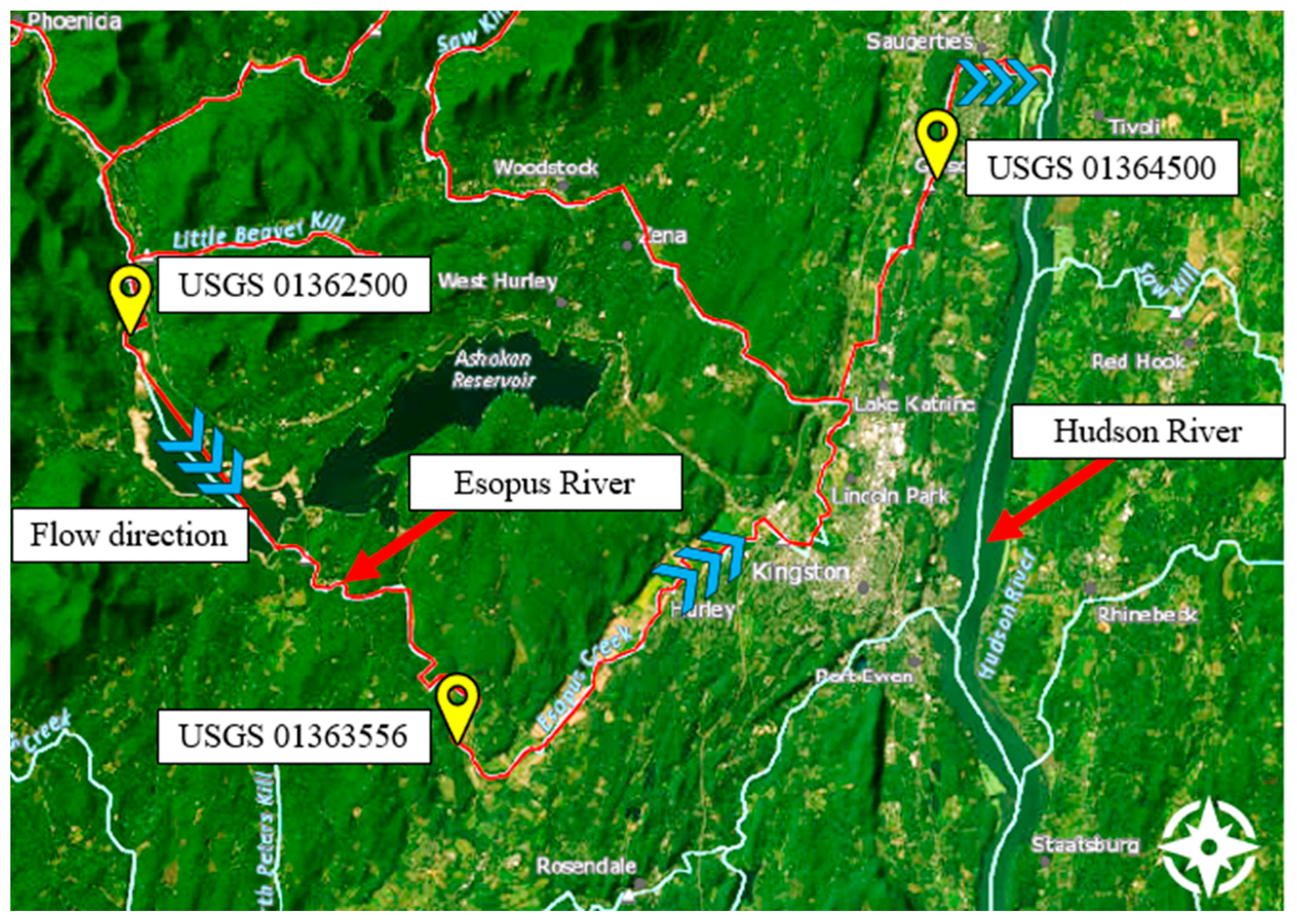
Figure 3.
Input variables distribution, USGS 01362500 (a), USGS 01363556 (b), and USGS 01364500 (c) using histogram and density plot.
Figure 3.
Input variables distribution, USGS 01362500 (a), USGS 01363556 (b), and USGS 01364500 (c) using histogram and density plot.
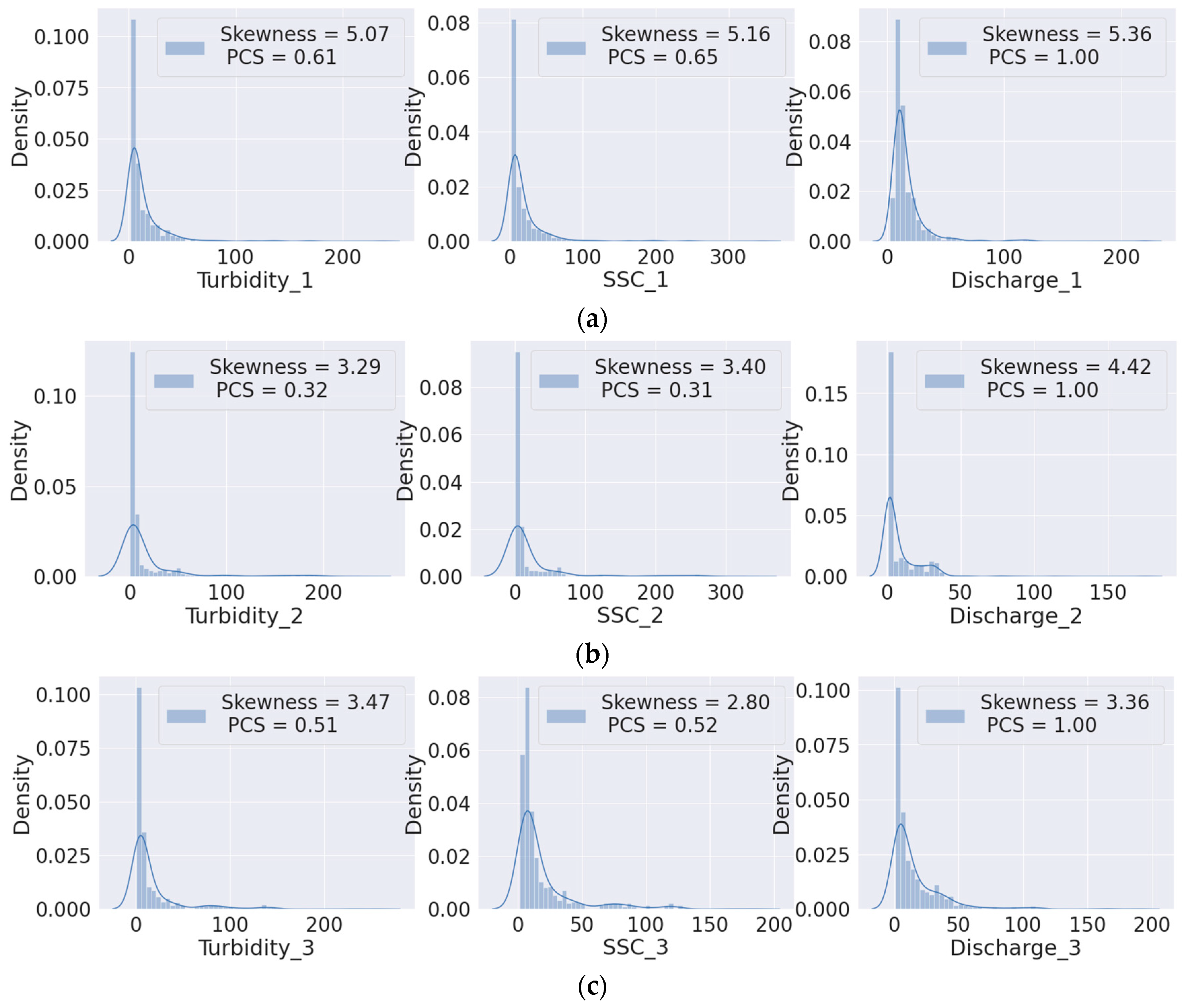
Figure 4.
Bivariate correlation coefficients among the input variables of three USGS gauges represented by the correlation heatmap.
Figure 4.
Bivariate correlation coefficients among the input variables of three USGS gauges represented by the correlation heatmap.
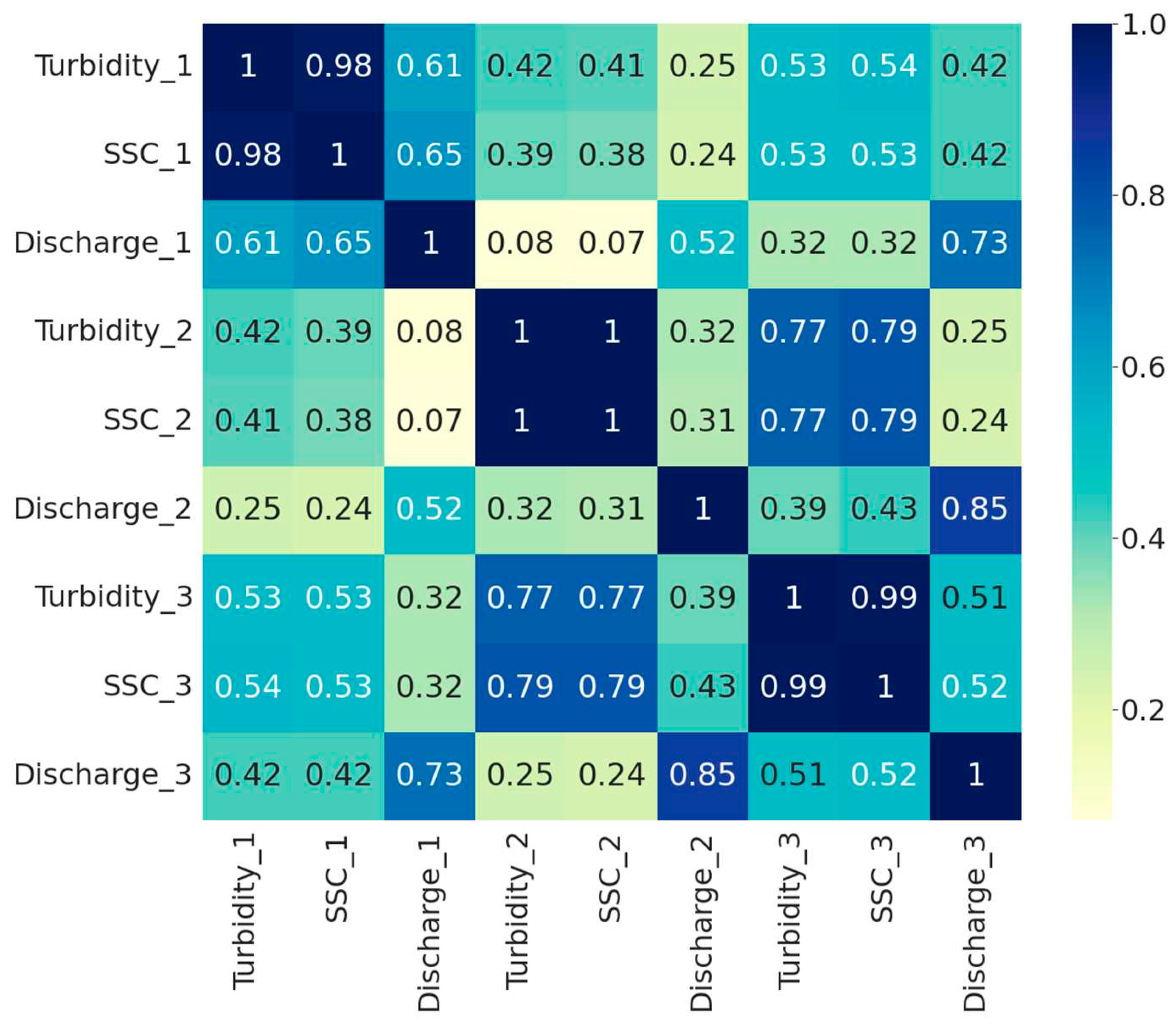
Figure 6.
LSTM results; Scenario 1: prediction SSC_3 by the most relevant feature (a), Scenario 1: prediction Discharge_3 by the most relevant feature (b), Scenario 2: prediction SSC_3 by three most relevant feature (c), Scenario 2: prediction Discharge _3 by three most relevant feature (d), Scenario 3: prediction SSC_3 by four most relevant feature (e), Scenario 3: prediction Discharge _3 by four most relevant feature (f).
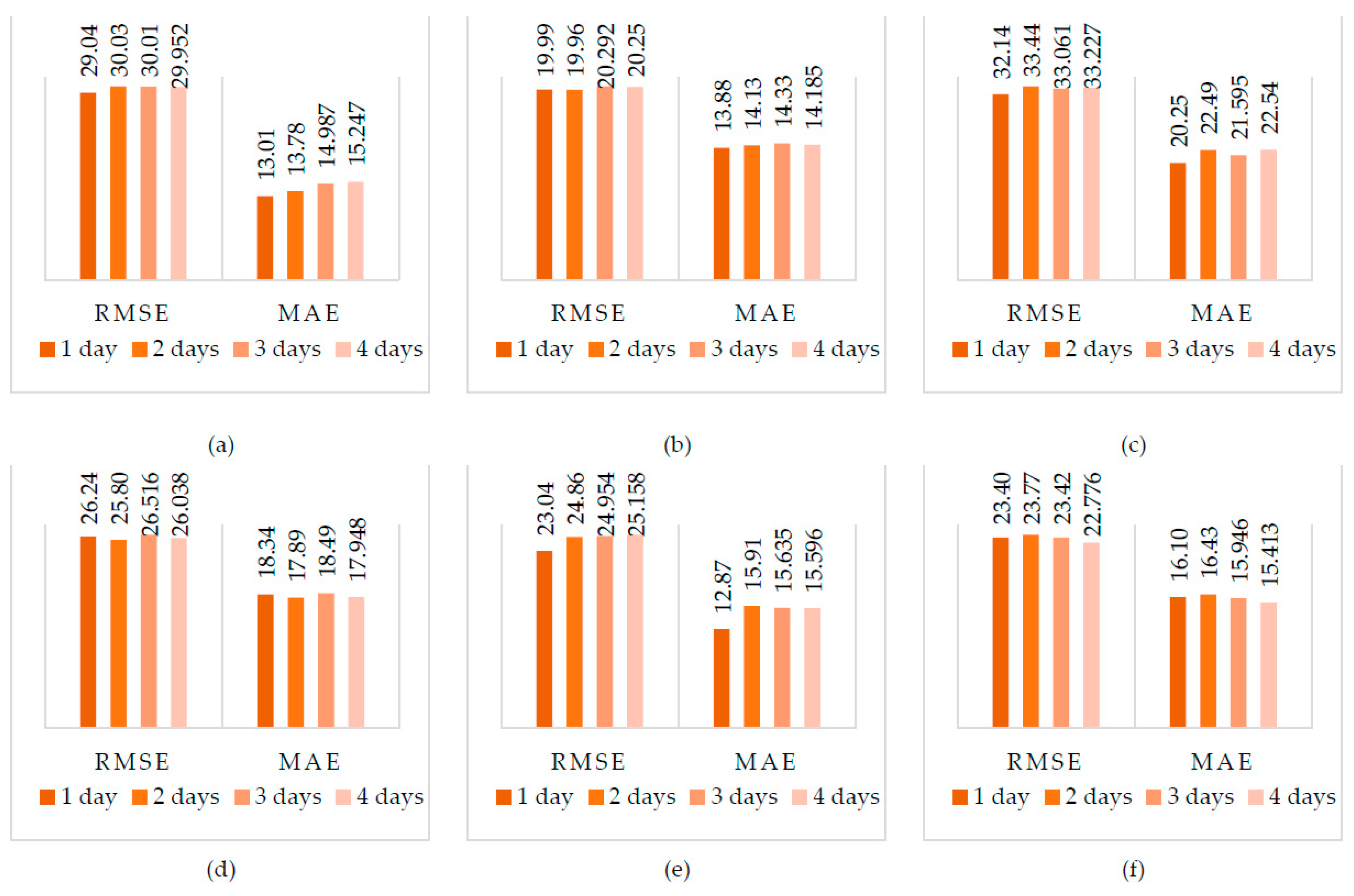
Table 3.
Descriptive Statistics of the studied variables.
| Count | Mean | Std | Min | 25% | 50% | 75% | Max | |
|---|---|---|---|---|---|---|---|---|
| Discharge_1 | 580 | 16.94 | 17.29 | 2.79 | 9.26 | 11.83 | 18.36 | 219.74 |
| Discharge_2 | 581 | 9.08 | 14.69 | 0.72 | 1.38 | 2.16 | 11.86 | 174.43 |
| Discharge_3 | 581 | 16.41 | 21.79 | 1.55 | 3.65 | 8.01 | 21.15 | 187.46 |
| Turbidity_1 | 562 | 13.52 | 20.91 | 1.70 | 3.90 | 6.20 | 14.58 | 235.00 |
| Turbidity_2 | 575 | 18.47 | 38.53 | 0.60 | 1.90 | 3.70 | 9.85 | 237.00 |
| Turbidity_3 | 565 | 17.28 | 30.79 | 0.70 | 3.10 | 5.10 | 14.40 | 255.00 |
| SSC_1 | 579 | 18.36 | 30.64 | 2.00 | 4.80 | 7.80 | 19.50 | 345.00 |
| SSC_2 | 575 | 23.63 | 52.09 | 0.60 | 2.00 | 4.00 | 11.50 | 328.00 |
| SSC_3 | 565 | 19.20 | 26.12 | 1.60 | 5.60 | 8.40 | 19.20 | 183.00 |
Table 4.
Recursive Feature Elimination (RFE) results for the most relevant features to predict SSC downstream.
Table 4.
Recursive Feature Elimination (RFE) results for the most relevant features to predict SSC downstream.
| Selection among | Most relevant features |
|---|---|
| All features | ‘Turbidity_3’, ‘Turbidity_1’, ‘Discharge_3’, ‘SSC_1’ |
| Dropping turbidity’ values | |
| 4 top features | ‘SSC_2′, ‘Discharge_3’, ‘SSC_1’, and ‘Discharge_1’ |
| 3 top features | ‘SSC_2′, ‘Discharge_3’, and ‘Discharge_1’ |
| 2 top features | ‘SSC_2′, and ‘Discharge_3’ |
| 1 top feature | ‘SSC_2’ |
Disclaimer/Publisher’s Note: The statements, opinions and data contained in all publications are solely those of the individual author(s) and contributor(s) and not of MDPI and/or the editor(s). MDPI and/or the editor(s) disclaim responsibility for any injury to people or property resulting from any ideas, methods, instructions or products referred to in the content. |
© 2023 by the authors. Licensee MDPI, Basel, Switzerland. This article is an open access article distributed under the terms and conditions of the Creative Commons Attribution (CC BY) license (http://creativecommons.org/licenses/by/4.0/).
Copyright: This open access article is published under a Creative Commons CC BY 4.0 license, which permit the free download, distribution, and reuse, provided that the author and preprint are cited in any reuse.


