Submitted:
12 May 2023
Posted:
16 May 2023
You are already at the latest version
Abstract
The goal of the manuscript is to design a relatively best control structure for the noise suppression of a drone’s camera gimbal action. The gimbal’s movement can be simplified as a rest-to-rest reorientation system that can achieve the boundary result of a dynamic system. Six different control architectures are proposed and evaluated based on their ability to control the trajectory of the dynamic-system position and speed, their running time, and quadratic cost. The robustness of the control architecture to uncertainties in inertia and sensor noise is also analyzed. Monte Carlo figures are used to assess the performance of the six control systems. The conditions for applying different architectures are identified through this analysis. The analysis and experimental tests reveal the most suitable control of the drone’s camera gimbal rotation.
Keywords:
P+V controller
; Double integrator patching filter
; control law inversion patching filter
; RTOC control
; open loop control
; feedback control
; Monte Carlo model
1. Introduction
1.1. The introduction to the drone and its single-axis camera control
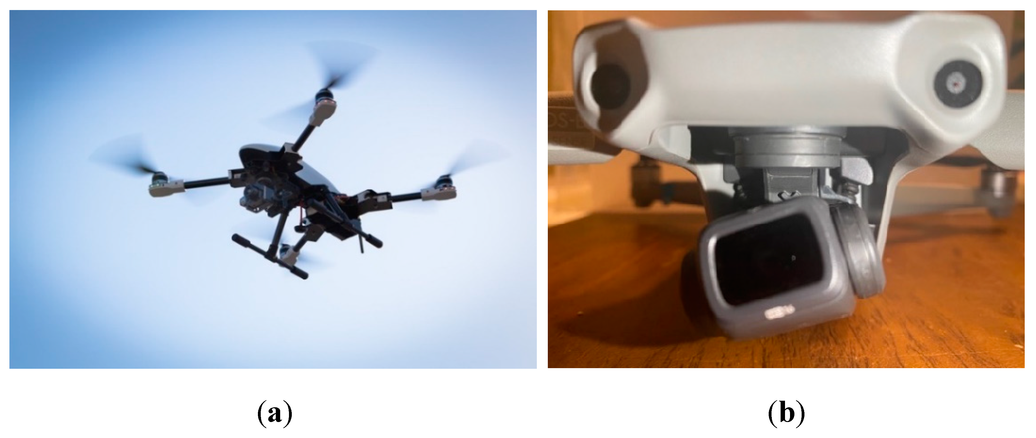
Drones, also known as unmanned aerial vehicles (UAVs), are a type of aircraft that can be controlled remotely without a pilot onboard. The history of drones began after the First World War when simple prototypes is used as weapons. [1] During the late twentieth century, an autonomous control system is added to aid operations. Currently equipped with advanced technologies such as global positioning systems (GPS), [2] cameras, and sensors [3], drones has the indigenous abilities for navigation, data collection, videography, or some specific mission objectives.
Figure 1.
(a) NASA uses drones for launch detection. image credit NASA [4] Images used in accordance with image use policy, “NASA content (images, videos, audio, etc.) are generally not copyrighted and may be used for educational or informational purposes without needing explicit permissions”. [5] (b) the detail of the one-gimbal drone’s camera.
The drone is becoming increasingly important in a wide range of industries, including agriculture construction [6,7], journalism, [8] and filmmaking [9], among others; and drones of various sizes and shapes have been designed for a wide range of applications proving drones to be a growingly important technological advancement and an increasingly vital tool for modern society.
Cameras are a very common payload for drones, as they enable users to capture images and videos from a unique perspective which would be different from that obtained by traditional cameras on the ground. As the basis of robot perception, cameras serve as eyes for aerial photography and videography, surveying and mapping, and inspection and monitoring of infrastructure and facilities. [10] Thus, cameras are a crucial component of modern drones, and their performance will also directly impact the performance of the drone.
Error caused by camera mounting devices is considered one of the main factors affecting camera performance. Sources of noise affect the performance of the camera leading to pointing deviation and vibrations. Various camera mounting devices are available, as described by Carmona [11], who has designed a complex platform-style mechanical structure that can stabilize the camera and absorb vibrations. Unfortunately, complex mechanical structures can be relatively cumbersome for drones that aim to be small and affordable. Danh [12] described a dual-axis gimbal that stabilizes the camera, but the design still requires an excellent control structure to support system operations. One widely-accepted solution is to use a single-axis gimbal and electrical control structure to mount the camera, as explained in Gasparovic’s article [13] where the advantages of the gimbal are clearly outlined.
1.2. Introduction to gimbal control research
1.2.1. Challenges in the manipulation of the gimbal rotation
The motion model of the gimbal is not complex and may be expressed as Euler’s moment equation to model rotation. Accurately rotating the gimbal to a specific angle is a task whose challenge resides in the required pointing accuracy. Within a limited time, frame, the gimbal is required to start from a stationary state, rotate to a specific angle, and maintain a stationary state with zero speed or acceleration at the end. Such rest-to-rest motion of a rigid body system is the focus of this manuscript. With the use of electronic control structures, precise control is theoretically possible, but necessitates wise selection of a suitable control amidst sensor(s) noise and parameter variations with time.
1.2.2. Similar former efforts
At the fundamental level, Kim and Byum [14] explain the basic proportional, integral, derivative (PID) control method applied to the stabilization control of drone gimbals, as well as the tuning process. Similar to PID control [15], other control methods such as Proportional plus velocity (P+V) control and optimum control can also be applied to drone camera gimbals seeking to maintaining higher accuracy [16]. Lassak [17] explains the importance of a pre-filter for patching the control, which helps the structure achieve control objectives better and faster. Real-time control [18] is also crucial for a motion mechanism like a drone, and Aguilar [19] presented a real-time image control method for drones. The approach is also applicable to gimbal control. [20,21] For simulating real environments, the noise in the sensors is a significant factor and the Monte Carlo model is particularly prominent in analyzing the impacts of noise on pointing accuracy. [22] The application of Monte Carlo by Binder [23] is a good example of such data analysis. Lastly, analysis of multiple controls [24] provides a comparative analysis of different optimal-control structures. Each disparate control structure has advantages and disadvantages in different situations. [25]
1.3. The rest-to-rest model of the drone’s gimbal and six controls
The movement of a drone’s camera gimbal is mathematically modeled as rest-to-rest rotation of a rigid body system, which means that its velocities and acceleration at the beginning and end points are zero (quiescent conditions) over a specified, limited time. The rest-to-rest rigid-body system adheres to classical Newtonian translation mechanics and rotation in accordance with Euler’s moment equations [26] represented as a double integrator in equation (1) when motion is expressed in coordinates of an inertial reference frame. The rotation equation of the reorientation system is the focus of control and optimization.

Table 1.
Proximal variable definitions.
| Valuables | Definitions | Valuables | Definitions |
|---|---|---|---|
| Angle | the quadratic cost functional | ||
| Angular velocity | The dynamic cost function | ||
| Rotational acceleration | The dynamic constraint | ||
| The inertia of moment | System torque | ||
| The initial time | The final time | ||
| u | Control function of time |
Such tables are distributed throughout the manuscript to increase the ease of reading, while a combined, master table of definitions is included in the appendices.
The boundary condition for the rest-to-rest maneuver is characterized by starting from a stationary position and ending with a new orientation with zero velocity. The expected duration of the maneuver is scaled or normalized to unity. The boundary condition in this problem is expressed in equation (2). In addition, the performance of the controller is also evaluated using the quadratic cost displayed in equation (3). The control architecture tuned the relevant parameters and appropriate values were selected to minimize the quadratic cost.
There are six control architectures compared are:
- Proportional plus velocity feedback control.
- Real-time optimal control. [29]
- Proportional plus velocity feedback with a double-integrator patching filter. [30]
- Gain-(re)tuned P+V controller with a double-integrator patching.
- Proportional plus velocity controller with a control law inversion patching filter.
Table 2.
Acronym definitions.
| Topic | Definitions |
|---|---|
| RTOC | Real-Time optimal control |
| P+V | Proportional plus velocity control |
| HzMAT | Hamiltonian Minimization, Adjoint equations, Terminal transversality of the endpoint Lagrangian |
| Kp and Kv | Proportional and velocity gains for P+V control |
Such tables are distributed throughout the manuscript to increase the ease of reading, while a combined, master table of definitions is included in the appendices.
The main controller architectures compared in this manuscript are the proportional plus velocity (P+V) controller with and without patching filters; double-integrator quadratic cost control (DQC) as both open-loop optimal control and real-time optimal control (RTOC) with feedback. [31]
The proportional plus velocity (P+V) feedback controller is similar to the well-known proportional, integral, derivative (PID) controller, and to proportional, derivative (PD) control. Proportional plus velocity control contains an amplifier to adjust the state variables towards the target and does not necessitate an integrator to stabilize oscillations. The controller is simple to operate and easy to build. Compared to the open loop controller, the proportional plus velocity controller has better robustness to uncertainty. However, the controller has two parameters introducing tasks to tune effectively. Accuracy and precision are sought without inclusion of analytic minimization of quadratic costs.
The optimal-control algorithm is based on Pontryagin’s minimize principle, which converts the optimal control problem into a multipoint boundary value problem (BVP) where adjoint equations are used to incorporated constraints [32,33,34] as described in equations (4) – (9). The Hamiltonian minimization condition is expressed in equation (5). The adjoint equations are listed in equation (6). The terminal transversality condition of the endpoint Lagrangian is displayed in equation (7) and proves useful to provide additional boundary values aiding analytic solvability. The Hamiltonian final value condition does similarly.
The advantage of using the optimal-control algorithm resides in the influence of the quadratic cost and running time mandates. The final control result minimizes the cost while strictly enforcing the running time. Augmenting optimal-control results in the open-loop controller with feedback leads to a real-time system.
Table 3.
Table of proximal variable definitions.
| Variables | Definitions | Valuables | Definitions |
|---|---|---|---|
| Hamiltonian | Dynamic cost function | ||
| , | Lagrange multipliers | Dynamic constraint | |
| Lagrange multiplier for | Lagrange multiplier derivative for | ||
| x | System states | Control (a function of time) | |
| Total end-point cost functional | Static cost function | ||
| Static constraint function | Final time |
Such tables are distributed throughout the manuscript to increase the ease of reading, while a combined, master table of definitions is included in the appendices.
2. Materials and Methods
2.1. The HzMAT optimal to the rest-to-rest orientation system
Based on Equation (3), the quadratic cost function is considered, and identify that the F in Equation (4) represents a dynamic cost in the system which is generated by the quadratic cost. Therefore, the dynamics or running cost presents the link relation between the quadratic cost and dynamic system constraint. Equation (10) is the quadratic cost function:
The f in the Hamiltonian condition is a dynamic constraint in the system. External control in the dynamics depends on the costate, state, and time. The costate represents the sensitivity of the system to perturbations and the states represent the current physical state of the system. Additionally, time is also a critical factor in external control since the time determines the duration of the control action and influences the overall performance of the system. Equation (11) displays the relationship between the dynamics and these factors.
Equation (11) provides insight into the relationship between the dynamic’s constraint and states. Equation (12) shows that the detail of dynamic constraint, represented by f in the Hamiltonian, influences the evolution of the state variables over time. The dynamic constraint is simplified by expressing the constraints as a set of equations that maintain the simplest structure, consisting of a first derivative and a derivative-free function.
For each state variable in the system, there is a corresponding costate variable, which represents the sensitivity of the system’s performance to perturbations in that state variable. Therefore, the Hamiltonian condition function is a combination of dynamic cost and dynamic constraints by Lagrangian, which include both the state and costate variables.
Based on Equation (5), the result of the partial derivative of the Hamiltonian condition functions with respect to the control value is calculated.
Therefore, referring to Equation (6), the adjoint equations in this condition are available. Equations (15) and (16) obtained by taking the partial derivative of the and using the Hamiltonian function are:
Table 4.
Table of proximal variable definitions.
| Variable | Definition |
|---|---|
| The torque from the controller | |
| The Lagrangian about | |
| The Lagrangian about | |
| The derivative about the lagrangian | |
| The derivative about the lagrangian |
Such tables are distributed throughout the manuscript to increase the ease of reading, while a combined, master table of definitions is included in the appendices.
Equations (15) and (16) establish the relationship between the Lagrangian and constant through integral operation, while equations (17) and (18) demonstrate the obtained result:
where a and b are both constant.
By combining Equations (17) and (18), a straightforward relationship between control and time can be derived in Equation (20).
Integrate these equations and obtain the optimal control for both velocity v and angle .
where a, b, c, and d are unknown constants.
Equations may contain unknown constants, therefore constructing a solvable equation needs to base on time and control. The solution to the equation requires the specification of boundary conditions. After satisfying these conditions, a time-optimal control under the given conditions is available.
Due to the boundary condition in Equation (2), the control function with respect to time from Equation (19) to (21) is displayed in Equation (23), (24) and (25):
Table 5.
Table of proximal variable definitions.
| Variable | Definition |
|---|---|
| t | Time (dimensionless) |
| a, b, c | Constants of integration |
Such tables are distributed throughout the manuscript to increase the ease of reading, while a combined, master table of definitions is included in the appendices.
2.2. The introduction of six control architectures
2.2.1. Open loop controller with the result of the HzMAT optimal analysis
By utilizing the optimal analysis result from the HzMAT with equation (22) as input, the ideal output for both theta and angular velocity can be derived through double integrator translation control. The control architecture is depicted in Figure 3:
Figure 2.
Open-loop controller structure.
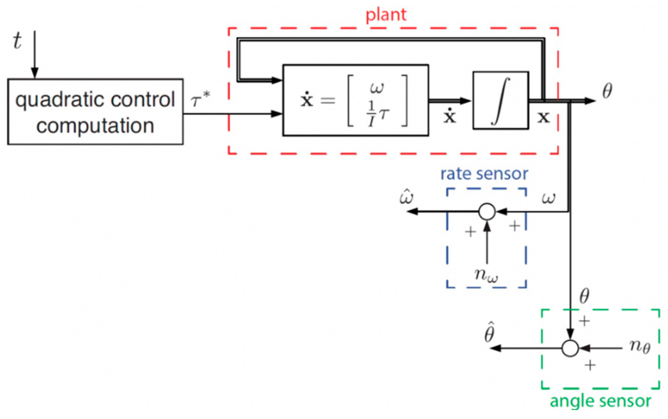
Figure 3.
P+V feedback controller structure.
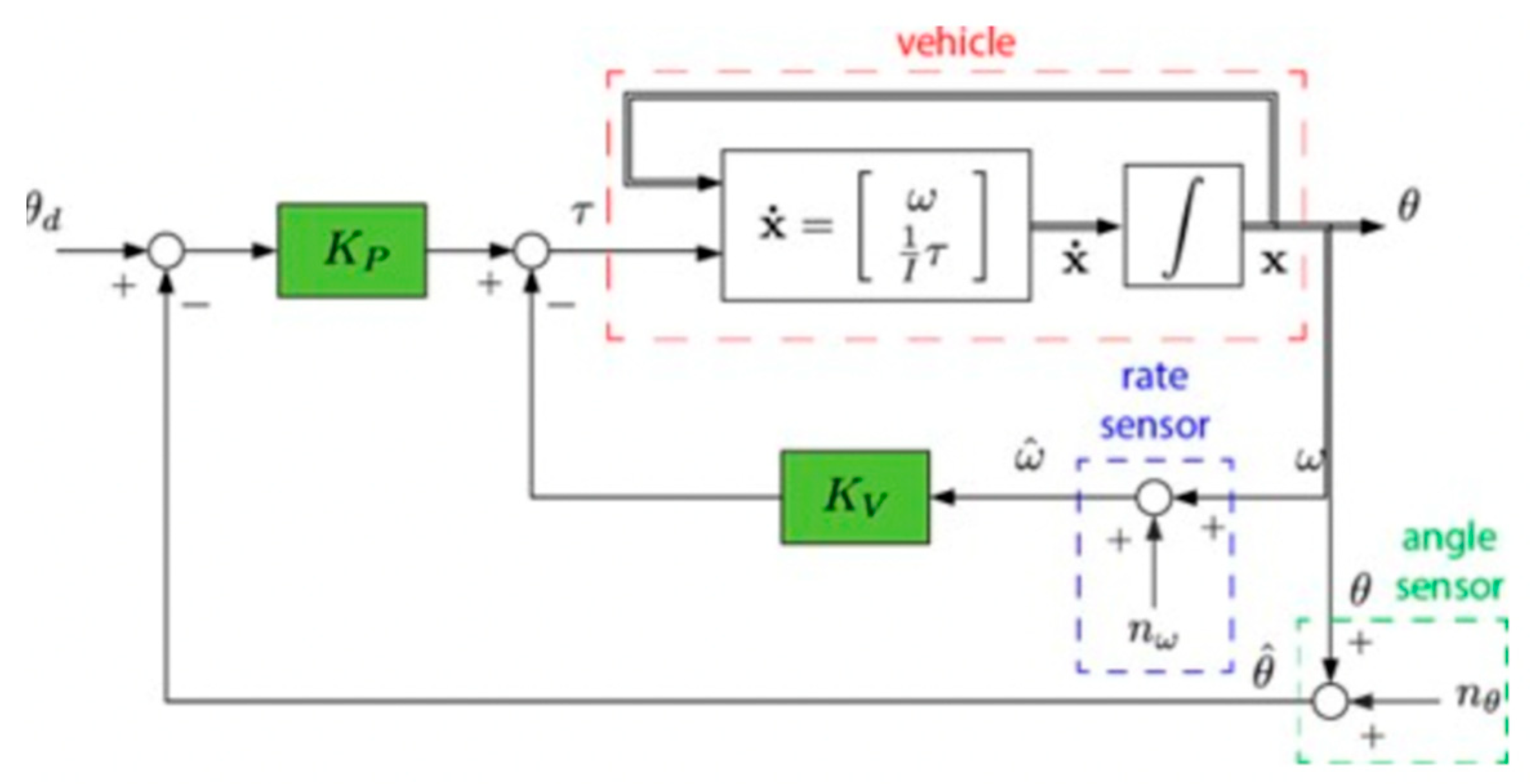
2.2.2. P+V feedback controller
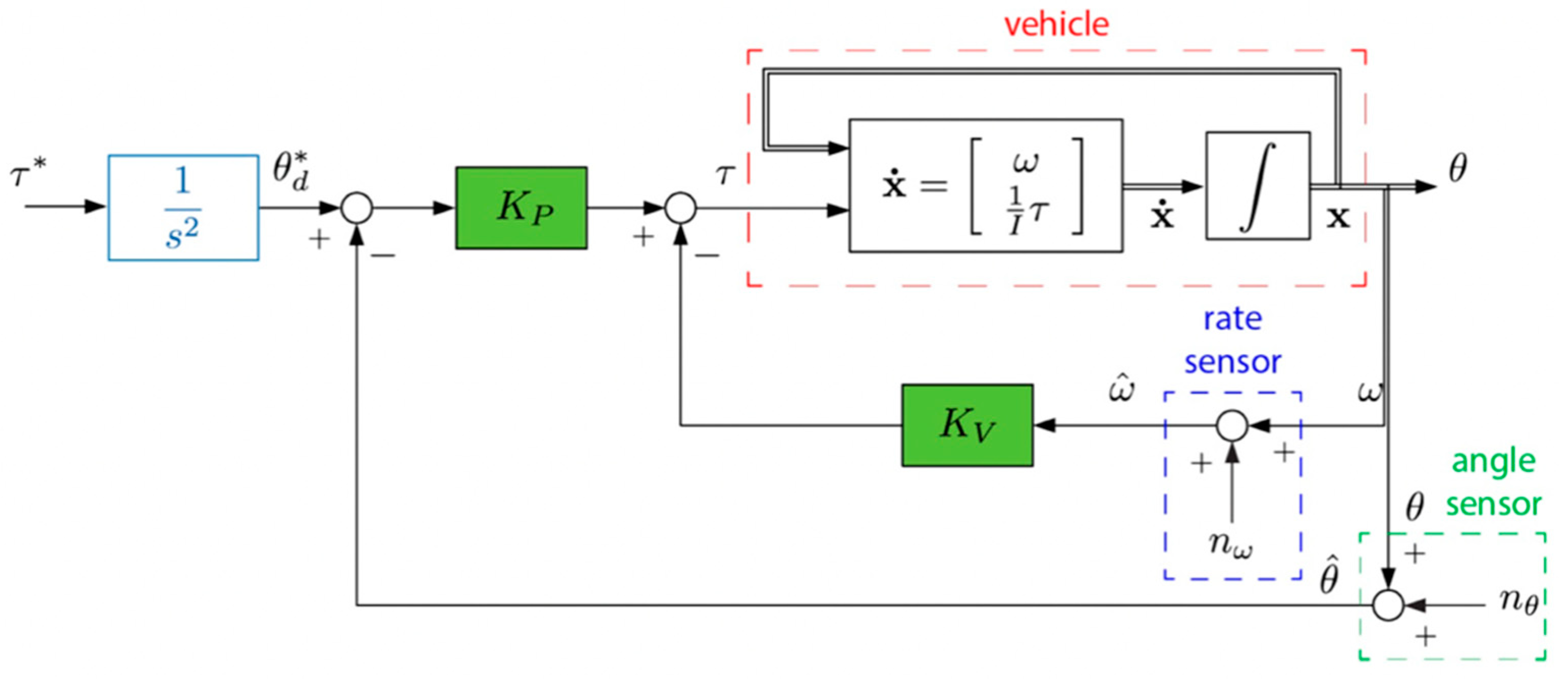
Due to the feedback system, an ideal target (shown in Figure 4) is set and the error between the target and the output theta can be calculated. The error is then multiplied by and added to Kv times the output speed, forming the system input. After passing through the double integrator, the system provides output values for both theta and speed, which are then fed back into the input, completing the feedback loop.
Figure 4.
RTOC controller structure.
The values of Kv and Kp used in this system are tuned based on the analysis of oscillation. the system’s steady state can be set as and . Where is the angular speed obtained from oscillation analysis, and is a parameter related to the system’s running time.
Table 6.
Table of proximal variable definitions for Figure 3 and 4.
| Variable | Definition |
|---|---|
| The desired angle | |
| The position output | |
| Kv | A proportional value for P+V control |
| Kp | A proportional value for P+V control |
| x | System states |
| The derivative of states | |
| The velocity output | |
| The actual velocity (the velocity output with the noise) | |
| The actual angle (the position output with the noise) | |
| The noise from the position sensor | |
| The noise from the velocity sensor |
Such tables are distributed throughout the manuscript to increase the ease of reading, while a combined, master table of definitions is included in the appendices.
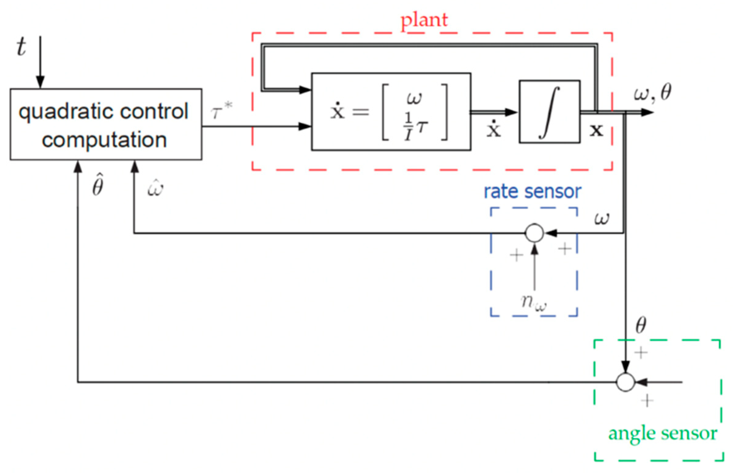
2.2.3. Real-time optimal controller (RTOC)
RTOC is a real-time controller (shown in Figure 5) that utilizes the HzMAT optimization with different boundary conditions. The HzMAT analysis can provide reference equations like equations (20), (21), and (22). Various final boundary conditions can help to solve the values of a, b, c, and d. These values will be utilized to determine the control u and subsequently calculate the output position and speed of the system. But in this manuscript, time, position, and velocity limitations keep the same for easy comparison.
Figure 5.
P+V feedback controller with double integrator patching filter.
2.2.4. P+V feedback control with double-integrator patching filter.
In the P+V feedback controller, a patching filter is introduced to optimize the basic target and enhance the system’s input to approach the ideal target. In the patching filter, there is a simple double integrator (shown in Figure 6) that closely represents the dynamics of the open-loop plant. The Kp and Kv parameters remain unchanged.
Figure 6.
P+V controller with Control law inversion patching filter structure.
| Variable | Definition |
|---|---|
| s | Complex variable for Laplace Transform |
| The desired transformed angle | |
| The desired torque input | |
| The velocity output | |
| The position output | |
| The actual velocity (the velocity output with the noise) | |
| The actual angle (the position output with the noise) | |
| The noise from the position sensor | |
| The noise from the velocity sensor |
Such tables are distributed throughout the manuscript to increase the ease of reading, while a combined, master table of definitions is included in the appendices.
2.2.5. Gain-tuning P+V controller with double-integrator patching.
This control architecture still utilizes the P+V feedback control structure, complemented by a double integrator patching filter. However, the Kp and Kv parameters have been updated with brand-new values that are tested to improve the system’s ability to approach the ideal target. After careful selection and tuning, the Kp and Kv are set to 400 and 3, respectively.
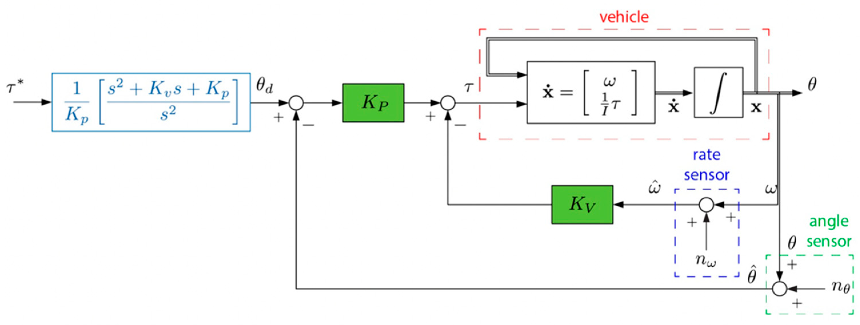
2.2.6. P+V controller with Control law inversion patching filter.
This controller architecture is like the previous structure, with the primary difference being the use of a control law inversion patching filter. To achieve the HzMAT optimal control with the P+V controller, the input must be designed to be close to the final output.
Table 8.
variables definitions.
| Variables | Definitions | Variables | Definitions |
|---|---|---|---|
| The desired angle | The input of the control structure (angle) | ||
| The actual angle | The output of the control structure (control) | ||
| The desired control | Kv | A proportional value for P+V control | |
| u | The actual control | Kp | A proportional value for P+V control |
Such tables are distributed throughout the manuscript to increase the ease of reading, while a combined, master table of definitions is included in the appendices.
As a reminder, the closed-loop control law is displayed in the equation (25):
Also, equation (25) can be written as equation (26) and (27). Equation (27) represents the ideal outcome of equation (26).
For the double integrator plant, equation (28) is the same as equation (27):
Equation (28) may be written in the s-domain based on Laplace Transform as
Therefore, an alternative patching filter is shown in the equation (30):
The control structure is displayed in Figure 7:
Figure 7.
MATLAB® integration solver iteration with time on the abscissa and position and velocity on the ordinant. (a) the trajectory under the ode1 and step 0.01. (b) the trajectory under the ode4 and step 0.01. (c) the trajectory under the ode4 and step 0.0001.
Figure 7.
MATLAB® integration solver iteration with time on the abscissa and position and velocity on the ordinant. (a) the trajectory under the ode1 and step 0.01. (b) the trajectory under the ode4 and step 0.01. (c) the trajectory under the ode4 and step 0.0001.
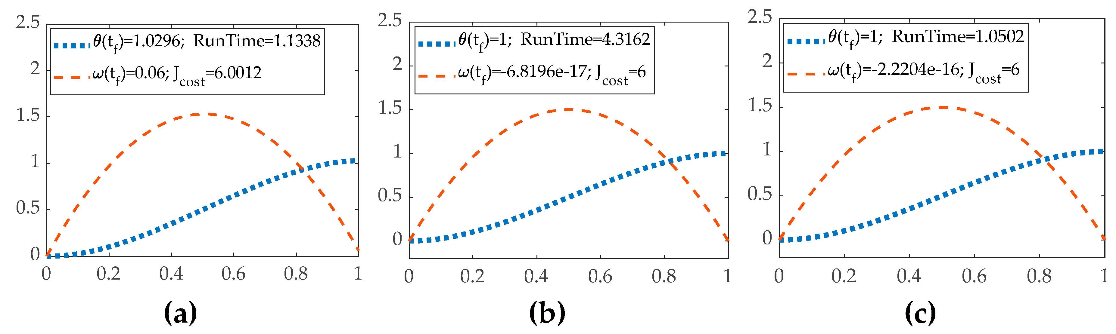
Table 9.
Table of proximal variable definitions for Figure 7.
| Variable | Definition |
|---|---|
| s | Complex variable for Laplace Transform |
| Kv | A proportional value for P+V control |
| Kp | A proportional value for P+V control |
| The actual velocity (the velocity output with the noise) | |
| The actual angle (the position output with the noise) | |
| The noise from the position sensor | |
| The noise from the velocity sensor |
Such tables are distributed throughout the manuscript to increase the ease of reading, while a combined, master table of definitions is included in the appendices.
2.3. The MATLAB® solver selection
In the Simulink system, the solver plays a crucial role in determining the trajectory of the position and speed variables. Thereby the solver affects the accuracy and precision of the results. Therefore, selecting the appropriate solver and step size carefully for the analysis of the controllers’ performance is essential.
For the purposes of this manuscript, using an open-loop controller to evaluate the solver is convenient. When ode1 with a step size of 0.01 is tested, the resulting trajectory appears in Figure 8 (a). To obtain more accurate results, using a different solver as a comparison is significant, such as ode4 with a step size of 0.01 whose trajectory is displayed in Figure 8 (b). To further improve the accuracy and precision of the results, reducing the step size to 0.0001 is also an option, The objective trajectory with a step size of 0.0001 is shown in Figure 8 (c).
Figure 8.
MATLAB® simulations with no noise with time on the abscissa and position and velocity on the ordinant. (a) The trajectory from the open loop. (b) The trajectory from the P+V controller. (c) The trajectory from the RTOC.
Figure 8.
MATLAB® simulations with no noise with time on the abscissa and position and velocity on the ordinant. (a) The trajectory from the open loop. (b) The trajectory from the P+V controller. (c) The trajectory from the RTOC.
The conclusion based on the trajectory of ode1 with a step size of 0.01 is obvious that the final angular speed fails to satisfy the rest-to-rest condition. As a result, ode1 may not be the optimal choice for our analysis. After switching to the ode4 solver, the final boundary condition appears to be better satisfied in Figure 8 (b). Switching to the ode4 solver with a step size of 0.0001 did not significantly improve the final boundary condition. However, the running time increased significantly.
Table 10.
The performances of the open-loop system with different solvers and step length.
| Solver and step length | End position | End velocity | Computational runtime | Quadratic cost (vehicle fuel usage) |
|---|---|---|---|---|
| Ode1 solver with 0.01 step length | 1.0296 | 1.1338 | 6.0012 | |
| Ode4 solver with 0.01 step length | 1 | 1.0502 | 6 | |
| Ode4 solver with 0.0001 step length | 1 | 4.3162 | 6 |
Such tables are distributed throughout the manuscript to increase the ease of reading, while a combined, master table of definitions is included in the appendices.
To find a compromise between accuracy and efficiency, using the ode4 solve with a step size of 0.01 is an ideal option for the simulation. This should provide reasonably accurate results while also maintaining a manageable running time.
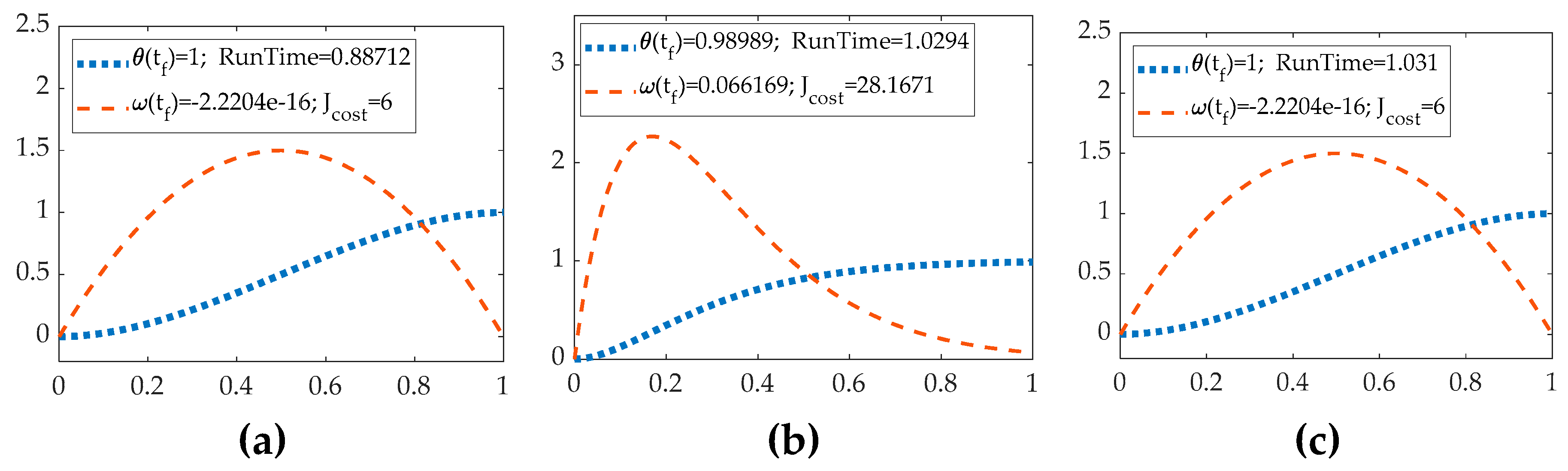
3. Trajectory of the result from six architectures without any uncertainty
Once the various control structures in Simulink are implemented, the resulting trajectories can be examined. Figure 9 (a), (b) and (c) show the trajectories obtained from each control system.
Figure 9.
MATLAB® simulations with no noise with time on the abscissa and position and velocity on the ordinant. (a) The trajectory from the P+V controller with double-integrator patching filter (b) The trajectory from the tuning parameter P+V controller with double integrator filter. (c) The trajectory from the P+V controller with law inversion filter.
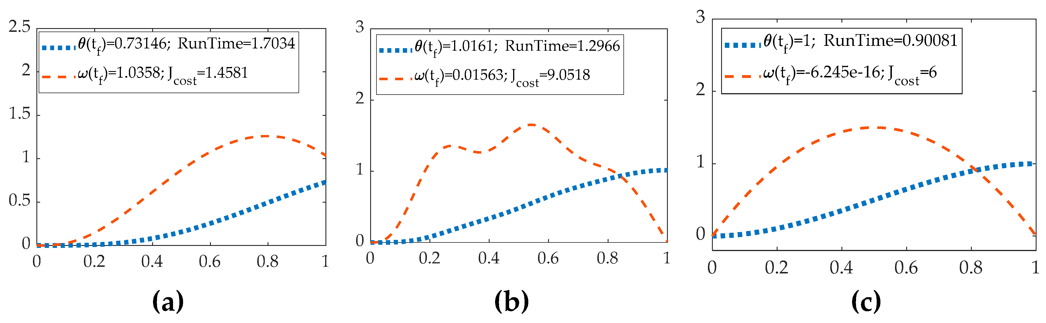
Table 11.
The performances of six control architectures without parameter variations.
| Vehicle control method | End position | End velocity | Computational runtime | Quadratic cost (vehicle fuel usage) |
|---|---|---|---|---|
| Open-loop optimal control, ideal case | 1 | 4.0003 | 6 | |
| Classical proportional + velocity feedback | 0.98989 | 3.4494 | 28.1671 | |
| Real-time optimal control | 1 | 3.8961 | 6 | |
| P+V control with double-integrator filter | 0.7315 | 1.0358 | 3.4832 | 1.4581 |
| Tuned-parameter P+V control with filter | 1.0161 | 0.015624 | 3.4747 | 9.0519 |
| P+V control with law inversion filter | 1 | 3.9615 | 6 |
Such tables are distributed throughout the manuscript to increase the ease of reading, while a combined, master table of definitions is included in the appendices.
Once the trajectories from different control structures are generated, the conclusion is obvious. Firstly, the HzMAT optimal controller provides significantly better precision and accuracy than the P+V controller. However, the HzMAT controller may cause a slight overshoot in the controlling, whether it is the open-loop controller or RTOC , as evidenced by the negative final boundary value of velocity. Secondly, by comparing the three figures of the P+V controller, the P+V controller with better tuning parameters of Kp and Kv and a suitable patching filter can provide accurate enough results. Thirdly, surprisingly, the open-loop controller achieved accuracy beyond our expectations, possibly due to the HzMAT optimal-control algorithm. It is worth noting that the ideal quadratic cost is 6, and the two types of HzMAT controllers performed better in terms of cost optimization, while the P+V controller incurred higher costs, even though they produced very similar trajectories. Finally, regarding running time, all P+V controller architectures had a shorter running time than the two types of HzMAT controllers.
4. Analysis of six control architectures with some uncertainties
After the uncertainties in inertia and sensor noises from the position and velocity sensors are added into the system, the trajectory demonstrates the distinct characteristics and robustness of different control architectures.
Figure 10.
MATLAB® simulations with noise with time on the abscissa and position and velocity on the ordinant. (a) The trajectory from the open loop with noise. (b) The trajectory from the P+V controller with noise. (c) The trajectory of RTOC with noise.
Figure 10.
MATLAB® simulations with noise with time on the abscissa and position and velocity on the ordinant. (a) The trajectory from the open loop with noise. (b) The trajectory from the P+V controller with noise. (c) The trajectory of RTOC with noise.
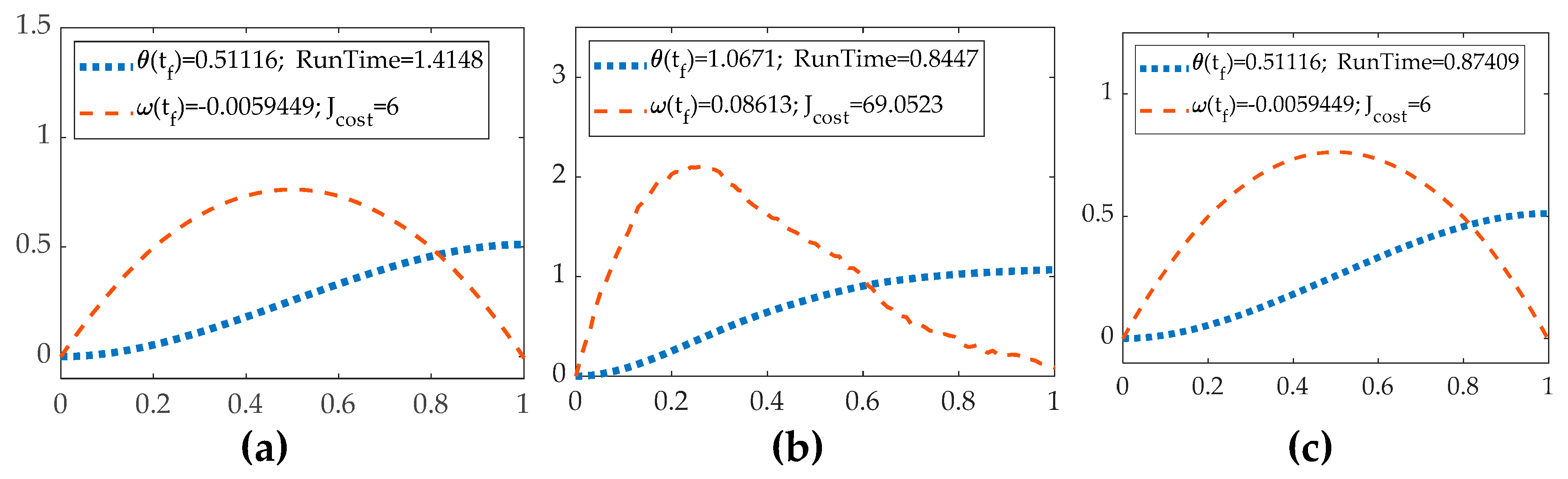
Figure 11.
MATLAB® simulations with noise with time on the abscissa and position and velocity on the ordinant. (a) The trajectory from the P+V controller with double-integrator patching filter with noise. (b) The trajectory from the tuning parameter P+V controller with double integrator filter with noise. (c) The trajectory from the P+V controller with law inversion filter with noise.
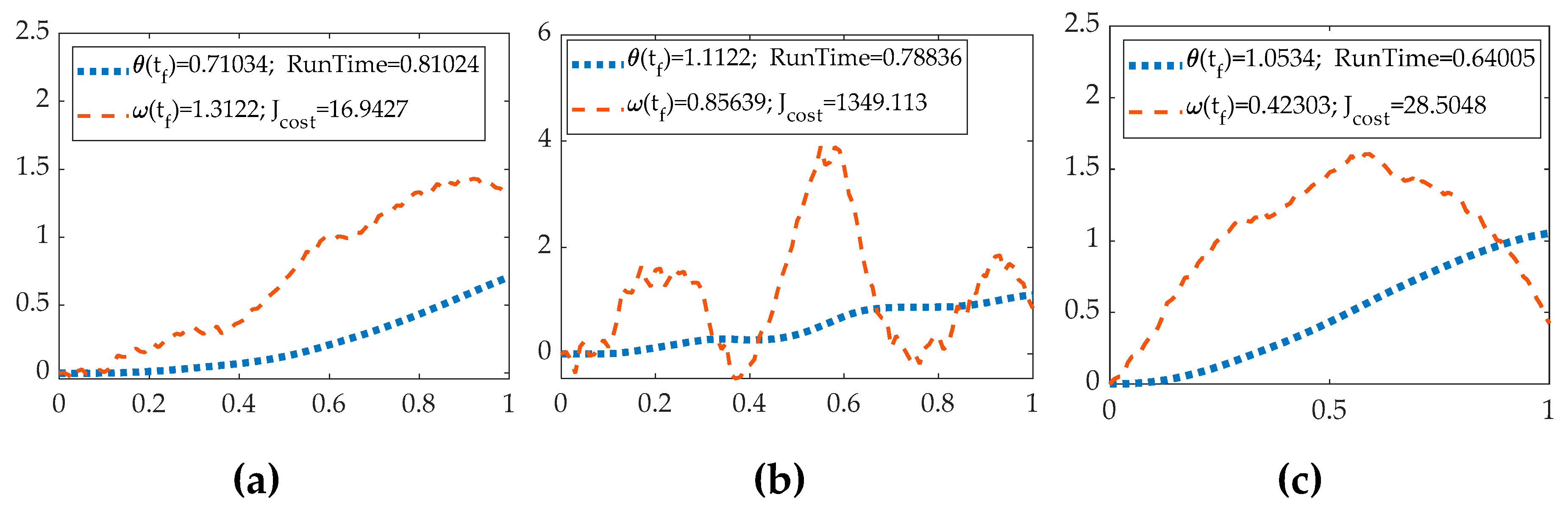
Table 12.
The performances of six control architectures with errors.
| Vehicle control method | End position | End velocity | Computational runtime | Quadratic cost (vehicle fuel usage) |
|---|---|---|---|---|
| Open-loop optimal control, ideal case | 0.511 | 4.1069 | 6 | |
| Classical proportional + velocity feedback | 1.0479 | 3.763 | 63.1212 | |
| Real-time optimal control | 0.51116 | -0.005945 | 4.1426 | 6 |
| P+V control with double-integrator filter | 1.0479 | -0.02946 | 3.6086 | 63.1212 |
| Tuned-parameter P+V control with filter | 0.96071 | 7.0317 | 3.617 | 20834.11 |
| P+V control with law inversion filter | 1.0479 | -0.02946 | 3.6246 | 63.1212 |
Such tables are distributed throughout the manuscript to increase the ease of reading, while a combined, master table of definitions is included in the appendices.
Surprisingly, despite the uncertainties, the open-loop controller’s trajectory remains like the condition without errors, which shows good robustness. It’s possible that only the uncertainty of inertia can affect the open-loop system, but its impact is limited. However, the theta result has a huge gap between the correct result set which means the open-loop controller is not suitable for the real environment. Also, uncertainties significantly affect the theta result of RTOC’s HzMAT controller. The P+V controllers’ trajectories show oscillation and are not as smooth as those from the HzMAT controller. Compared to the no-error system figures, a significant improvement in the performance of P+V controllers is that they keep high accuracy under the influence of errors. But the self-tuning patching filter amplified the errors’ impact, rendering the figure useless. The reason is poor tunning parameters, and this result presents the significance of tuning. In a conclusion, a well-set P+V controller in the error may yield a similar output to the HzMAT controller without errors. In terms of cost, the HzMAT control architectures are less expensive compared with the P+V controller.
5. Monte Carlo analysis
Monte Carlo analysis is a computational algorithm that uses random samples or parameters to generate a result in a target area. This Monte Carlo figure, also known as the distribution diagram, provides evidence of the impact of some specific parameters.
In this analysis, a large variety of random samples of error from the position and velocity sensors are selected and then the distribution diagrams for position and speed are generated to analyze the influence of two types of sensor noise.
Figure 12.
MATLAB® simulations with noise with the angle on the abscissa and the angular velocity on the ordinant. (a) Monte Carlo figure from the open loop (b) Monte Carlo figure from the single P+V controller (c) Monte Carlo figure from the RTOC.
Figure 12.
MATLAB® simulations with noise with the angle on the abscissa and the angular velocity on the ordinant. (a) Monte Carlo figure from the open loop (b) Monte Carlo figure from the single P+V controller (c) Monte Carlo figure from the RTOC.
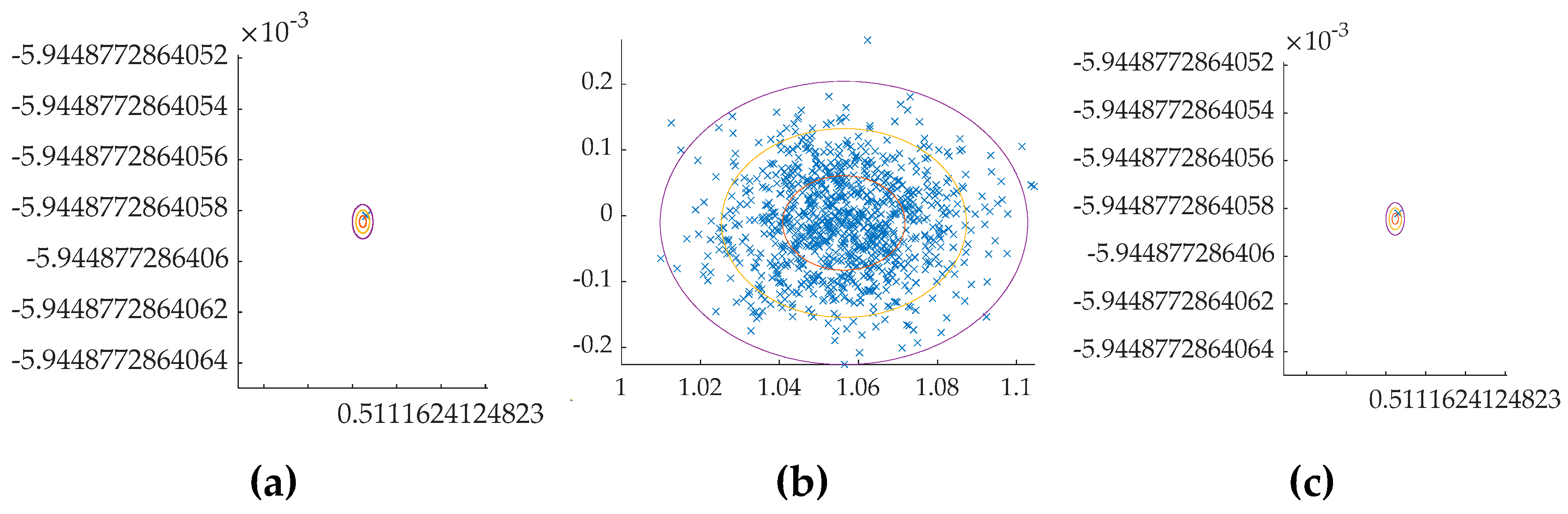
Figure 13.
MATLAB® simulations with noise with the angle on the abscissa and the angular velocity on the ordinant. (a) Monte Carlo figure from the P+V controller with double-integrator patching filter (b) Monte Carlo figure from the tuning parameter P+V controller with double integrator filter (c) Monte Carlo figure from the P+V controller with law inversion filter.
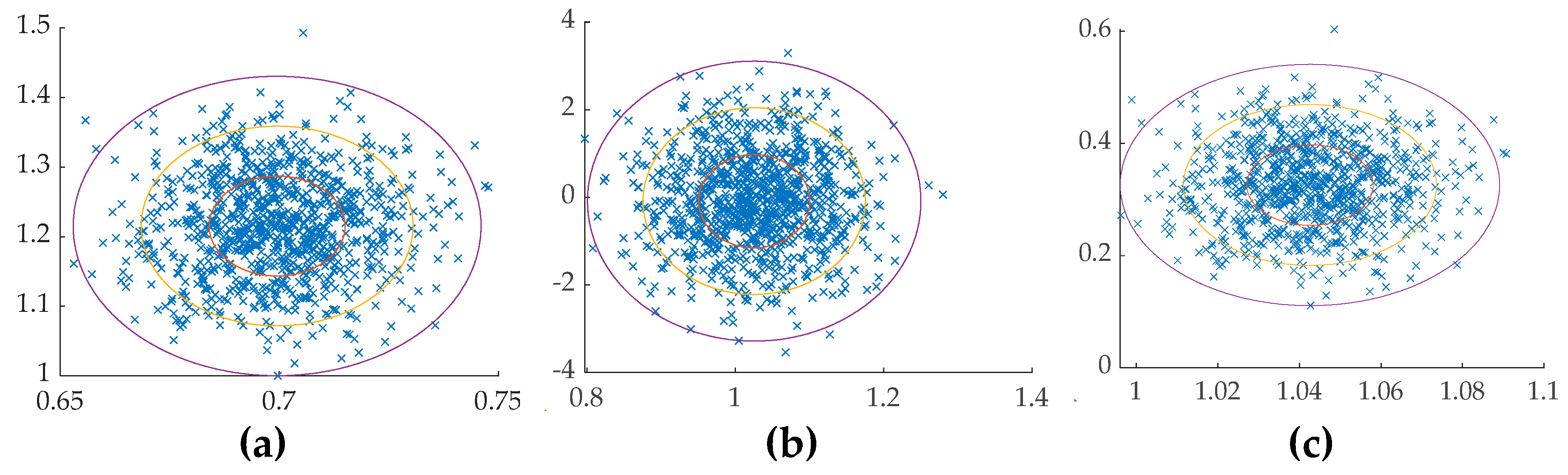
Table 13.
The performances of six control architectures with errors in Monte Carlo analysis.
| Vehicle control method | Mean final position | Final position deviation | Mean finalvelocity | Final velocitydeviation |
|---|---|---|---|---|
| Open-loop optimal control, ideal case | 0.5111624124 | |||
| Classical proportional + velocity feedback | 1.05552 | 0.01629 | -0.0103879 | 0.0503975 |
| Real-time optimal control | 0.51116241248 | -0.511162 | ||
| P+V control with double-integrator filter | 0.699979 | 0.01499 | 1.22195 | 0.0652 |
| Tuned-parameter P+V control with filter | 1.028792 | 0.069492 | -0.0148426 | 1.132874 |
| P+V control with law inversion filter | 1.04255 | 0.15541 | 0.328011 | 0.0735943 |
Such tables are distributed throughout the manuscript to increase the ease of reading, while a combined, master table of definitions is included in the appendices.
Open-loop controller is the least affected, as mentioned previously. all control architectures using P+V controllers are influenced by uncertainties. The Monte Carlo figures for the P+V controller with different filters show that Kp and Kv determine the degree of noise impact, and the patching filter is the one influenced by the uncertainty, despite its objective of closing the input to the final output. Surprisingly, the RTOC shows strong robustness. However, it’s undeniable that even the RTOC’s precision decreases due to uncertainties.
6. Discussions
The conclusion obtained from the findings from the model is that the HzMAT has great accuracy and precision in an ideal environment. However, in the real world with system noise, P+V, and HzMAT controllers have various disadvantages. For control architecture, the P+V controller with a law inversion filter has the best performance regardless of the noise level. Other P+V controllers seem good enough in a noisy environment.
If the dynamic system is fixed and has no obvious errors and requirements for real-time adjustment, then the open loop controller with the HzMAT value is the priority since it is not affected by sensor noise and is effective in controlling the system. However, open-loop control has no feedback system and is not suitable for use in a comprehensive dynamic system.
Gain–tuning patching filter and double integrator filter demonstrates that Kp/Kv and patching filter has a significant influence on the precision of P+V controller. Therefore, the idea of Law inversion is a good starting point for patching filters. Like the advantages and disadvantages of the HzMAT and P+V controller, RTOC is the priority when the sensor noise is small enough or cost optimization is necessary. However, when a simple computation algorithm or a less running time controller is needed in the real environment, the P+V controller with a law inversion filter is the priority.
Simple P+V controllers or P+V controllers with a double integrator can also be used. But the only advantage of these control architectures is their ease of operation. With appropriately tuned Kp and Kv, these controllers can also be applied in the real world.
Regarding patching filters, adjusting the input to be close to the final output is a good idea, and patching filters work like a feedforward control which influences the input value. Compared to a single P+V controller, the one with a double integrator patching filter or control law inversion patching filter has less robustness, although patching filters increase the precision.
When it comes to the control of the drone’s camera gimbal rotation, the P+V control with the law inversion patching is the priority in the complex real environment needing high precision. Also, RTOC is also suitable for general civilian products which don’t need high precision but need robustness. Other combinations of control structures like adding a feedforward patching for RTOC can be tested and added for the drone camera gimbal control in the future.
Author Contributions
Conceptualization, E.Z., and T.S.; methodology, E.Z. and T.S.; software, E.Z., and T.S.; validation, T.S.; formal analysis, E.Z., and T.S.; investigation, E.Z., and T.S.; resources, T.S.; data curation, E.Z., and T.S.; writing—original draft preparation, E.Z.; writing—review and editing, E.Z. and T.S.; visualization, T.S.; supervision, T.S.; project administration, T.S.; funding acquisition, T.S.
Funding
This research received no external funding. The APC was funded by the corresponding author.
Data Availability Statement
Data supporting reported results can be obtained by contacting the corresponding author.
Acknowledgments
Cornell University’s Jiren Liu provides a drone camera gimbal for research.
Conflicts of Interest
The authors declare no conflict of interest.
Appendix A
Figure A1.
MATLAB® simulation with noise in plant and state and rate sensors.
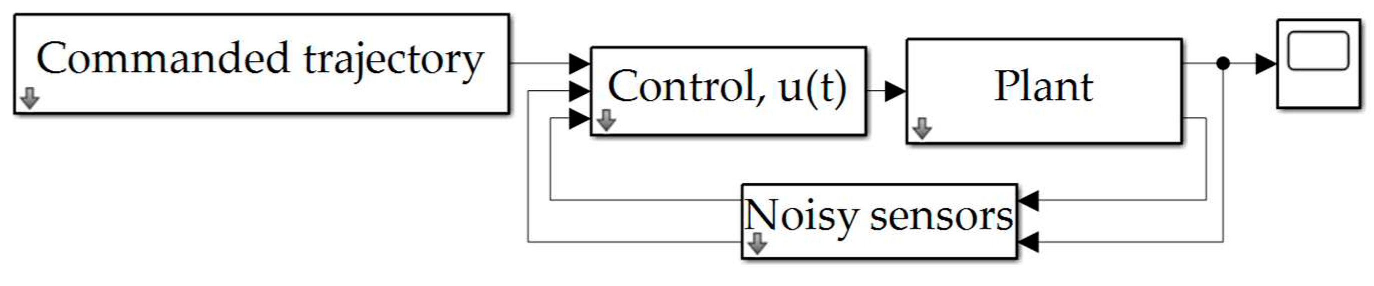
Figure A2.
MATLAB® simulation of commanded trajectory options.
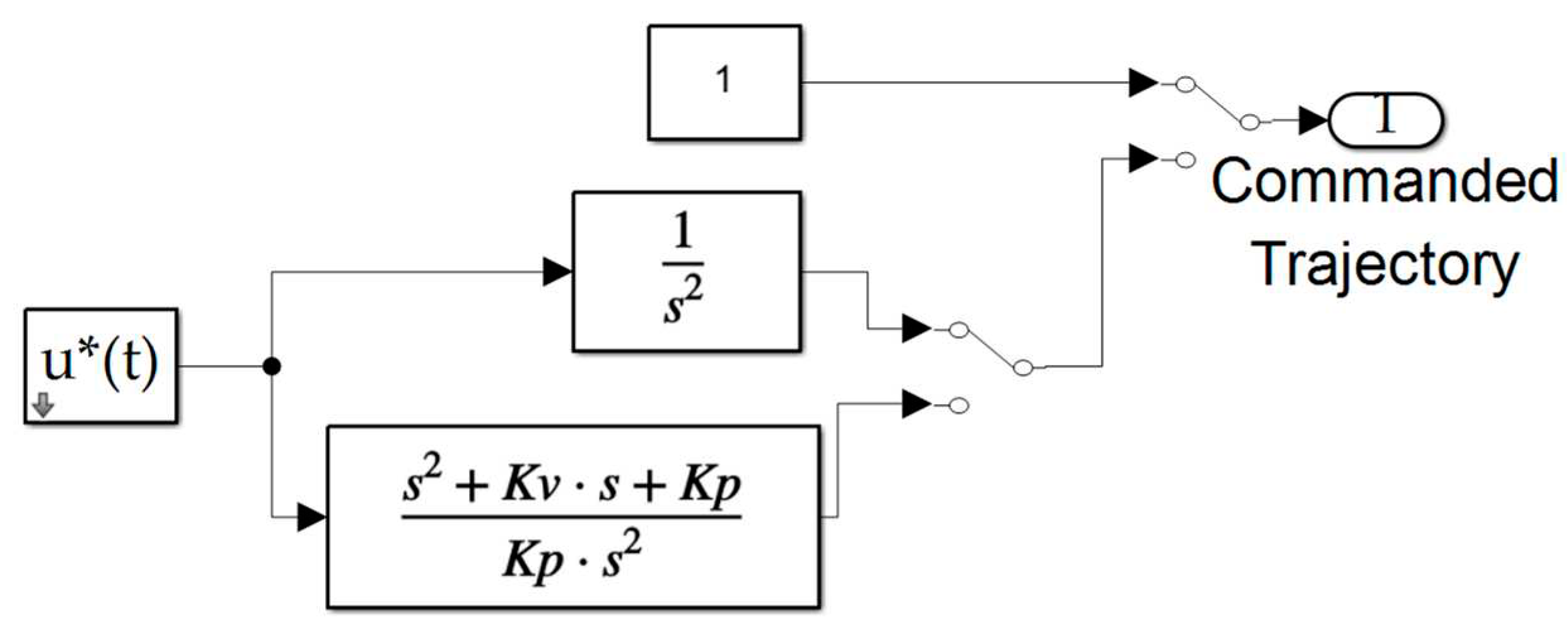
Figure A3.
MATLAB® simulation of controller options.
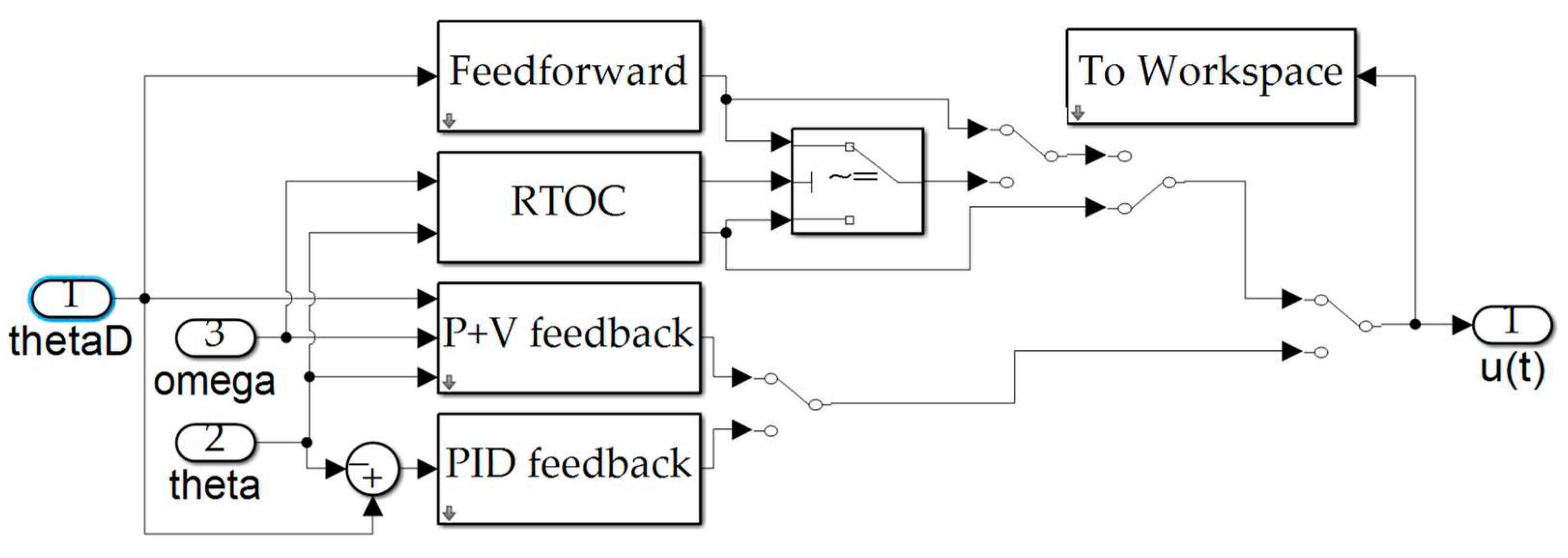
Figure A4.
MATLAB® simulation of (a) feedforward control calculation, (b) P+V control.
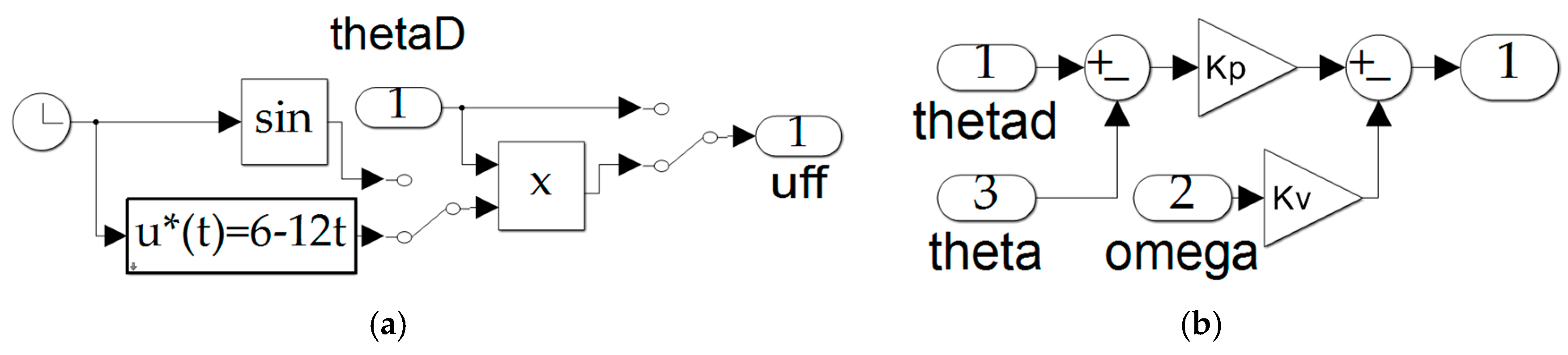
Figure A5.
MATLAB® simulation of real-time optimal control.
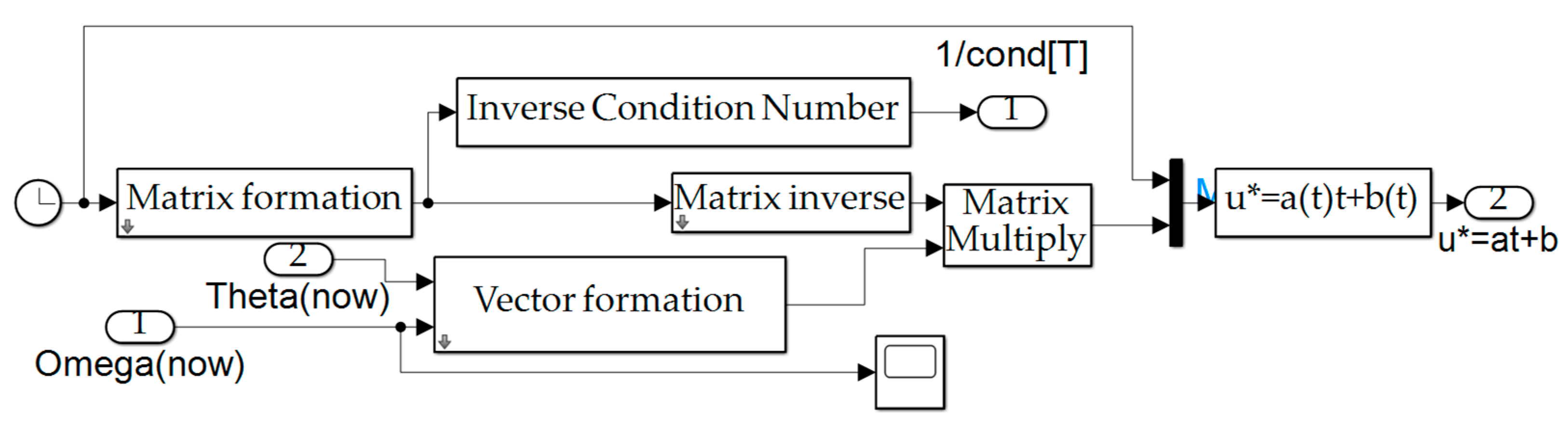
Figure A6.
MATLAB® simulation of (a) PID feedback control calculation, (b) Plant.
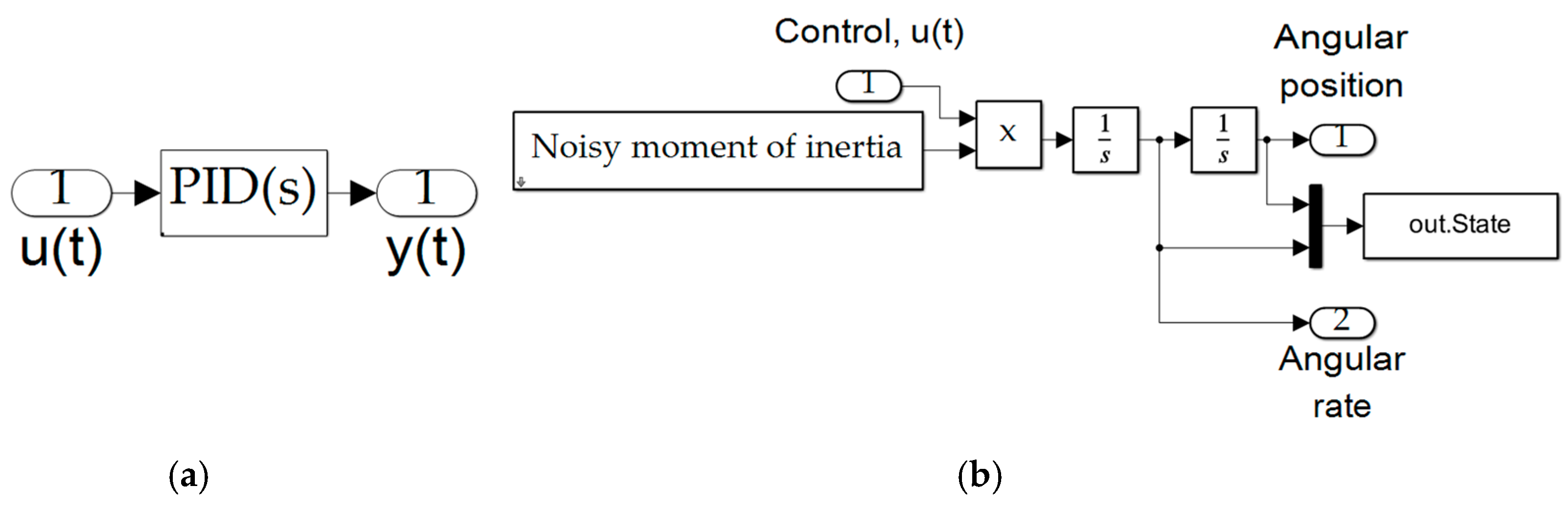
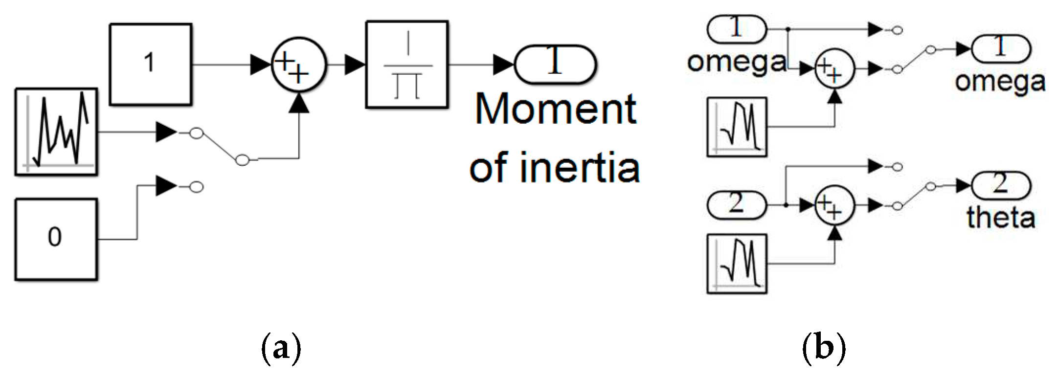
Figure A7.
MATLAB® simulation of (a) noisy moment of inertia calculation, (b) noisy sensors.
Appendix B
Definitions of variables and nomenclature
Table B1.
| Variables | Definitions | Variables | Definitions |
|---|---|---|---|
| Angle | the quadratic cost functional | ||
| Angular velocity | The dynamic cost function | ||
| Rotational acceleration | The dynamic constraint | ||
| The inertia of moment | System torque | ||
| The initial time | The final time | ||
| u | Control function on time | t | Time(dimensionless) |
| The Hamilton equation | The dynamic cost function | ||
| , | The Lagrangian | The dynamic constraint | |
| The Lagrangian about x | The derivative of Lagrangian | ||
| x | System states | The derivative of states | |
| The total end-point cost | The static cost function | ||
| The static constraint function | The torque from the controller | ||
| Lagrange multiplier about | Lagrange multiplier about | ||
| The derivative about the lagrangian | The derivative about the lagrangian | ||
| s | Complex variable for Laplace Transform | a, b, c | Constants of integration |
| The desired transformed angle | The actual velocity (the velocity output with the noise) | ||
| The desired torque input | The actual angle (the position output with the noise) | ||
| The noise from the position sensor | The noise from the velocity sensor | ||
| The desired angle | The input of the control structure (angle) | ||
| The desired control | The output of the control structure (control) |
References
- Rakhimjon Shokirov. Prospects of the Development of Unmanned Aerial Vehicles (UAVs). Technical Science and Innovation 2020, Volume 2020, Issue 3.
- Apurv Saha; Akash Kumar. FPV drone with GPS used for surveillance in remote areas. 2017 Third International Conference on Research in Computational Intelligence and Communication Networks (ICRCICN). Kolkata, India, 03-05 November 2017. 05 November.
- Upasita Jain; Marcus Rogers. Drone forensic framework: Sensor and data identification and verification. 2017 IEEE Sensors Applications Symposium (SAS). Glassboro, USA, 13-15 March 2017. 15 March.
- Patrick Black, NASA Offer Guidance for Drone Use Viewing Antares Launch, 2021, Available online: https://www.nasa.gov/wallops/2021/press-release/nasa-offers-guidance-for-drone-use-viewing-antares-launch.
- NASA. NASA Image Use Policy. 2022. Available online: https://gpm.nasa.gov/image-use-policy (accessed on 14 April 2023).
- UM. Rao. Mogili; B.B. Deepak. Review on Application of Drone Systems in Precision Agriculture. ELSEVIER 2018. Vol. 133, pp.502-509.
- Marthinus Reinecke; Tania Prinsloo. The influence of drone monitoring on crop health and harvest size. 2017 1st International Conference on Next Generation Computing Applications (NextComp). Mauritius. 19-21 July 2017.
- Faris. A. Almalkl; Maha Aljohani. Incorporating Drone and AI to Empower Smart Journalism via Optimizing a Propagation Model. MDPI 2022. 14 (7), 3758. [CrossRef]
- G. Quiroz; S. J. Kim. A Confetti Drone: Exploring Drone Entertainment. 2017 IEEE International Conference on Consumer Electronics (ICCE). Las Vegas, USA, 08-10 January 2017.
- Chong Huang; Zhenyu Yang. Learning to Capture a Film-Look Video with a Camera Drone. 2019 International Conference on Robotics and Automation (ICRA). Montreal, Canada, 20-24 May 2019.
- Ansias Carmona. Eduardo. Development of active camera stabilization system for implementation on UAV’s, Bachelor thesis, Polytechnic University of Catalonia, Spain, 2012.
- Nguyen Cong Danh. The Stability of a Two-Axis Gimbal System for the Camera. Hindawi 2021, Volume 2021.
- Mateo Gasparovic; Luka Jurjevic. Gimbal Influence on the Stability of Exterior Orientation Parameters of UAV Acquired Images. Sensors 2017, 17, 401.
- M. Kim; G.S. Byun; G.H. Kim. The stabilizer design for a drone-mounted camera gimbal system using intelligent-PID controller and used and tuned mass damper. International. Journal of Control and Automation 2016, Volume 9, pp. 397-394.
- R. J. Rajesh and C. M. Ananda, "PSO tuned PID controller for controlling camera position in UAV using 2-axis gimbal," 2015 International Conference on Power and Advanced Control Engineering (ICPACE), Bengaluru, India, 2015, pp. 128-133.
- Qianwen Duan;Xi Zhou. Pointing control design based on the PID type-III control loop for two-axis gimbal systems. ELSEVIER 2021. Vol. 331, 112923.
- Miroslav. LASSAK. Small UAV Camera Gimbal Stabilization Using Digital Filters and Enhanced Control Algorithms for Aerial Survey and Monitoring. Acta Montanistica Slovaca 2020, Vol. 25, pp. 127-137.
- Altan; R.Hacioglu. Model predictive control of three-axis gimbal system mounted on UAV for real-time target tracking under external disturbances, Mechanical Systems and Signal Processing 2020, Vol. 138.
- W., Aguilar; C. Angulo. Real-Time Model-Based Video Stabilization for Microaerial Vehicles. Neural Processing Letters 2015. Vol. 43, pp. W. Aguilar; C. Angulo. Real-Time Model-Based Video Stabilization for Microaerial Vehicles. Neural Processing Letters 2015. Vol. 43, pp. 459-477.
- V. Kangunde; Rodrigo S. Jamisola Jr. A review on drones controlled in real-time International. Journal of Dynamics and Control 2021, Vol. 9, pp. 1832-1846.
- Altan; R. Hacioglu. Real-Time Control based on NARX Neural Network of Hexarotor UAV with Load Transporting System for Path Tracking. 2018 6th International Conference on Control Engineering & Information Technology (CEIT). Istanbul, Turkey. 2018, pp. 1-6.
- Haeun Yoo; Boeun Kim. Reinforcement learning based optimal control of batch process using Monte Carlo deep deterministic policy gradient with phase segmentation. ELSEVIER 2021, Vol. 144, 107133.
- K. Binder. Applications of Monte Carlo Methods to statistical physics, Reports on Progress in Physics 1997, Vol. 60, 487.
- Timothy Sands. Inducing Performance of Commercial Surgical Robots in Space. Sensors 2023, 23, 1510.
- Ekkaphon Mingkhwan; Weerawat Khawsuk. Digital image stabilization technique for fixed camera on small size drone. 2017 Third Asian Conference on Defense Technology (ACDT). Phuket, Thailand, 2021.
- Jean-Luc Guermond; Murtazo Nazarov. Second-Order Invariant Domain Preserving Approximation of the Euler Equations Using Convex Limiting. Society for Industrial and Applied Mathematics (SIAM) 2018. Vol. 40, Iss. 5. [CrossRef]
- Shushen Qin, Marcus Cramer. Optimal control for Hamiltonian parameter estimation in non-commuting and bipartite quantum dynamics. SciPost Physics 2022. 13. 121.
- Tim Breitenbach; Alfio Borzi. A Sequential Quadratic Hamiltonian Method for Solving Parabolic Optimal Control Problems with Discontinuous Cost Functionals. Journal of Dynamical and Control Systems 2019. Vol. 25, pp. 403-435.
- M. A. Jafarizadeh; F. Naghdi. Time optimal control of two-level quantum systems. ELSEVIER 2020. Vol. 384, 29.
- D. Alpago; F. Dorfler. An Extended Kalman Filter for Data-Enabled Predictive Control. IEEE Control Systems Letters 2020. Vol. 4, pp. 994-999.
- Michael Ross. A Primer on Pontryagin’s Principle in Optimal Control, 2nd ed; E. Solon; Collegiate Publishers, San Francisco, Carmel, 2022.
- Zhi-Cheng Yang; Armin Rahmani. Optimizing Variational Quantum Algorithms Using Pontryagin’s Minimum Principle. PHYSICAL REVIEW X 2017, Vol. 7, Iss. 2.
- Yeqin Wang; Wu Zhen. Research on energy optimization control strategy of the hybrid electric vehcle based on Pontryagin’s minimum principle. ELSEVIER 2018. Vol. 72, pp. 203-213.
- Hanane Dagdougui; Ahmed Ouammi. Optimal Control of a Network of Power Microgrids Using the Pontryagin’s Minimun Principle. IEEE Transactions on Control Systems Technology 2014. Vol. 22, Iss. 5.
Disclaimer/Publisher’s Note: The statements, opinions and data contained in all publications are solely those of the individual author(s) and contributor(s) and not of MDPI and/or the editor(s). MDPI and/or the editor(s) disclaim responsibility for any injury to people or property resulting from any ideas, methods, instructions or products referred to in the content. |
© 2023 by the authors. Licensee MDPI, Basel, Switzerland. This article is an open access article distributed under the terms and conditions of the Creative Commons Attribution (CC BY) license (http://creativecommons.org/licenses/by/4.0/).
Copyright: This open access article is published under a Creative Commons CC BY 4.0 license, which permit the free download, distribution, and reuse, provided that the author and preprint are cited in any reuse.


