Submitted:
12 May 2023
Posted:
15 May 2023
You are already at the latest version
Abstract
In this paper, under the symmetric entropy and the scale squared error loss functions, we consider the maximum likelihood (ML) estimation and Bayesian estimation of the Shannon entropy and Rényi entropy of the two-parameter inverse Weibull distribution. In the ML estimation, the dichotomy is used to solve likelihood equation. In addition, the approximation confidence interval is given by the Delta method. Because the form of estimation results is more complex in the Bayesian estimation, the Lindley approximation method is used to achieve the numerical calculation. Finally, Monte Carlo simulations and a real data set are used to illustrate the results derived. By comparing the mean square error between the estimated value and the real value, it can be found that the performance of ML estimation of Shannon entropy is better than that of Bayesian estimation, and there is no significant difference between the performance of ML estimation of Rényi entropy and that of Bayesian estimation.
Keywords:
Inverse Weibull distribution
; symmetric entropy loss function
; Rényi entropy
; Bayesian estimation
; Lindley approximation
MSC: 62F10; 62F15
1. Introduction
Information is an abstract concept. In the face of a large amount of data, it is easy to know how much data there is, but it is not clear how much information this data contain. Entropy is one of the important terms in physics. Shannon [1] introduced the concept of entropy into statistics, which represents the uncertainty of events. This entropy is generally called “Shannon entropy”. Generally speaking, when we hear a message within expectation, we think it contains less information. When we hear an unexpected message, we think that the amount of information it conveys to us is huge. In statistics, the probability is usually used to describe the uncertainty of an event. Therefore, Shannon believes that probability can be used to describe the amount of information contained in an event. After that, Alred Rényi [2] generalized Shannon entropy and put forward the concept of Rényi entropy. Since then, the study of entropy has attracted a lot of attention [3,4]. For example, Chacko and Asha [5] considered the maximum likelihood (ML) estimation and Bayesian estimation of Shannon entropy for generalized exponential distribution by the importance sampling method based on record values. Liu and Gui [6] considered the ML estimation and Bayesian estimation of Shannon entropy for two-parameter Lomax distribution by the Lindley method and the Tierney-Kadane method under a generalized progressively hybrid censoring test. Shrahili et al. [7] considered the estimation of entropy of Log-Logistic distribution. The estimations of different entropy functions are obtained by the ML method, and the approximate confidence intervals are obtained by using various censoring methods and sample sizes. Mahmoud et al. [8] considered the estimation of entropy and residual entropy of two-parameter Lomax distribution based on the generalized type-II hybrid censoring scheme. The ML estimators and Bayesian estimators of entropy and residual entropy are obtained. The simulation study of estimating performance under different sample sizes is described. Finally, the conclusion is discussed. Hassan and Mazen [9] estimated three entropy measures for the inverse Weibull distribution using progressively Type-II censored data, which are Shannon entropy, Rényi entropy, and q-entropy. The method of maximum likelihood and maximum product of spacing are used to estimate them. Mavis et al. [10] proposed and studied gamma-inverse Weibull distribution, and some mathematical properties were given including moments, mean deviations, Bonferroni and Lorenz curves, and entropies. Basheer [11] introduced a new generalized alpha power inverse Weibull distribution, and the Shannon entropy and Rényi entropy were obtained. Valeriia and Broderick [12] proposed the weighted inverse Weibull class of distributions and derived the expressions of Shannon entropy and Rényi entropy.
In 1982, Keller and Kamath [13] introduced the Inverse Weibull Distribution (IWD) to model the degradation of mechanical components of diesel engines. It is a useful lifetime probability distribution, and it can be used to represent various failure characteristics. Depending on the value of the shape parameter of the IWD, the risk function can be changed flexibly. The use of IWD for data fitting is therefore more appropriate in many cases. For example, Abhijit and Anindya [14] found that the use of IWD was superior to previous normal models when measuring concrete structures using ultrasonic pulse velocities. Chiodo et al. [15] proposed a new model generated from an appropriate mixture of IWD for modeling extreme wind speed scenarios. Langlands et al. [16] observed that breast cancer mortality data could be analyzed using IWD for modeling analysis. That is why two-parameter IWD has attracted more and more researchers to pay attention to and discuss in recent years [17,18]. For example, Asuman and Mahmut [19] considered the classical and Bayesian estimation of parameters and the reliability function of the IWD. In classical estimation, they derived the ML estimators and modified ML estimators. In Bayesian estimation, they utilized the Lindley method to calculate the Bayesian estimators of parameters under symmetric and asymmetric loss functions. Sultan et al. [20] discussed the estimation of parameters of IWD based on the progressive type-II censored sample. They put forward an approximate maximum likelihood method to obtain the ML estimator and used Lindley's approximation to obtain the Bayesian estimators. Amirzadi et al. [21] considered the Bayesian estimation of scale parameter and reliability in the inverse generalized Weibull distribution. In addition to general entropy, squared log error, and weight squared error function. They introduced a new loss function to carry out Bayesian estimation. Peng and Yan [22] studied the Bayesian estimation and prediction for shape and scale parameters of the IWD under a general progressive censoring test. Sindhu et al. [23] assumed different priors and loss functions, and discussed the Bayesian estimation of inverse Weibull mixture distributions based on doubly censored data. Mohammad and Sana [24] obtained the Bayes estimators and ML estimators for the unknown parameters of IWD under lower record values. Faud [25] developed a linear exponential loss function, and estimated parameter and reliability of IWD based on lower record values under this loss function. Li and Hao [26] considered the estimation of a stress-strength model when stress and strength are two independent IWDs with different parameters. Ismail and Tamimi [27] proposed a constant stress partially accelerated life test model and analyzed it using type-I censored data from IWD. Kang and Han [28] derived the approximate maximum likelihood estimators of parameters of IWD under multiply type-II censoring and also proposed a simple graphical method for a goodness-on-fit test. Saboori et al. [29] introduced generalized modified inverse Weibull distribution, and some statistical and probabilistic properties were derived.
This paper will consider the Bayesian estimation of Shannon entropy and Rényi entropy of two-parameter IWD based on complete samples. In Section 2, some related knowledge is introduced first, and then the specific expressions of Shannon entropy and Rényi entropy of two-parameter IWD are derived. In Section 3, the maximum likelihood estimators of the scale parameter and shape parameter of IWD are derived by the dichotomy method, and then the ML estimators of Shannon entropy and Rényi entropy are obtained. In Section 4, the gamma distribution is adopted as the prior distribution (PD) of the scale parameter. A non-informative PD is adopted as the PD of the shape parameter. And then the Bayesian estimators of Shannon entropy and Rényi entropy are obtained based on the symmetric entropy loss function and scale squared error loss function. Lindley approximation is used to achieve the numerical calculation of the Bayesian estimators of entropy, on account of the complexity of these Bayesian estimators. In Section 5, Monte Carlo simulations are utilized to simulate and compare the estimators that are mentioned above. In Section 6, a real data set has been analyzed for illustrative purposes. Finally, the conclusions of the article are given in Section 7.
2. Preliminary Knowledge
The probability density function (pdf) of two-parameter IWD is defined as Eq. (1).
and the cumulative distribution function (cdf) of two-parameter IWD is defined as Eq. (2)
where the scale parameter is , and the shape parameter is .
Figure 1 shows the pdf of IWD under different values of shape and scale parameters, respectively.
The Shannon entropy is defined in Equation (Eq. 3) [1]
and the Rényi entropy is defined in Equation (Eq. 4) [2]
where is the pdf of a continuous random variable .
Theorem 1.
Letis a random sample that follows IWD with the pdf (1),are the sample observations of.
(i) Shannon entropy of IWD is showed in Eq. (5)
(ii) Rényi entropy of IWD is showed in Eq. (6)
where the gamma function and is Euler constant.
Proof. The log density of pdf (1) of IWD is showed in Eq. (7)
According to the log-density function (7), and Eq. (3), the Shannon entropy of IWD can be derived as follows:
Obviously,
Let ,
Because
Let ,
Therefore, Shannon entropy of two-parameter IWD can be expressed as
Obviously,
Then, according to Eq. (4), the Rényi entropy of two-parameter IWD can be expressed as
3. Maximum Likelihood Estimation
Suppose that is a random sample that follows IWD with the pdf (1), are the sample observations of . Thus, the likelihood function (LF) can be derived as Eq. (8)
Then, the corresponding log LF of Eq. (8) is showed in Eq. (9)
For convenience, we denote as . Thus, the likelihood equations can be expressed respectively as Eq. (10) and Eq. (11)
The ML estimators and can be obtained by solving Eq. (10) and Eq. (11) with dichotomy, whose calculation steps are listed as follows:
(i) According to Eq. (10) and Eq. (11), there are
(ii) Denote , given the accuracy , determine the interval and verify .
(iii) Find the midpoint of the interval and calculate .
(iv) If , .
(v) If , ; If , .
(vi) If , is equal to or . If not, return to step (iii) to step (vi).
Due to the invariance of ML estimation, the ML estimators of Shannon entropy and Rényi entropy can be obtained by putting and into Eq. (3) and Eq. (4), and their mathematical expressions are showed in Eq. (14) and Eq. (15)
Next, the Delta method is used to derive the approximate confidence intervals (briefly, ACIs) of Shannon entropy and Rényi entropy.
Denote vectorandas
in whichandare calculated through Eq. (18) and Eq. (19).
According to the Delta method, calculate the estimated variance ofandas Eq. (20) and Eq. (21).is the Fisher information matrix ofand, and Eq. (22) gives the elements of. is the inverse matrix of.
Then, theACI of Shannon entropy is Eq. (23), and theACI of Rényi entropy is Eq. (24), whereis the upper ()th quantile of the standardized normal distribution.
4. Bayesian Estimation
Bayesian estimation is a method of introducing prior information to deal with decision problems. The advantage is that it can include the prior information in statistical inference and improve the accuracy of the taken decision. From the time when Bayesian estimation was proposed to now, many researchers have adopted this method in estimating parameters and related functions. For example, Kundu and Howlader [30] considered the Bayesian inference and prediction of inverse Weibull distribution, based on type-II censored data. A Gibbs sampling procedure was used for MCMC samples, and Bayes estimation was computed by this sample. Sultan et al. [31] considered the Bayesian estimation of inverse Weibull parameters based on progressive type-II censored data. Because the Bayes estimators can’t be obtained explicitly, the Lindley approximation was used to calculate them. Mohammad and Mina [32] presented the Bayesian inferences of parameters of inverse Weibull distribution based on type-I hybrid censored data and computed the Bayes estimates using Lindley approximation. Algarni et al. [33] considered the Bayes estimation of parameters for the inverse Weibull distribution employing a progressive type-I censored sample. Metropolis-Hasting (MH) algorithm was used to compute the Bayesian estimates.
In addition to the areas mentioned above, there are some recent applications of the Bayesian method. Zhou and Luo [34] developed a supplier's recursive multiperiod discounted profit model based on Bayesian information updating. Yulin et al. [35] put forward a Bayesian approach to tackle the misalignments for over-the-air computation. Taborsky et al. [36] presented a novel generic Bayesian probabilistic model to solve the problem of parameters marginalization under the constraint of forced community structure. Oliver [37] introduced the Bayesian toolkit and showed how geomorphic models might benefit from probabilistic concepts. Ran et al. [38] proposed a Bayesian approach to measure the loss of privacy in a mechanism. Luo et al. [39] used the Bayesian information criterion for model selection when revisiting the lifetime data of brake pads. Peng et al. [40] extended a general Bayesian framework to deal with the degradation analysis of sparse degradation observations and evolving observations. František et al. [41] illustrated Bayesian estimation of how to benefit parametric survival analysis. Liu et al. [42] proposed fuzzy Bayesian knowledge tracing models to address continuous score scenarios.
In this paper, the Bayesian estimations of Shannon entropy and Rényi entropy of IWD are investigated under symmetric entropy (SE) and scale squared error (SSE) loss functions, which are widely used in Bayesian statistical inference [43,44,45].
(i) SE loss function is defined in Equation (Eq. 25) [43]
where is the estimator of .
Lemma 1. Suppose that is the historical data information about the entropy function . Then, under the SE loss function (25), the Bayesian estimator for any prior distribution is showed in Eq. (26)
where is the posterior expectation of and is the posterior expectation of .
Proof. Under the SE loss function (25), the Bayesian risk of is
To minimize , only need to minimize . For convenience, let.
Because
and the derivative is
The Bayesian estimator can be obtained by .
(ii) SSE loss function is defined in Equation (Eq. 27) [45]
where is a nonnegative integer.
Lemma 2. Suppose that is the historical data information about the entropy function . Then, under the SSE loss function (27), the Bayesian estimator for any prior distribution is
where is the posterior expectation of and is the posterior expectation of .
Proof. Under the SSE loss function (27), the Bayesian risk of is
To minimize , only need to minimize . Similarly, let .
Because
and the derivative of is
The Bayes estimator can be obtained by .
Assume that the scale parameter and shape parameter of two-parameter IWD are independent random variables, which obey and obey non-informative PD as follows:
Thus, the joint PD of and is
Referring to Bayesian formulation, the posterior distribution of and is
Thus, the Bayesian estimators of Shannon entropy and Rényi entropy under SE can be expressed as
The Bayesian estimators of Shannon entropy and Rényi entropy under SSE can be expressed as
From Eq. (33) to Eq. (36), it can be seen that the calculation of Bayesian estimators of Shannon and Rényi entropy are complex and difficult to calculate. Thus, Lindley approximation will be employed to achieve the approximate calculation results of and .
4.1. Bayesian Estimation by using Lindley approximation under SE loss function
Referring to Lindley approximation, can be defined as
where is a function of independent variables and , is log LF defined in Eq. (9), is the log of joint PD defined in Eq. (31).
If the sample size is large, Eq. (37) can be expressed as
where and are the ML estimators of and , and
() is the element of inverse matrix of .
The is denoted that taking the second derivative of with respect to and putting into it. Similarly, others can be expressed as
Under the SE loss function, the step of numerical calculation of Shannon entropy by Lindley approximation is shown as follows:
When ,
Put Eq. (40) and Eq. (41) into Eq. (38), is obtained.
Similarly, when ,
Then, put Eq. (40) and Eq. (42) into Eq. (38), is obtained. Thus, the numerical calculation of Shannon entropy is calculated by Eq. (33).
Under the SE loss function, the numerical calculation of Rényi entropy by Lindley approximation is shown as follows:
When ,
Put Eq. (40) and Eq. (43) into Eq. (38), is obtained.
When ,
Put Eq. (40) and Eq. (44) into Eq. (38), is obtained. Thus, the numerical calculation of Shannon entropy is calculated by Eq. (34).
4.2. Bayesian Estimation by using Lindley approximation under SSE loss function
Under the SSE loss function, the step of numerical calculation of Shannon entropy by Lindley approximation is shown as follows:
When ,
Then, putting Eq. (40) and Eq. (45) into Eq. (38), is obtained.
When ,
Then, putting Eq. (40) and Eq. (46) into Eq. (38), is obtained. Thus, the numerical calculation of Shannon entropy is calculated by Eq. (35).
Under the SSE loss function, the step of numerical calculation of Rényi entropy by Lindley approximation is shown as follows:
When ,
Put Eq. (40) and Eq. (47) into Eq. (38),is obtained.
When,
Put Eq. (40) and Eq. (48) into Eq. (38), is obtained. Thus, the numerical calculation of Rényi entropy is calculated by Eq. (36).
5. Monte Carlo simulation
In this chapter, Monte Carlo simulation is used to generate random samples that obey two-parameter IWD, and repeat 1000 experiments respectively with different sample sizes (). The true values of the parameters in the two-parameter IWD are taken as and , the parameters of the gamma distribution are taken as and , the parameters in SSE are taken as , and the parameters of the Rényi entropy are taken as . Then, the mean squared error (briefly, MSE) is used to compare the performance of each estimator. The results of Shannon entropy are shown in Table 1, and the results of Rényi entropy are shown in Table 2. For showing the performance of ACIs, the coverage probability is calculated and the results are shown in Table 3.
For convenience, and represent the true values of Shannon entropy and Rényi entropy, and represent mean values of 1000 ML estimates of entropy respectively, and represent mean values of 1000 Bayesian estimates of entropy respectively under SE loss function, and represent mean values of 1000 Bayesian estimates of entropy respectively under SSE loss function, and represent MSEs of ML estimates of entropy respectively, and represent MSEs of Bayesian estimates of entropy respectively under SE loss function, and represent MSEs of Bayesian estimates of entropy respectively under SSE loss function. The and () are calculated by Eq. (49) and Eq. (50), where and represents the i-th ML estimate or Bayesian estimate of Shannon entropy. The and () are calculated by Eq. (51) and Eq. (52), where and represents the i-th ML estimate or Bayesian estimate of Rényi entropy.
Based on the above tables, the following conclusions can be drawn:
(1) For Shannon entropy, the ML estimation performs better than the Bayesian estimation. While for Rényi entropy, the performance of ML estimation is similar to Bayesian estimation.
(2) In Bayesian estimation, it is better to select the SE to estimate Shannon entropy. On the contrary, it is better to select the SSE to estimate Rényi entropy.
(3) The sample size has a great influence on Shannon entropy than Rényi entropy. When the sample size increases gradually, the Bayesian estimation of Shannon entropy under SE is close to the ML estimation, but it has no obvious effect on Rényi entropy.
(4) In Table 3, it can be noted that the coverage probability of ACIs is quite close to confidence levels.
6. Real data analysis
There is a real data set given by Bjerkdal [46], which represents the survival time (in days) of guinea pigs after the injection of different doses of tubercle bacilli. Kundu and Howlader [47] proved that this set of data sets using the IWD fitting effect is very good, therefore, this data set can be seen as a sample of IWD. In Reference [46], the regimen number refers to the common logarithm of bacillary units contained in 0.5 ml of challenge solution. In other words, regimen 6.6 represents 4.0*106 bacillary units per 0.5 ml. Corresponding to regimen 6.6, the 72 observed observations are listed as follows:
12, 15, 22, 24, 24, 32, 32, 33, 34, 38, 38, 43, 44, 48, 52, 53, 54, 54, 55, 56, 57, 58, 58, 59, 60, 60, 60, 60, 61, 62, 63, 65, 65, 67,68, 70, 70, 72, 73, 75, 76, 76, 81, 83, 84, 85, 87, 91, 95, 96, 98, 99, 109, 110, 121, 127, 129, 131, 143, 146, 146, 175, 175, 211,233, 258, 258, 263, 297, 341, 341, 376.
Using the proposed estimates described in the above sections, the ML estimates and Bayesian estimates of Shannon entropy and Rényi entropy are displayed in Table 4. It’s obvious that the ML estimates of entropies are all smaller than Bayesian estimates under SE respectively, and the Bayesian estimates under SSE of entropies are all smaller than ML estimates respectively.
7. Conclusions
This paper considers the Bayesian estimations of Shannon entropy and Rényi entropy based on two-parameter IWD. First, the expressions of these entropies of two-parameter IWD are derived in Theorem 1. For ML estimation, due to the invariance of ML estimation, the ML estimators of parameters are obtained by the dichotomy method at first. And then, the ML estimators of entropies can be obtained. Additionally, the approximate confidence intervals are given by the Delta method. For Bayesian estimation, the symmetric entropy loss function and scale squared error loss function are chosen. However, the forms of Bayesian estimators are complex and difficult to calculate. Lindley approximation is used to solve this problem. Finally, the mean square errors of the above estimators are used to compare their performances. For Shannon entropy, it’s better to use ML estimator. And for Rényi entropy, the performances of the ML estimator and Bayesian estimator are analogous.
Author Contributions
Conceptualization, H.P. and X.H.; methodology, H.P.; software, X.H.; validation, H.P. and X.H.; writing—original draft preparation, X.H.; writing—review and editing, H.P.; funding acquisition, H.P. All authors have read and agreed to the published version of the manuscript.
Funding
This research was funded by National Natural Science Foundation of China, grant number 71661012.
Data Availability Statement
Not applicable.
Conflicts of Interest
The authors declare no conflict of interest.
References
- Shannon, C. E. A mathematical theory of communication. Bell. Labs. Tech. J. 1948, 27, 379–423. [Google Scholar] [CrossRef]
- Rényi, A. On measures of entropy and information. Berkeley Symp on Math. Statist. and Prob. 1970, 4, 547–561. [Google Scholar]
- Alexander Bulinsk; Denis Dimitrov. Statistical estimation of the Shannon entropy. Acta Math Sin 2019, 35, 17–46. [Google Scholar] [CrossRef]
- Wolf Ramona. Information and entropies. Lect Notes Phys 2021, 988, 53–89. [Google Scholar]
- Chacko, M.; Asha, P. S. Estimation of entropy for generalized exponential distribution based on record values. J. Indian Soc. Prob. St. 2018, 19, 79–96. [Google Scholar] [CrossRef]
- Liu, S.; Gui, W. Estimating the entropy for Lomax distribution based on generalized progressively hybrid censoring. Symmetry 2019, 11, 1–17. [Google Scholar] [CrossRef]
- Shrahili, M.; El-Saeed, A.R.; Hassan, A.S.; Elbatal, I. Estimation of entropy for Log-Logistic distribution under progressive type II censoring. J. Nanomater 2022, 3, 1–10. [Google Scholar] [CrossRef]
- Mahmoud, M.R.; Ahmad, M.A.M.; Mohamed, B.S.Kh. Estimating the entropy and residual entropy of a Lomax distribution under generalized type-II hybrid censoring. Math. Stat. 2021, 9, 780–791. [Google Scholar] [CrossRef]
- Hassan, O.; Mazen, N. Product of spacing estimation of entropy for inverse Weibull distribution under progressive type-II censored data with applications. J. Taibah Univ. Sci. 2022, 16, 259–269. [Google Scholar]
- Mavis, P.; Gayan, W. L.; Broderick, O. O. A New Class of Generalized Inverse Weibull Distribution with Applications. J Appl Math Bioinformatics 2014, 4, 17–35. [Google Scholar]
- Basheer, A. M. Alpha power inverse Weibull distribution with reliability application. J Taibah Univ Sci 2019, 13, 423–432. [Google Scholar] [CrossRef]
- Valeriia, S.; Broderick, O. O. Weighted Inverse Weibull Distribution: Statistical Properties and Applications. Theor Math Appl 2014, 4, 1–30. [Google Scholar]
- Keller A Z; Kamath A R R. Alternative reliability models for mechanical systems. 3rd International Conference on Reliability and Maintainability, Toulose, France, 1982.
- Abhijit, C; Anindya, C. Use of the Fréchet distribution for UPV measurements in concrete. NDT E Int. 2012, 52, 122–128. [Google Scholar] [CrossRef]
- Chiodo, E; Falco, P D; Noia, L P D; Mottola, F. Inverse loglogistic distribution for Extreme Wind Speed modeling: Genesis, identification and Bayes estimation. AIMS Energy 2018, 6, 926–948. [Google Scholar] [CrossRef]
- A O Langlands; S J Pocock; G R Kerr; S M Gore. Long-term survival of patients with breast cancer: a study of the curability of the disease. Brit Med J 1979, 2, 1247–1251. [Google Scholar] [CrossRef] [PubMed]
- Ellah, A. Bayesian and non-Bayesian estimation of the inverse Weibull model based on generalized order statistics. Intell Inf Manag 2012, 4, 23–31. [Google Scholar]
- Singh, S K; Singh, U; Kumar, D. Bayesian estimation of parameters of inverse Weibull distribution. J Appl Stat 2013, 40, 1597–1607. [Google Scholar] [CrossRef]
- Asuman, Y.; Mahmut, K. Reliability estimation and parameter estimation for inverse Weibull distribution under different loss functions. Kuwait J. Sci. 2022, 49, 1–24. [Google Scholar]
- Sultan, K.S.; Alsadat, N.H.; Kundu, D. Bayesian and maximum likelihood estimations of the inverse Weibull parameters under progressive type-II censoring. J. Stat. Comput. Sim. 2014, 84, 2248–2265. [Google Scholar] [CrossRef]
- Amirzadi, A.; Jamkhaneh, E.B.; Deiri, E. A comparison of estimation methods for reliability function of inverse generalized Weibull distribution under new loss function. J. Stat. Comput. Sim. 2021, 91, 2595–2622. [Google Scholar] [CrossRef]
- Peng, X.; Yan, Z. Z. Bayesian estimation and prediction for the inverse Weibull distribution under general progressive censoring, Commu. Stat.- Theor. M. 2016, 45, 621–635. [Google Scholar]
- Sindhu, T. N; Feroze, N; Aslam, M. Doubly censored data from two-component mixture of inverse Weibull distributions: Theory and Applications. J. Mod. Appl. Stat. Meth. 2016, 15, 322–349. [Google Scholar] [CrossRef]
- Mohammad, F.; Sana, S. Bayesian estimation and prediction for the inverse Weibull distribution based on lower record values. J. Stat. Appl. Probab. 2021, 10, 369–376. [Google Scholar]
- Faud, S. Al-Duais. Bayesian analysis of Record statistic from the inverse Weibull distribution under balanced loss function. Math. Probl. Eng. 2021, 2021, 1–9. [Google Scholar] [CrossRef]
- Li, C.P.; Hao, H.B. . Reliability of a stress-strength model with inverse Weibull distribution. Int. J. Appl. Math. 2017, 47, 302–306. [Google Scholar]
- Ismail, A.; Al Tamimi, A. Optimum constant-stress partially accelerated life test plans using type-I censored data from the inverse Weibull distribution. Strength Mater 2017, 49, 847–855. [Google Scholar] [CrossRef]
- Kang, S.B.; Han, J.T. The graphical method for goodness of fit test in the inverse Weibull distribution based on multiply type-II censored samples. SpringerPlus 2015, 4, 768. [Google Scholar] [CrossRef] [PubMed]
- Saboori, H.; Barmalzan, G.; Ayat, S.M. Generalized modified inverse Weibull distribution: Its properties and applications. Sankhya B 2020, 82, 247–269. [Google Scholar] [CrossRef]
- Debasis Kundu; Hatem Howlader. Bayesian inference and prediction of the inverse Weibull distribution for Type-II censored data. Comput Stat Data Anal 2010, 54, 1547–1558. [Google Scholar] [CrossRef]
- Sultan, K.S.; Alsadat, N.H.; Kundu, D. . Bayesian and maximum likelihood estimations of the inverse Weibull parameters under progressive type-II censoring. J Stat Comput Simul 2014, 84, 2248–2265. [Google Scholar] [CrossRef]
- Mohammad K; Mina A. Estimation of the Inverse Weibull Distribution Parameters under Type-I Hybrid Censoring. Austrian J. Stat. 2021, 50, 38–51. [Google Scholar] [CrossRef]
- Ali Algarni; Mohammed Elgarhy; Abdullah M Almarashi; Aisha Fayomi; Ahmed R El-Saeed. Classical and Bayesian Estimation of the Inverse Weibull Distribution: Using Progressive Type-I Censoring Scheme. Adv. Civ. Eng. 2021, 2021, 1–15. [Google Scholar] [CrossRef]
- Zhou, J.H.; Luo, Y. Bayes information updating and multiperiod supply chain screening. Int J Prod Econ 2023, 256, 108750–108767. [Google Scholar] [CrossRef]
- Yulin, S; Deniz, G; Soung, C L. Bayesian Over-the-Air Computation. IEEE J. Sel. Areas Commun. 2023, 41, 589–606. [Google Scholar] [CrossRef]
- Taborsky, P; Vermue, L; Korzepa, M; Morup, M. The Bayesian Cut. IEEE Trans. Pattern Anal. Mach. Intell. 2021, 43, 4111–4124. [Google Scholar] [CrossRef] [PubMed]
- Oliver Korup. Bayesian geomorphology. Earth Surf Process Landf. 2021, 46, 151–172. [Google Scholar] [CrossRef]
- Ran, E; Kfir, E; Mu, X. S. Bayesian privacy. Theor. Econ. 2021, 16, 1557–1603. [Google Scholar] [CrossRef]
- Luo, C.L.; Shen, L.J.; Xu, A.C. Modelling and estimation of system reliability under dynamic operating environments and lifetime ordering constraints. Reliab. Eng. Syst. Saf. 2022, 218, 108136–108145. [Google Scholar] [CrossRef]
- Peng, W. W.; Li, Y. F.; Yang, Y. J.; Mi, J. H.; Huang, H.Z. Bayesian Degradation Analysis With Inverse Gaussian Process Models Under Time-Varying Degradation Rates. IEEE Trans Reliab 2017, 66, 84–96. [Google Scholar] [CrossRef]
- František, B; Frederik, A; Julia, M. H. Informed Bayesian survival analysis. BMC Medical Res. Methodol. 2022, 22, 238–260. [Google Scholar] [CrossRef]
- Liu, F.; Hu, X.G.; Bu, C.Y.; Yu, K. Fuzzy Bayesian Knowledge Tracing. IEEE Trans Fuzzy Syst 2022, 30, 2412–2425. [Google Scholar] [CrossRef]
- Xu, B.; Wang, D.H.; Wang, R.T. Estimator of scale parameter in a subclass of the exponential family under symmetric entropy loss. Northeast. Math. J. 2008, 24, 447–457. [Google Scholar]
- Li, Q.; Wu, D. Bayesian analysis of Rayleigh distribution under progressive type-II censoring. J. Shanghai Polytech. Univ. 2019, 36, 114–117. [Google Scholar]
- Song, L.X.; Chen, Y.S.; Xu, J.M. Bayesian estimation of Pission distribution parameter under scale squared error loss function. J. Lanzhou Univ. Tech. 2008, 34, 152–154. [Google Scholar]
- Bjerkdal, Tor. Acquisition of resistance in guinea pigs infected with different doses of virulent tubercle bacilli. Am J Epidemiol, 1960, 72, 130–148. [Google Scholar] [CrossRef]
- Debasis Kundu; Hatem Howlader. Bayesian inference and prediction of the inverse Weibull distribution for Type-II censored data. Comput Stat Data An 2010, 54, 1547–1558. [Google Scholar] [CrossRef]
Figure 1.
The curves of the pdf of IWD with respect to different values of parameters.
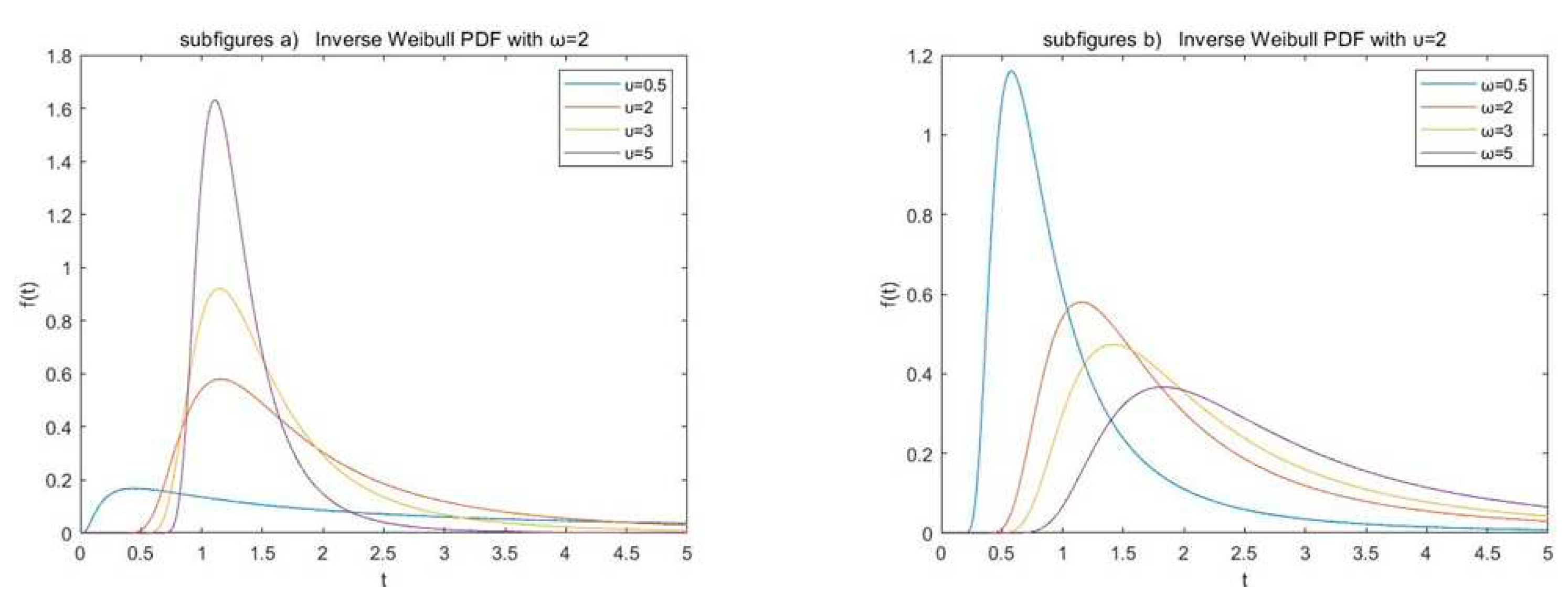

Table 1.
Estimates and MSEs of Shannon entropy ().
| Sample size () | Estimate | MSE | ||||
| 10 | 1.0604 | 0.8259 | 0.8914 | 0.1903 | 0.3666 | 0.2065 |
| 20 | 1.1183 | 0.9631 | 0.9683 | 0.0863 | 0.1282 | 0.1186 |
| 30 | 1.1388 | 1.0301 | 1.0076 | 0.0558 | 0.0751 | 0.0766 |
| 40 | 1.1355 | 1.0526 | 1.0292 | 0.0445 | 0.0574 | 0.0592 |
| 50 | 1.1461 | 1.0788 | 1.0379 | 0.0323 | 0.0404 | 0.0472 |
| 60 | 1.1503 | 1.0938 | 1.0506 | 0.0287 | 0.0343 | 0.0399 |
| 70 | 1.1579 | 1.1093 | 1.0646 | 0.0244 | 0.0282 | 0.0334 |
| 80 | 1.1623 | 1.1196 | 1.0694 | 0.0197 | 0.0224 | 0.0284 |
| 90 | 1.1653 | 1.1272 | 1.0803 | 0.0171 | 0.0191 | 0.0256 |
| 100 | 1.1628 | 1.1284 | 1.0777 | 0.0161 | 0.0183 | 0.0244 |
Table 2.
Estimates and MSEs of Rényi entropy ().
| Sample size () | Estimate | MSE | ||||
| 10 | 1.6681 | 1.7793 | 1.7682 | 0.0525 | 0.1075 | 0.0954 |
| 20 | 1.6056 | 1.6512 | 1.6587 | 0.0178 | 0.0218 | 0.0186 |
| 30 | 1.5999 | 1.6278 | 1.6229 | 0.0129 | 0.0136 | 0.0112 |
| 40 | 1.5903 | 1.6113 | 1.6082 | 0.0103 | 0.0103 | 0.0075 |
| 50 | 1.5829 | 1.5992 | 1.5972 | 0.0072 | 0.0071 | 0.0064 |
| 60 | 1.5809 | 1.5954 | 1.5896 | 0.0055 | 0.0057 | 0.0049 |
| 70 | 1.5765 | 1.5885 | 1.5878 | 0.0046 | 0.0046 | 0.0045 |
| 80 | 1.5781 | 1.5886 | 1.5857 | 0.0044 | 0.0041 | 0.0034 |
| 90 | 1.5752 | 1.5845 | 1.5779 | 0.0038 | 0.0038 | 0.0032 |
| 100 | 1.5731 | 1.5814 | 1.5775 | 0.0032 | 0.0032 | 0.0031 |
Table 3.
The coverage probability of ACIs with different .
| Sample size() | Shannon entropy | Rényi entropy | ||
| 10 | 0.9637 | 0.9752 | 0.9662 | 0.9791 |
| 20 | 0.9798 | 0.9894 | 0.9789 | 0.9884 |
| 30 | 0.9829 | 0.9916 | 0.9847 | 0.9930 |
| 40 | 0.9839 | 0.9941 | 0.9860 | 0.9953 |
| 50 | 0.9857 | 0.9946 | 0.9894 | 0.9957 |
| 60 | 0.9876 | 0.9947 | 0.9936 | 0.9954 |
| 70 | 0.9875 | 0.9947 | 0.9925 | 0.9965 |
| 80 | 0.9875 | 0.9940 | 0.9929 | 0.9972 |
| 90 | 0.9894 | 0.9955 | 0.9934 | 0.9966 |
| 100 | 0.9865 | 0.9950 | 0.9929 | 0.9971 |
Table 4.
The estimates and ACIs of entropies based on the real data set.
| ML estimates | Bayesian estimates | ACIs | |||
| Under SE | Under SSE | ||||
| Shannon entropy | 5.6307 | 5.6998 | 4.8706 | (5.1858, 6.0757) | (5.1328, 6.1287) |
| Rényi entropy | 5.4129 | 4.7280 | 4.8706 | (5.1877, 5.6381) | (5.1609, 5.6649) |
Disclaimer/Publisher’s Note: The statements, opinions and data contained in all publications are solely those of the individual author(s) and contributor(s) and not of MDPI and/or the editor(s). MDPI and/or the editor(s) disclaim responsibility for any injury to people or property resulting from any ideas, methods, instructions or products referred to in the content. |
© 2023 by the authors. Licensee MDPI, Basel, Switzerland. This article is an open access article distributed under the terms and conditions of the Creative Commons Attribution (CC BY) license (http://creativecommons.org/licenses/by/4.0/).
Copyright: This open access article is published under a Creative Commons CC BY 4.0 license, which permit the free download, distribution, and reuse, provided that the author and preprint are cited in any reuse.


