Submitted:
14 May 2023
Posted:
15 May 2023
You are already at the latest version
Abstract
Selecting the optimal activation function for training deep neural networks has always been challenging because it significantly impacts the neural network’s performance and training speed. At this point, researchers are more likely to employ RELU than other well-known activation functions. After RELU, researchers have proposed many activation functions to improve RELU. None of them was capable of surpassing RELU as their most significant rival. SWISH outperformed RELU in several challenging experiments like classification, object detection, and tracking. Replacing RELU units with SWISH, which improves performance in many tasks. This paper proposed a new activation function surpassing Google’s brain’s SWISH function, Which we named AIF. Experiments indicate that our proposed activation function outperforms SWISH in various tasks.
Keywords:
Activation Function
; Neural Network
; Deep Learning
; RELU
; SWISH
1. Introduction
During the training of a neural network, the primary process occurring in each neuron is a linear transformation followed by an activation function. The importance of the activation function in deep network training is inevitable [1,2].
Listed below are some of the most prevalent types of activation functions for neural networks:
1.1. Binary Step
The presence of a threshold value is used to determine whether a neuron should become active. A threshold is evaluated concerning the activation function input to determine whether a neuron’s input should trigger the function. The input must be greater than the threshold for the neuron to become active. If the input is lower than the threshold, the neuron’s output will not pass on to the next hidden layer. Equation 1 expresses this function:
However, the binary step function is not without its limitations. First, it cannot generate outputs with multiple values; for instance, we cannot use this function to solve classification problems involving multiple classes since zero gradients of the step function impede the backpropagation procedure.
1.2. Linear
The output of the linear activation function is proportional to the input. This activation function is also known as the "no activation function" or the "identity function." This function returns its input value and does not modify its arguments’ weighted sum. This function is expressed mathematically as:
Nevertheless, a linear activation function has two significant drawbacks. Because the function’s derivative is constant and has no relationship with the input x, backpropagation would have no effect. Additionally, if each neuron uses a linear activation function, all neural network layers will collapse into one. The output of a neural network’s final layer will always be a linear function of the input of the first layer, regardless of how many layers the network has. Because of this, a neural network can be simplified down to a single layer when each neuron uses a linear activation function.
The linear activation function is just a regression model. This linear regression model cannot be used to generate intricate maps between the network’s inputs and outputs due to its limited capabilities. We can circumvent the limitations inherent to linear activation functions by employing their non-linear analogs, known as non-linear activation functions. Since the derivative function depends on the input, they make it possible to perform backpropagation. To be more exact, they make it feasible to figure out which weights in the input neurons will predict more precisely. Moreover, the utilization of non-linear activation functions makes it possible to stack multiple layers of neurons, which in turn causes the output to be a non-linear combination of the inputs from each stacked layer. This results in the output being a non-linear combination of the inputs.
1.3. Sigmoid
This function accepts any real value as its input and will always return a value between 0 and 1. As demonstrated below, the output value will be closer to 1 if the input value is greater and closer to 0 if the input value is smaller. We can express this function mathematically as:
Users frequently employ this function in models that require a probability prediction as an output. Given that the probability of anything exists only between 0 and 1, the sigmoid distribution is the best option. The function can differentiate and has a continuous gradient, preventing output value jumps. The sigmoid activation function is an S-shaped curve. The sigmoid function has certain constraints. Sigmoid function derivative is expressed mathematically as:
The only region of the sigmoid graph where the gradient values are meaningful is from -3 to 3, and the rest of the graph becomes much flatter. Hence the gradients of the function will be extremely minimal for values greater than 3 or less than -3. Vanishing gradients will occur when the value of the gradient gets near zero because the network will stop learning at that point. As the value gets closer to zero, the output of the logistic function starts to behave asymmetrically. As a consequence of this, the output of every neuron will always have the same sign. Consequently, training the neural network will become difficult and more likely to become unstable.
1.4. Hyperbolic Tangent
The TANH function is extremely comparable to the sigmoid and logistic activation functions. It even has the same S-shaped output range, which varies from -1 to 1. When using Tanh, the output value will be closer to 1.0 when the input value is larger and closer to -1.0 when the input value is smaller. Equation 5 represents the TANH function:
The output of the TANH activation function is zero-centered. Consequently, it is simple to map output values as either strongly negative, neutral, or strongly positive. Second, because its values can range from -1 to 1, it is frequently utilized in the hidden layers of a neural network. Consequently, the hidden layer’s mean value is either 0 or an extremely close approximation of that value. This attribute helps center the data and simplifies learning the next layer parameters.
TANH gradients tend to converge to zero. Additionally, the TANH function’s gradient is noticeably more critical than the gradient of the sigmoid function. TANH is zero-centered, so vanishing gradients can go in any direction they like, unlike sigmoid, which has a fixed gradient direction. Therefore, when it comes to practical applications, TANH non-linearity is always preferred over sigmoid non-linearity.
1.5. RELU
RELU is a computationally efficient function with a suitable derivative for backpropagation. Not all neurons are activated concurrently by the RELU function. Deactivation of the neurons will occur if the output of the linear transformation is negative and greater than 0. Equation 6 represents the RELU function:
Since the sigmoid and TANH functions activate a much larger number of neurons than the RELU function, which only activates a small number of neurons, the RELU function is significantly more computationally efficient. In addition, the fact that RELU is linear and does not saturate speeds up the convergence of gradient descent to the global minimum of the loss function because the loss function does not reach its maximum value during the process. However, there are some restrictions associated with using this function. The gradient value is zero on the negative side of the graph.
For this reason, the backpropagation process would not update some neuron weights, which can cause neurons to become permanently inactive, known as dying neurons. As a direct result, the model’s capacity to correctly fit the data or learn from it would diminish due to the immediate conversion of all negative input values to zero.
1.6. Leaky RELU
Leaky RELU is a more advanced variant of the RELU function developed to solve the problems caused by Dying neurons which is caused by having a modestly positive slope in the negative region of the function’s domain. Equation 7 expresses Leaky RELU:
The benefits of using Leaky RELU are identical to those of RELU; the only difference is that Leaky RELU enables backpropagation even for values with negative inputs. The gradient on the left side of the graph will move away from zero and into the positive territory when this straightforward adjustment for negative input values happens. As a direct result, we would no longer find dead neurons in that particular region. The following are some limitations placed on this function. Negative Input values could lead to inaccurate predictions. Because negative values have such a low gradient, discovering new model parameters takes much more time.
1.7. Parametric RELU
Parametric RELU is a form of RELU produced to address the zero gradients along the axis’s left side. Equation 8 represents RELU:
Where is the parameter that determines the slope for negative values, the effectiveness of this function might change for various problems according to the value entered into the slope parameter.
1.8. Exponential Linear Units
The Exponential Linear Unit is an alternative to the RELU that changes the slope of the function’s negative portion. In contrast to leaky RELU and parametric RELU, which both use a straight line to define negative values, ELU uses a log curve instead. Equation 9 represents the ELU function :
ELU becomes smooth gradually, while RELU becomes smooth abruptly. The log curve for negative input values eliminates the dying RELU problem. It assists the network in adjusting the weights and biases in the appropriate direction. The time required to complete the computation increased due to the exponential operation. Moreover, no learning of the function hyperparameter - - takes place. Exploding gradient problem is another main problem for ELU.
1.9. SELU
In self-normalizing networks, SELU is the function that would take care of internal normalization. Using this function, we could guarantee that each layer would maintain the same mean and variance as the layers that preceded it. SELU makes this normalization process easier by adjusting the mean and the variance. On the other hand, the SELU activation function can shift the mean using both positive and negative values. In contrast, the RELU activation function cannot output negative values and, therefore, cannot shift the mean. Equation 10 represents the SELU function:
SELU has predefined alpha and lambda values. The primary advantage that SELU possesses in comparison to RELU is since internal normalization occurs quicker than external normalization, the network can converge faster. SELU is a relatively new activation function that needs additional research on CNNs and RNNs, among other architectures.
1.10. SOFTMAX
This activation function is built based on a sigmoid(logistic) activation function. Equation 11 represents the SOFTMAX function:
The SOFTMAX function is a combination of several different sigmoid functions. It computes the proportional probabilities. In a manner analogous to the sigmoid (logistic) activation function, the SOFTMAX activation function also returns the probability associated with each class. In the case of multiclass classification, practitioners widely employ it as an activation function for the final layer of a neural network.
For instance, if we are to assume that there are three different classes, then the output layer would have three neurons. Consider for a moment that the output of the neurons is the following: [1.8, 0.9, 0.68]. If we want a probabilistic perspective, we can apply the SOFTMAX function to these values, producing the following result: [0.58, 0.23, 0.19]. The function will return 1 for the array index corresponding to the probability with the highest value and 0 for the other two array indexes since the probability with the highest value corresponds to the array index receiving the highest value. In this case, index 0 is given the same weight as indexes 1 and 2, which receive no weight. The class that would be output as a result would be the one that corresponds to the first neuron (index 0) out of the three.
1.11. SWISH
Google researchers developed this self-gated activation function. The SWISH activation function consistently matches or outperforms the RELU activation function on deep neural networks applied to challenging domains. This function is constrained below, but unconstrained above, which means that Y will approach a constant value as X approaches negative infinity. Still, as X approaches infinity, Y will approach infinity. Moreover, the SWISH function is constrained below but unconstrained above. Equation 12 represents this function:
SWISH is significantly more advantageous than RELU in several respects. SWISH is a smooth function, indicating that it does not suddenly shift direction at x = 0 as RELU does. Instead, SWISH follows a smooth curve that descends from 0 to values that are less than 0 before rising again. Secondly, within the RELU activation function, any negative values that were lower than a predetermined threshold will be nullified. Despite this, these negative values could help determine the data’s underlying patterns.
The non-monotonic nature of the SWISH activation function makes it possible for a more accurate expression of the input data and the weight that needs to be learned by training.
At this point, the most widely used activation function is RELU [3,4,5,6], defined as f(x) = max(x,0). RLEU outperforms many other ones, such as sigmoid and TANH, because it can overcome some previous problems, such as vanishing gradients. The use of RELU was a breakthrough that enabled the fully supervised training of state-of-the-art deep networks [7]. Deep neural networks that use RELU in their heart are more optimized than networks with sigmoid or TANH units [8]. Researchers have proposed numerous activation functions to replace RELU [9,10,11,12] but none of them were as successful as SWISH [8].With the introduction of SWISH, many practitioners started to favor SWISH over RELU because of its simplicity, reliability, and consistent performance improvement across different models and datasets. Figure 1 shows the abovementioned activation functions.
In This paper, we proposed a new activation function surpassing Google’s brain’s SWISH function, which we named AIF. Our extensive experiments on various datasets and architectures indicate that replacing SWISH units with AIF units accelerates the training speed and improves classification accuracy.
2. The proposed activation function
Although the above-mentioned Activation Functions work well, they have two main drawbacks: computational complexity and performance issue. None of them overcome the SWISH activation function in deep neural network architecture. In this paper, we proposed a new activation function called Active Identity Function (AIF). AIF is a non-linear and smooth function. We express AIF mathematically as:
where a is a hyperparameter as below:
Our extensive experiments show that AIF consistently matches or outperforms SWISH on deep neural networks applied to various challenging tasks on multiple architectures. For example, on ImageNet [13], AIF acts as consistent as SWISH but replacing SWISH units with AIF units leads to convergence speed acceleration; with SWISH units, the network converges after 43 epochs, but with AIF units, network converges after 12 epochs.
As shown in Figure 2, when x tends to be Infinite positive, AIF tends to be the identity function. On the other hand, when x tends to be an Infinite negative, AIF tends to be . Moreover, Figure 3 illustrates the AIF activation function and its first derivative behavior while using various amounts of .
Like SWISH, AIF is Non-linear, which makes AIF proven to be a universal function approximator. While both SWISH and AIF are both unbonded above, AIF is unbonded below if . The unboundedness property prevents the neural network from saturation [14].
However, for , it is bounded below, where the gradients of AIF are negative. This may also be advantageous because of strong regularization effects [8]. AIF is smooth and continuously differentiable. For our activation function, when x is close to 0, is close to 0. The AIF and its first/second derivatives are shown in equation 13, 15, and, 16, respectively.
Figure 4 shows the graph of the first and second derivatives of AIF.
3. Experimental results
In this section, we benchmark AIF against SWISH. This widely used activation function consistently outperforms RELU or matches it on challenging datasets. We illustrate that AIF reaches or exceeds SWISH on nearly all tasks. In our experiments, we have chosen if else 0.1. The following sections will describe our experimental settings and results in greater detail.
3.1. Datasets
To evaluate AIF, we use Cifar [15], MNIST[16], and ImageNet [13] datasets. These datasets have been used by many similar works and the community to elaborate the proposed methods. Therefore, In the rest of this section, we will investigate the datasets mentioned above regarding their size, sample types, special features, etc.
3.1.1. Cifar10
The CIFAR-10 dataset (Canadian Institute For Advanced Research) [15] is a collection of frequently used images to train machine learning and computer vision algorithms. The Canadian Institute For Advanced Research created this dataset. It is one of the datasets that is utilized the most frequently in the field of machine learning research. The CIFAR-10 dataset includes sixty thousand color images with a resolution of 32 by 32 pixels, organized into ten different categories. The ten distinct classes each represent a different type of vehicle, including airplanes, automobiles, birds, cats, deer, dogs, frogs, horses, and trucks. There are six thousand pictures belonging to each category.
3.1.2. MNIST
The MNIST database [16], which stands for the Modified National Institute of Standards and Technology database, is a sizable collection of handwritten digits frequently utilized for training various image processing systems. The database is frequently utilized in machine learning for training and testing. There are 60,000 images used for training in the MNIST database, and another 10,000 are used for testing.
3.1.3. ImageNet
ImageNet [13] is a database of images structured according to the WordNet hierarchy (at the moment, only the nouns are included), and each node of the hierarchy is represented by anywhere from hundreds to thousands of images. Research in computer vision and deep learning has advanced significantly as a direct result of the project. Researchers are welcome to use the data for any purpose other than commercial gain without incurring costs.
3.2. Caps Net on cifar10
Caps Net [17] is an acronym for a specific type of neural network presented by Stanford scientist Jeffrey Hinton. In Caps Net, a unique method is used for image processing to try to affect the perception of objects in the three-dimensional spectrum.
In other words, the Caps Net neural network is a machine learning system to model hierarchical relationships better. This approach is an attempt to mimic biological neural organization.
The idea is to add structures called capsules to a convolutional neural network (CNN)[18] and reuse the output of multiple capsules to create more stable profiles (due to different abnormalities) for higher capsules. Now we train the Caps Net network on the cifar10 [19] data with AIF and the SWISH activation function. Figure 6 indicates the graph of network accuracy on the cifar10 dataset using these two activation functions. As can be seen, network training and testing with AIF work slightly better than the SWISH activation function.
3.3. Net2Net
Researchers often create different neural network architectures in traditional machine learning work and try to improve the current model. After training a model , the next architecture starts training from the beginning (random startup). In other words, it means losing all the information from the previous model. The Net2Net [19] technique speeds up the testing process by instantly transferring knowledge of a prior network to any newer or deeper network. Net2Net methods work based on the change in performance maintenance between neural network specifications. We now evaluate Net2Net on two sets of cifar10 and MNIST datasets with AIF and the SWISH activation function.
3.3.1. Net2Net on Cifar
According to Figure 6, the accuracy chart on the CIFAR10 data with the two activation functions indicates that AIF performed better than the SWISH with a slight difference.
3.3.2. Net2Net on MNIST
3.4. Transfer learning on ImageNet data
Figure 9 shows the training diagram of transfer learning [20] on ImageNet data with AIF and SWISH activation functions. We used the MobileNet architecture [21] in Transfer learning. As can be seen in Figure 9, the network with AIF has reached its maximum accuracy in less time compared to the network with the SWISH activation function.
3.5. ResNet20_v1 on cifar10
Microsoft introduced the network, which stands for Residual Network[22]. In this network, some communications are considered between layers to transfer inputs from previous layers to the next without intermediaries. Outside of the convolutional structure, In the backward propagation [23] or correction stage, the error of each layer is transferred to the last layer so that the network can be deepened and trained faster. This architecture, with a depth of 152 layers, is one of the deepest architectures, according to Figure 9; the ResNet20_v1 network with AIF result’s 85% training accuracy in training and 80% accuracy of validation data. It performs slightly better than the SWISH activation function, with 82.5% and 78% accuracy and validation accuracy, respectively.
3.6. Convolutional Neural Network on MNIST Data
Here we train a convolutional neural network with the MNIST data, which contains images of handwritten digits, with AIF and SWISH activation functions. Figure 10 illustrates the evaluation results. As can be seen, AIF performed better than the SWISH activation function, comparing the training accuracy and the validation data.
We collected the results in Table 1 by comparing the performance of AIF to the SWISH activation function applied to various models across multiple datasets.
4. Discussion
Our extensive experiments show that AIF consistently performs better than the SWISH function on mentioned tasks. Proving an activation function’s superiority over another is challenging due to many conditions that affect the training process. AIF is a non-linear, monotonic (when ), smooth, continuously differentiable, and unbounded above and below (when ) function, which does not approximate identity near the origin but still has a convex surface error. With , although AIF is non-monotonic, the error surface will remain convex. Furthermore, smooth functions with a convex error on derivatives will generalize better.
AIF is easily computable, and we can implement it within a single line of code in most deep learning libraries such as TensorFlow [24] and PyTorch [25](e.g.,).
One important aspect of activation functions is how they propagate gradients through the network. Imagine we have a very deep neural network with more than 50 layers. The gradients for the input layer, i.e. the very first layer, have passed times the activation function, but we still want them to be of a reasonable size. If the gradient through the activation function is (in expectation) considerably smaller than 1, gradients will vanish until they reach the input layer. If the gradient through the activation function is larger than 1, the gradients exponentially increase and might explode. Figure 11 illustrates the way activation functions propagate gradients through the network by showing gradient magnitude for SWISH, RELU and AIF respectively. Furthermore, AIF is a zero-centered function that overcomes the vanishing gradient problem and enables fast convergence for deep networks, as shown in the experiments.
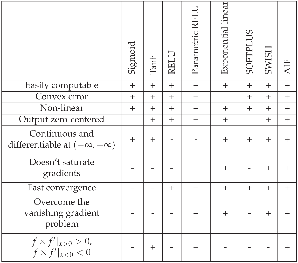
As we mentioned earlier, one of the brilliant properties of AIF is the error convexity. Table 2 compares our proposed function with some widely used functions; many of these activation functions do not satisfy this mathematical condition.The output values range of AIF is infinite. This property makes AIF more efficient, so that pattern representations significantly affect most weights.
Order of continuity until First-order parametric continuity () is an advantage for every activation function, which is vital because the neural network uses the activation function’s first prime in the weight correction process during back-propagation.
Not only does AIF satisfy this property, but also it satisfies the order of continuity until second-order parametric continuity () This means that our activation function’s first prime is continuously differentiable. This property is a brilliant feature that makes our activation function distinctive from other known activation functions.
Although AIF does not approximate identity near the origin, it preserves the good weights, which means for points close to zero, the gradient of our activation function is close to zero too. AIF is very sensible and understandable. From the mathematical point of view, it estimates identity function nonlinearly (i.e. )
5. Conclusion
We have proposed an activation function that we refer to as AIF. Several experiments have shown that this activation function performs well in various architectural contexts and datasets. In addition, the AIF satisfies the essential requirements that an activation function should have. These essential requirements are non-linearity, smoothness, infinite range, monotonicity, zero-centered, rapid convergence, overcoming vanishing gradient, avoiding gradient saturation, error convexity, rapid computation, easy implementation, and continuous and differentiable values. Our exhaustive experiments showed that AIF is superior to Google’s brain’s SWISH.
References
- W. S. McCulloch and W. Pitts, “A logical calculus of the ideas immanent in nervous activity,” The bulletin of mathematical biophysics, vol. 5, no. 4, pp. 115–133, 1943. [CrossRef]
- Y. LeCun, Y. Y. LeCun, Y. Bengio, and G. Hinton, “Deep learning,” nature, vol. 521, no. 7553, pp. 436–444, 2015. [CrossRef]
- A. F. arXiv:1803.08375, Feb. 2019. [CrossRef]
- R. H. R. Hahnloser, R. R. H. R. Hahnloser, R. Sarpeshkar, M. A. Mahowald, R. J. Douglas, and H. S. Seung, “Digital selection and analogue amplification coexist in a cortex-inspired silicon circuit,” Nature, vol. 405, pp. 947–951, Jun. 2000. [Google Scholar] [CrossRef]
- K. Jarrett, K. K. Jarrett, K. Kavukcuoglu, M. Ranzato, and Y. LeCun, “What is the best multi-stage architecture for object recognition?,” in 2009 IEEE 12th International Conference on Computer Vision, Sep. 2009, pp. 2146–2153. [CrossRef]
- V. Nair and G. E. Hinton, “Rectified Linear Units Improve Restricted Boltzmann Machines,” presented at the ICML, Jan. 2010. Accessed: Jun. 14, 2022. [Online].
- V. Nair and G. E. Hinton, “Rectified Linear Units Improve Restricted Boltzmann Machines,” presented at the ICML, Jan. 2010. Accessed: Jun. 14, 2022. [Online].
- P. Ramachandran, B. P. Ramachandran, B. Zoph, and Q. V. arXiv:1710.05941, Oct. 2017. [CrossRef]
- A. L. Maas, A. Y. A. L. Maas, A. Y. Hannun, and A. Y. Ng, “Rectifier nonlinearities improve neural network acoustic models,” in Proc. icml, 2013, vol. 30, no. 1, p. 3.
- K. He, X. K. He, X. Zhang, S. Ren, and J. Sun, “Delving Deep into Rectifiers: Surpassing Human-Level Performance on ImageNet Classification,” presented at the Proceedings of the IEEE International Conference on Computer Vision, 2015, pp. 1026–1034. Accessed: Jun. 14, 2022. [Online].
- D.-A. Clevert, T. D.-A. Clevert, T. Unterthiner, and S. arXiv:1511.07289, Feb. 2016. [CrossRef]
- G. Klambauer, T. G. Klambauer, T. Unterthiner, A. Mayr, and S. Hochreiter, “Self-Normalizing Neural Networks,” in Advances in Neural Information Processing Systems, 2017, vol. 30. Accessed: Jun. 14, 2022. [Online].
- J. Deng, W. J. Deng, W. Dong, R. Socher, L.-J. Li, K. Li, and L. Fei-Fei, “ImageNet: A large-scale hierarchical image database,” in 2009 IEEE Conference on Computer Vision and Pattern Recognition, Jun. 2009, pp. 248–255. [CrossRef]
- X. Glorot and Y. Bengio, “Understanding the difficulty of training deep feedforward neural networks,” in Proceedings of the Thirteenth International Conference on Artificial Intelligence and Statistics, Mar. 2010, pp. 249–256. Accessed: Jun. 14, 2022. [Online].
- A. Krizhevsky and G. Hinton, “Learning multiple layers of features from tiny images,” 2009.
- L. Deng, “The mnist database of handwritten digit images for machine learning research [best of the web],” IEEE signal processing magazine, vol. 29, no. 6, pp. 141–142, 2012.
- S. Sabour, N. S. Sabour, N. Frosst, and G. E. arXiv:1710.09829, Nov. 2017. [CrossRef]
- Y. LeCun and Y. Bengio, “Convolutional networks for images, speech, and time series,” The handbook of brain theory and neural networks, vol. 3361, no. 10, p. 1995, 1995.
- T. Chen, I. T. Chen, I. Goodfellow, and J. A: Shlens, “Net2net; arXiv:1511.05641, 2015.
- S. Bozinovski, “Reminder of the first paper on transfer learning in neural networks, 1976,” Informatica, vol. 44, no. 3, 2020. [CrossRef]
- A. G. Howard et al. E: “Mobilenets; arXiv:1704.04861, 2017. [CrossRef]
- K. He, X. K. He, X. Zhang, S. Ren, and J. Sun, “Deep residual learning for image recognition,” in Proceedings of the IEEE conference on computer vision and pattern recognition, 2016, pp. 770–778.
- H. J. Kelley, “Gradient theory of optimal flight paths,” Ars Journal, vol. 30, no. 10, pp. 947–954, 1960. [CrossRef]
- M. Abadi et al., “TensorFlow: A System for Large-Scale Machine Learning,” presented at the 12th USENIX Symposium on Operating Systems Design and Implementation (OSDI 16), 2016, pp. 265–283. Accessed: Jun. 14, 2022. [Online].
- A. Paszke et al., “PyTorch: An Imperative Style, High-Performance Deep Learning Library,” in Advances in Neural Information Processing Systems, 2019, vol. 32. Accessed: Jun. 14, 2022. [Online].
Figure 1.
Diagram of Common Activation Functions and their first derivative. a: Diagrams of Binary Step, Linear, Sigmoid, Tanh, and SWISH activation functions. b: Diagrams of RELU, leaky RELU, Parametric RELU, SELU, and Exponential Linear Unit. c: indicates the first order derivative of the functions mentioned in a. d: illustrates the first order derivative of the functions mentioned in b.
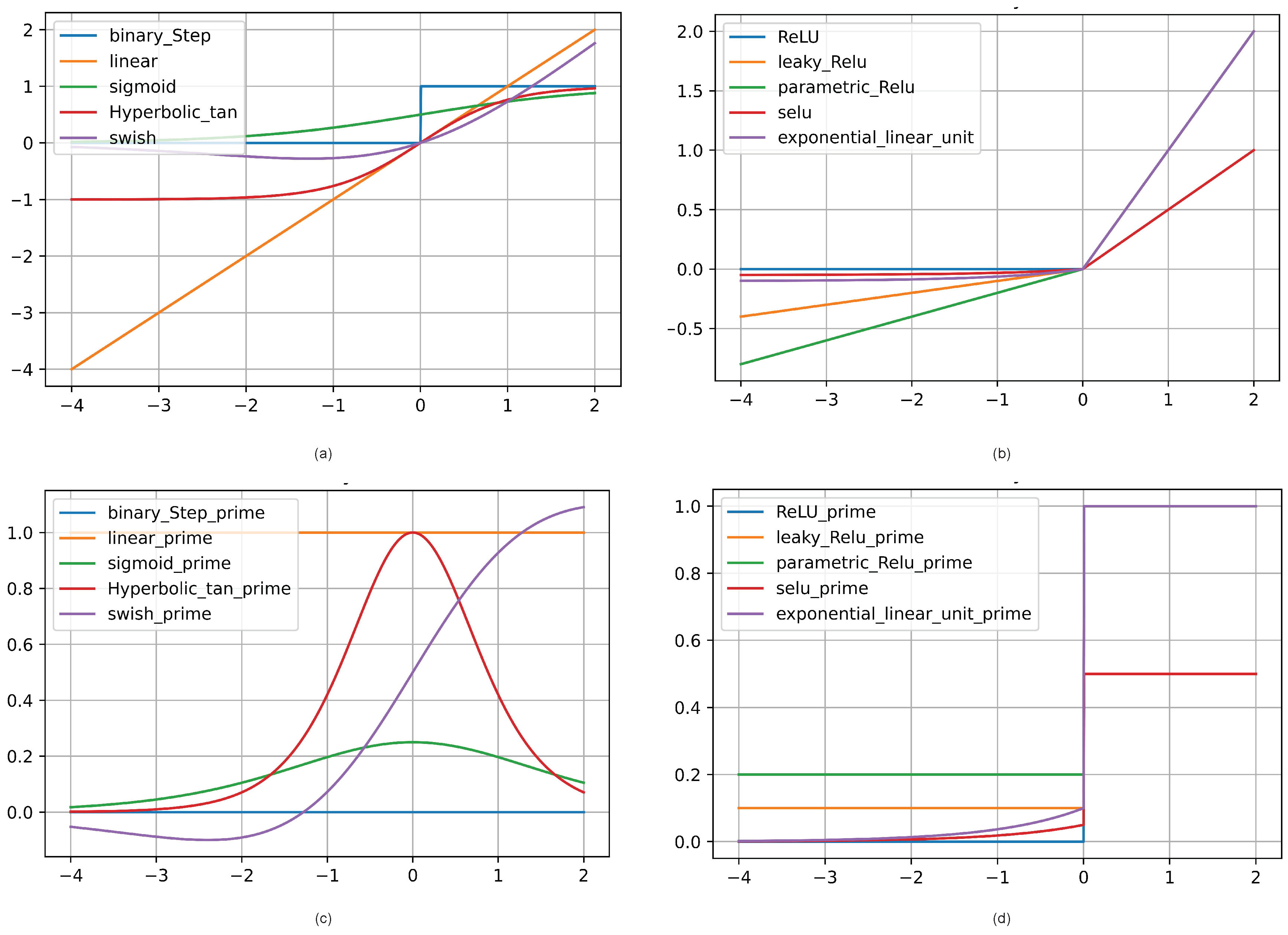
Figure 2.
AIF Activation function drawn in 4 different scales. (a) [-0.2,0.2] scale (b) [-0.5,0.5] scale (c) [-1,1] scale and (d) [-10,10] scale. (we have chosen if else 0.1).
Figure 2.
AIF Activation function drawn in 4 different scales. (a) [-0.2,0.2] scale (b) [-0.5,0.5] scale (c) [-1,1] scale and (d) [-10,10] scale. (we have chosen if else 0.1).
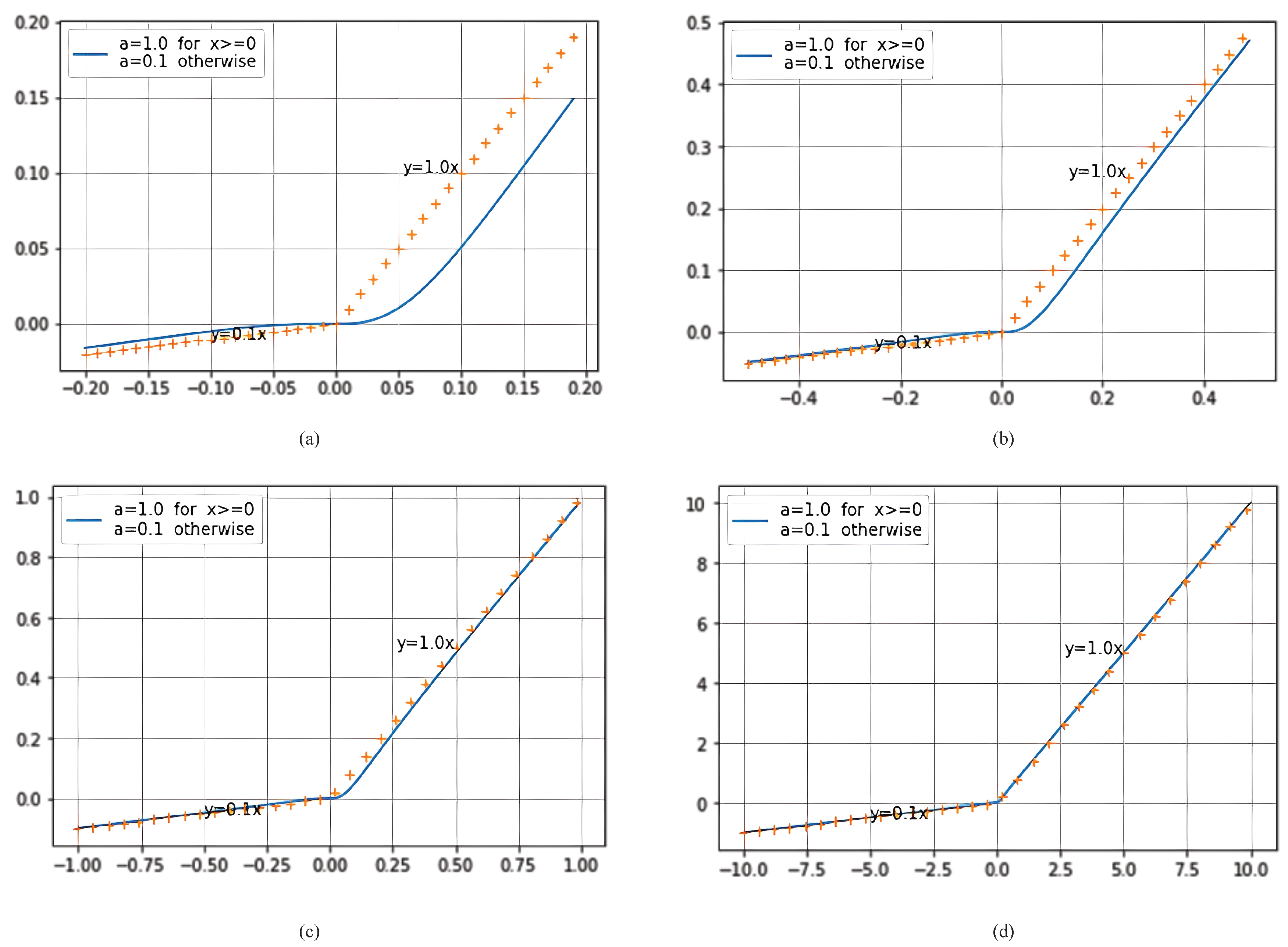
Figure 3.
AIF activation function and its first-order derivative. a: Illustrates AIF diagrams. b: Shows the derivative of AIF.
Figure 3.
AIF activation function and its first-order derivative. a: Illustrates AIF diagrams. b: Shows the derivative of AIF.
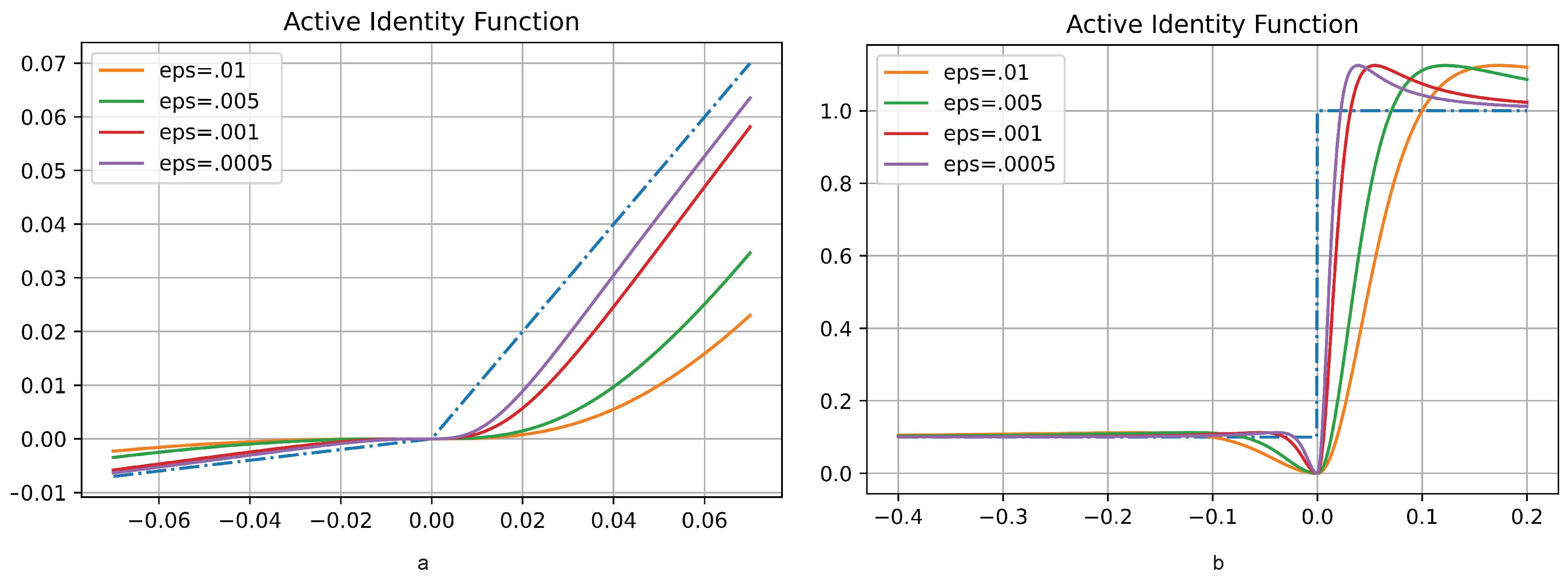
Figure 4.
(a) First and (b) Second derivative of AIF with a=0.1, .
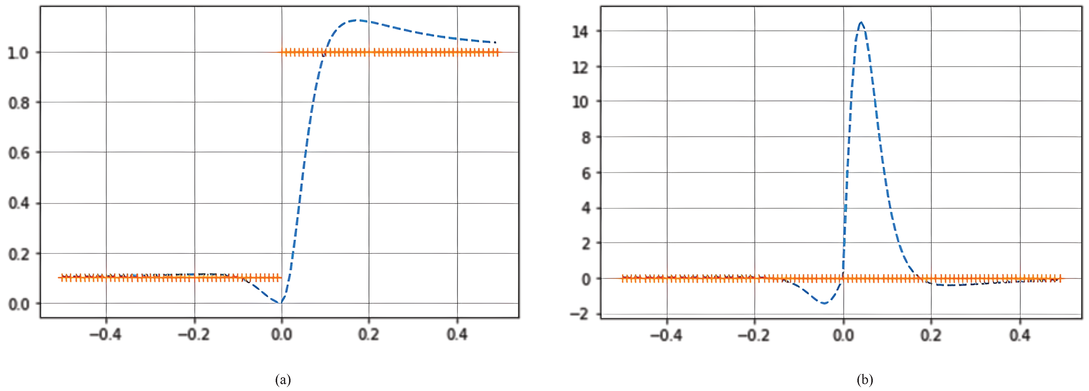
Figure 5.
Evaluation of Caps Net with AIF and SWISH Activation Function. The test and train accuracy of the model is better when we use AIF instead of SWISH.
Figure 5.
Evaluation of Caps Net with AIF and SWISH Activation Function. The test and train accuracy of the model is better when we use AIF instead of SWISH.
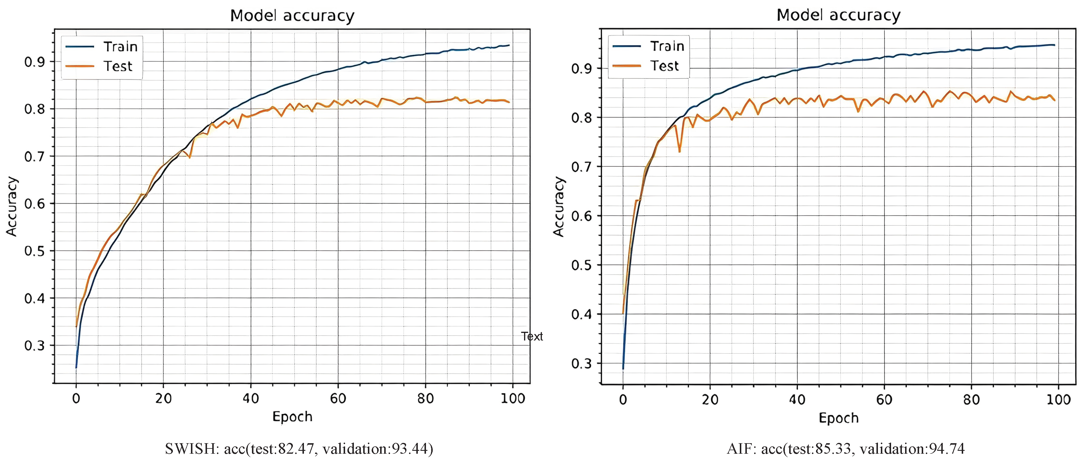
Figure 6.
Net2Net Network Evaluation Chart on Cifar10 Data with AIF and SWISH Activation Function.
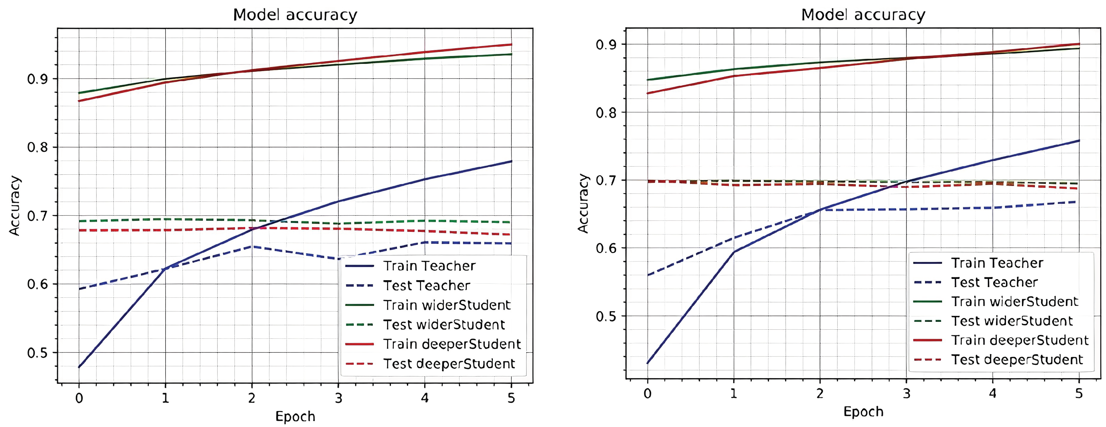
Figure 7.
Net2Net Network Evaluation Chart on MNIST Data with AIF and SWISH Activation Functions. The test accuracy from left to right is based on teacher data, wider student data, and deeper student data.
Figure 7.
Net2Net Network Evaluation Chart on MNIST Data with AIF and SWISH Activation Functions. The test accuracy from left to right is based on teacher data, wider student data, and deeper student data.
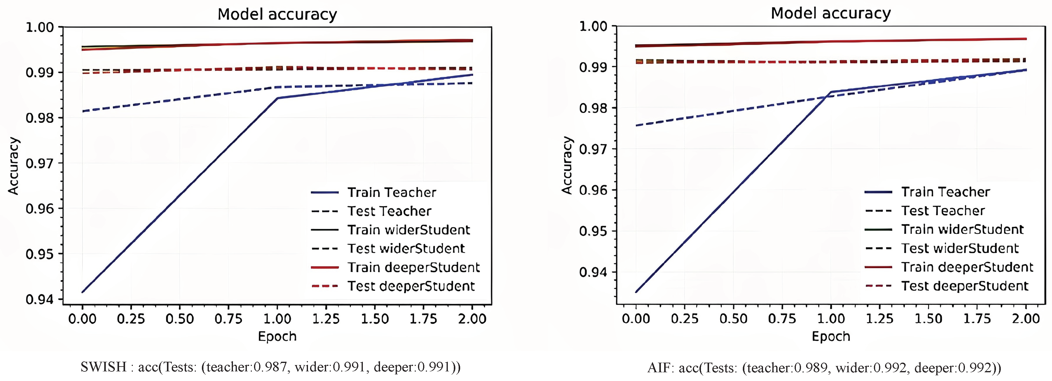
Figure 8.
Compares AIF and SWISH in transfer learning on ImageNet data. AIF reaches its maximum accuracy faster than SWISH (12th vs. 43rd epochs).
Figure 8.
Compares AIF and SWISH in transfer learning on ImageNet data. AIF reaches its maximum accuracy faster than SWISH (12th vs. 43rd epochs).
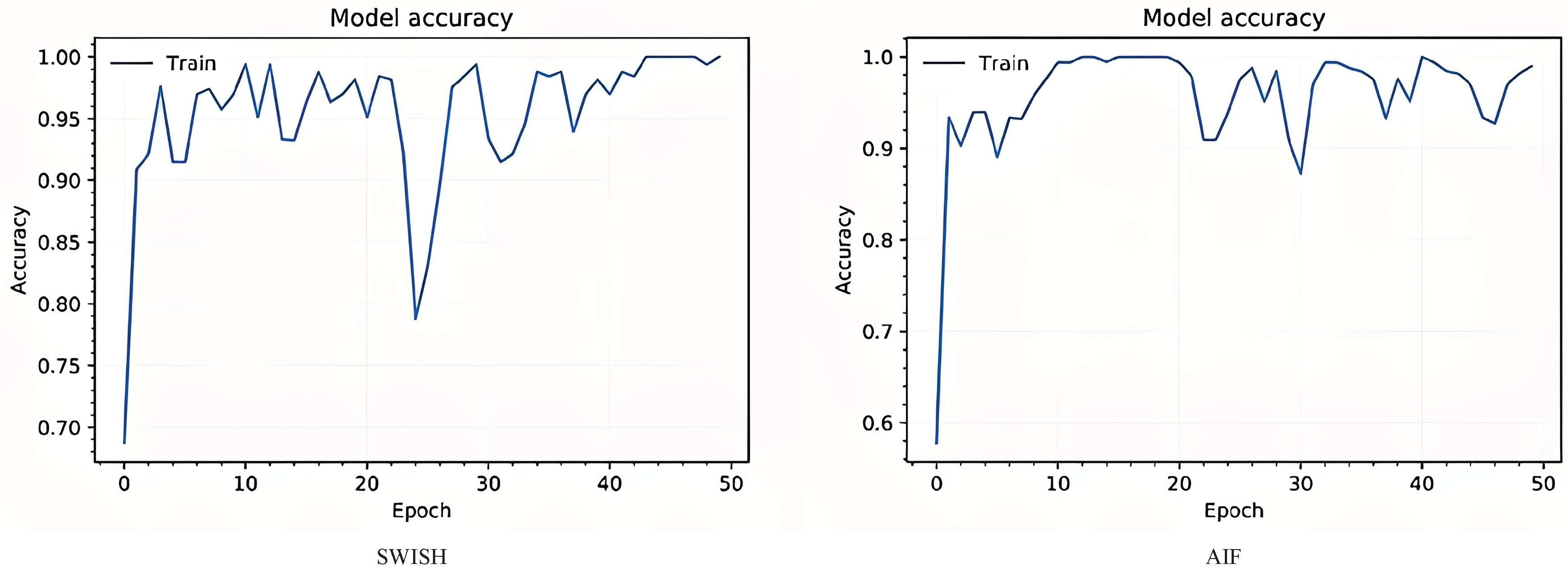
Figure 9.
ResNet20_v1 Network Evaluation Chart with AIF and SWISH Activation Function. From left to right, accuracy, and validation accuracy are given for each activation function.
Figure 9.
ResNet20_v1 Network Evaluation Chart with AIF and SWISH Activation Function. From left to right, accuracy, and validation accuracy are given for each activation function.
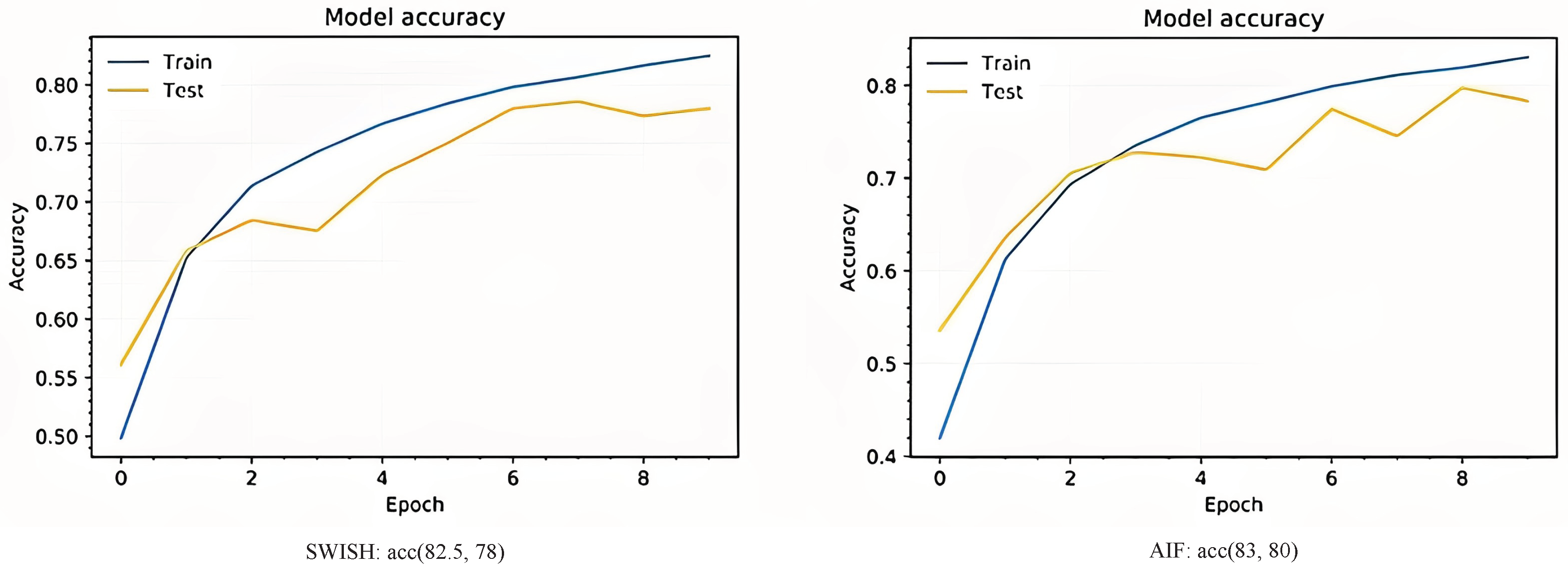
Figure 10.
ResNet20_v1 Network Evaluation Chart with AIF and SWISH Activation Function. From left to right, accuracy, and validation accuracy are given for each activation function.
Figure 10.
ResNet20_v1 Network Evaluation Chart with AIF and SWISH Activation Function. From left to right, accuracy, and validation accuracy are given for each activation function.
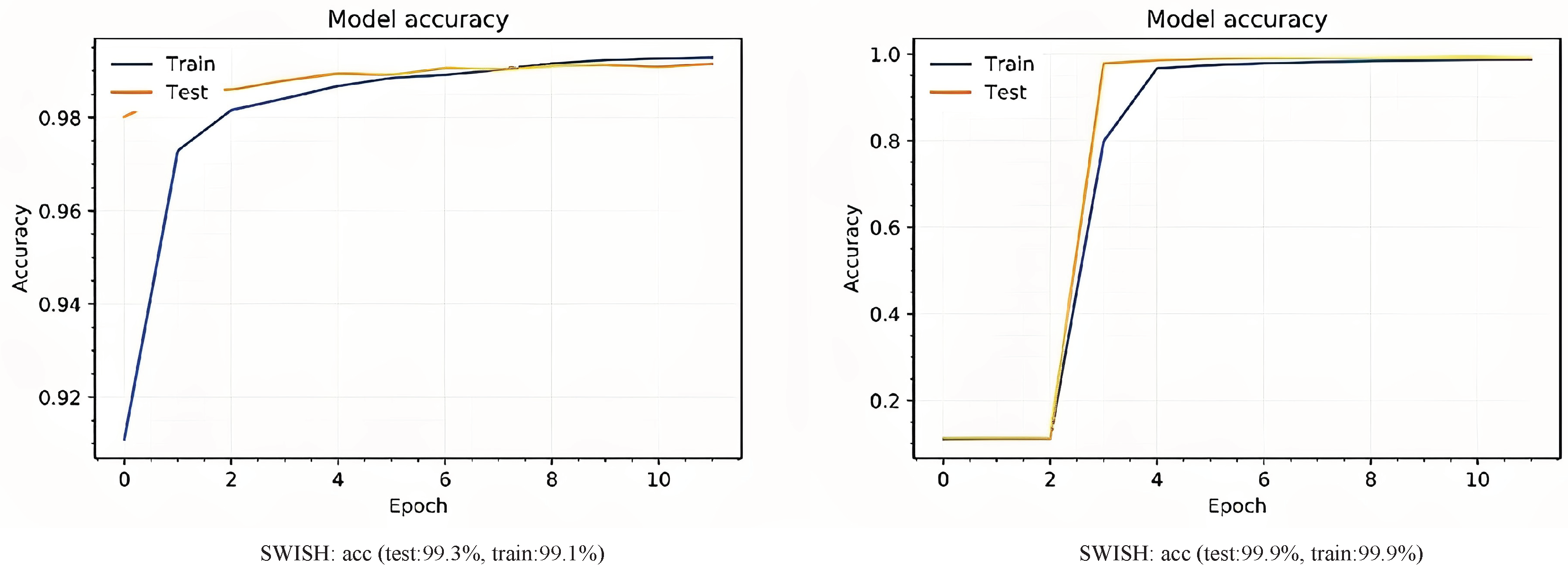
Figure 11.
Activation distribution for SWISH, RELU, and AIF.
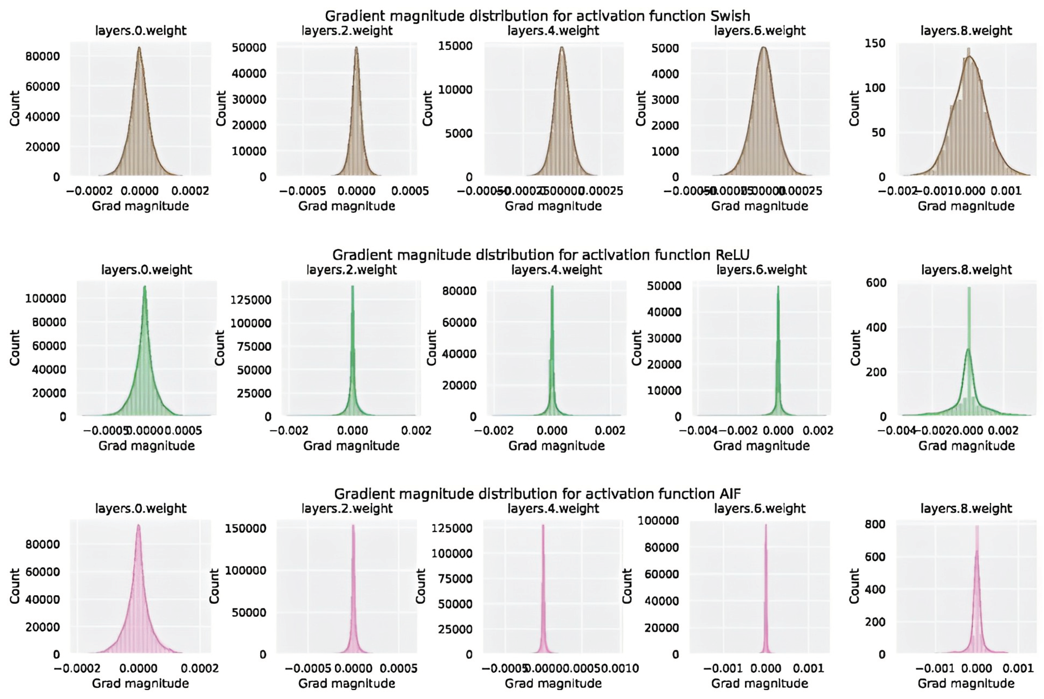

Table 1.
Comparing the AIF to the SWISH activation function.
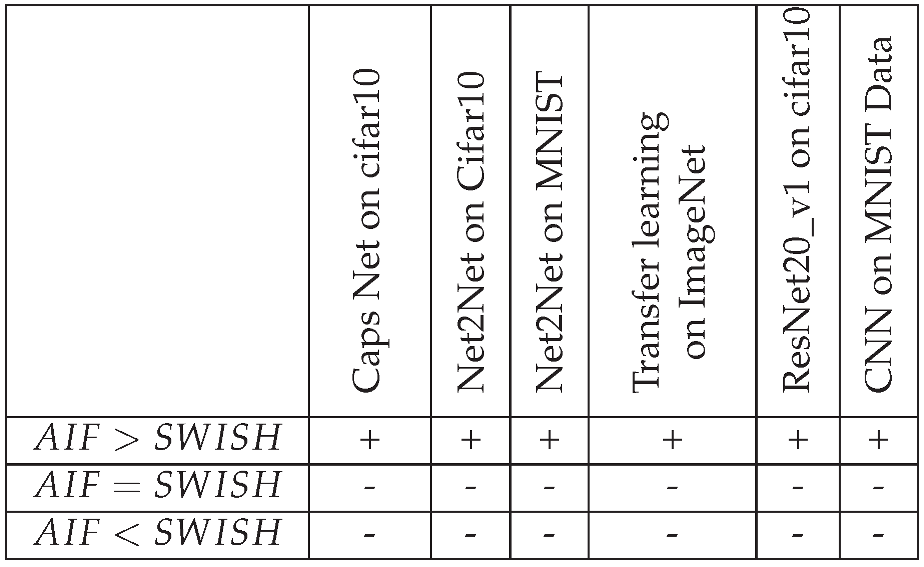 |
Table 2.
Comparison of AIF with some other widely used activation functions.
 |
Disclaimer/Publisher’s Note: The statements, opinions and data contained in all publications are solely those of the individual author(s) and contributor(s) and not of MDPI and/or the editor(s). MDPI and/or the editor(s) disclaim responsibility for any injury to people or property resulting from any ideas, methods, instructions or products referred to in the content. |
© 2023 by the authors. Licensee MDPI, Basel, Switzerland. This article is an open access article distributed under the terms and conditions of the Creative Commons Attribution (CC BY) license (https://creativecommons.org/licenses/by/4.0/).
Copyright: This open access article is published under a Creative Commons CC BY 4.0 license, which permit the free download, distribution, and reuse, provided that the author and preprint are cited in any reuse.


