

Submitted:
07 June 2023
Posted:
09 June 2023
You are already at the latest version
Abstract
In this article, we investigate the applicability of quantum machine learning for classification tasks using two quantum classifiers from the Qiskit Python environment: the Variational Quantum Classifier (VQC) and the Quantum Kernel Estimator (QKE). We evaluate the performance of these classifiers on six widely known and publicly available benchmark datasets and analyze how their performance varies with the number of samples on two artificially generated test classification datasets. As quantum machine learning is based on unitary transformations, this paper explores data structures and application fields that could be particularly suitable for quantum advantages. Hereby, we developed a data set based on concepts from quantum mechanics using the exponential map of a Lie algebra. This dataset will be made publicly available and contributes a novel contribution to the empirical evaluation of quantum supremacy. We further compared the performance of VQC and QKE on six widely applicable datasets to contextualize our results.\\ Our results demonstrate that the VQC and QKE perform better than basic machine learning algorithms such as advanced linear regression models (Ridge and Lasso). They do not match the accuracy and runtime performance of sophisticated modern boosting classifiers like XGBoost, LightGBM, or CatBoost. Therefore, we conclude that while quantum machine learning algorithms have the potential to surpass classical machine learning methods in the future, especially when physical quantum infrastructure becomes widely available, they currently lag behind classical approaches. Our investigations also show that classical machine learning approaches have superior performance classifying datasets based on group structures, compared to quantum approaches that particularly use unitary processes.\\ Furthermore, our findings highlight the significant impact of different quantum simulators, feature maps, and quantum circuits on the performance of the employed quantum estimators. This observation emphasizes the need for researchers to provide detailed explanations of their hyperparameter choices for quantum machine learning algorithms, as this aspect is currently overlooked in many studies within the field.\\ To facilitate further research in this area and ensure the transparency of our study, we have made the complete code available in a linked GitHub repository.
Keywords:
quantum machine learning
; Variational Quantum Circuit
; Quantum Kernel Estimator
; Qiskit
; Ridge
; Lasso
; XGBoost
; LightGBM
; CatBoost
; classification
; quantum computing
; boost classifiers
; neural networks
Quantum computing has recently gained significant attention due to its potential to solve complex computational problems exponentially faster than classical computers [1]. Quantum machine learning (QML) is an emerging field that combines the power of quantum computing with traditional machine learning techniques to solve real-world problems more efficiently [2,3]. Various QML algorithms have been proposed, such as Quantum Kernel Estimator (QKE) [4] and Variational Quantum Classifier (VQC) [5], which have shown promising results in diverse applications, including pattern recognition and classification tasks, [6,7,8].
In this study, we aim to compare QKE (Quantum Kernel Estimator) and VQC (Variational Quantum Circuit) with powerful classical machine learning methods such as XGBoost [9], Ridge [10], Lasso [11], LightGBM [12], CatBoost [13], and MLP (Multi-Layer Perceptron) [14] on six benchmark data sets partially available in the scikit-learn library [15] as well as artificially generated data sets. To ensure a fair comparison on the benchmark data sets, we perform a randomized search to optimize hyperparameters for each algorithm, thereby providing a comprehensive statistical comparison of their performance. Further, we provide the full program code in a GitHub repository [16] to make our results reproducible and boost research that can potentially build on our approach.
Since quantum machines are not readily accessible, we can only compare these algorithms’ performance on simulated quantum circuits. Although this approach does not reveal the full potential of quantum machine learning, it does highlight how the discussed quantum machine learning methods handle different levels of complexity inherent in the data sets. For this reason, we also developed a method to generate artificial data sets based on quantum mechanical concepts to provide a prototype for a particularly well-suited data set for quantum machine learning. This will estimate the possible improvements that quantum machine learning algorithms can offer over classical methods in terms of accuracy and efficiency, considering the computational resources needed to simulate quantum circuits.
In this study, we address and partially answer the following research questions:
- How do QKE and VQC algorithms compare to classical machine learning methods such as XGBoost, Ridge, Lasso, LightGBM, CatBoost, and MLP regarding accuracy and efficiency on simulated quantum circuits?
- To what extent can randomized search make the performance of quantum algorithms comparable to classical approaches?
- What are the limitations and challenges associated with the current state of quantum machine learning, and how can future research address these challenges to unlock the full potential of quantum computing in machine learning applications?
- Do quantum machine learning algorithms outperform regular machine learning algorithms on data sets constrained by the rules of quantum mechanics? Thus, do they provide a quantum advantage for data sets that exhibit strong symmetry properties in terms of adhering to Lie algebras?
The research presented in this article is partially inspired by the work of Zeguendry et al. [17], which offers an excellent review and introduction to quantum machine learning. However, their article does not delve into the tuning of hyperparameters for the quantum machine learning models employed, nor does it provide ideas on creating best-suited data for Quantum Machine Learning classification tasks. We aim to expand the toolbox of quantum machine learning, first by discussing the space of Hyperparameters and second by providing a prototype for generating "quantum data". Further, this analysis will help determine the current state of quantum machine learning performance and whether researchers should employ these algorithms in their studies.
We provide the entire program code of our experiments and all the results in a GitHub repository, ensuring the integrity of our findings, fostering research in this field, and offering a comprehensive code for researchers to test quantum machine learning on their classification problems. Thereby, a key contribution of our research is not only the provision of a single implementation of a quantum machine learning algorithm but also the execution of a randomized search for potential hyperparameters of both classical and quantum machine learning models and a novel approach for generating artificial classification problems based on concepts inherent to Quantum Mechanics, i.e., Lie groups and algebras.
This article is structured as followes:
Section 1 discusses relevant and related work.
In Section 2, we describe, reference, and to some degree, derive all employed techniques. We will not discuss the mathematical details of all employed algorithms here but rather refer the interested reader to the referenced sources.
The following Section 3 describes our performed experiments in detail, followed by the obtained results in Section 4, which also features a discussion of our findings.
Finally we conclude our findings in Section 5.
1. Related Work
Considerable research was conducted in the last years to advance quantum machine learning environments and their application field. This starts in the data encoding process, in which Schuld and Killoran [3]investigated quantum machine learning in feature Hilbert spaces theoretically. They proposed a framework for constructing quantum embeddings of classical data to enable quantum algorithms that learn and classify data in quantum feature spaces.
Further research was conducted on introducing novel architectural frameworks. For such, Mitarai et al. [18] presented a method called quantum circuit learning (QCL), which uses parameterized quantum circuits to approximate classical functions. QCL can be applied to supervised and unsupervised learning tasks, as well as reinforcement learning.
Havlíček et al. [4] introduced a quantum-enhanced feature space approach using variational quantum circuits. This work demonstrated that quantum computers can effectively process classical data with quantum kernel methods, offering the potential for exponential speedup in certain applications.
Furthermore, Farhi and Neven [5] explored the use of quantum neural networks for classification tasks on near-term quantum processors. They showed that quantum neural networks can achieve good classification performance with shallow circuits, making them suitable for noisy intermediate-scale quantum (NISQ) devices.
Other research focused on the advancement of applying quantum fundamentals on classical machine learning applications. Hereby, Rebentrost et al. [19] introduced the concept of a quantum support vector machine for big data classification. They showed that the quantum version of the algorithm can offer exponential speedup compared to its classical counterpart, specifically in the kernel evaluation stage.
To advance the application field of Quantum Machine Learning, Liu and Rebentrost [20] proposed a quantum machine learning approach for quantum anomaly detection. They demonstrated that their method can efficiently solve classification problems, even when the data has a high degree of entanglement.
In this regard, it is worth mentioning the work of Broughton et al. [21] introduced TensorFlow Quantum, an open-source library for the rapid prototyping of hybrid quantum-classical models for classical or quantum data. They demonstrated various applications of TensorFlow Quantum, including supervised learning for quantum classification, quantum control, simulating noisy quantum circuits, and quantum approximate optimization. Moreover, they showcased how TensorFlow Quantum can be applied to advanced quantum learning tasks such as meta-learning, layerwise learning, Hamiltonian learning, sampling thermal states, variational quantum eigensolvers, classification of quantum phase transitions, generative adversarial networks, and reinforcement learning.
In the review paper by Zeguendry et al. [17], the authors present a comprehensive overview of quantum machine learning (QML) from the perspective of conventional machine learning techniques. The paper starts by exploring the background of quantum computing, its architecture, and an introduction to quantum algorithms. It then delves into several fundamental algorithms for QML, which form the basis of more complex QML algorithms and can potentially offer performance improvements over classical machine learning algorithms. In the study, the authors implement three machine learning algorithms: Quanvolutional Neural Networks, Quantum Support Vector Machines, and Variational Quantum Classifier (VQC). They compare the performance of these quantum algorithms with their classical counterparts on various datasets. Specifically, they implement Quanvolutional Neural Networks on a quantum computer to recognize handwritten digits and compare its performance to Convolutional Neural Networks, stating the performance improvements by quantum machine learning.
Despite these advancements, it is important to note that some of the discussed papers may not have used randomized search CV from scikit-learn to optimize the classical machine learning algorithms, thereby, overstating the significance of quantum supremacy. Nevertheless, the above-mentioned works present a comprehensive overview of the state of the art in quantum machine learning for classification, highlighting the potential benefits of using quantum algorithms in various forms and applications.
2. Methodology
This section presents our methodology for comparing the performance of classical and quantum machine learning techniques for classification tasks. Our approach is designed to provide a blueprint for future experiments in this area of research. We employ the Scikit-learn library, focusing on the inbuilt functions to select a good set of hyperparameters, i.e., RandomizedSearchCV to compare classical and quantum machine learning models. We also utilize the Qiskit library to incorporate quantum machine learning techniques into our experiments, [22]. The selected data sets for our study include both real-world and synthetic data, enabling a comprehensive evaluation of the classifiers’ performance.
2.1. Supervised Machine Learning
Supervised Machine Learning is a subfield of artificial intelligence that focuses on developing algorithms and models to learn patterns and make decisions or predictions based on data [23,24]. The main goal of supervised learning is to predict labels or outputs of new, unseen data given a set of known input-output pairs (training data). This section briefly introduces several classical machine learning techniques used for classification tasks, specifically in the context of supervised learning. These techniques serve as a baseline to evaluate the applicability of quantum machine learning approaches, which are the focus of this paper. Further, we will then introduce the employed quantum machine learning algorithms.
One of the essential aspects of supervised machine learning is the ability to predict/classify data. The models are trained using a labeled dataset, and then the performance of the models is evaluated based on their accuracy in predicting the labels of previously unseen test samples [25]. This evaluation is crucial to estimate the model’s ability to generalize the learned information when making predictions on new, real-world data.
Various techniques, such as cross-validation and train-test splits, are often used to obtain reliable performance estimates of the models [26]. By comparing the performance of different models, researchers and practitioners can determine which model or algorithm is better suited for a specific problem domain.
2.2. Classical Supervised Machine Learning Techniques
The following list describes the employed algorithms that serve as a baseline for the afterwards described and later tested quantum machine learning algorithms.
-
Lasso and Ridge Regression/Classification: Lasso (Least Absolute Shrinkage and Selection Operator) and Ridge Regression are linear regression techniques that incorporate regularization to prevent overfitting and improve model generalization [10,27]. Lasso uses L1 regularization, which tends to produce sparse solutions, while Ridge Regression uses L2 regularization, which prevents coefficients from becoming too large.Both of these regression algorithms can also be used for classification tasks.
- Multilayer Perceptron (MLP): MLP is a type of feedforward artificial neural network with multiple layers of neurons, including input, hidden, and output layers [14]. MLPs are capable of modeling complex non-linear relationships and can be trained using backpropagation.
- Support Vector Machines (SVM): SVMs are supervised learning models used for classification and regression tasks [28]. They work by finding the optimal hyperplane that separates the data into different classes, maximizing the margin between the classes.
- Gradient Boosting Machines: Gradient boosting machines are an ensemble learning method that builds a series of weak learners, typically decision trees, to form a strong learner [29]. The weak learners are combined by iteratively adding them to the model while minimizing a loss function. Notable gradient boosting machines for classification tasks include XGBoost [9], CatBoost [13], and LightGBM [12]. These three algorithms have introduced various improvements and optimizations to the original gradient boosting framework, such as efficient tree learning algorithms, handling categorical features, and reducing memory usage.
2.3. Quantum Machine Learning
Quantum machine learning is an emerging interdisciplinary field that leverages the principles of quantum mechanics and quantum computing to improve or develop novel algorithms for machine learning tasks [2]. This section introduces two key quantum machine learning techniques, Variational Quantum Classifier (VQC) and Quantum Kernel Estimator (QKE), and discusses their connections to classical machine learning techniques. Additionally, we briefly introduce Qiskit Machine Learning, a Python package developed by IBM for implementing quantum machine learning algorithms. Also, we want to mention the work done by [17] for a review of quantum machine learning algorithms and a more detailed discussion of the employed algorithms.
2.3.1. Variational Quantum Classifier (VQC):
VQC is a hybrid quantum-classical algorithm that can be viewed as a quantum analog of classical neural networks, specifically the Multilayer Perceptron (MLP) [4]. VQC employs a parametrized quantum circuit, which is trained using classical optimization techniques to find the optimal parameters for classification tasks. The learned quantum circuit can then be used to classify new data points.
Figure 1 illustrates the schematic depiction of the Variational Quantum Circuit (VQC), which involves preprocessing the data, encoding it onto qubits using a feature map, processing it through a variational quantum circuit (Ansatz), measuring the final qubit states, and optimizing the circuit parameters , Thus the main building blocks of the VQC are:
- Preprocessing: The data is prepared and preprocessed before being encoded onto qubits.
- Feature Map Encoding (yellow in the figure): The preprocessed data is encoded onto qubits using a feature map.
- Variational Quantum Circuit (Ansatz) (steel-blue in the figure): The encoded data undergoes processing through the variational quantum circuit, also known as the Ansatz, which consists of a series of quantum gates and operations.
- Measurement (orange in the figure): The final state of the qubits is measured, providing probabilities for the different quantum states.
- Parameter Optimization: The variational quantum circuit is optimized by adjusting the parameters , such as the rotations of specific quantum gates, to improve the outcome/classification.
2.3.2. Quantum Kernel Estimator (QKE):
QKE is a technique that leverages the quantum computation of kernel functions to enhance the performance of classical kernel methods, such as Support Vector Machines (SVM) [30].By computing the kernel matrix using quantum circuits, QKE can capture complex data relationships that may be challenging for classical kernel methods to exploit.
The main building blocks for the employed QKE, which are depicted in Figure 2 are:
- Data Preprocessing: The input data is preprocessed, which may include tasks such as data cleaning, feature scaling, or feature extraction. This step ensures that the data is in an appropriate format for the following quantum feature maps.
- Feature Map Encoding (yellow in the figure): The preprocessed data is encoded onto qubits using a feature map.
- Kernel Computation (steel-blue in the figure): Instead of directly computing the kernel matrix from the original data, a kernel function is precomputed using the quantum computing capabilities, meaning that the inner product of two quantum states is estimated on a quantum simulator/circuit. This kernel function captures the similarity between pairs of data points in a high-dimensional feature space.
- SVM Training: The precomputed kernel function is then used as input to the SVM algorithm for model training. The SVM aims to find an optimal hyperplane that separates the data points into different classes with the maximum margin.
Here we need to mention that in the documentation of qiskit-machine-learning, the developers provided a full QKE implementation without the need to use, e.g., scikit-learn’s SVM-implementation. However, as of the writing of this article, this estimator is no longer available in qiskit-machine-learning. Thus, one needs to use a support vector machine implementation from other sources after precomputing the kernel on a quantum simulator.
2.3.3. Qiskit Machine Learning
Qiskit Machine Learning is an open-source Python package developed by IBM for implementing quantum machine learning algorithms [22]. This package enables researchers and practitioners to develop and test quantum machine learning algorithms, including VQC and QKE, using IBM’s quantum computing platform. It provides tools for building and simulating quantum circuits, as well as interfaces to classical optimization and machine learning libraries.
Thus we used this environment and the corresponding Quantum Simulators described in Appendix A for our experiments.
2.4. Accuracy Score for Classification
The accuracy score is a standard metric used to evaluate the performance of classification algorithms. We employed the accuracy score to evaluate all presented experiments. It is defined as the ratio of correct predictions to the total number of predictions. The formula for the accuracy score is defined as follows:
In Scikit-learn, the accuracy score can be computed using the accuracy_score function from the `sklearn.metrics` module [15].
For more information on the accuracy score and its interpretation, refer to the Scikit-learn documentation [15].
2.5. Data Sets
In this study, we used six classification data sets from various sources. Two data sets are part of the Scikit-learn library, while the remaining four are obtained/fetched from OpenML. The data sets are described below:
- Iris Data Set: A widely known data set consisting of 150 samples of iris flowers, each with four features (sepal length, sepal width, petal length, and petal width) and one of three species labels (Iris Setosa, Iris Versicolor, or Iris Virginica). This data set is included in the Scikit-learn library [15].
- Wine Data Set: A popular data set for wine classification, which consists of 178 samples of wine, each with 13 features (such as alcohol content, color intensity, and hue) and one of three class labels (class 1, class 2, or class 3). This data set is also available in the Scikit-learn library [15].
- Indian Liver Patient Dataset (LPD): This data set contains 583 records, with 416 liver patient records and 167 non-liver patient records [31]. The data set includes ten variables: age, gender, total bilirubin, direct bilirubin, total proteins, albumin, A/G ratio, SGPT, SGOT, and Alkphos. The primary task is to classify patients into liver or non-liver patient groups.
- Breast Cancer Coimbra Dataset: This data set consists of 10 quantitative predictors and a binary dependent variable, indicating the presence or absence of breast cancer [32,33]. The predictors are anthropometric data and parameters obtainable from routine blood analysis. Accurate prediction models based on these predictors can potentially serve as a biomarker for breast cancer.
- Teaching Assistant Evaluation Dataset: This data set includes 151 instances of teaching assistant (TA) assignments from the Statistics Department at the University of Wisconsin-Madison, with evaluations of their teaching performance over three regular semesters and two summer semesters [34,35]. The class variable is divided into three roughly equal-sized categories ("low", "medium", and "high"). There are six attributes, including whether the TA is a native English speaker, the course instructor, the course, the semester type (summer or regular), and the class size.
- Impedance Spectrum of Breast Tissue Dataset: This data set contains impedance measurements of freshly excised breast tissue at the following frequencies: 15.625, 31.25, 62.5, 125, 250, 500, and 1000 KHz [36,37]. The primary task is to predict the classification of either the original six classes or four classes by merging the fibro-adenoma, mastopathy, and glandular classes whose discrimination is not crucial.
These data sets were selected for their diverse domains and varied classification tasks, providing a robust testing ground for the quantum classifiers we employed in our experiments.
Further, we used artificially generated data sets to control the number of samples, etc.. Here scikit-learn provides a valuable function called make_classification to generate synthetic classification datasets. This function creates a random n-class classification problem, initially creating clusters of points normally distributed about vertices of an n-informative-dimensional hypercube, and assigns an equal number of clusters to each class [15]. It introduces interdependence between features and adds further noise to the data. The generated data is highly customizable, with options for specifying the number of samples, features, informative features, redundant features, repeated features, classes, clusters per class, and more. For more details on the make_classification function and its parameters, refer to the Scikit-learn documentation available on scikit-learn.org.
2.5.1. Data Obtained from Lie-Algebras
We construct another artificial data set final data set for our final evaluation; however, this time, we do this by using tools from the theory of Lie groups. The reason for employing these concepts is that we want to produce data that resembles the complexity inherent to the Qubit-Vectorspace of quantum machine learning and, further, is generated by applying transformations on vectors that are similar to the manipulations present in Quantum Machin Learning algorithms, e.g., for the VQC, rotations of/around the Bloch-sphere. Thus we overall aim to provide random data for a classification task to show a case where the authors assume Quantum Machine Learning algorithms can, because of their inherent structure, outperform classical machine learning algorithms and thus provide a prototype on the type of data specifically tailored to address the inherent structure of quantum machine learning. The theoretical foundations of this section are obtained from [38], and thus the interested reader is referred to this book for a profound introduction to Lie groups.
To further explain the employed ideas, we start by introducing the concept of a Lie group G and the corresponding Lie-algebra .
A Lie group is a mathematical structure that captures the essence of continuous symmetry. Named after the Norwegian mathematician Sophus Lie, Lie groups are ubiquitous in many areas of mathematics and physics, including the study of differential equations, geometry, and quantum mechanics.
A Lie group is a set G that has the structure of both a smooth manifold and a group in such a way that the group operations (multiplication and inversion) are smooth. That is, a Lie group is a group that is also a differentiable manifold, such that the group operations are compatible with the smooth structure.
Meaning that a Lie group is a set G equipped with a group structure (i.e., a binary operation , that is associative, an identity element , and an inversion operation , ) and a smooth manifold structure such that the following conditions are satisfied:
- The multiplication map defined by is smooth.
- The inversion map defined by is smooth.
A Lie algebra is associated with each Lie group, a vector space equipped with a binary operation called the Lie bracket. The Lie algebra captures the local structure of the Lie group near the identity element, meaning that the Lie algebra of a Lie group G is the tangent space at the identity, denoted , equipped with the Lie bracket operation. The Lie bracket is defined in terms of the group operation and the differential.
There is a map from the Lie algebra to the Lie group called the exponential map, denoted . The exponential map provides a way to generate new group elements from elements of the Lie algebra. In particular, given an element X of the Lie algebra, is a group element close to the identity if X is ’small’. We will exploit this concept to generate random data associated with a specific group:
We start with a set of Generators contained within the Lie-algebra g of a Lie group G, where , i.e., the dimension of the Lie-algebra. We can then create elements by employing
We used the condition for our -values without loss of generality due to the periodicity of the exponential function. To generate our random data, we randomly choose our and create an element of our group. We then apply this element to a corresponding base vector of our vector space.
Specifically, in our example, we use the Lie-group SU(2). The special unitary group of degree 2, denoted as SU(2), is a Lie group of 2x2 unitary matrices with determinant 1.
The corresponding Lie algebra, , consists of 2x2 Hermitian traceless matrices, i.e. the Pauli matrices:
The commutation relations of the Pauli matrices form the structure of the Lie algebra:
where denotes the commutator, and is the Levi-Civita symbol.
To generate a classification data set from this algebra, we use the following procedure:
- Find a set of random parameters
- We then create an element U of SU(2) using these these randomly set parameters:
- Next we take one of the basevectors from , denoted as to create a new complex vector using the previously obtained matrix U such that: .
- This vector is then separated into four features such that:where and denotes the individual components of the vector .
- Finally we assign a class label C to this collection of Features such that:and collect the features and the class label into one sample . We repeat this process times, starting with 1., where is the number of samples that we want for our data set.
Note that this approach can be extended to arbitrary Lie groups, given that one can construct or obtain a Lie group’s generators.
3. Experimental Design
In this section, we describe our experimental design, which aims to provide a fair and comprehensive comparison of the performance of classical machine learning (ML) and quantum machine learning (QML) techniques, as discussed in Section 2.2 and Section 2.3. Our experiments involve two main components: Firstly, assessing the algorithms’ performance on artificially generated data sets with varying parametrizations, and secondly, evaluating the algorithms’ performance on benchmark data sets using randomized search to optimize hyperparameters, ensuring a fair comparison. By carefully selecting our experimental setup, we avoid the issue of "cherry-picking" only a favorable subset of results, a common problem in machine learning leading to heavily-biased conclusions.
3.1. Artificially Generated Sci-Kit Data Sets
To generate the synthetic classification dataset, we utilized scikit-learn’s
make_classification function. We employed two features and two classes while varying the number of samples to obtain a performance curve illustrating how the chosen algorithms’ performance changes depending on the sample size.
We partitioned each dataset such that 20% of the original data was reserved as a test set to evaluate the trained algorithm, producing the accuracy score used for our assessment. Further, each data set was normalized such that all features are within the unit interval .
As a baseline, we employed the seven classical machine learning algorithms described in Section 2.2, namely Lasso, Ridge, MLP, SVM, XGBoost, LightGBM, and CatBoost. We used two different parameterizations for the classical machine learning algorithms for our comparisons. Firstly, we applied the out-of-the-box implementation without any hyperparameter optimization. Secondly, we used an optimized version of each algorithm found through scikit-learn’s RandomizedSearchCV by testing 20 different models.
We then examined 20 distinct parameter configurations, each for the VQC and QKE classifiers, randomly selected from a predefined parameter distribution. Appendix A discusses the parameter grids for all utilized algorithms and all experiments.
3.2. Artificially Generated SU(2) Data Sets
For our synthetic classification dataset, we used the concepts previously discussed in Section 2.5.1. We employed two complex features, i.e. resulting in four continuous real features, and two classes while varying the number of samples to obtain a performance curve illustrating how the chosen algorithms’ performance changes depending on the sample size.
We partitioned each dataset such that 20% of the original data was reserved as a test set to evaluate the trained algorithm, producing the accuracy score used for our assessment. Further, each data set was normalized such that all features are within the unit interval .
As a baseline, we employed the seven classical machine learning algorithms described in Section 2.2, namely Lasso, Ridge, MLP, SVM, XGBoost, LightGBM, and CatBoost. We used two different parameterizations for the classical machine learning algorithms for our comparisons. Firstly, we applied the out-of-the-box implementation without any hyperparameter optimization. Secondly, we used an optimized version of each algorithm found through scikit-learn’s RandomizedSearchCV by testing 20 different models.
We then examined 20 distinct parameter configurations, each for the VQC and QKE classifiers, randomly selected from a predefined parameter distribution. Appendix A discusses the parameter grids for all utilized algorithms and all experiments.
3.3. Benchmark Data Sets and Hyperparameter Optimization
Our last experiment was to test the two employed quantum machine learning algorithms against the classical machine learning algorithms on six benchmark data sets (Section 2.5). For this reason, we employed scikit-learn’s RandomizedSearchCV to test 20 randomly parameterized models for each algorithm to report the best of these tests. Again we used a train-test-split to keep 20% of the original data to test the trained algorithm. Further, each data set was normalized such that all features are within the unit interval .
4. Results
In this section, we present the results of our experiments, comparing the performance of classical machine learning (ML) and quantum machine learning (QML) techniques on both artificially generated data sets and benchmark data sets (Section 2.5). By analyzing the results, we aim to draw meaningful insights into the strengths and weaknesses of each approach and provide a blueprint for future studies in the area.
4.1. Performance on Artificially Generated Sci-Kit Data Sets
In this section, we compare the performance of quantum machine learning (QML) algorithms and classical machine learning (ML) algorithms on artificially generated classification datasets. The comprehensive experimental setup can be found in Section 3.1.
Regarding accuracy and runtime, our findings are presented in Table 1 and Table 2 and Figure 3, Figure 4, and Figure 5. While QML algorithms perform reasonably well, we observe that they are not a match for properly trained and/or sophisticated state-of-the-art classifiers. Even out-of-the-box implementations of state-of-the-art ML algorithms outperform QML algorithms on these artificially generated classification datasets.
The accuracy of the algorithms varies depending on the dataset size, with larger datasets posing more challenges. CatBoost performed best in our experiments, both out-of-the-box and when optimized in terms of high accuracy over all experiments. The Quantum Kernel Estimator (QKE) is the third-best algorithm overall in terms of accuracy, though it outperforms CatBoost regarding the runtime for CatBoost’s optimized version. XGBoost and Support Vector Classification (SVC) follow closely, with competitive performances in terms of accuracy. However, Variational Quantum Circuit (VQC) struggles to achieve high accuracy compared to sophisticated boosting classifiers or support vector machines.
Other algorithms, such as Multi-Layer Perceptron (MLP), Ridge regression, Lasso regression, and LightGBM, exhibit varying performances depending on data set size and optimization. Despite some reasonable results from QKE, we conclude that classical ML algorithms, particularly sophisticated boosting classifiers, should be chosen to tackle similar problems due to their ease of implementation, better runtime, and overall superior performance.
In summary, while QML algorithms have shown some promise, they cannot yet compete with state-of-the-art classical ML algorithms on artificially generated classification datasets in terms of accuracy and runtime.
4.2. Performance on Artificially Generated SU2 Data Sets
In this section, we compare the performance of quantum machine learning (QML) algorithms and classical machine learning (ML) algorithms on artificially generated classification datasets based on Lie group structures. The detailled experimental setup can be found in Section 3.2.
Regarding accuracy and runtime, our findings are presented in Table 3 and Table 4 and Figure 6, Figure 7, and Figure 8. While QML algorithms perform reasonably well, we observe that they are not a match for properly trained and/or sophisticated state-of-the-art classifiers. Even out-of-the-box implementations of state-of-the-art ML algorithms outperform QML algorithms even on artificially generated classification datasets that are particularly suited for QML.
The accuracy of the algorithms varies depending on the dataset size, with larger datasets providing increased accuracy for most algorithms. CatBoost performed best in our experiments, both out-of-the-box and when optimized in terms of high accuracy over all experiments. The Quantum Kernel Estimator (QKE) is the fourth-best algorithm overall in terms of accuracy. However, we observe that, on average, CatBoost performs best over all experiments out of the box, but is outperformed by the best QKE implementation for 1000 and 1500 data points. Thus we conclude that Quantum Kernel estimators can capture the complexity of this -generated data set, but overall, one is better off with an out-of-the-box CatBoost implementation. Meaning that we do not observe a quantum advantage for this type of data but rather that the employed quantum kernel estimator behaves similarly to classical machine learning algorithms, i.e., it exhibits reasonable performance but does not perform best for all data sets, even the ones created by exploiting quantum symmetry properties.
Other algorithms, such as Multi-Layer Perceptron (MLP), Ridge regression, Lasso regression, and LightGBM, exhibit varying performances depending on data set size and optimization. Despite some reasonable results from QKE, we conclude that classical ML algorithms, particularly sophisticated boosting classifiers, should be chosen to tackle similar problems due to their ease of implementation, better runtime, and overall superior performance.
In summary, while QML algorithms have shown some promise, they cannot yet compete with state-of-the-art classical ML algorithms even on these -data sets, where the authors intended to provide evidence for the quantum advantage for data sets generated from symmetry properties inherent to quantum mechanics.
4.3. Results on Benchmark Data Sets
In this section, we discuss the performance of quantum machine learning (QML) and classical machine learning (ML) algorithms on six benchmark datasets described in Section 2.5. We include results for the quantum classifiers detailed in Section 2.3 and the classical machine learning classifiers discussed in Section 2.2. The scores/accuracies were obtained using Randomized Search cross-validation from Scikit-learn with 20 models and 5-fold cross-validation. Further, everything was calculated on our local machine using an Intel(R) Core(TM) i7-4770 CPU 3.40GHz and 16GB RAM.
Our results, shown in Table 5, display the best 5-fold cross-validation scores (upper table) and the scores of the best model evaluated on an unseen test subset of the original data (lower table), which makes up 20% of the original data. We observe varying performances of the algorithms on these benchmark datasets.
Notably, Variational Quantum Circuit (VQC) and Quantum Kernel Estimator (QKE) classifiers show competitive performance on several datasets but do not consistently outperform classical ML algorithms. In particular, QKE achieves a perfect score on the Iris dataset, but its performance varies across the other datasets.
Classical ML algorithms, such as Multi-Layer Perceptron (MLP), Support Vector Machines (SVM), XGBoost, LightGBM, and CatBoost, exhibit strong performance across all data sets, with some algorithms achieving perfect scores on multiple data sets. CatBoost consistently performs well, ranking as the top-performing algorithm on three of the six datasets. Ridge and Lasso regression show high accuracy on Iris and Wine datasets but perform poorly on the others.
When comparing the runtimes of the experiments, as presented in Table 6, it becomes evident that QML algorithms take substantially longer to execute than their classical counterparts. For instance, the VQC and QKE classifiers take hours to days to complete on various datasets, whereas classical ML algorithms such as Ridge, Lasso, MLP, SVM, XGBoost, LightGBM, and CatBoost typically take seconds to minutes.
This significant difference in runtimes could be attributed to the inherent complexity and resource requirements of QML algorithms, which generally demand specialized quantum hardware and simulators. On the other hand, classical ML algorithms are optimized for execution on conventional hardware, making them more efficient and faster to run.
In conclusion, while QML algorithms like VQC and QKE demonstrate potential in achieving competitive performance on certain datasets, their relatively longer runtimes and less consistent performance across the benchmark datasets may limit their practical applicability compared to classical ML algorithms. Classical ML algorithms such as CatBoost, XGBoost, and LightGBM continue to offer superior and more consistent performance with faster execution times, solidifying their place as reliable and powerful tools for classification tasks.
4.4. Comparison and Discussion
In this study, we have compared the performance of quantum machine learning (QML) and classical machine learning (ML) algorithms on six benchmark datasets and two types of artificially generated classification datasets. We included results for quantum classifiers, such as Variational Quantum Circuit (VQC) and Quantum Kernel Estimator (QKE), and classical machine learning classifiers like CatBoost, XGBoost, and LightGBM. Our experiments showed that while QML algorithms demonstrate potential in achieving competitive performance on certain datasets, they do not consistently outperform classical ML algorithms. Additionally, their longer runtimes and less consistent performance across the benchmark data sets may limit their practical applicability compared to classical ML algorithms, which continue to offer superior and more consistent performance with faster execution times. Further, we constructed artificial data sets with the structure and rulings of Quantum Mechanics in mind. I.e., we used symmetry properties and unitary transformations to generate a classification data set from -matrices in order to demonstrate an advantage of quantum machine learning algorithms to tackle problems with an inherent structure relatable to that of quantum circuits and Quantum Mechanics overall. However, also for these data sets, the employed quantum machine learning algorithms performed reasonably but did not outperform sophisticated boost classifiers. Thus we cannot conclude a quantum advantage for these data sets.
It is essential to highlight that the QML algorithms’ performance in our experiments was based on simulated quantum infrastructures. This is a significant limitation to consider, as the specific constraints and characteristics of the simulated hardware may influence the performance of these algorithms. Further, given the rapid advancement of quantum technologies and hardware, this constraint might be obsolete in the near future.
The impact of quantum simulators, feature maps, and quantum circuits on the performance of quantum estimators stems from the fact that these components play crucial roles in shaping the behavior and capabilities of quantum machine learning algorithms. Quantum simulators, which emulate quantum systems on classical computers, introduce various levels of approximation and noise, leading to deviations from ideal quantum behavior. Different simulators may employ distinct algorithms and techniques, resulting in variations in performance.
Feature maps, responsible for encoding classical data into quantum states, determine how effectively the quantum system can capture and process information. The choice of feature map can greatly influence the ability of quantum algorithms to extract meaningful features and represent the data in a quantum-mechanical space.
Similarly, quantum circuits, composed of quantum gates and operations, define the computational steps performed on the encoded data. Different circuit designs and configurations can affect the expressiveness and depth of the quantum computation, potentially impacting the accuracy and efficiency of the quantum estimators.
Considering the diverse options for quantum simulators, feature maps, and quantum circuits, it becomes essential for researchers to provide detailed explanations of their hyperparameter choices. This entails clarifying the rationale behind selecting a specific simulator, feature map, or circuit design, as well as the associated parameters and their values. By providing such explanations, researchers can enhance the reproducibility and comparability of results, enabling the scientific community to better understand the strengths and limitations of different quantum machine learning algorithms.
Unfortunately, the current state of the field often overlooks the thorough discussion of hyperparameter choices in many studies. This omission restricts the transparency and interpretability of research outcomes and hinders the advancement of quantum machine learning. To address this issue, researchers should embrace a culture of providing comprehensive documentation regarding hyperparameter selection, sharing insights into the decision-making process, and discussing the potential implications of different choices.
By encouraging researchers to provide detailed explanations of hyperparameter choices and corresponding code, we can foster a more robust and transparent research environment in quantum machine learning. This approach enables the replication and comparison of results, promotes knowledge sharing, and ultimately contributes to the development of reliable and effective quantum machine learning algorithms. Additionally, our program code serves as introductory material, providing easy-to-use implementations and a foundation for comparing quantum machine learning (QML) and classical machine learning (CML) algorithms.
One possible direction for future research is exploring quantum ensemble classifiers and, consequently, quantum boosting classifiers, as suggested by Schuld et al. [39].This approach might help in improving the capabilities of QML algorithms and make them more competitive with state-of-the-art classical ML algorithms in terms of high accuracies.
Finally, the relatively lower performance of the employed quantum machine learning algorithms compared to, for example, the employed boosting classifiers might be attributed to Quantum Machine Learning being constrained by specific rules of quantum mechanics.
In the authors’ opinion, Quantum Machine Learning (QML) might be constrained by the unitary transformations inherent in, for example, the variational quantum circuits. These transformations are part of the unitary group . Thus all transformations are constrained by symmetry properties. Classical machine learning models are not constrained by these limitations, meaning that, for instance, different activation functions in neural networks do not preserve certain distance metrics or probabilities when processing data. However, expanding the set of transformations of quantum machine learning and getting rid of possible constraints might improve the capabilities of quantum machine learning models such that these algorithms might be better capable of capturing the information of more complex data. However, this needs to be discussed in the context of quantum computers such that one determines what all possible transformations on a quantum computer are. This means that future research needs to consider the applicability of advanced mathematical frameworks for quantum machine learning regarding the formal requirements of quantum computers.
Further, another constraint of quantum machine learning is that it, and quantum mechanics in general, relies on Hermitian matrices, e.g., to provide real-valued eigenvalues of observables. However, breaking this constraint might be another way to broaden the capabilities of quantum machine learning to better capture complexity, e.g., by using non-Hermitian kernels in a quantum kernel estimator. Here, we want to mention the book by Moiseyev [40], which introduces non-Hermitian quantum mechanics. Further, quantum computers, in general, might provide a testing ground for non-Hermitian quantum mechanics in comparison to Hermitian quantum mechanics. However, at this point, this is rather speculative, but given that natural data is nearly always corrupted by noise and symmetries are never truly perfect in nature, breaking constraints and symmetries might be ideas to expand the capabilities of QML.
5. Conclusion
In this research, we have explored the applicability of quantum machine learning (QML) for classification tasks by examining the performance of Variational Quantum Circuit (VQC) and Quantum Kernel Estimator (QKE) algorithms. Our comparison of these quantum classifiers with classical machine learning (ML) algorithms, such as XGBoost, Ridge, Lasso, LightGBM, CatBoost, and MLP, on six benchmark datasets and artificially generated classification datasets demonstrated that QML algorithms can achieve competitive performance on certain datasets. However, they do not consistently outperform their classical ML counterparts, particularly with regard to runtime performance and accuracy. Quite the contrary, classical machine learning algorithms still demonstrate superior performance, especially in terms of increased accuracy, in most of our experiments. Further, we cannot conclude a quantum advantage even for artificial data built by data manipulations inherent to Quantum Mechanics.
As our study’s performance comparison relied on simulated quantum circuits, it is important to consider the limitations and characteristics of simulated hardware, which may affect the true potential of quantum machine learning. Given the rapid advancement of quantum technologies and hardware, these constraints may become less relevant in the future.
Quantum simulators, feature maps, and quantum circuits significantly influence quantum estimator performance; hence a detailed discussion of the chosen hyperparameters is essential. The absence of such a discussion in current research limits the interpretation and replication of experiments. Thus, we aim to encourage transparency in decision-making processes to promote a robust research environment, aiding in knowledge sharing and the creation of reliable quantum machine learning algorithms.
Despite the current limitations, this study has shed light on the potential and challenges of quantum machine learning compared to classical approaches. Thus, by providing our complete code in a GitHub repository, we hope to foster transparency, encourage further research in this field, and offer a foundation for other researchers to build upon as they explore the world of quantum machine learning. Further, the developed -data creation might serve as a quantum data prototype for future experiments, and both quantum and regular machine learning algorithms can be tested for their accuracy on data sets like these.
Future research should also consider exploring quantum ensemble classifiers and quantum boosting classifiers, as well as addressing the limitations imposed by the specific rules of quantum mechanics. By breaking constraints and symmetries and expanding the set of transformations in quantum machine learning, researchers may be able to unlock its full potential.
Acknowledgments
The authors acknowledge the funding by TU Wien Bibliothek for financial support through its Open Access Funding Program.
Appendix A. Parametrization
This Appendix lists the parameter grids for all employed algorithms per the implementations from scikit-learn and qiskit, [15,22]. Thus for further explanations on the parameters and how they influence the discussed algorithm, the reader is referred to the respective sources, which we linked in Section 2.2 and Section 2.3.
Appendix A.1. Ridge
param_grid = {
’alpha’: [0.001, 0.01, 0.1, 1, 10, 100],
’fit_intercept’: [True, False],
’normalize’: [True, False],
’copy_X’: [True, False],
’max_iter’: [100, 500, 1000],
’tol’: [1e-4, 1e-3, 1e-2],
’solver’: [’auto’, ’svd’, ’cholesky’, ’lsqr’, ’sparse_cg’, ’sag’, ’saga’],
’random_state’: [42]
}
Appendix A.2. Lasso
param_grid = {
’alpha’: [0.001, 0.01, 0.1, 1, 10, 100],
’fit_intercept’: [True, False],
’normalize’: [True, False],
’precompute’: [True, False],
’copy_X’: [True, False],
’max_iter’: [100, 500, 1000],
’tol’: [1e-4, 1e-3, 1e-2],
’warm_start’: [True, False],
’positive’: [True, False],
’random_state’: [42],
’selection’: [’cyclic’, ’random’]
}
Appendix A.3. SVM
param_grid = {
’C’: [0.1, 1, 10, 100],
’kernel’: [’linear’, ’poly’, ’rbf’, ’sigmoid’],
’degree’: [2, 3, 4],
’gamma’: [’scale’, ’auto’],
’coef0’: [0.0, 1.0, 2.0],
’shrinking’: [True, False],
’probability’: [False],
’tol’: [1e-4, 1e-3, 1e-2],
’cache_size’: [200],
’class_weight’: [None, ’balanced’],
’verbose’: [False],
’max_iter’: [200, 300, 400],
’decision_function_shape’: [’ovr’, ’ovo’],
’break_ties’: [False],
’random_state’: [42]
}
Appendix A.4. MLP
param_grid = {
’hidden_layer_sizes’: [(50,), (100,), (150,)],
’activation’: [’relu’, ’tanh’],
’solver’: [’adam’, ’sgd’],
’alpha’: [0.0001, 0.001, 0.01],
’learning_rate’: [’constant’, ’invscaling’, ’adaptive’],
’max_iter’: [200, 300, 400]
}
Appendix A.5. XGBoost
param_grid = {
’max_depth’: [3, 5, 7, 10],
’learning_rate’: [0.01, 0.05, 0.1, 0.2],
’n_estimators’: [50, 100, 150, 200],
’subsample’: [0.5, 0.8, 1],
’colsample_bytree’: [0.5, 0.8, 1]
}
Appendix A.6. LightGBM
param_grid = {
’max_depth’: [3, 5, 7, 10],
’learning_rate’: [0.01, 0.05, 0.1, 0.2],
’n_estimators’: [50, 100, 150, 200],
’subsample’: [0.5, 0.8, 1],
’colsample_bytree’: [0.5, 0.8, 1]
}
Appendix A.7. CatBoost
param_grid = {
’iterations’: [50, 100, 150, 200],
’learning_rate’: [0.01, 0.05, 0.1, 0.2],
’depth’: [3, 5, 7, 10],
’l2_leaf_reg’: [1, 3, 5, 7, 9],
}
Appendix A.8. QKE
For this Algorithm we precomputed the Kernel-Metrix using qiskit and then performed the support vector classification via the vanilla SVM-algorithm from scikit-learn.
param_grid = {
’feature_map’: [PauliFeatureMap, ZFeatureMap, ZZFeatureMap],
’quantum_instance’: [
QuantumInstance(Aer.get_backend(’aer_simulator’), shots=1024),
QuantumInstance(Aer.get_backend(’qasm_simulator’), shots=1024),
QuantumInstance(Aer.get_backend(’statevector_simulator’), shots=1024)
],
’C’ : np.logspace(-3, 3, 9),
}
Appendix A.9. VQC
param_grid = {
’feature_map’: [PauliFeatureMap, ZFeatureMap, ZZFeatureMap],
’ansatz’: [EfficientSU2, TwoLocal, RealAmplitudes],
’optimizer’: [
COBYLA(maxiter=max_iter),
SPSA(maxiter=max_iter),
NFT(maxiter=max_iter),
],
’quantum_instance’: [
QuantumInstance(Aer.get_backend(’aer_simulator’), shots=1024),
QuantumInstance(Aer.get_backend(’qasm_simulator’), shots=1024),
QuantumInstance(Aer.get_backend(’statevector_simulator’), shots=1024)
],
}
References
- Nielsen, M.A.; Chuang, I.L. Quantum Computation and Quantum Information: 10th Anniversary Edition, 10th ed.; Cambridge University Press: USA, 2011.
- Biamonte, J.; Wittek, P.; Pancotti, N.; Rebentrost, P.; Wiebe, N.; Lloyd, S. Quantum machine learning. Nature 2017, 549, 195–202. [CrossRef]
- Schuld, M.; Sinayskiy, I.; Petruccione, F. An introduction to quantum machine learning. Contemporary Physics 2015, 56, 172–185, [https://doi.org/10.1080/00107514.2014.964942]. [CrossRef]
- Havlíček, V.; Córcoles, A.D.; Temme, K.; Harrow, A.W.; Kandala, A.; Chow, J.M.; Gambetta, J.M. Supervised learning with quantum-enhanced feature spaces. Nature 2019, 567, 209–212. [CrossRef]
- Farhi, E., N.H. Classification with quantum neural networks on near term processors. arXiv preprint arXiv:1802.06002 2018. [CrossRef]
- Kuppusamy, P.; Yaswanth Kumar, N.; Dontireddy, J.; Iwendi, C. Quantum Computing and Quantum Machine Learning Classification – A Survey. 2022 IEEE 4th International Conference on Cybernetics, Cognition and Machine Learning Applications (ICCCMLA), 2022, pp. 200–204. [CrossRef]
- Blance, A.; Spannowsky, M. Quantum machine learning for particle physics using a variational quantum classifier. Journal of High Energy Physics 2021, 2021, 212. [CrossRef]
- Abohashima, Z.; Elhoseny, M.; Houssein, E.H.; Mohamed, W.M. Classification with Quantum Machine Learning: A Survey. ArXiv 2020, abs/2006.12270. [CrossRef]
- Chen, T.; Guestrin, C. XGBoost: A Scalable Tree Boosting System. Proceedings of the 22nd ACM SIGKDD International Conference on Knowledge Discovery and Data Mining; ACM: New York, NY, USA, 2016; KDD ’16, pp. 785–794. [CrossRef]
- Hoerl A.E., K.R. Ridge regression: Biased estimation for nonorthogonal problems. Technometrics 1970, 12, 55–67.
- R., T. Regression shrinkage and selection via the lasso. Journal of the Royal Statistical Society: Series B (Methodological) 1996, 58, 267–288.
- Ke, G.; Meng, Q.; Finley, T.; Wang, T.; Chen, W.; Ma, W.; Ye, Q.; Liu, T.Y. LightGBM: A Highly Efficient Gradient Boosting Decision Tree. Proceedings of the 31st International Conference on Neural Information Processing Systems; Curran Associates Inc.: Red Hook, NY, USA, 2017; NIPS’17, p. 3149–3157.
- Prokhorenkova, L.; Gusev, G.; Vorobev, A.; Dorogush, A.V.; Gulin, A. CatBoost: Unbiased Boosting with Categorical Features. Proceedings of the 32nd International Conference on Neural Information Processing Systems; Curran Associates Inc.: Red Hook, NY, USA, 2018; NIPS’18, p. 6639–6649.
- Rumelhart, D.E.; Hinton, G.E.; Williams, R.J. Learning internal representations by error propagation. Technical report, California Univ San Diego La Jolla Inst for Cognitive Science, 1985.
- Pedregosa, F.; Varoquaux, G.; Gramfort, A.; Michel, V.; Thirion, B.; Grisel, O.; Blondel, M.; Prettenhofer, P.; Weiss, R.; Dubourg, V.; others. Scikit-learn: Machine learning in Python. Journal of Machine Learning Research 2011, 12, 282–290. Accessed on April 18th, 2023.
- Raubitzek, S. Quantum Machine Learning, 2023. [CrossRef]
- Zeguendry, A.; Jarir, Z.; Quafafou, M. Quantum Machine Learning: A Review and Case Studies. Entropy 2023, 25. [CrossRef]
- Mitarai, K.; Negoro, M.; Kitagawa, M.; Fujii, K. Quantum circuit learning. Physical Review A 2018, 98, 032309. [CrossRef]
- Rebentrost, P.; Mohseni, M.; Lloyd, S. Quantum support vector machine for big data classification. Physical Review Letters 2014, 113, 130503. [CrossRef]
- Liu, D.; Rebentrost, P. Quantum machine learning for quantum anomaly detection. Physical Review A 2019, 100, 042328. [CrossRef]
- Broughton, M.; Verdon, G.; McCourt, T.; Martinez, A.J.; Yoo, J.H.; Isakov, S.V.; King, A.D.; Smelyanskiy, V.N.; Neven, H. TensorFlow Quantum: A Software Framework for Quantum Machine Learning. arXiv preprint arXiv:2003.02989 2020. [CrossRef]
- Qiskit contributors. Qiskit: An Open-source Framework for Quantum Computing, 2023. [CrossRef]
- Bishop, C.M. Pattern Recognition and Machine Learning (Information Science and Statistics); Springer-Verlag: Berlin, Heidelberg, 2006.
- Murphy, K.P. Machine learning : a probabilistic perspective; MIT Press: Cambridge, Mass. [u.a.], 2013.
- Kotsiantis, S.B. Supervised Machine Learning: A Review of Classification Techniques. Proceedings of the 2007 Conference on Emerging Artificial Intelligence Applications in Computer Engineering: Real Word AI Systems with Applications in EHealth, HCI, Information Retrieval and Pervasive Technologies; IOS Press: NLD, 2007; p. 3–24.
- Liu, L.; Özsu, M.T., Eds. Encyclopedia of Database Systems; Springer Reference, Springer: New York, 2009. [CrossRef]
- Tibshirani, R. Regression Shrinkage and Selection via the Lasso. Journal of the Royal Statistical Society. Series B (Methodological) 1996, 58, 267–288.
- Cortes, C.; Vapnik, V. Support-vector networks. Machine Learning 1995, 20, 273–297. [CrossRef]
- Friedman, J.H. Greedy function approximation: A gradient boosting machine. The Annals of Statistics 2001, 29, 1189 – 1232. [CrossRef]
- Schuld, M.; Killoran, N. Quantum Machine Learning in Feature Hilbert Spaces. Phys. Rev. Lett. 2019, 122, 040504. [CrossRef]
- Ramana, B.V.; Babu, M.S.P.; Venkateswarlu, N.B. LPD (Indian Liver Patient Dataset) Data Set. https://archive.ics.uci.edu/ml/datasets/ILPD+(Indian+Liver+Patient+Dataset), 2012.
- Patrício, M.; Pereira, J.; Crisóstomo, J.; Matafome, P.; Gomes, M.; Seiça, R.; Caramelo, F. Using Resistin, glucose, age and BMI to predict the presence of breast cancer. BMC Cancer 2018, 18, 29. [CrossRef]
- Crisóstomo, J.; Matafome, P.; Santos-Silva, D.; Gomes, A.L.; Gomes, M.; Patrício, M.; Letra, L.; Sarmento-Ribeiro, A.B.; Santos, L.; Seiça, R. Hyperresistinemia and metabolic dysregulation: a risky crosstalk in obese breast cancer. Endocrine 2016, 53, 433–442. [CrossRef]
- Loh, W.Y.; Shih, Y.S. SPLIT SELECTION METHODS FOR CLASSIFICATION TREES. Statistica Sinica 1997, 7, 815–840.
- Lim, T.S.; Loh, W.Y.; Shih, Y.S. A comparison of prediction accuracy, complexity, and training time of thirty-three old and new classification algorithms. Machine learning 2000, 40, 203–228. [CrossRef]
- Marques de Sá, J.; Jossinet, J. Breast Tissue Impedance Data Set. https://archive.ics.uci.edu/ml/datasets/Breast+Tissue, 2002.
- Estrela da Silva, J.; Marques de Sá, J.P.; Jossinet, J. Classification of breast tissue by electrical impedance spectroscopy. Medical and Biological Engineering and Computing 2000, 38, 26–30. [CrossRef]
- Georgi, H. Lie Algebras In Particle Physics: from Isospin To Unified Theories; CRC Press: Boca Raton, 2019. [CrossRef]
- Schuld, M.; Petruccione, F. Quantum ensembles of quantum classifiers. Scientific Reports 2018, 8, 2772. [CrossRef]
- Moiseyev, N. Non-Hermitian Quantum Mechanics; Cambridge University Press, 2011. [CrossRef]
Figure 1.
Schematic depiction of the Variational Quantum Circuit (VQC). The VQC consists of several steps. We colored the steps that are similar to classical neural networks in light blue and the other steps in yellow, steel-blue, and orange.
Figure 1.
Schematic depiction of the Variational Quantum Circuit (VQC). The VQC consists of several steps. We colored the steps that are similar to classical neural networks in light blue and the other steps in yellow, steel-blue, and orange.
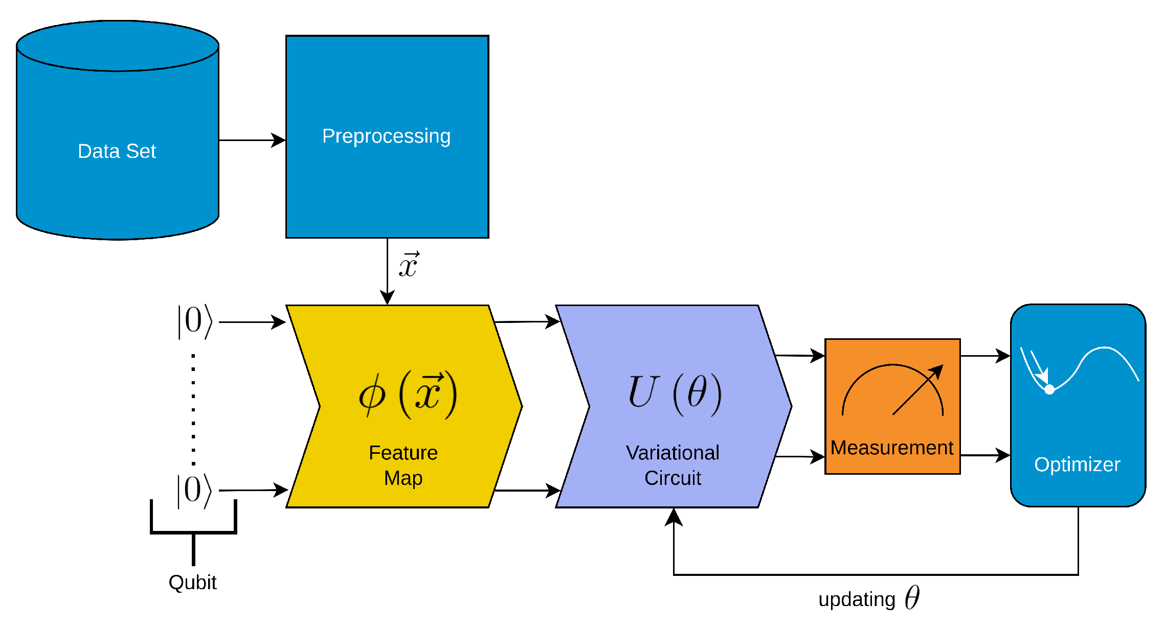
Figure 2.
Schematic depiction of the Quantum Kernel Estimator (QKE). The QKE consists of several steps. We colored the steps that are similar to classical support vector machines in light blue and the other steps in yellow and steel-blue. The employed QKE algorithm consists of a Support Vector Machine (SVM) algorithm with precomputed kernel, i.e. a classical machine learning method that leverages the power of quantum computing to efficiently compute the kernel matrix.
Figure 2.
Schematic depiction of the Quantum Kernel Estimator (QKE). The QKE consists of several steps. We colored the steps that are similar to classical support vector machines in light blue and the other steps in yellow and steel-blue. The employed QKE algorithm consists of a Support Vector Machine (SVM) algorithm with precomputed kernel, i.e. a classical machine learning method that leverages the power of quantum computing to efficiently compute the kernel matrix.
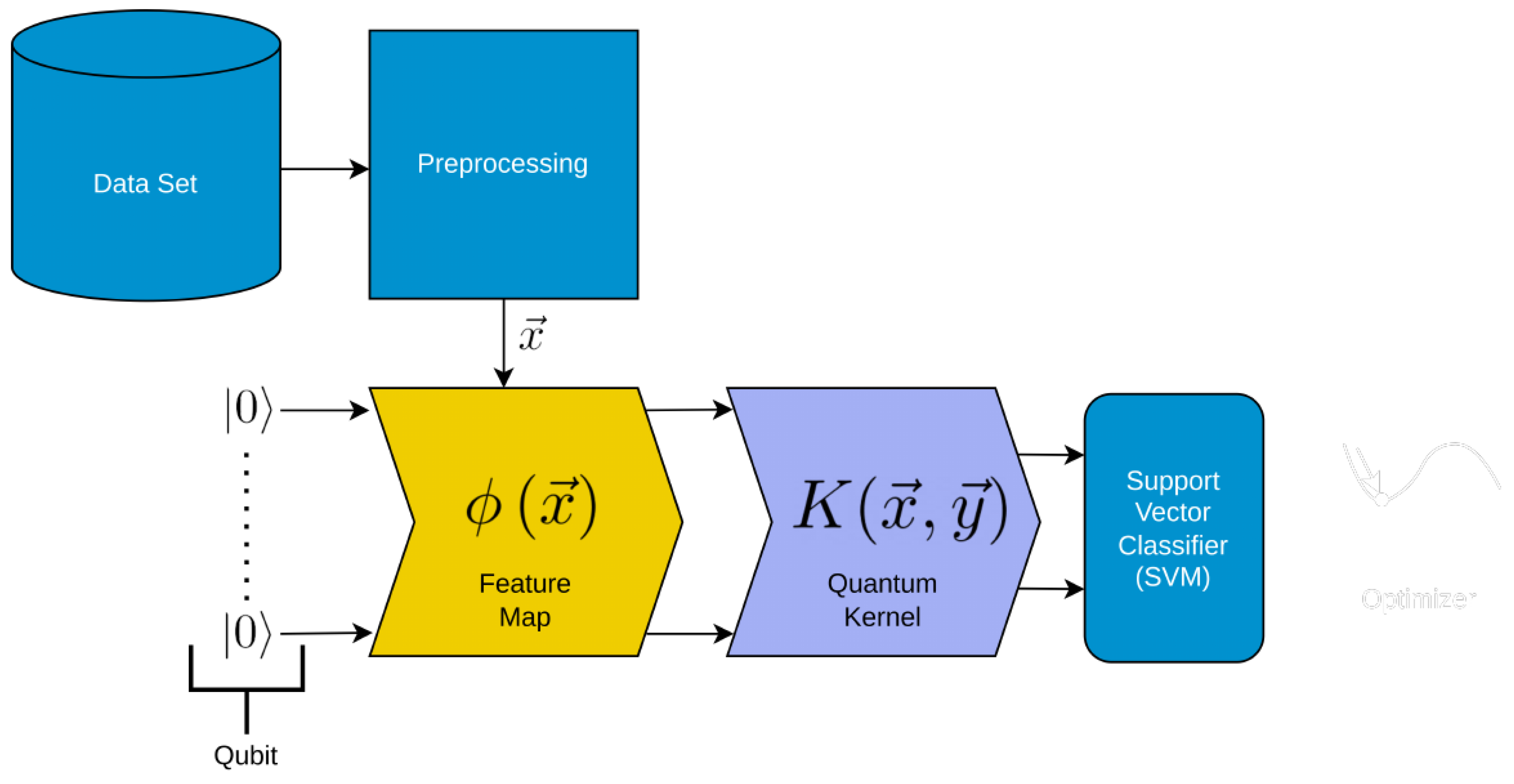
Figure 3.
These figures depict the results from our experiments, comparing the five best QML and classical ML algorithms on artificially generated datasets in terms of accuracy. The upper part illustrates the accuracy of the algorithms on different sample sizes, while the lower part demonstrates how the runtimes change with increasing size of the test dataset. The right part contains the legend, indicating which algorithms were used, and more specifically, the different parametrizations of the employed Quantum Machine Learning algorithms. Furthermore, the legend is sorted in decreasing order of the average accuracy of the employed algorithms. The parametrization for the QKE is as follows: QKE, Feature Map, Quantum Simulator, C-Value for the SVM-algorithm.
Figure 3.
These figures depict the results from our experiments, comparing the five best QML and classical ML algorithms on artificially generated datasets in terms of accuracy. The upper part illustrates the accuracy of the algorithms on different sample sizes, while the lower part demonstrates how the runtimes change with increasing size of the test dataset. The right part contains the legend, indicating which algorithms were used, and more specifically, the different parametrizations of the employed Quantum Machine Learning algorithms. Furthermore, the legend is sorted in decreasing order of the average accuracy of the employed algorithms. The parametrization for the QKE is as follows: QKE, Feature Map, Quantum Simulator, C-Value for the SVM-algorithm.
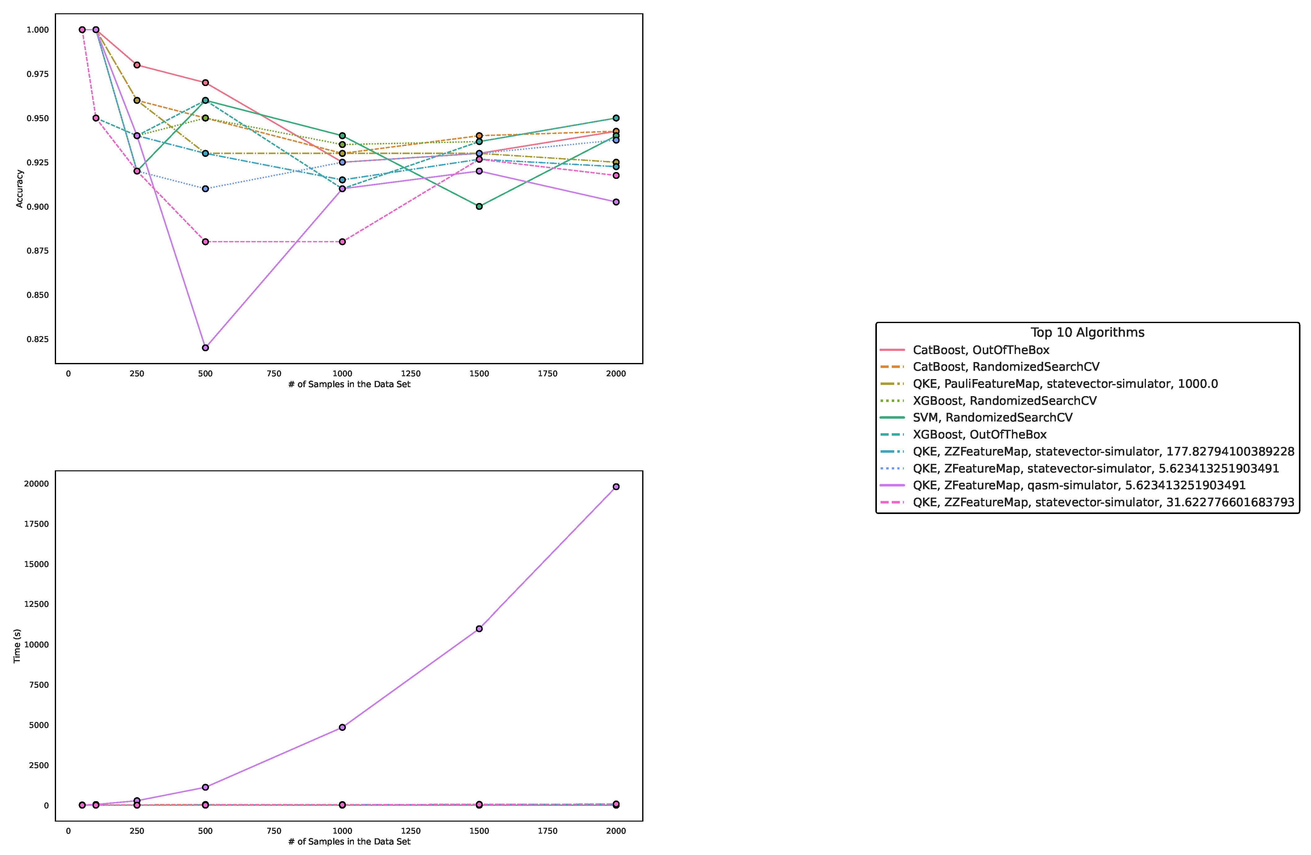
Figure 4.
These figures depict the results from our experiments, comparing differently parameterized classical machine learning algorithms on artificially generated datasets. The upper part illustrates the behavior of the accuracies, while the lower part demonstrates how the run times change with the increasing size of the test dataset. The right part contains the legend, indicating which algorithms were used, and more specifically, the different parametrizations of the employed Machine Learning algorithms. Furthermore, the legend is sorted in decreasing order of the average accuracy of the employed algorithms.
Figure 4.
These figures depict the results from our experiments, comparing differently parameterized classical machine learning algorithms on artificially generated datasets. The upper part illustrates the behavior of the accuracies, while the lower part demonstrates how the run times change with the increasing size of the test dataset. The right part contains the legend, indicating which algorithms were used, and more specifically, the different parametrizations of the employed Machine Learning algorithms. Furthermore, the legend is sorted in decreasing order of the average accuracy of the employed algorithms.
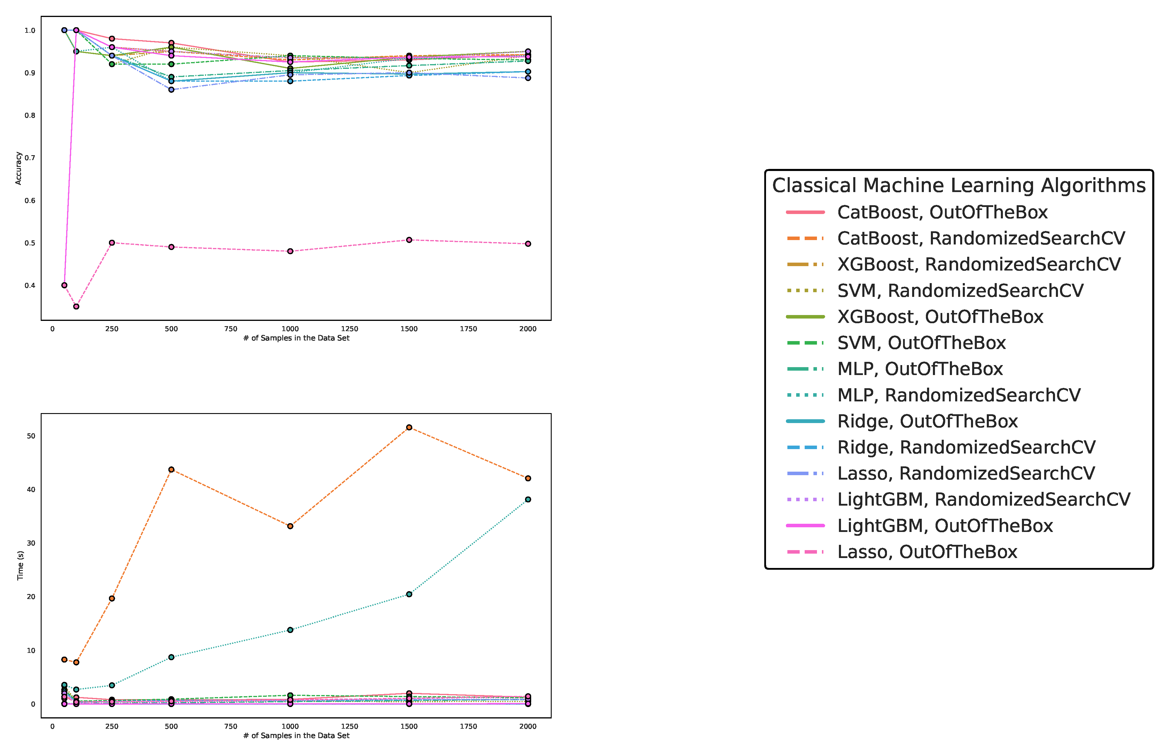
Figure 5.
These figures depict the results from our experiments for the artificially generated data sets, comparing differently parameterized QML algorithms on artificially generated datasets. The upper part illustrates the behavior of the accuracies, while the lower part demonstrates how the runtimes change with the increasing size of the test datasets. The right part contains the legend, indicating which algorithms were used, and more specifically, the different parametrizations of the employed Quantum Machine Learning algorithms. Furthermore, the legend is sorted in decreasing order of the average accuracy of the employed algorithms. The parametrization for the QKE is as follows: QKE, Feature Map, Quantum Simulator, C-Value for the SVM-Algorithm. The parametrization for the VQC is as follows: VQC, Feature Map, Ansatz, Optimizer, Quantum Simulator
Figure 5.
These figures depict the results from our experiments for the artificially generated data sets, comparing differently parameterized QML algorithms on artificially generated datasets. The upper part illustrates the behavior of the accuracies, while the lower part demonstrates how the runtimes change with the increasing size of the test datasets. The right part contains the legend, indicating which algorithms were used, and more specifically, the different parametrizations of the employed Quantum Machine Learning algorithms. Furthermore, the legend is sorted in decreasing order of the average accuracy of the employed algorithms. The parametrization for the QKE is as follows: QKE, Feature Map, Quantum Simulator, C-Value for the SVM-Algorithm. The parametrization for the VQC is as follows: VQC, Feature Map, Ansatz, Optimizer, Quantum Simulator
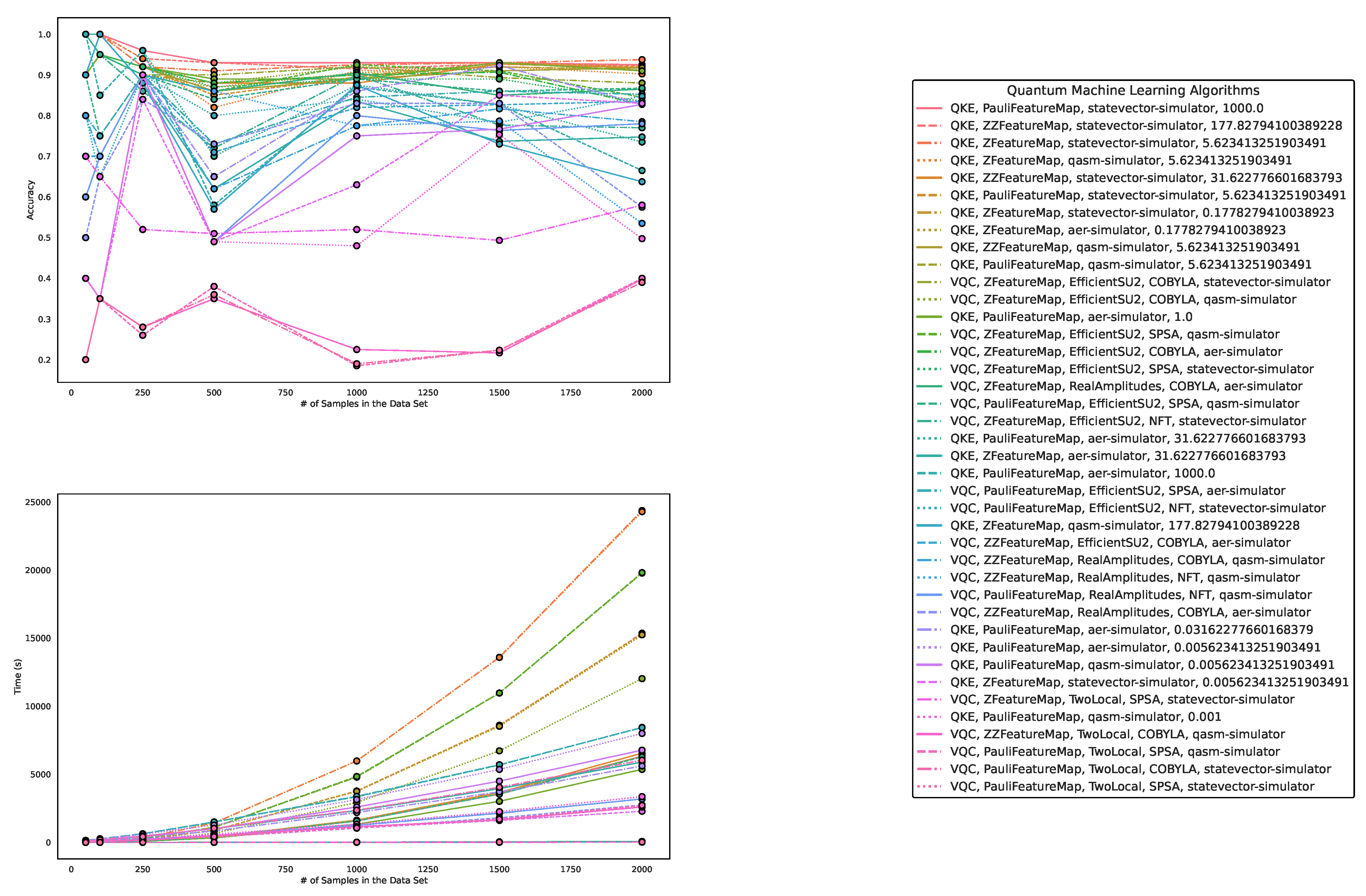
Figure 6.
These figures depict the results from our experiments, comparing the five best QML and classical ML algorithms in terms of accuracy on datasets using the exponential map to create -transformations on complex vectors. The upper part illustrates the accuracy of the algorithms on different sample sizes, while the lower part demonstrates how the runtimes change with the increasing size of the test dataset. The right part contains the legend, indicating which algorithms were used, and, more specifically, the different parametrizations of the employed Quantum Machine Learning algorithms. Furthermore, the legend is sorted in decreasing order of the average accuracy of the employed algorithms. The parametrization for the QKE is as follows: QKE, Feature Map, Quantum Simulator, C-Value for the SVM-algorithm.
Figure 6.
These figures depict the results from our experiments, comparing the five best QML and classical ML algorithms in terms of accuracy on datasets using the exponential map to create -transformations on complex vectors. The upper part illustrates the accuracy of the algorithms on different sample sizes, while the lower part demonstrates how the runtimes change with the increasing size of the test dataset. The right part contains the legend, indicating which algorithms were used, and, more specifically, the different parametrizations of the employed Quantum Machine Learning algorithms. Furthermore, the legend is sorted in decreasing order of the average accuracy of the employed algorithms. The parametrization for the QKE is as follows: QKE, Feature Map, Quantum Simulator, C-Value for the SVM-algorithm.
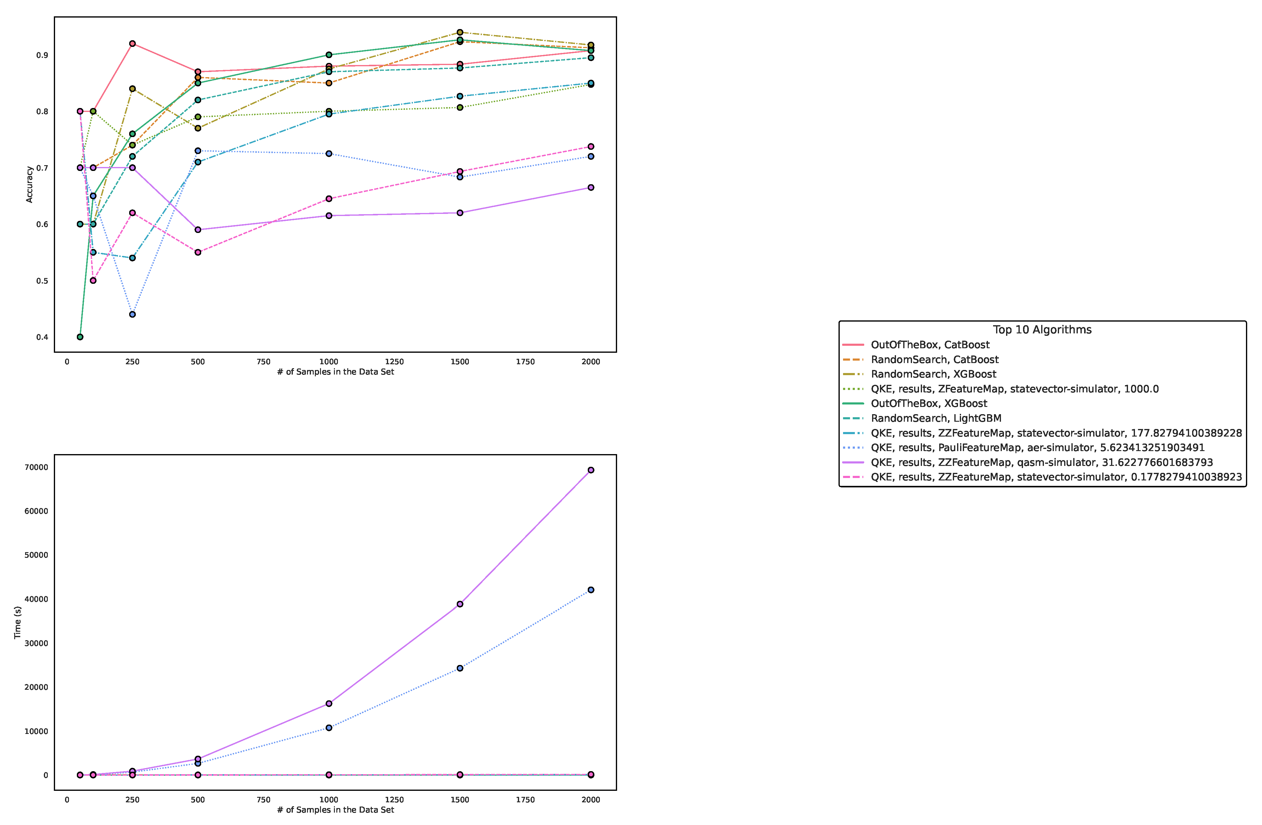
Figure 7.
These figures depict the results from our experiments, comparing differently parameterized classical machine learning algorithms on the -generated datasets. The upper part illustrates the behavior of the accuracies, while the lower part demonstrates how the run times change with the increasing size of the test dataset. The right part contains the legend, indicating which algorithms were used, and more specifically, the different parametrizations of the employed Machine Learning algorithms. Furthermore, the legend is sorted in decreasing order of the average accuracy of the employed algorithms.
Figure 7.
These figures depict the results from our experiments, comparing differently parameterized classical machine learning algorithms on the -generated datasets. The upper part illustrates the behavior of the accuracies, while the lower part demonstrates how the run times change with the increasing size of the test dataset. The right part contains the legend, indicating which algorithms were used, and more specifically, the different parametrizations of the employed Machine Learning algorithms. Furthermore, the legend is sorted in decreasing order of the average accuracy of the employed algorithms.
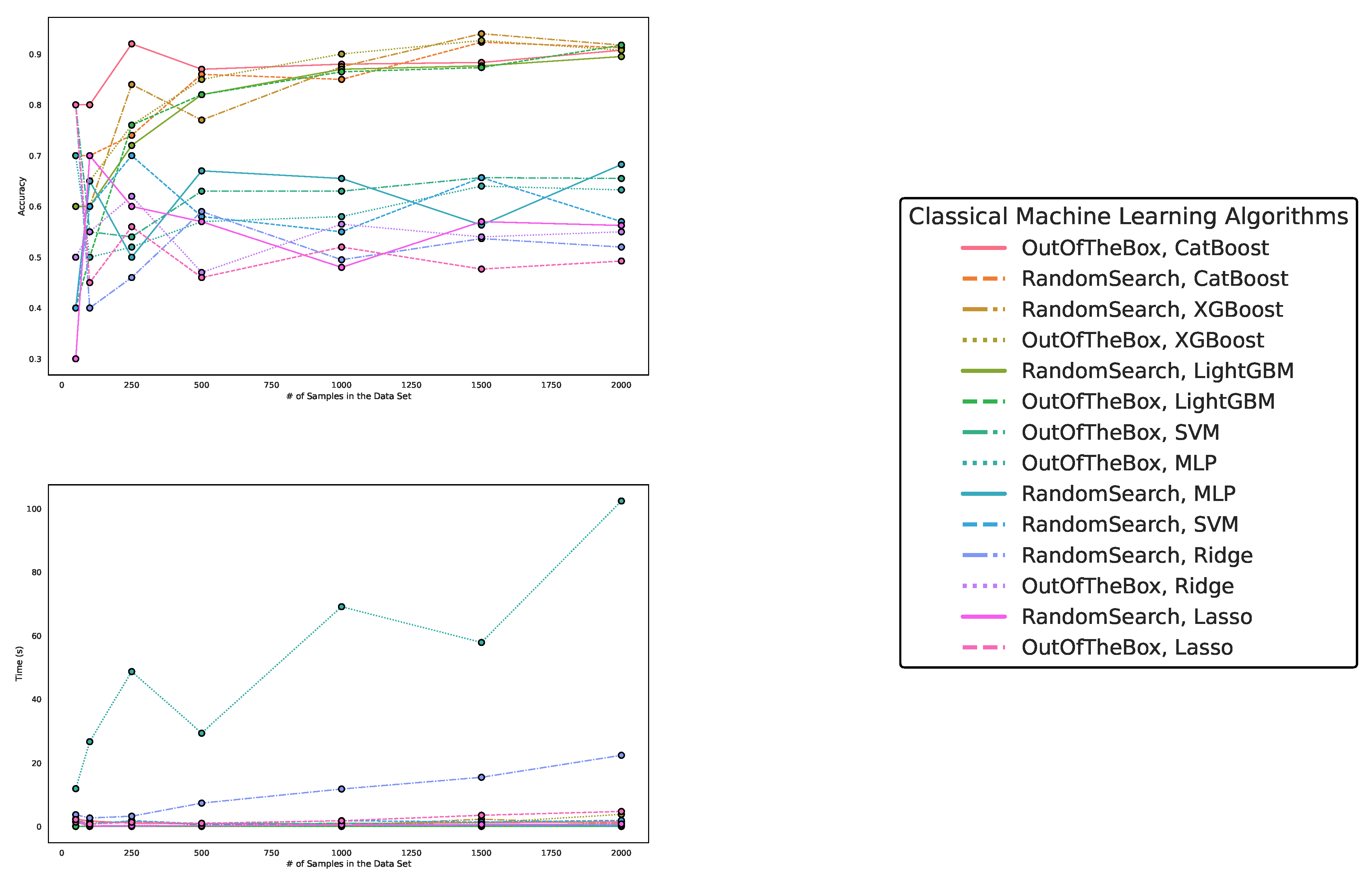
Figure 8.
These figures depict the results from our experiments for the artificially generated data sets, comparing differently parameterized QML algorithms on the -generated datasets. The upper part illustrates the behavior of the accuracies, while the lower part demonstrates how the runtimes change with the increasing size of the test datasets. The right part contains the legend, indicating which algorithms were used and, more specifically, the different parametrizations of the employed Quantum Machine Learning algorithms. Furthermore, the legend is sorted in decreasing order of the average accuracy of the employed algorithms. The parametrization for the QKE is as follows: QKE, Feature Map, Quantum Simulator, C-Value for the SVM-Algorithm. The parametrization for the VQC is as follows: VQC, Feature Map, Ansatz, Optimizer, Quantum Simulator.
Figure 8.
These figures depict the results from our experiments for the artificially generated data sets, comparing differently parameterized QML algorithms on the -generated datasets. The upper part illustrates the behavior of the accuracies, while the lower part demonstrates how the runtimes change with the increasing size of the test datasets. The right part contains the legend, indicating which algorithms were used and, more specifically, the different parametrizations of the employed Quantum Machine Learning algorithms. Furthermore, the legend is sorted in decreasing order of the average accuracy of the employed algorithms. The parametrization for the QKE is as follows: QKE, Feature Map, Quantum Simulator, C-Value for the SVM-Algorithm. The parametrization for the VQC is as follows: VQC, Feature Map, Ansatz, Optimizer, Quantum Simulator.
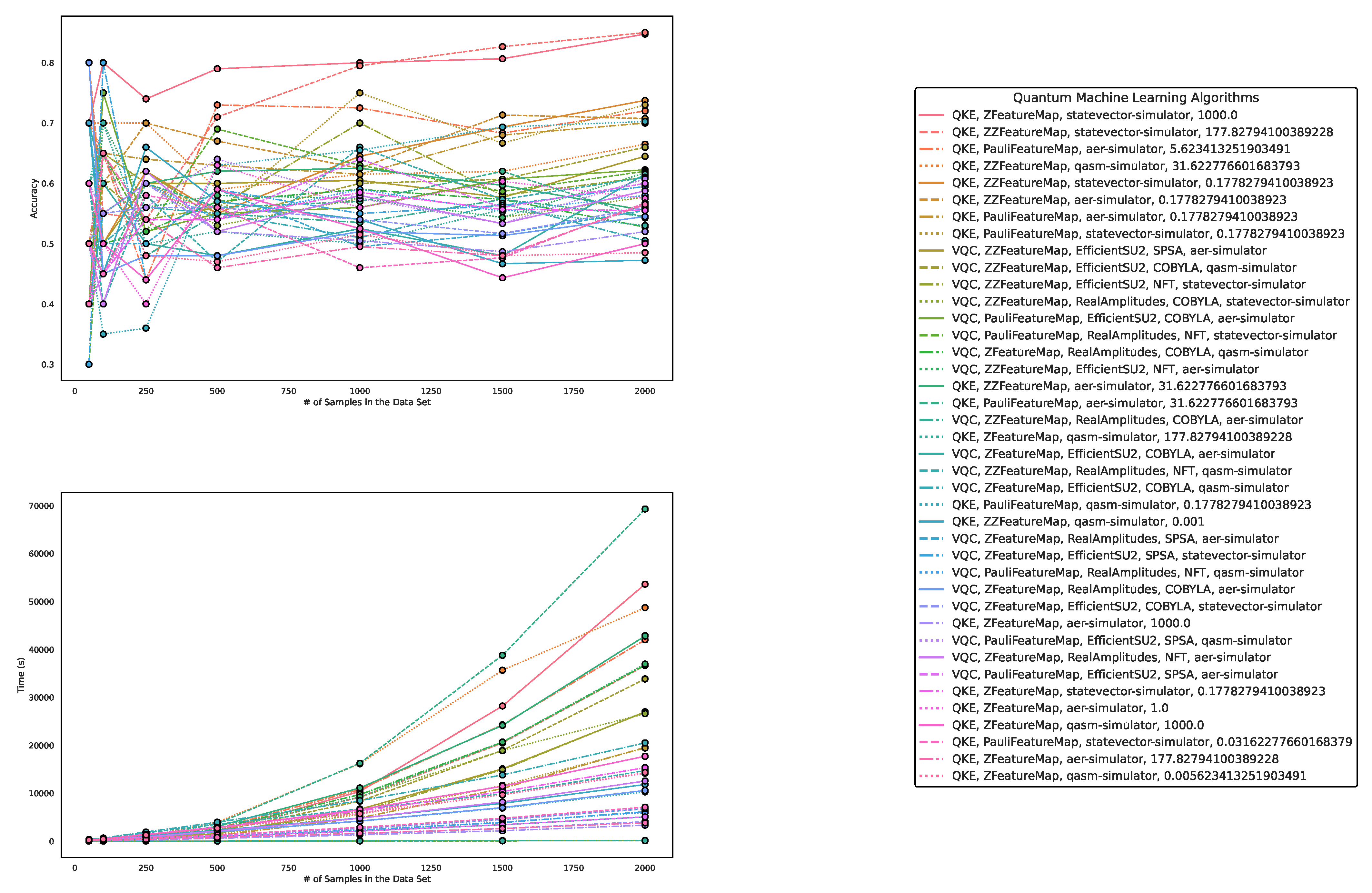

Table 1.
This table presents the scores/accuracies of our experiments conducted on artificially generated classification data sets. This table is sorted in decreasing order of the average accuracy over all sample sizes of each algorithm. The parametrization for the QKE is as follows: QKE, Feature Map, Quantum Simulator, C-Value for the SVM-Algorithm The parametrization for the VQC is as follows: VQC, Feature Map, Ansatz, Optimizer, Quantum Simulator
Table 1.
This table presents the scores/accuracies of our experiments conducted on artificially generated classification data sets. This table is sorted in decreasing order of the average accuracy over all sample sizes of each algorithm. The parametrization for the QKE is as follows: QKE, Feature Map, Quantum Simulator, C-Value for the SVM-Algorithm The parametrization for the VQC is as follows: VQC, Feature Map, Ansatz, Optimizer, Quantum Simulator
| Algorithm/Parametrization | Size 50 | Size 100 | Size 250 | Size 500 | Size 1000 | Size 1500 | Size 2000 | Average |
|---|---|---|---|---|---|---|---|---|
| CatBoost, OutOfTheBox | 1.0 | 1.0 | 0.98 | 0.97 | 0.925 | 0.93 | 0.9425 | 0.963929 |
| CatBoost, RandomizedSearchCV | 1.0 | 1.0 | 0.96 | 0.95 | 0.93 | 0.94 | 0.9425 | 0.960357 |
| QKE, PauliFeatureMap, statevector-simulator, 1000.0 | 1.0 | 1.0 | 0.96 | 0.93 | 0.93 | 0.93 | 0.925 | 0.953571 |
| XGBoost, RandomizedSearchCV | 1.0 | 0.95 | 0.94 | 0.95 | 0.935 | 0.936667 | 0.95 | 0.951667 |
| SVM, RandomizedSearchCV | 1.0 | 1.0 | 0.92 | 0.96 | 0.94 | 0.9 | 0.94 | 0.951429 |
| XGBoost, OutOfTheBox | 1.0 | 0.95 | 0.94 | 0.96 | 0.91 | 0.936667 | 0.95 | 0.949524 |
| SVM, OutOfTheBox | 1.0 | 1.0 | 0.92 | 0.92 | 0.94 | 0.933333 | 0.93 | 0.949048 |
| QKE, ZZFeatureMap, statevector-simulator, 177.82794100389228 | 1.0 | 1.0 | 0.94 | 0.93 | 0.915 | 0.926667 | 0.9225 | 0.947738 |
| QKE, ZFeatureMap, statevector-simulator, 5.623413251903491 | 1.0 | 1.0 | 0.92 | 0.91 | 0.925 | 0.93 | 0.9375 | 0.946071 |
| MLP, OutOfTheBox | 1.0 | 1.0 | 0.94 | 0.89 | 0.905 | 0.916667 | 0.9275 | 0.939881 |
| MLP, RandomizedSearchCV | 1.0 | 0.95 | 0.96 | 0.88 | 0.9 | 0.933333 | 0.94 | 0.937619 |
| Ridge, OutOfTheBox | 1.0 | 1.0 | 0.94 | 0.88 | 0.9 | 0.896667 | 0.9025 | 0.93131 |
| Ridge, RandomizedSearchCV | 1.0 | 1.0 | 0.94 | 0.88 | 0.88 | 0.893333 | 0.9025 | 0.927976 |
| QKE, ZFeatureMap, qasm-simulator, 5.623413251903491 | 1.0 | 1.0 | 0.94 | 0.82 | 0.91 | 0.92 | 0.9025 | 0.9275 |
| Lasso, RandomizedSearchCV | 1.0 | 1.0 | 0.94 | 0.86 | 0.895 | 0.9 | 0.8875 | 0.926071 |
| QKE, ZZFeatureMap, statevector-simulator, 31.622776601683793 | 1.0 | 0.95 | 0.92 | 0.88 | 0.88 | 0.926667 | 0.9175 | 0.924881 |
| QKE, PauliFeatureMap, statevector-simulator, 5.623413251903491 | 1.0 | 0.95 | 0.92 | 0.85 | 0.895 | 0.93 | 0.92 | 0.923571 |
| QKE, ZFeatureMap, statevector-simulator, 0.1778279410038923 | 1.0 | 0.95 | 0.9 | 0.88 | 0.9 | 0.92 | 0.9125 | 0.923214 |
| QKE, ZFeatureMap, aer-simulator, 0.1778279410038923 | 1.0 | 0.95 | 0.9 | 0.87 | 0.905 | 0.92 | 0.9125 | 0.9225 |
| QKE, ZZFeatureMap, qasm-simulator, 5.623413251903491 | 1.0 | 0.95 | 0.92 | 0.86 | 0.89 | 0.91 | 0.9175 | 0.921071 |
| QKE, PauliFeatureMap, qasm-simulator, 5.623413251903491 | 1.0 | 0.95 | 0.92 | 0.86 | 0.89 | 0.91 | 0.9175 | 0.921071 |
| VQC, ZFeatureMap, EfficientSU2, COBYLA, statevector-simulator | 1.0 | 0.95 | 0.9 | 0.9 | 0.92 | 0.893333 | 0.88 | 0.920476 |
| VQC, ZFeatureMap, EfficientSU2, COBYLA, qasm-simulator | 1.0 | 0.95 | 0.9 | 0.88 | 0.92 | 0.91 | 0.845 | 0.915 |
| QKE, PauliFeatureMap, aer-simulator, 1.0 | 0.9 | 0.95 | 0.92 | 0.89 | 0.89 | 0.93 | 0.91 | 0.912857 |
| VQC, ZFeatureMap, EfficientSU2, SPSA, qasm-simulator | 1.0 | 0.95 | 0.9 | 0.86 | 0.925 | 0.91 | 0.845 | 0.912857 |
| VQC, ZFeatureMap, EfficientSU2, COBYLA, aer-simulator | 1.0 | 0.95 | 0.92 | 0.88 | 0.9 | 0.906667 | 0.8275 | 0.912024 |
| VQC, ZFeatureMap, EfficientSU2, SPSA, statevector-simulator | 1.0 | 0.95 | 0.92 | 0.87 | 0.89 | 0.89 | 0.835 | 0.907857 |
| VQC, ZFeatureMap, RealAmplitudes, COBYLA, aer-simulator | 1.0 | 0.95 | 0.9 | 0.86 | 0.905 | 0.85 | 0.865 | 0.904286 |
| LightGBM, RandomizedSearchCV | 0.4 | 1.0 | 0.96 | 0.95 | 0.935 | 0.933333 | 0.95 | 0.875476 |
| LightGBM, OutOfTheBox | 0.4 | 1.0 | 0.96 | 0.94 | 0.925 | 0.936667 | 0.9375 | 0.87131 |
| VQC, PauliFeatureMap, EfficientSU2, SPSA, qasm-simulator | 0.9 | 0.75 | 0.9 | 0.84 | 0.89 | 0.86 | 0.8675 | 0.858214 |
| VQC, ZFeatureMap, EfficientSU2, NFT, statevector-simulator | 1.0 | 0.95 | 0.86 | 0.72 | 0.9 | 0.776667 | 0.77 | 0.85381 |
| QKE, PauliFeatureMap, aer-simulator, 31.622776601683793 | 1.0 | 0.85 | 0.96 | 0.7 | 0.875 | 0.826667 | 0.735 | 0.849524 |
| QKE, ZFeatureMap, aer-simulator, 31.622776601683793 | 1.0 | 1.0 | 0.88 | 0.62 | 0.835 | 0.736667 | 0.7475 | 0.83131 |
| QKE, PauliFeatureMap, aer-simulator, 1000.0 | 1.0 | 0.85 | 0.96 | 0.58 | 0.87 | 0.826667 | 0.665 | 0.821667 |
| VQC, PauliFeatureMap, EfficientSU2, SPSA, aer-simulator | 0.8 | 0.75 | 0.9 | 0.73 | 0.845 | 0.86 | 0.8525 | 0.819643 |
| VQC, PauliFeatureMap, EfficientSU2, NFT, statevector-simulator | 0.8 | 0.65 | 0.9 | 0.8 | 0.84 | 0.783333 | 0.8475 | 0.802976 |
| QKE, ZFeatureMap, qasm-simulator, 177.82794100389228 | 0.9 | 1.0 | 0.88 | 0.57 | 0.875 | 0.73 | 0.6375 | 0.798929 |
| VQC, ZZFeatureMap, EfficientSU2, COBYLA, aer-simulator | 0.7 | 0.7 | 0.9 | 0.71 | 0.82 | 0.826667 | 0.835 | 0.784524 |
| VQC, ZZFeatureMap, RealAmplitudes, COBYLA, qasm-simulator | 0.8 | 0.7 | 0.9 | 0.62 | 0.775 | 0.816667 | 0.785 | 0.770952 |
| VQC, ZZFeatureMap, RealAmplitudes, NFT, qasm-simulator | 0.7 | 0.7 | 0.9 | 0.86 | 0.775 | 0.786667 | 0.535 | 0.750952 |
| VQC, PauliFeatureMap, RealAmplitudes, NFT, qasm-simulator | 0.6 | 0.7 | 0.9 | 0.49 | 0.8 | 0.763333 | 0.78 | 0.719048 |
| VQC, ZZFeatureMap, RealAmplitudes, COBYLA, aer-simulator | 0.5 | 0.65 | 0.84 | 0.73 | 0.83 | 0.83 | 0.575 | 0.707857 |
| QKE, PauliFeatureMap, aer-simulator, 0.03162277660168379 | 0.4 | 0.35 | 0.9 | 0.65 | 0.86 | 0.923333 | 0.8275 | 0.701548 |
| QKE, PauliFeatureMap, aer-simulator, 0.005623413251903491 | 0.4 | 0.35 | 0.9 | 0.49 | 0.75 | 0.766667 | 0.8275 | 0.640595 |
| QKE, PauliFeatureMap, qasm-simulator, 0.005623413251903491 | 0.4 | 0.35 | 0.9 | 0.49 | 0.75 | 0.766667 | 0.8275 | 0.640595 |
| QKE, ZFeatureMap, statevector-simulator, 0.005623413251903491 | 0.4 | 0.35 | 0.84 | 0.49 | 0.63 | 0.85 | 0.83 | 0.627143 |
| VQC, ZFeatureMap, TwoLocal, SPSA, statevector-simulator | 0.7 | 0.65 | 0.52 | 0.51 | 0.52 | 0.493333 | 0.58 | 0.567619 |
| QKE, results, ZFeatureMap, qasm-simulator, 0.001 | 0.4 | 0.35 | 0.84 | 0.49 | 0.48 | 0.853333 | 0.4975 | 0.55869 |
| QKE, PauliFeatureMap, qasm-simulator, 0.001 | 0.4 | 0.35 | 0.9 | 0.49 | 0.48 | 0.753333 | 0.4975 | 0.552976 |
| Lasso, OutOfTheBox | 0.4 | 0.35 | 0.5 | 0.49 | 0.48 | 0.506667 | 0.4975 | 0.460595 |
| VQC, ZZFeatureMap, TwoLocal, COBYLA, qasm-simulator | 0.2 | 0.35 | 0.28 | 0.35 | 0.225 | 0.216667 | 0.3975 | 0.288452 |
| VQC, PauliFeatureMap, TwoLocal, SPSA, qasm-simulator | 0.2 | 0.35 | 0.26 | 0.38 | 0.185 | 0.223333 | 0.4 | 0.285476 |
| VQC, PauliFeatureMap, TwoLocal, COBYLA, statevector-simulator | 0.2 | 0.35 | 0.28 | 0.36 | 0.19 | 0.223333 | 0.39 | 0.284762 |
| VQC, PauliFeatureMap, TwoLocal, SPSA, statevector-simulator | 0.2 | 0.35 | 0.28 | 0.36 | 0.19 | 0.223333 | 0.39 | 0.284762 |
Table 2.
This table presents the run times in seconds of our experiments conducted on artificially generated classification data sets. This table is sorted in increasing order of the average runtimes over all sample sizes of each algorithm. The parametrization for the QKE is as follows: QKE, Feature Map, Quantum Simulator, C-Value for the SVM-Algorithm The parametrization for the VQC is as follows: VQC, Feature Map, Ansatz, Optimizer, Quantum Simulator
Table 2.
This table presents the run times in seconds of our experiments conducted on artificially generated classification data sets. This table is sorted in increasing order of the average runtimes over all sample sizes of each algorithm. The parametrization for the QKE is as follows: QKE, Feature Map, Quantum Simulator, C-Value for the SVM-Algorithm The parametrization for the VQC is as follows: VQC, Feature Map, Ansatz, Optimizer, Quantum Simulator
| Algorithm/Parametrization | Size 50 | Size 100 | Size 250 | Size 500 | Size 1000 | Size 1500 | Size 2000 | Average |
|---|---|---|---|---|---|---|---|---|
| Lasso, OutOfTheBox | 0.002163 | 0.000836 | 0.000638 | 0.000596 | 0.000571 | 0.000552 | 0.000575 | 0.000847 |
| Ridge, OutOfTheBox | 0.007653 | 0.001171 | 0.00121 | 0.001453 | 0.001333 | 0.00142 | 0.001452 | 0.002242 |
| SVM, OutOfTheBox | 0.001014 | 0.000671 | 0.001049 | 0.002419 | 0.003195 | 0.005537 | 0.012677 | 0.003795 |
| XGBoost, OutOfTheBox | 0.018497 | 0.008215 | 0.009782 | 0.021166 | 0.029465 | 0.032339 | 0.07877 | 0.028319 |
| LightGBM, OutOfTheBox | 0.013812 | 0.012791 | 0.01488 | 0.027696 | 0.054648 | 0.04419 | 0.054521 | 0.031791 |
| MLP, OutOfTheBox | 0.086815 | 0.090133 | 0.150594 | 0.231203 | 0.437073 | 0.647381 | 0.853657 | 0.356694 |
| SVM, RandomizedSearchCV | 1.993112 | 0.410673 | 0.468471 | 0.4341 | 0.658507 | 0.945457 | 0.896971 | 0.829613 |
| XGBoost, RandomizedSearchCV | 1.34873 | 0.358433 | 0.426441 | 0.519127 | 0.790996 | 1.049813 | 1.439898 | 0.847634 |
| Ridge, RandomizedSearchCV | 2.357919 | 0.298155 | 0.469647 | 0.706193 | 0.662371 | 0.774265 | 0.835577 | 0.872018 |
| Lasso, RandomizedSearchCV | 3.401839 | 0.482512 | 0.422395 | 0.473103 | 0.486651 | 0.438773 | 0.480838 | 0.88373 |
| CatBoost, OutOfTheBox | 1.045732 | 1.243495 | 0.812176 | 0.762516 | 0.865055 | 1.9962 | 1.268149 | 1.141903 |
| LightGBM, RandomizedSearchCV | 2.67037 | 0.536059 | 0.668838 | 0.900941 | 1.628797 | 1.389068 | 1.168039 | 1.280302 |
| VQC, ZFeatureMap, TwoLocal, SPSA, statevector-simulator | 0.502447 | 0.82391 | 1.319602 | 2.9078 | 6.75953 | 11.81601 | 18.064725 | 6.027718 |
| VQC, PauliFeatureMap, TwoLocal, COBYLA, statevector-simulator | 0.536454 | 0.886945 | 1.757877 | 3.486975 | 8.137821 | 14.688881 | 22.79476 | 7.469959 |
| VQC, PauliFeatureMap, TwoLocal, SPSA, statevector-simulator | 1.981785 | 0.715829 | 1.621059 | 3.488372 | 8.517624 | 15.170185 | 22.300972 | 7.685118 |
| VQC, PauliFeatureMap, TwoLocal, SPSA, qasm-simulator | 0.750719 | 1.154406 | 2.53449 | 5.000262 | 11.265137 | 19.493945 | 29.031463 | 9.89006 |
| VQC, ZZFeatureMap, TwoLocal, COBYLA, qasm-simulator | 0.734865 | 1.097202 | 2.514703 | 4.990832 | 11.895971 | 19.283406 | 29.318269 | 9.976464 |
| MLP, RandomizedSearchCV | 3.568304 | 2.701256 | 3.490188 | 8.736222 | 13.817605 | 20.424873 | 38.117078 | 12.979361 |
| QKE, ZFeatureMap, statevector-simulator, 0.1778279410038923 | 1.343983 | 0.802286 | 2.170829 | 5.965899 | 18.504546 | 36.659922 | 59.889941 | 17.905344 |
| QKE, ZFeatureMap, statevector-simulator, 0.005623413251903491 | 0.411296 | 0.697461 | 2.154164 | 6.122564 | 19.670819 | 37.297334 | 62.1901 | 18.363391 |
| QKE, PauliFeatureMap, statevector-simulator, 1000.0 | 0.470933 | 0.956269 | 2.721257 | 7.2817 | 21.356298 | 40.130716 | 67.422908 | 20.048583 |
| QKE, PauliFeatureMap, statevector-simulator, 5.623413251903491 | 0.501446 | 0.922237 | 2.775664 | 7.454642 | 21.780637 | 40.426036 | 66.758927 | 20.088513 |
| QKE, ZFeatureMap, statevector-simulator, 5.623413251903491 | 0.378018 | 0.757363 | 2.141677 | 4.962464 | 19.901565 | 41.913003 | 71.453831 | 20.215417 |
| QKE, ZZFeatureMap, statevector-simulator, 31.622776601683793 | 0.214386 | 0.567282 | 1.650304 | 5.302437 | 20.77629 | 42.614517 | 72.871078 | 20.570899 |
| QKE, ZZFeatureMap, statevector-simulator, 177.82794100389228 | 0.461093 | 0.943574 | 2.780804 | 7.580857 | 22.906811 | 41.955521 | 68.045553 | 20.667745 |
| CatBoost, RandomizedSearchCV | 8.292872 | 7.778893 | 19.636858 | 43.697806 | 33.126305 | 51.559816 | 42.05208 | 29.449233 |
| VQC, ZFeatureMap, RealAmplitudes, COBYLA, aer-simulator | 47.438183 | 63.446748 | 192.148143 | 404.233954 | 1060.291657 | 1619.397205 | 2290.222381 | 811.025467 |
| VQC, ZZFeatureMap, RealAmplitudes, COBYLA, qasm-simulator | 43.113636 | 83.175558 | 166.040938 | 421.278374 | 1064.238564 | 1702.893006 | 2719.340939 | 885.725859 |
| VQC, ZZFeatureMap, RealAmplitudes, COBYLA, aer-simulator | 45.909504 | 83.201411 | 152.20265 | 509.1956 | 1158.902532 | 1654.065907 | 2603.942577 | 886.774312 |
| VQC, ZFeatureMap, EfficientSU2, COBYLA, statevector-simulator | 48.546243 | 81.030425 | 190.958188 | 402.121722 | 1044.855825 | 1807.676357 | 2751.241623 | 903.775769 |
| VQC, ZFeatureMap, EfficientSU2, COBYLA, aer-simulator | 57.728111 | 100.590997 | 240.174666 | 507.58709 | 1253.080578 | 2139.855218 | 3196.07247 | 1070.727019 |
| VQC, ZFeatureMap, EfficientSU2, COBYLA, qasm-simulator | 59.058898 | 100.862056 | 242.285405 | 507.171731 | 1262.650143 | 2151.503499 | 3191.745568 | 1073.611043 |
| VQC, ZZFeatureMap, EfficientSU2, COBYLA, aer-simulator | 59.651649 | 105.629842 | 254.918442 | 601.245125 | 1335.017904 | 2260.354294 | 3366.65501 | 1140.496038 |
| QKE, ZFeatureMap, qasm-simulator, 177.82794100389228 | 4.589478 | 13.184805 | 82.633779 | 332.71327 | 1337.102907 | 3020.689579 | 5368.201509 | 1451.30219 |
| QKE, ZZFeatureMap, qasm-simulator, 5.623413251903491 | 4.352785 | 15.921249 | 97.165028 | 390.472092 | 1573.103197 | 3549.629798 | 6282.670251 | 1701.902057 |
| QKE, PauliFeatureMap, aer-simulator, 0.03162277660168379 | 3.549125 | 15.094144 | 98.970568 | 393.496921 | 1581.662241 | 3554.962927 | 6317.355669 | 1709.298799 |
| QKE, PauliFeatureMap, aer-simulator, 0.005623413251903491 | 3.373257 | 15.311538 | 99.2351 | 390.52131 | 1574.108371 | 3555.3048 | 6339.026443 | 1710.982974 |
| QKE, PauliFeatureMap, qasm-simulator, 0.005623413251903491 | 3.812115 | 19.479307 | 101.289711 | 404.432384 | 1636.24686 | 3642.937393 | 6307.605039 | 1730.828973 |
| QKE, PauliFeatureMap, aer-simulator, 31.622776601683793 | 3.848578 | 17.062982 | 101.387533 | 408.69903 | 1635.863136 | 3674.976257 | 6555.811507 | 1771.092718 |
| VQC, ZFeatureMap, EfficientSU2, NFT, statevector-simulator | 98.831974 | 167.48274 | 394.378037 | 836.913451 | 2197.652135 | 3719.047116 | 5621.134708 | 1862.205737 |
| VQC, PauliFeatureMap, EfficientSU2, NFT, statevector-simulator | 103.914165 | 177.047181 | 423.423603 | 1014.963511 | 2338.078356 | 3953.861723 | 5905.433094 | 1988.10309 |
| VQC, ZZFeatureMap, RealAmplitudes, NFT, qasm-simulator | 105.987181 | 183.918751 | 427.016702 | 1036.605473 | 2366.463152 | 4052.521035 | 6042.538015 | 2030.721473 |
| VQC, PauliFeatureMap, RealAmplitudes, NFT, qasm-simulator | 103.625823 | 180.306618 | 425.488049 | 1041.160999 | 2371.366715 | 4044.856475 | 6048.573929 | 2030.768373 |
| VQC, ZFeatureMap, EfficientSU2, SPSA, statevector-simulator | 119.513477 | 200.101417 | 474.113288 | 1008.932874 | 2601.731917 | 4505.306268 | 6781.089745 | 2241.541284 |
| VQC, ZFeatureMap, EfficientSU2, SPSA, qasm-simulator | 145.295744 | 256.711762 | 609.791229 | 1272.675059 | 3150.527537 | 5366.116602 | 8009.649075 | 2687.25243 |
| VQC, PauliFeatureMap, EfficientSU2, SPSA, aer-simulator | 144.280811 | 259.102175 | 625.193096 | 1502.476923 | 3356.340799 | 5689.827615 | 8454.144295 | 2861.623673 |
| VQC, PauliFeatureMap, EfficientSU2, SPSA, qasm-simulator | 152.666649 | 269.680847 | 642.400747 | 1505.762521 | 3388.662998 | 5709.505826 | 8438.957709 | 2872.519614 |
| QKE, ZFeatureMap, aer-simulator, 31.622776601683793 | 5.993241 | 25.852654 | 166.703792 | 669.201309 | 2934.169598 | 6729.31411 | 12037.430687 | 3224.095056 |
| QKE, results, ZFeatureMap, qasm-simulator, 0.001 | 6.277584 | 25.986847 | 166.57816 | 669.951543 | 2961.024113 | 6778.469155 | 11992.12485 | 3228.630322 |
| QKE, PauliFeatureMap, qasm-simulator, 5.623413251903491 | 8.384715 | 32.795287 | 206.595473 | 890.414904 | 3753.488868 | 8537.768589 | 15232.745542 | 4094.599054 |
| QKE, PauliFeatureMap, qasm-simulator, 0.001 | 7.792093 | 32.566225 | 207.832614 | 896.042249 | 3778.324351 | 8610.335147 | 15348.810142 | 4125.957546 |
| QKE, ZFeatureMap, aer-simulator, 0.1778279410038923 | 10.511296 | 43.335078 | 276.810734 | 1111.545614 | 4799.032996 | 10979.135601 | 19768.073574 | 5284.063556 |
| QKE, ZFeatureMap, qasm-simulator, 5.623413251903491 | 11.573929 | 43.186982 | 277.291314 | 1113.664313 | 4842.587094 | 10978.908476 | 19798.821156 | 5295.147609 |
| QKE, PauliFeatureMap, aer-simulator, 1000.0 | 12.596938 | 51.788837 | 332.281104 | 1434.208601 | 5986.631006 | 13592.866065 | 24280.544075 | 6527.273804 |
| QKE, PauliFeatureMap, aer-simulator, 1.0 | 12.261604 | 51.508959 | 332.561822 | 1423.111135 | 5984.902587 | 13603.956887 | 24362.83202 | 6538.733573 |
Table 3.
This table presents the scores/accuracies of our experiments conducted on artificially generated classification data sets. This table is sorted in decreasing order of the average accuracy over all sample sizes of each algorithm. The parametrization for the QKE is as follows: QKE, Feature Map, Quantum Simulator, C-Value for the SVM-Algorithm The parametrization for the VQC is as follows: VQC, Feature Map, Ansatz, Optimizer, Quantum Simulator
Table 3.
This table presents the scores/accuracies of our experiments conducted on artificially generated classification data sets. This table is sorted in decreasing order of the average accuracy over all sample sizes of each algorithm. The parametrization for the QKE is as follows: QKE, Feature Map, Quantum Simulator, C-Value for the SVM-Algorithm The parametrization for the VQC is as follows: VQC, Feature Map, Ansatz, Optimizer, Quantum Simulator
| Algorithm/Parametrization | Size 50 | Size 100 | Size 250 | Size 500 | Size 1000 | Size 1500 | Size 2000 | Average |
|---|---|---|---|---|---|---|---|---|
| OutOfTheBox, CatBoost | 0.8 | 0.8 | 0.92 | 0.87 | 0.88 | 0.883333 | 0.9075 | 0.865833 |
| RandomSearch, CatBoost | 0.7 | 0.7 | 0.74 | 0.86 | 0.85 | 0.923333 | 0.9125 | 0.812262 |
| RandomSearch, XGBoost | 0.6 | 0.6 | 0.84 | 0.77 | 0.875 | 0.94 | 0.9175 | 0.791786 |
| QKE, ZFeatureMap, statevector-simulator, 1000.0 | 0.7 | 0.8 | 0.74 | 0.79 | 0.8 | 0.806667 | 0.8475 | 0.783452 |
| OutOfTheBox, XGBoost | 0.4 | 0.65 | 0.76 | 0.85 | 0.9 | 0.926667 | 0.9075 | 0.770595 |
| RandomSearch, LightGBM | 0.6 | 0.6 | 0.72 | 0.82 | 0.87 | 0.876667 | 0.895 | 0.76881 |
| OutOfTheBox, LightGBM | 0.4 | 0.5 | 0.76 | 0.82 | 0.865 | 0.873333 | 0.9175 | 0.73369 |
| QKE, ZZFeatureMap, statevector-simulator, 177.82794100389228 | 0.8 | 0.55 | 0.54 | 0.71 | 0.795 | 0.826667 | 0.85 | 0.724524 |
| QKE, PauliFeatureMap, aer-simulator, 5.623413251903491 | 0.7 | 0.65 | 0.44 | 0.73 | 0.725 | 0.683333 | 0.72 | 0.664048 |
| QKE, ZZFeatureMap, qasm-simulator, 31.622776601683793 | 0.7 | 0.7 | 0.7 | 0.59 | 0.615 | 0.62 | 0.665 | 0.655714 |
| QKE, ZZFeatureMap, statevector-simulator, 0.1778279410038923 | 0.8 | 0.5 | 0.62 | 0.55 | 0.645 | 0.693333 | 0.7375 | 0.649405 |
| OutOfTheBox, SVM | 0.8 | 0.55 | 0.54 | 0.63 | 0.63 | 0.656667 | 0.655 | 0.637381 |
| QKE, ZZFeatureMap, aer-simulator, 0.1778279410038923 | 0.4 | 0.6 | 0.7 | 0.67 | 0.625 | 0.713333 | 0.7075 | 0.630833 |
| QKE, PauliFeatureMap, aer-simulator, 0.1778279410038923 | 0.5 | 0.65 | 0.64 | 0.63 | 0.615 | 0.68 | 0.7 | 0.630714 |
| QKE, PauliFeatureMap, statevector-simulator, 0.1778279410038923 | 0.4 | 0.65 | 0.6 | 0.55 | 0.75 | 0.666667 | 0.73 | 0.620952 |
| VQC, ZZFeatureMap, EfficientSU2, SPSA, aer-simulator | 0.7 | 0.5 | 0.6 | 0.6 | 0.605 | 0.576667 | 0.645 | 0.60381 |
| VQC, ZZFeatureMap, EfficientSU2, COBYLA, qasm-simulator | 0.6 | 0.6 | 0.62 | 0.54 | 0.6 | 0.606667 | 0.66 | 0.60381 |
| OutOfTheBox, MLP | 0.7 | 0.5 | 0.52 | 0.57 | 0.58 | 0.64 | 0.6325 | 0.591786 |
| RandomSearch, MLP | 0.4 | 0.65 | 0.5 | 0.67 | 0.655 | 0.563333 | 0.6825 | 0.58869 |
| VQC, ZZFeatureMap, EfficientSU2, NFT, statevector-simulator | 0.5 | 0.6 | 0.54 | 0.56 | 0.7 | 0.58 | 0.61 | 0.584286 |
| VQC, ZZFeatureMap, RealAmplitudes, COBYLA, statevector-simulator | 0.6 | 0.65 | 0.6 | 0.53 | 0.575 | 0.543333 | 0.5775 | 0.582262 |
| RandomSearch, SVM | 0.4 | 0.6 | 0.7 | 0.58 | 0.55 | 0.656667 | 0.57 | 0.579524 |
| VQC, PauliFeatureMap, EfficientSU2, COBYLA, aer-simulator | 0.4 | 0.75 | 0.52 | 0.55 | 0.56 | 0.606667 | 0.6225 | 0.572738 |
| VQC, PauliFeatureMap, RealAmplitudes, NFT, statevector-simulator | 0.3 | 0.65 | 0.52 | 0.69 | 0.63 | 0.586667 | 0.62 | 0.570952 |
| VQC, ZFeatureMap, RealAmplitudes, COBYLA, qasm-simulator | 0.7 | 0.5 | 0.52 | 0.57 | 0.59 | 0.573333 | 0.5275 | 0.56869 |
| VQC, ZZFeatureMap, EfficientSU2, NFT, aer-simulator | 0.4 | 0.7 | 0.56 | 0.58 | 0.575 | 0.543333 | 0.6175 | 0.567976 |
| QKE, ZZFeatureMap, aer-simulator, 31.622776601683793 | 0.4 | 0.55 | 0.6 | 0.62 | 0.625 | 0.596667 | 0.555 | 0.56381 |
| QKE, PauliFeatureMap, aer-simulator, 31.622776601683793 | 0.6 | 0.45 | 0.6 | 0.56 | 0.57 | 0.62 | 0.5425 | 0.563214 |
| VQC, ZZFeatureMap, RealAmplitudes, COBYLA, aer-simulator | 0.6 | 0.65 | 0.48 | 0.55 | 0.535 | 0.573333 | 0.545 | 0.561905 |
| QKE, ZFeatureMap, qasm-simulator, 177.82794100389228 | 0.6 | 0.7 | 0.5 | 0.52 | 0.5 | 0.556667 | 0.53 | 0.558095 |
| VQC, ZFeatureMap, EfficientSU2, COBYLA, aer-simulator | 0.7 | 0.6 | 0.5 | 0.48 | 0.525 | 0.48 | 0.615 | 0.557143 |
| VQC, ZZFeatureMap, RealAmplitudes, NFT, qasm-simulator | 0.6 | 0.4 | 0.58 | 0.47 | 0.66 | 0.573333 | 0.61 | 0.55619 |
| VQC, ZFeatureMap, EfficientSU2, COBYLA, qasm-simulator | 0.7 | 0.5 | 0.56 | 0.55 | 0.51 | 0.566667 | 0.505 | 0.555952 |
| QKE, PauliFeatureMap, qasm-simulator, 0.1778279410038923 | 0.5 | 0.35 | 0.36 | 0.63 | 0.655 | 0.693333 | 0.7025 | 0.555833 |
| QKE, ZZFeatureMap, qasm-simulator, 0.001 | 0.7 | 0.45 | 0.66 | 0.57 | 0.54 | 0.466667 | 0.4725 | 0.55131 |
| VQC, ZFeatureMap, RealAmplitudes, SPSA, aer-simulator | 0.7 | 0.5 | 0.5 | 0.59 | 0.495 | 0.516667 | 0.555 | 0.550952 |
| VQC, ZFeatureMap, EfficientSU2, SPSA, statevector-simulator | 0.3 | 0.8 | 0.44 | 0.59 | 0.55 | 0.563333 | 0.595 | 0.548333 |
| VQC, PauliFeatureMap, RealAmplitudes, NFT, qasm-simulator | 0.4 | 0.55 | 0.6 | 0.54 | 0.59 | 0.553333 | 0.58 | 0.544762 |
| RandomSearch, Ridge | 0.8 | 0.4 | 0.46 | 0.59 | 0.495 | 0.536667 | 0.52 | 0.543095 |
| OutOfTheBox, Ridge | 0.5 | 0.55 | 0.62 | 0.47 | 0.565 | 0.54 | 0.55 | 0.542143 |
| VQC, ZFeatureMap, RealAmplitudes, COBYLA, aer-simulator | 0.8 | 0.45 | 0.48 | 0.48 | 0.52 | 0.513333 | 0.545 | 0.54119 |
| VQC, ZFeatureMap, EfficientSU2, COBYLA, statevector-simulator | 0.5 | 0.55 | 0.56 | 0.56 | 0.54 | 0.516667 | 0.56 | 0.540952 |
| RandomSearch, Lasso | 0.3 | 0.7 | 0.6 | 0.57 | 0.48 | 0.57 | 0.5625 | 0.540357 |
| QKE, ZFeatureMap, aer-simulator, 1000.0 | 0.6 | 0.55 | 0.6 | 0.52 | 0.505 | 0.486667 | 0.52 | 0.540238 |
| VQC, PauliFeatureMap, EfficientSU2, SPSA, qasm-simulator | 0.4 | 0.45 | 0.56 | 0.64 | 0.575 | 0.533333 | 0.6075 | 0.537976 |
| OutOfTheBox, Lasso | 0.8 | 0.45 | 0.56 | 0.46 | 0.52 | 0.476667 | 0.4925 | 0.537024 |
| VQC, ZFeatureMap, RealAmplitudes, NFT, aer-simulator | 0.5 | 0.4 | 0.62 | 0.52 | 0.58 | 0.533333 | 0.5875 | 0.534405 |
| VQC, PauliFeatureMap, EfficientSU2, SPSA, aer-simulator | 0.4 | 0.45 | 0.54 | 0.54 | 0.64 | 0.56 | 0.6 | 0.532857 |
| QKE, ZFeatureMap, statevector-simulator, 0.1778279410038923 | 0.5 | 0.45 | 0.54 | 0.54 | 0.585 | 0.556667 | 0.555 | 0.532381 |
| QKE, ZFeatureMap, aer-simulator, 1.0 | 0.4 | 0.5 | 0.4 | 0.63 | 0.56 | 0.603333 | 0.575 | 0.524048 |
| QKE, ZFeatureMap, qasm-simulator, 1000.0 | 0.6 | 0.5 | 0.44 | 0.59 | 0.525 | 0.443333 | 0.5 | 0.514048 |
| QKE, PauliFeatureMap, statevector-simulator, 0.03162277660168379 | 0.5 | 0.45 | 0.58 | 0.56 | 0.46 | 0.476667 | 0.5675 | 0.513452 |
| QKE, ZFeatureMap, aer-simulator, 177.82794100389228 | 0.4 | 0.65 | 0.54 | 0.46 | 0.495 | 0.48 | 0.565 | 0.512857 |
| QKE, ZFeatureMap, qasm-simulator, 0.005623413251903491 | 0.5 | 0.65 | 0.48 | 0.47 | 0.515 | 0.48 | 0.485 | 0.511429 |
Table 4.
This table presents the run times in seconds of our experiments conducted on artificially generated classification data sets. This table is sorted in increasing order of the average runtimes over all sample sizes of each algorithm. The parametrization for the QKE is as follows: QKE, Feature Map, Quantum Simulator, C-Value for the SVM-Algorithm The parametrization for the VQC is as follows: VQC, Feature Map, Ansatz, Optimizer, Quantum Simulator
Table 4.
This table presents the run times in seconds of our experiments conducted on artificially generated classification data sets. This table is sorted in increasing order of the average runtimes over all sample sizes of each algorithm. The parametrization for the QKE is as follows: QKE, Feature Map, Quantum Simulator, C-Value for the SVM-Algorithm The parametrization for the VQC is as follows: VQC, Feature Map, Ansatz, Optimizer, Quantum Simulator
| Algorithm/Parametrization | Size 50 | Size 100 | Size 250 | Size 500 | Size 1000 | Size 1500 | Size 2000 | Average |
|---|---|---|---|---|---|---|---|---|
| OutOfTheBox, Lasso | 0.000775 | 0.000667 | 0.000917 | 0.000745 | 0.000764 | 0.001107 | 0.000657 | 0.000805 |
| OutOfTheBox, Ridge | 0.003182 | 0.002283 | 0.001883 | 0.001916 | 0.002109 | 0.001808 | 0.002117 | 0.002185 |
| OutOfTheBox, SVM | 0.001026 | 0.000899 | 0.002106 | 0.00511 | 0.01778 | 0.034653 | 0.062489 | 0.017723 |
| RandomSearch, Lasso | 2.182304 | 0.182914 | 0.176461 | 0.244406 | 0.441368 | 0.344652 | 0.169867 | 0.534567 |
| RandomSearch, SVM | 1.388398 | 0.164014 | 0.227862 | 0.224122 | 0.497012 | 0.616385 | 0.791133 | 0.558418 |
| RandomSearch, Ridge | 1.592006 | 0.205837 | 0.172721 | 0.237846 | 0.502149 | 0.525089 | 0.724933 | 0.565797 |
| OutOfTheBox, LightGBM | 0.034643 | 0.045887 | 0.144432 | 0.329458 | 0.362766 | 2.262915 | 0.904509 | 0.583516 |
| OutOfTheBox, XGBoost | 1.564661 | 1.002106 | 1.577685 | 0.592689 | 1.008408 | 0.408685 | 0.302948 | 0.922455 |
| OutOfTheBox, MLP | 0.112287 | 0.11116 | 0.333941 | 0.222378 | 0.969315 | 1.129416 | 3.801408 | 0.954272 |
| OutOfTheBox, CatBoost | 2.362274 | 1.712796 | 1.057932 | 0.864497 | 0.948283 | 1.209606 | 1.46414 | 1.374218 |
| RandomSearch, LightGBM | 2.29224 | 0.691731 | 1.831599 | 0.835876 | 1.822398 | 1.40603 | 1.906817 | 1.540956 |
| RandomSearch, XGBoost | 2.173722 | 0.746218 | 1.348106 | 1.018472 | 1.797382 | 3.524122 | 4.735716 | 2.191963 |
| RandomSearch, MLP | 3.705261 | 2.66241 | 3.235272 | 7.354552 | 11.794682 | 15.48622 | 22.415577 | 9.521996 |
| QKE, ZFeatureMap, statevector-simulator, 1000.0 | 0.588803 | 1.105112 | 3.115228 | 9.692818 | 24.488245 | 46.863381 | 75.605305 | 23.065556 |
| QKE, ZZFeatureMap, statevector-simulator, 177.82794100389228 | 1.023377 | 2.014738 | 6.133744 | 14.08855 | 36.209869 | 63.510698 | 97.575217 | 31.508028 |
| QKE, PauliFeatureMap, statevector-simulator, 0.1778279410038923 | 1.110054 | 2.154783 | 6.591036 | 14.487802 | 36.089562 | 62.912848 | 97.64273 | 31.569831 |
| QKE, ZFeatureMap, statevector-simulator, 0.1778279410038923 | 1.235019 | 1.984607 | 5.547594 | 15.333808 | 41.977686 | 79.052726 | 127.710628 | 38.977438 |
| QKE, PauliFeatureMap, statevector-simulator, 0.03162277660168379 | 1.453579 | 2.804056 | 9.085313 | 19.440721 | 47.633347 | 81.740004 | 128.186636 | 41.477665 |
| QKE, ZZFeatureMap, statevector-simulator, 0.1778279410038923 | 2.194236 | 4.856549 | 10.043207 | 20.391739 | 57.658834 | 97.515617 | 151.070676 | 49.104408 |
| RandomSearch, CatBoost | 11.89935 | 26.694282 | 48.668876 | 29.36561 | 69.105261 | 57.845912 | 102.396539 | 49.425119 |
| VQC, ZFeatureMap, RealAmplitudes, COBYLA, qasm-simulator |
55.500573 | 100.423827 | 241.59017 | 577.400258 | 1286.962867 | 2164.282246 | 3315.185871 | 1105.906545 |
| VQC, ZFeatureMap, RealAmplitudes, COBYLA, aer-simulatorr |
61.174412 | 116.296597 | 274.944359 | 672.215972 | 1509.987298 | 2624.710516 | 4058.819283 | 1331.164062 |
| VQC, ZZFeatureMap, RealAmplitudes, COBYLA, statevector-simulator |
68.600875 | 123.207802 | 380.446356 | 770.716185 | 1635.89919 | 2621.242822 | 3805.021206 | 1343.590634 |
| VQC, PauliFeatureMap, EfficientSU2, COBYLA, aer-simulator |
89.832315 | 163.70887 | 480.279572 | 975.291255 | 2084.174564 | 3407.844934 | 5050.433405 | 1750.223559 |
| VQC, ZZFeatureMap, EfficientSU2, COBYLA, qasm-simulator |
88.21128 | 163.988243 | 480.35886 | 973.614566 | 2068.950356 | 3425.564759 | 5057.849761 | 1751.219689 |
| VQC, ZFeatureMap, EfficientSU2, COBYLA, qasm-simulator |
85.847133 | 156.496491 | 381.392026 | 888.461174 | 2300.527629 | 3878.06995 | 6136.175247 | 1975.281379 |
| VQC, ZFeatureMap, EfficientSU2, COBYLA, statevector-simulator |
103.51928 | 191.066923 | 456.017277 | 1079.39181 | 2305.444005 | 3940.212229 | 5958.277453 | 2004.846997 |
| VQC, ZFeatureMap, RealAmplitudes, NFT, aer-simulator |
111.03018 | 203.235006 | 491.978903 | 1181.668828 | 2620.544781 | 4428.84701 | 6770.538213 | 2258.263274 |
| VQC, ZFeatureMap, EfficientSU2, COBYLA, aer-simulator |
113.765615 | 205.589837 | 516.289881 | 1202.288662 | 2663.121947 | 4533.378097 | 6730.84663 | 2280.754381 |
| VQC, ZZFeatureMap, RealAmplitudes, COBYLA, aer-simulator |
111.686165 | 209.034186 | 638.294179 | 1296.48554 | 2869.708946 | 4781.981067 | 7074.925479 | 2426.016509 |
| VQC, PauliFeatureMap, RealAmplitudes, NFT, qasm-simulator |
163.24924 | 303.991817 | 936.898012 | 1915.698994 | 4145.466983 | 6900.43208 | 10273.374065 | 3519.873027 |
| VQC, ZFeatureMap, EfficientSU2, SPSA, statevector-simulator |
190.048137 | 341.454534 | 823.875859 | 1930.637818 | 4188.237967 | 6999.258807 | 10586.6448 | 3580.02256 |
| VQC, PauliFeatureMap, RealAmplitudes, NFT, statevector-simulator |
190.485358 | 349.906865 | 1108.180672 | 2248.345232 | 4814.143806 | 7883.610885 | 11821.059517 | 4059.390334 |
| VQC, ZFeatureMap, RealAmplitudes, SPSA, aer-simulator |
195.45132 | 357.101921 | 856.679886 | 2110.857992 | 4766.449826 | 8178.593323 | 12549.799371 | 4144.99052 |
| VQC, ZZFeatureMap, RealAmplitudes, NFT, qasm-simulator |
224.602174 | 405.497928 | 1270.741552 | 2674.141109 | 5725.217252 | 9676.191547 | 14306.04881 | 4897.491482 |
| VQC, ZZFeatureMap, EfficientSU2, NFT, statevector-simulator |
243.54281 | 457.172266 | 1372.528644 | 2784.422174 | 5896.297166 | 9666.126191 | 14179.331314 | 4942.774366 |
| QKE, ZFeatureMap, aer-simulator, 1.0 |
9.847104 | 40.399745 | 258.379268 | 1171.612393 | 4847.638381 | 10994.736629 | 19569.132042 | 5270.249366 |
| VQC, ZZFeatureMap, EfficientSU2, NFT, aer-simulator |
259.240503 | 473.126474 | 1408.601057 | 2903.563737 | 6301.786963 | 10332.959201 | 15345.314436 | 5289.227482 |
| VQC, PauliFeatureMap, EfficientSU2, SPSA, aer-simulator |
316.140029 | 574.301472 | 1727.700192 | 3530.722918 | 6706.076042 | 9861.491595 | 14726.388476 | 5348.974389 |
| QKE, ZFeatureMap, aer-simulator, 1000.0 |
10.898171 | 46.773357 | 297.390107 | 1339.784466 | 5587.107904 | 11607.623344 | 19440.97092 | 5475.79261 |
| VQC, ZZFeatureMap, EfficientSU2, SPSA, aer-simulator |
243.897139 | 463.586231 | 1368.88324 | 2789.133991 | 6570.676821 | 11456.705765 | 17726.796588 | 5802.811396 |
| VQC, PauliFeatureMap, EfficientSU2, SPSA, qasm-simulator |
348.216144 | 639.131772 | 1898.469802 | 3945.807249 | 8437.848893 | 13815.446673 | 20511.034176 | 7085.136387 |
| QKE, ZFeatureMap, qasm-simulator, 1000.0 |
11.579451 | 47.675482 | 344.543775 | 1568.903939 | 6191.830912 | 14908.467701 | 27002.766078 | 7153.681048 |
| QKE, ZFeatureMap, aer-simulator, 177.82794100389228 |
14.163619 | 56.856619 | 359.793343 | 1620.482626 | 6647.990849 | 15084.137764 | 26961.326713 | 7249.250219 |
| QKE, ZFeatureMap, qasm-simulator, 177.82794100389228 | 16.35717 | 77.129608 | 482.478877 | 2237.68152 | 9219.954344 | 18899.046552 | 26623.312487 | 8222.28008 |
| QKE, ZFeatureMap, qasm-simulator, 0.005623413251903491 | 16.184459 | 68.030962 | 439.889123 | 2003.14586 | 8339.157072 | 18939.866418 | 33875.189822 | 9097.351959 |
| QKE, PauliFeatureMap, aer-simulator, 31.622776601683793 | 16.822446 | 70.391611 | 549.285996 | 2267.794391 | 9148.306499 | 20490.131389 | 36687.638808 | 9890.05302 |
| QKE, ZZFeatureMap, aer-simulator, 31.622776601683793 | 17.382234 | 70.921393 | 552.720236 | 2290.305118 | 9223.01824 | 20681.450668 | 36991.554065 | 9975.335993 |
| QKE, ZZFeatureMap, aer-simulator, 0.1778279410038923 | 19.618006 | 80.653612 | 632.012298 | 2628.407038 | 9714.431489 | 20666.725844 | 36766.378776 | 10072.603866 |
| QKE, PauliFeatureMap, aer-simulator, 5.623413251903491 | 20.03461 | 81.805468 | 657.437384 | 2646.600018 | 10751.043722 | 24303.410594 | 42050.186601 | 11501.502628 |
| QKE, ZZFeatureMap, qasm-simulator, 0.001 | 22.474871 | 94.5939 | 748.53639 | 3061.492908 | 11095.037557 | 24179.108494 | 42833.544061 | 11719.255454 |
| QKE, PauliFeatureMap, aer-simulator, 0.1778279410038923 | 15.70449 | 64.293166 | 539.372432 | 2052.767245 | 10360.381735 | 28219.134103 | 53610.138579 | 13551.684536 |
| QKE, PauliFeatureMap, qasm-simulator, 0.1778279410038923 | 28.777769 | 121.675706 | 961.248534 | 3951.052992 | 16159.343561 | 35692.431334 | 48691.262451 | 15086.541764 |
| QKE, ZZFeatureMap, qasm-simulator, 31.622776601683793 | 28.201021 | 110.795119 | 877.141222 | 3647.413017 | 16257.207805 | 38819.796065 | 69300.661749 | 18434.459428 |
Table 5.
These tables present the scores/accuracies of our experiments conducted on publicly available classification datasets. The upper table displays the best 5-fold cross-validation scores, obtained using Randomized Search cross-validation from Scikit-learn, which were employed to identify the optimal model. The lower table shows the scores of the best model evaluated on an unseen test subset of the original data. We include results for the six datasets described in Section 2.5, the quantum classifiers detailed in Section 2.3, and the classical machine learning classifiers discussed in Section 2.2.
Table 5.
These tables present the scores/accuracies of our experiments conducted on publicly available classification datasets. The upper table displays the best 5-fold cross-validation scores, obtained using Randomized Search cross-validation from Scikit-learn, which were employed to identify the optimal model. The lower table shows the scores of the best model evaluated on an unseen test subset of the original data. We include results for the six datasets described in Section 2.5, the quantum classifiers detailed in Section 2.3, and the classical machine learning classifiers discussed in Section 2.2.
| Classifier\Dataset | Iris | Wine | ILPD | BC-Coimbra | TAE | Breast-Tissue |
|---|---|---|---|---|---|---|
| VQC | 0.817 | 0.817 | 0.706 | 0.599 | 0.417 | 0.339 |
| QKE | 0.908 | 0.853 | 0.706 | 0.620 | 0.483 | 0.382 |
| Ridge | 0.914 | 0.875 | 0.080 | 0.053 | 0.053 | <0.001 |
| Lasso | 0.914 | 0.870 | 0.085 | 0.004 | 0.004 | <0.001 |
| MLP | 0.975 | 0.937 | 0.712 | 0.687 | 0.425 | 0.406 |
| SVM | 0.958 | 0.759 | 0.706 | 0.630 | 0.450 | 0.382 |
| XGBoost | 0.958 | 0.986 | 0.695 | 0.656 | 0.533 | 0.441 |
| LightGBM | 0.967 | 0.986 | 0.699 | 0.666 | 0.475 | 0.393 |
| CatBoost | 0.950 | 0.979 | 0.702 | 0.688 | 0.525 | 0.440 |
| Classifier\Dataset | Iris | Wine | ILPD | BC-Coimbra | TAE | Breast-Tissue |
| VQC | 0.767 | 0.639 | 0.744 | 0.541 | 0.388 | 0.334 |
| QKE | 1.0 | 0.833 | 0.744 | 0.792 | 0.613 | 0.409 |
| Ridge | 0.947 | 0.878 | 0.115 | 0.234 | <0.001 | <0.001 |
| Lasso | 0.945 | 0.882 | 0.115 | 0.296 | <0.001 | <0.001 |
| MLP | 1.0 | 1.0 | 0.769 | 0.875 | 0.387 | 0.455 |
| SVM | 1.0 | 0.972 | 0.743 | 0.875 | 0.355 | 0.455 |
| XGBoost | 1.0 | 1.0 | 0.735 | 0.917 | 0.533 | 0.441 |
| LightGBM | 1.0 | 1.0 | 0.752 | 0.917 | 0.419 | 0.455 |
| CatBoost | 1.0 | 1.0 | 0.744 | 0.917 | 0.645 | 0.545 |
Table 6.
This table presents the combined runtimes of our experiments conducted on well-known and publicly available classification datasets. The runtimes include both the 5-fold Randomized Search cross-validation process from Scikit-learn, which was employed to identify the optimal model, and the evaluation of the best model on an unseen test subset of the original data. We include results for the six datasets described in Section 2.5, the quantum classifiers detailed in Section 2.3, and the classical machine learning classifiers discussed in Section 2.2.
Table 6.
This table presents the combined runtimes of our experiments conducted on well-known and publicly available classification datasets. The runtimes include both the 5-fold Randomized Search cross-validation process from Scikit-learn, which was employed to identify the optimal model, and the evaluation of the best model on an unseen test subset of the original data. We include results for the six datasets described in Section 2.5, the quantum classifiers detailed in Section 2.3, and the classical machine learning classifiers discussed in Section 2.2.
| Classifier\ Dataset |
Iris | Wine | ILPD | BC-Coimbra | TAE | Breast-Tissue |
|---|---|---|---|---|---|---|
| VQC | 3:32:16.547605 | 1 day, 13:56:59.455185 | 2 days, 23:03:26.398856 | 9:55:17.907443 | 2:46:25.921553 | 9:01:58.623806 |
| QKE | 2:03:57.921154 | 21:41:38.738255 | 7 days, 6:30:41.179676 | 5:02:26.430001 | 1:28:54.069725 | 3:37:05.655104 |
| Ridge | 0:00:00.175009 | 0:00:00.496771 | 0:00:00.399229 | 0:00:00.240857 | 0:00:00.209600 | 0:00:00.296966 |
| Lasso | 0:00:00.173051 | 0:00:00.181444 | 0:00:00.237455 | 0:00:00.192257 | 0:00:00.229508 | 0:00:00.225531 |
| MLP | 0:00:16.876288 | 0:00:10.477420 | 0:00:26.748907 | 0:00:10.951229 | 0:00:08.475263 | 0:00:13.729790 |
| SVM | 0:00:00.143353 | 0:00:00.165431 | 0:00:00.484485 | 0:00:00.180694 | 0:00:00.228508 | 0:00:00.226784 |
| XGBoost | 0:00:03.809085 | 0:00:04.030425 | 0:00:04.752627 | 0:00:02.744122 | 0:00:05.820371 | 0:00:06.864497 |
| LightGBM | 0:00:02.971164 | 0:00:03.180770 | 0:00:03.062553 | 0:00:01.462174 | 0:00:03.056615 | 0:00:04.540870 |
| CatBoost | 0:00:06.465975 | 0:00:18.511612 | 0:00:11.352944 | 0:00:07.460460 | 0:00:06.964821 | 0:00:26.639070 |
Disclaimer/Publisher’s Note: The statements, opinions and data contained in all publications are solely those of the individual author(s) and contributor(s) and not of MDPI and/or the editor(s). MDPI and/or the editor(s) disclaim responsibility for any injury to people or property resulting from any ideas, methods, instructions or products referred to in the content. |
© 2023 by the authors. Licensee MDPI, Basel, Switzerland. This article is an open access article distributed under the terms and conditions of the Creative Commons Attribution (CC BY) license (http://creativecommons.org/licenses/by/4.0/).
Copyright: This open access article is published under a Creative Commons CC BY 4.0 license, which permit the free download, distribution, and reuse, provided that the author and preprint are cited in any reuse.


