
Submitted:
10 May 2023
Posted:
11 May 2023
You are already at the latest version
Abstract
Since its original publication 1 in 1978, Lozi’s chaotic map has been thoroughly explored and continues to be. Hundreds of publications analyze its particular structure or apply its properties in many fields (electronic devices like memristor, A.I. with swarm intelligence, etc.). Several generalizations have been proposed, transforming the initial two-dimensional map into multidimensional one. However, they do not respect the original constraint that allows this map to be one of the few strictly hyperbolic: a constant Jacobian. In this paper we introduce a three-dimensional piece-wise linear extension respecting this constraint and we explore a special property never highlighted for chaotic mappings: the coexistence of thread-chaotic attractors (i.e., attractors which are formed by collection of lines) and sheet-chaotic attractors (i.e., attractors which are formed by collection of planes). This new 3-dimensional mapping can generate a large variety of chaotic and hyperchaotic attractors. We give five examples of such behavior in this article. In the first three examples, there is coexistence of thread and sheet-chaotic attractors. However, their shape are different and they are constituted by a different number of pieces. In the two last examples, the blow up of the attractors with respect to parameter a and b is highlighted.
Keywords:
chaotic attractor
; hyperchaotic attractor
; Lozi map
; sheet-attractor
; thread-attractor
1. Introduction
Since its original publication in 1978, Lozi’s chaotic map has been thoroughly explored and continues to be. Hundreds of publications analyze its particular structure or apply its properties in many fields (cryptography, optimization, secure communications, electronic devices like memristor, A.I. with swarm intelligence, etc.). Several kinds of generalization have been proposed, transforming the initial two-dimensional map into multidimensional. However, they do not respect the original constraint that allows this map to be one of the few strictly hyperbolic: a constant Jacobian. In this paper we introduce a three-dimensional piece-wise linear extension respecting this constraint and we explore a special property never highlighted for chaotic mappings: the coexistence of thread-chaotic attractors (i.e., attractors which are formed by collection of lines) and sheet-hyperchaotic attractors which are formed by collection of planes).
In Section 2, we recall the history and initial defin(i.e., attractorsition of the Lozi map, its chaotic properties in the dissipative case, the dynamics features (fixed points, invariant manifolds, basin of attraction, etc.). We describe also the chaotic properties in the conservative case. We do a rapid survey of the generalization of such map: topological generalizations (Lozi-like map), geometrical generalization (Lozi-type map), generalization of the formula in dimension 3 or more, fractal generalization, non-conventional generalization and networks of Lozi maps with chimera. In Section 3 we recall the definition of two Ros̎sler hyperchaotic attractors for comparison, and we introduce a new generalization fo the Lozi map in three dimensions. In Section 4 we give the basic properties of the thread and sheet-attractors (fixed point, period-two orbit). This new 3-dimensional mapping can generate a large variety of chaotic and hyperchaotic attractors. We give five examples of such behavior in this section. In the first three examples, there is coexistence of thread and sheet chaotic attractors. However, their shape are different and they are constituted by a different number of pieces. In the two last examples, the blow up of the attractors with respect to parameter a and b is highlighted. A brief conclusion is drawn in Section 5.
2. The Lozi map
2.1. History
The Lozi map was found by René Lozi exactly on 15 June 1977 around 11 am during the defense of the Ph. D. thesis of one of his colleague in the department of mathematics of the University of Nice (France) [1] (p. xxv).
As he explained in [2], the week before, he attended the International Conference on Mathematical Problems in Theoretical Physics in Roma. The opening talk was given by David Ruelle on 6 June, who conjectured in his presentation that, for the Hénon attractor, the theoretical entropy should be equal to the characteristic exponent [3]. This is how he discovered the first example of chaotic and strange attractors (See Figure 1).
Hénon who explored numerically the Lorenz map [4] using a IBM-7040 found it difficult to highlight its inner nature due to its very strong dissipativity. Its rate of volume contraction is given by the Lie derivative of the Lorenz equations which can be solved. For the parameters chosen by Lorenz, . Therefore, after one time unit, volumes are reduced by a factor . Inspired by his astronomer experience of Poincaré’s map for the motion of planets, Hénon built the metaphoric model [5]
also represented by the iterates of any initial point by the map
For this map the contracting properties are only determined by the parameter b. With , the contraction in one iteration is mild enough that the sheaves of the attractors are visible. Eventually he observed graphically the fractal structure of the attractor which astonished the research community.
2.1.1. Initial definition
At this time, Lozi was working in numerical analysis, in the domain of bifurcation which was not very developed in France. His main interest was focused on discretization problem and finite element method in which nonlinear functions are approximated by piecewise linear ones. During the Roma conference, he tried unsuccessfully to apply the spirit of the method of finite element to the Hénon attractor. Back to Nice after this conference, he eventually decided, using paper and pencil, to change the square function of the Hénon attractor, which is U shaped, into the absolute value function, which has a V shape, implying folding property (folding property is important for horseshoe a main ingredient of chaos, as highlighted by Stephen Smale [6]).
2.1.2. Chaotic properties of the dissipative map (|b|<1)
When the map is called "dissipative" that means that the image of any subset by f has a measure which is less than the measure of : .
Two years after the discovery of this new chaotic attractor and only one year after its publication [7], at the end of 1979, during the International Conference on Nonlinear Dynamics, patronized by the New-York Academy of Sciences on December 17-21, 1979, Michal Misiurewicz, presented a rigorous proof that for a set of parameters this map has a strange attractor, coining at this occasion the name `Lozi map’ [8]. This set in the plane of parameters is defined by (See Figure 3).
2.1.3. Fixed points, invariant manifolds and basin of attraction
Due to the piecewise linearity of absolute value in (3), one can compute explicitly the fixed points and the periodic orbit of any order of it.
When ( for both regions and are in the cone defined by theses inequalities), there exist two fixed points
which belongs to the quadrant , and
which belongs to the quadrant .
Furthermore, one can easily compute the local stability of these points by evaluating the corresponding eigenvalues of the Jacobian matrix of , and conclude that, in the domain of the parameter space where both and coexist, that is, for , they are saddle points.
Interestingly, the chaotic attractor of the Lozi map belongs to the unstable invariant manifold of . More exactly from [8] it is known that the chaotic (and strange) attractor can be constructed from the successive forward iterations of a trapping region F,
with F the triangle with vertices at the points I, , and , where I is the point given by the intersection of the unstable manifold of the fixed point with the horizontal axis,
Baptista et al. [11] have found that the basin of attractor is modeled by some parts of the stable manifold of the fixed point . They consider the point X intersection of this stable manifold with the vertical axis. A simple computation gives its expression as
and a certain point T belonging on the horizontal axis, first defined by Ishii [12] whose expression is
They show that the basin of attraction is bounded by a polygonal line entirely characterized by the points T, X and their successive preimages.
2.1.4. Other dynamical properties of the dissipative map (|b|<1)
Boroński, Kucharski and Ou [13] rigorously determined an open region in the parameter space for which Lozi map exhibits periodic points of least period n, for all .
and
where , , , ,
and .
Theorem 1
([13]). For all the Lozi map has a periodic point of least period n, for and all .
It is not in the scope of this article to provide a survey of all the papers describing the other dynamical or statistical properties of the Lozi map, because they are too numerous. One may refer to [1] for a compendium of results published between 1997 to 2013. Below, only some particular or more recent results are pointed out.
Many authors have published results on bifurcations of such map, like Botella-Soler et al. [14] showing that it presents what they call bisecting bifurcations: those which are mediated by an infinite set of neutrally stable periodic orbits.
Sushko et al. [15] investigate the bifurcation structure of the parameter plane in the vicinity of the curve related to a center bifurcation of the fixed point. A distinguishing property of the Lozi map is that it is conservative (see Section 2.1.5) at the parameter value corresponding to this bifurcation. As a result, the bifurcation structure close to the center bifurcation curve is quite complicated. In particular, an attracting fixed point (focus) can coexist with various attracting cycles, as well as with chaotic attractors, and the number of coexisting attractors increases as the parameter point approaches the center bifurcation curve. Their study contributes also to the border collision bifurcation theory since the Lozi map is a particular case of the 2D border collision normal form (2D-BCNF).
Glendinning and Simpson [16] use as canonical example the following 2D-BCNF which is the family of difference equations
and with
They restrict in their paper their attention to the parameter values , , , , , for which f is invertible and orientation-preserving.
The role of is to control the border-collision bifurcation. In view of a linear rescaling, it is only needed to consider it for the values (here it is 1). The condition is needed for the definition of the induced map. If and then the 2d BCNF reduces to the Lozi map.
In addition of bifurcation studies, Collet and Levy [17] consider ergodic properties of such mapping, that they consider as intermediate stage between the Axiom A dynamical systems and more complicated systems like the Hénon map. They construct its Bowen-Ruelle measure and also derive some of its properties which are similar to those of an axiom A system.
Rychlik [18] gives a proof of the existence of Sinai-Bowen-Ruelle measures (SBR measures) for this map. He also proves that the number of SBR measures is finite.
Cao and Liu [19] explore the geometric structure of its chaotic attractor and proof:
Proposition 1.
If the parameters satisfy Misiurewicz conditions (4), then the strange attractor possesses the following properties:
- -
- The union of the transversal homoclinic points and weak transversal homoclinic points are dense in .
- -
- All periodic points are hyperbolic.
- -
- The set of periodic points forms a dense set in .
- -
- Any two hyperbolic points forms a transversal heteroclinic cycle or a weak transversal heteroclinic cycle.
Other statistical (hyperbolic, ergodic and topological) properties are described in Afraimovich et al. [20].
The symbolic dynamics of this map is also greatly studied. In 1991, Zheng [21] describes some details of it. Two families of symbolic sequences are assigned for two groups of lines in the phase plane, the order of symbolic sequences is defined, and the ordering rules derived. Misiurewicz and Stimac [9] in a more detailed study introduce the set of kneading sequences for this map and prove that it determines its symbolic dynamics. They also introduce two other equivalent approaches. One can cite also in this field of research, the important works of Ishii [12,22], Sand [23], and de Carvalho and Hall [24]. In [12], Ishii constructs a kneading theory à la Milnor-Thurston and shows that topological properties of the dynamics of the Lozi map are determined by its pruning front and primary pruned region only. This gives a solution to the first tangency problem for the Lozi family, moreover the boundary of the set of all horseshoes in the parameter space is shown to be algebraic. As an application of this result, in [22] the partial monotonicity of the topological entropy and of bifurcations near horseshoes is proved. Upper and lower bounds for the Hausdorff dimension of the Lozi attractor are also given in terms of parameters. In [24] recent results on pruning theory are given, concentrated on prunings of the horseshoe. in [23] the monotonicity of the Lozi family when the Jacobian determinant is close to zero is showed. The main ingredients of the proof therein are the ‘pruning pair method’ and a detailed analysis of the parameter dependence of the kneading invariant of the tent-map family.
2.1.5. Chaotic properties of the conservative map (|b|=1)
In the conservative case (also called area-preserving) , there is no attractor.
Li et al. [25] study this case and highlight that it can generate initial values-related coexisting infinite orbits. Its moving orbits are extremely dependent on its initial values and present periodic, quasi-periodic and chaotic orbits, with different types and topologies. In other words, the emergence of extreme multistability appears in the area-preserving Lozi map. As an example several of such orbits are plotted in (Figure 5). Li et al. note that the coexistence of double or multiple attractors has been found in the Hénon map, the M-dimensional nonlinear hyperchaotic model [26], and the multistage DC/DC switching converter [27]; that two types of simple 2D hyperchaotic maps with sine trigonometric nonlinearity and constant controllers were shown to generate initial-boosted infinite attractors along a phase line [28,29]. Recently, a simple two-dimensional Sine map was presented to obtain the initials-boosted infinitely many attractors along a phase plane [30]. However, they emphasize that all these newly presented discrete maps only exhibit the coexisting attractors with different positions. However, the coexisting infinite attractors with different topologies and different positions in the discrete maps are rarely reported like in the area-preserving Lozi Map.
In addition to the analysis of Sushko et al. [15] (see Section 2.1.4), this conservative map is also studied by Lopesino et al. in [31] who proof when , the existence of a chaotic saddle in the square
with
2.2. Generalizations
A general trend in mathematics is to generalize any new mathematical object. Due to the simplicity of the equations defining the Lozi map (3), the simplest way to generalize it, is to increase the dimension of the discrete dynamical system associated adding similar equations. Another way is to generalize its topological or geometrical properties, and a recent third way is to define this map in the new paradigm of fractional mappings. Beside those ways, recently, a non-conventional generalization entangling this map with cosine and exponential functions has been proposed. Additionally, the Lozi map can be used to construct networks of chaotic attractors, either alone or with Hénon map.
It is the second way which was first explored in 1985 by Lai-Sang Young [32] who defined a generalized Lozi map (also called Lozi-like map) and later in 2018 by Misiurewicz and Stimac [33] who defined another kind of Lozi-like map without any reference or relationship with the definition of Young. Instead Juang and Chang [34] defined in 2010 a geometrical generalization called Lozi-type map.
2.2.1. Topological generalizations: Lozi-like maps
Let and let be a continuous injective map. Suppose that f (or some iterate of f) takes into its interior.
Definition [32] A continuous injective map of is a generalized Lozi map if it satisfies the following conditions.
- (L.1)
-
There exist such that f is a -diffeomorphism on \ where .From now on, we set .
- (L.2)
-
The norm of the derivative of f is uniformly bounded on , i.e.,,where = sup ; , .
- (L.3)
-
There exist constants and continuous cone-fields , , on such that, for any and any vectors ,
- -
- and
- -
- and
We say that , are stable and unstable cone-fields of f respectively.
Figure 6 illustrates the image of by a generalized Lozi mapf.
In [32] Lai-Sang Young proves that Lozi-like maps have invariant measures with absolutely continuous conditional measures on unstable manifolds. As a consequence they have Bowen-Ruelle measures. More recently Sakurai [35] shows that certain Lozi-like maps have the orbit-shifted shadowing property.
Another kind of topological generalization also called Lozi-like map was recently introduced by Misiurewicz and Stimac [33]. Its definition is not straightforward and needs some preliminaries.
Definition 1
([33]).
Let , be diffeomorphisms. We say that and are synchronously hyperbolic if they are either both order reversing, or both order preserving, and there exist , a universal pair of cones and , and cone fields and (consisting of cones and , , respectively) which satisfy the following properties:
- (S1)
- For every point we have , , and , for .
- (S2)
- For every point and we have for every and for every .
- (S3)
- There exists a smooth curve such that for every we have , the vector tangent to Γ at P belongs to , and the vector tangent to at belongs to . We require that Γ is infinite in both directions.
We call the divider. It divides the plane into two parts which we call the left half-plane and the right half-plane. Also divides the plane into two parts which we call the upper half-plane and the lower half-plane.
Definition 2
([33]). Let , be synchronously hyperbolic diffeomorphisms with the divider Γ.
Let be defined by the formula:
We call the map F Lozi-like if the following hold:
- (L’.1)
- det for every point and .
- (L’.2)
- There exists a trapping region (for the map F), which is homeomorphic to an open disk and its closure is homeomorphic to a closed disk.
Using these new definition of Lozi-like map, Misiurewicz and Stimac [33] show a strong numerical evidence that there exist Lozi-like maps that have kneading sequences different than those of Lozi maps.
2.2.2. Geometrical generalization: Lozi-type map
If is a polynomial of degree n with negative leading coefficient and distinct real roots, this map T will henceforth be called an nth-degree Henon-type map. If is replaced by a n-piecewise affine terms, this map T is called an nth-degree Lozi-type map (here the term degree is given by analogy to polynomial by these authors, however it should be better to use nth-piecewise).
This map is defined in relation to a discrete version of a reaction-diffusion system. Juang and Chang consider several spatial entropies, in particular , , , (spatial entropy with respect to the Dirichlet and Neuman boundary conditions) and other special spatial entropies that they define, and compare them.
2.2.3. Formulas generalization
There are several generalisation of the map .
In [36] Aiewcharoen et al. say that motivated by (3), they introduce the following system of difference equations:
where .
They proof that:
- (i)
- all solutions converge toward the equilibrium point . Moreover, for a large value of and , they prove that if , then the solution converges toward the equilibrium point and,
- (ii)
- if , then the solution converges towards the periodic solution of period 5.
A trivial 3-dimensional generalization is proposed by Mammeri and Kina [37] where the stability of its fixed points is investigated.
Another simple generalization is mentioned in Joshi et al. [38] without analysis. Only a figure in three dimension is plotted in the case and .
In Bilal and Ramaswamy [39], the equation corresponding to the map (3) is written as (note the parameter instead of b)
This equation is rewritten as a difference delay equation,
which suggests a natural generalization to higher dimensions,
Here d and k are integers such that , and . The mapping is conservative when is 0 or 2 and is dissipative otherwise. For , the map reduces to a k-dimensional endomorphism, while for the map is a d-dimensional diffeomorphism.
A bifurcation analysis and an investigation of the dynamics through both numerical and analytical is carried out in this article. Moreover a smooth approximation of (18) is obtained replacing the absolute value function with a smooth function :
where .
This smooth approximation of the map enables the analysis of the bifurcations vis-a-vis the bifurcations to the generalized the Hénon map. It shows that some of the bifurcations observed persist on both the piecewise Lozi and Hénon map. This kind of smoothing was previously introduced by Lozi [40] in 1979.
This generalized Lozi map (17) is also studied in by Chutani et al. [41] who analyze the time series obtained from different dynamical regimes of evolving maps and flows by constructing their equivalent time series networks, using the visibility algorithm. They focus on the three-dimensional Lozi map (with , ) that displays hyperchaotic dynamical behavior (see Section 3.1) at certain parameter values, in particular at .
2.2.4. Fractal mappings
The new paradigm of fractional mappings recently explored is a natural extension of the theory of fractal ordinary differential equations.
In Khennaoui et al. [42] using the Caputo-like delta difference
the fractal Lozi map is defined as:
for and . One can note that the fractional order of both fractional differences are identical leading to what is commonly referred to as a commensurate system. An equivalent discrete integral equation of such a map is obtained:
where is the discrete kernel function
and yields the numerical formula
A complete numerical analysis of this fractional map shows that the value of the fractional order affects the bifurcation diagram (of the non-fractional map) both in terms of its general shape and the duration of the chaotic interval. For , the bifurcation diagram is similar to the corresponding integer diagram except for a small broadening in the interval where the chaos is observed. As decreases further, it is found that when , the orbit no longer goes to a fixed point. In fact, as n increases, one observes that the trajectory becomes unbounded. A major difference between the bifurcation diagram of the integer and fractional maps is in the interval over which chaos is observed. The interval becomes slightly smaller as decreases.
In [43], a combined Hénon-Lozi fractional map is defined and studied.
2.2.5. Non-conventional generalization
A non-conventional generalization of (3) based on the cosine chaotic map has been recently published [44]. Cosine Chaotic Map (CCM) is the chaotification method that enhances the chaotic complexity of the existing chaotic maps. This method performs the cosine function alongside a chaotic map that cascade in used system. So the results provide a new chaotic map having a wide chaotic range within the closed interval . Theoretically, the CCM has properties based on the properties of the underlying seed maps. In the case of the Lozi map, Aliwi and Ajeena consider (3) changing 1 to 3 in the first component
with and . Then they insert (25) in CCM
where .
Starting with any initial point belonging to the basin of attraction of the Lozi map, the iterates fulfill randomly the square (See Figure 7).
This generalized map is built for cryptographic purpose. In [45], these authors, for the same purpose combine the Lozi map with the sine function instead:
2.2.6. Network of chaotic maps and chimera
Beside the generalizations presented above, the Lozi map can be used to construct networks of chaotic attractors, either alone or with Hénon map.
Cano and Cosenza [46] consider the autonomous system of globally coupled Lozi maps described by the equations
with and .
The parameter represents the strength of the global coupling of the maps.
Synchronization in this system of equations at the iterate n arises when . Note that synchronization of the x variable implies synchronization of the y variable. Besides synchronization, the following collective states can be defined in this globally coupled system:
- (i)
- Clustering. A dynamical cluster is defined as a subset of elements that are synchronized among themselves. In a clustered state, the elements in the system segregate into K distinct subsets that evolve in time; i.e., in the th cluster with
- (ii)
- A chimera state consists of the coexistence of one or more clusters and a subset of desynchronized elements.
- (iii)
- A desynchronized or incoherent state occurs when .
They consider also the system of nonlocally coupled Lozi maps described by
with
where the elements are located on a ring with periodic boundary conditions, is the coupling parameter, k is the number of neighbors coupled on either side of site i, and is the local field acting on element i.
The presence of chimera states in globally coupled networks of identical oscillators seemed at first counterintuitive because of the perfect symmetry of such a system. However, such networks are among the simplest extended systems that can exhibit chimera behavior. Cano and Cosenza highlight that the presence of global interactions can indeed allow for the emergence of chimera states in networks of coupled elements possessing chaotic hyperbolic attractors, such as Lozi maps, where such states do not form with local interactions.
Both chimeras and clusters can be interpreted as manifestations of the multistability of the resulting drive-response dynamics at the local level in systems with global interactions. Their results suggest that chimera states, as other collective behaviors, arise from the interplay between the local dynamics and the network topology; either ingredient can prevent or induce its occurrence.
Semenova et al. [47] study a slighted variant of (29):
, where N is the number of elements in the ensemble of coupled equations. The nonlocal coupling is characterized by the coupling strength , the number of neighbours (P neighbors on the either side of the ith element), and the coupling range .
They show that the ensemble of nonlocally coupled Lozi maps demonstrates the solitary state for specific values of coupling parameters. The coupling changes the properties of partial elements, and leads to the bistability, though the Lozi map do not have this property in the uncoupled form. The emergence of solitary states is accompanied by the arising of the second attracting set for the ensemble element.
Others example of chimera states are exhibited by Anishchenko et al. [48] who explore numerically the dynamics of two coupled one-dimensional ensembles: an ensemble of Hénon maps and an ensemble of Lozi maps. Both networks are considered under conditions of non-local coupling. The ensemble of Lozi maps is characterized by a hyperbolic attractor of the individual elements, while the ensemble of Henon maps - by a non-hyperbolic attractor. They reveal the features of realizing chimera states in the coupled system, which are caused by mutual influence of two ensembles with fundamentally different dynamics without coupling.
3. Three dimensional hyperchaotic attractors
A hyperchaotic attractor of a discrete dynamical system is usualy defined as a chaotic behavior with at least two positive Lyapunov exponents. Combined with one negative exponent to ensure the convergence of the iterates toward the attractor the minimal dimension for a discrete hyperchaotic system is 3. Therefore, for a continuous dynamical system, four ordinary Differential Equations (ODE) are required.
3.1. Ros̎sler hyperchaotic attractors
In 1979, Ros̎sler proposed several examples of systems of four ODE and 3-D mappings providing hyperchaos. Two of them are presented in this section.
3.1.1. The "noodle" attractor
First, in [49]
with , , , and .
The projection of this attractor (See Figure 8) onto the -plane looks like "folded noodles" as said by Ros̎sler himself, which indicates that this kind of attractor possesses only "one direction of lateral expansion".
3.1.2. The folded "curtain" attractor
Second, in [50] there is the following
The projection of this attractor (See Figure 9) onto the -plane looks like a folded curtain.
3.2. 3-Dimensional Lozi map with coexistence of thread and sheet hyperchaotic attractor
The most important features of the classical Lozi map (3), are its simplicity and piecewise linearity which makes formal calculus easily tractable. The previous examples of Rössler (32) and (33), both with a third order nonlinearity and with five and nine parameters cannot be analyzed analytically nor thoroughly by numerical computation. It is why, in this section, one introduces a much simpler example of hyperchaos, based on the use of piecewise linearity. Moreover, one wants to conserve another essential feature of the Lozi map: the determinant of the Jacobian matrix ought to be constant. This is a tough condition which implies to define a not continuous mapping. However there are several advantages to keep such determinant constant like assuming hyperbolicity.
As pointed out in [17], in 2-Dimension the main advantage of the Lozi map over the Hénon map is that one can prove hyperbolicity without much effort. This is the main reason why so little is known for the Hénon map, where hyperbolicity is believed to occur only on Cantor-like sets of parameters. The Lozi map is rather similar to Sinai’s billiards, in particular, the discontinuity of the differential allows the uniform hyperbolicity as in the billiards case. The uniformly hyperbolic attractors were introduced in mathematical theory on dynamical systems due to Smale, Anosov, Sinai, and other researchers in the 1960s-1970s [51]. Hyperbolic attractors are characterized by roughness or structural stability. In the context of physical or technical objects it implies insensitivity of the dynamical behavior to small variations in parameters, manufacturing imperfections, interferences, etc. that may be significant for possible applications [52]. It turned out, however, that hyperbolic chaos is not widespread in real-world systems, and its implementation requires special efforts [53].
Hence, the proposed thread-sheet hyperchaotic attractor is:
also represented by the iterates of any initial point by the map
The particularity of this map is that one can observe for many values of the parameters (when a = c), coexistence of two chaotic attractors having different dimensionality: a thread-strange attractor which belongs to the plane (x, z) and a sheet-strange attractor with a three-dimensional structure. This thread-chaotic attractor is a combination of straight lines, instead the sheet-chaotic attractor seems made of a bunch of planes (See Figure 10 and Figure 11).
4. Properties of thread-sheet hyperchaotic attractor
In this section, some properties of the are given. Even if the piecewise linear functions composing this map allow to perform explicit calculations, there is a need of a huge amount of studies to completely understand its dynamics. One can compare this situation with the studies on Lozi map for which 46 years after its discovery, important features are still discovered (see for example the Ph. Thesis of Kilassa Kvaternik [54] defensed in 2022 on the tangential homoclinic points locus of ).
4.1. Basic properties: jacobian and symmetry
The map (35) is much simpler than the hyperchaotic maps proposed by Rössler (32) and (33). It is also different from generalizations of Lozi map described in Section 2.2.3. For convenience, henceforth the following notation of is used
with , (because and ), and .
If and , the jacobian matrix of is definite
and, as and its determinant is
Therefore, the map is dissipative and can have an attractor if and only if .
It is interesting to note that there is a symmetry conjugating parameters and variables
4.2. The thread attractor
If there is a special projection of (36) in the plane which reduces the map to
4.3. Fixed points and period-two orbits
As seen in Section 2.1.3, fixed points play an important role shaping the chaotic attractors and their basin of attraction. In the following, the plane is divided in four quadrants: , , , .
The fixed points of are obtained solving the system
whose solutions are:
where
,
with , , provided the sign of and are in accordance with those of the coefficients in the quadrant where the solution belongs (see example below and in Section 4.4). This implies that there can exist at most (but not always) four fixed points (one in each quadrant) instead of only two for the 2D-Lozi map.
The related eigenvalue of the Jacobian are the roots of the characteristic polynomial
As an example the fixed point in the quadrant is
with , because , and .
For some parameter values like those of Figure 10, Figure 11, Figure 12 and Figure 13, it seems that the chaotic attractor is generated by the unstable invariant manifold of a period-two orbit belonging to and . The piecewise linear form of (36) allows to compute the periodic orbit of any period. In the case of period-two with and , the value of is obtained solving the system
which gives the solution
with , provided that and the condition depending on the parameter values is verified. Then
4.4. Numerical examples
This new 3-dimensional mapping can generate a large variety of chaotic and hyperchaotic attractors. We give five examples of such behavior in this section. In the first three examples, there is coexistence of thread and sheet chaotic attractors. However, their shape are different and they are constituted by a different number of pieces. In the two last examples, the blow up of the attractors with respect to parameter a and b is highlighted.
4.4.1. Case a=-1.25, b=0.1, c=-1.25, one piece chaotic attractor, two-pieces hyperchaotic attractor
The value of the Jacobian is . In this case, there exist four fixed points, two of them are in the plane and are related to the thread-attractor.
In , the fixed point belongs to the plane (see Figure 10 and Figure 11):
The corresponding eigenvalues of the Jacobian matrix are
Hence the dimension of the unstable invariant manifold in of this fixed point is two (and those of the stable invariant manifold is one). However, in the plane the map (39) has only two eigenvalues
Therefore in this plane the unstable invariant manifold of the fixed point is only 1-dimensional, like the stable invariant manifold. This unstable invariant manifold nests the skeleton of the thread-chaotic attractor (see Figure 10).
In , the fixed point belongs also to the plane :
The corresponding eigenvalues of the Jacobian matrix are
Hence the dimension of the unstable invariant manifold in of this fixed point is two (and those of the stable invariant manifold is one). However, in the plane the map (39) has only two eigenvalues
Therefore in this plane the unstable invariant manifold of the fixed point is only 1-dimensional, like the stable invariant manifold. In analogy with the results displayed in Section 2.1.3, it is reasonable to think that the invariant stable manifold of allows to define the boundary of the basin of attraction of the thread-attractor. However this point remains to proof, (see for example in Figure 1.2 of [54] the complicated shape of the stable and unstable manifold of the unstable fixed point of for the values , ).
The other two fixed points and , belong to and .
and
One can remark the symmetry:
The corresponding eigenvalues of the Jacobian matrix of these fixed point and are
There also exists a period-two orbit of the type discussed in the previous section
It seems that each piece of this sheet-hyperchaotic attractor is linked to one component of the period-two orbit (see Figure 10 and Figure 11).
Moreover, there does not exist period-two orbit going from to and vice-versa.
4.4.2. Case a=-1.0, b=0.2, c=-1.0, multi-pieces chaotic and hyperchaotic attractor
The value of the Jacobian is . In this case, there exist only three fixed points, one of them is in the plane and is related to the thread-attractor (see Figure 12 and Figure 13).
The eigenvalues of the Jacobian matrix are
Hence the dimension of the unstable invariant manifold of this fixed point is one (and those of the stable invariant manifold is one). However, in the plane the map (39) has only two eigenvalues
Therefore in this plane the unstable invariant manifold of this fixed point is only 1-dimensional like for the stable manifold. This unstable invariant manifold is the skeleton of the thread-attractor (see Figure 12).
However, in , there is no fixed point. Therefore the boundary of the basin of attraction of the thread chaotic attractor cannot be linked to a second fixed point in the plane.
The other two fixed points and , belong to and .
and
One can remark again the symmetry:
4.4.3. Case a=-1.25, b=0.2, c=-1.25, connected hyperchaotic attractor
The value of the Jacobian is . In this case, there exist only three fixed points, one of them is in the plane and is related to the thread-attractor (See Figure 15 and Figure 16).
The eigenvalues of the Jacobian matrix are
Hence the dimension of the unstable invariant manifold of this fixed point is two (and those of the stable invariant manifold is one). However, in the plane the map (39) has only two eigenvalues
therefore in this plane the unstable invariant manifold of this fixed point is only 1-dimensional. This unstable invariant manifold is the skeleton of the thread-attractor.
However, in , there is no fixed point.
The other two fixed points and , belong to and .
and
with again the symmetry
4.4.4. Case a=-1.365 and a=-1.369, b=0.36, c=0.6, blow up of the attractor versus the parameter a
4.4.5. Case a=-1.369, b=0.02 to b=0.36, c=0.6, blow up of the attractor versus the parameter b
5. Conclusion
In this article a three-dimensional piece-wise linear extension of the two-dimensional Lozi map is introduced which respects the constraint of a constant Jacobian. It displays a special property never highlighted for chaotic mappings: the coexistence of thread-chaotic attractors (i.e., attractors which are formed by collection of lines) and sheet-hyperchaotic attractors (i.e., attractors which are formed by collection of planes). This new 3-dimensional mapping can generate a large variety of chaotic and hyperchaotic attractors. Five prototypical examples of such behavior are gieven. In the first three examples, there is coexistence of thread and sheet-chaotic attractors. However, their shape are different and they are constituted by a different number of pieces. In the two last examples, the blow up of the attractors with respect to parameter a and b is highlighted.
References
- Zeraoulia, E. Lozi mappings — Theory and applications; CRC Press: Boca Raton, London, New York, 2013; 309p.
- Letellier, C.; Abraham, R.; Shepelyansky, D. L.; Rössler, O. E.; Holmes, P.; Lozi, R.; Glass, L.; Pikovsky, A.; Olsen, L.F.; Tsuda, I.; Grebogi, C.;Parlitz, U.; Gilmore, R.; Pecora, L. M.; Carroll, T. L. Some elements for a history of the dynamical systems theory. Chaos 2021, Vol. 31, 053110. [CrossRef]
- Ruelle, D. Dynamical systems with turbulent behavior. In Mathematical Problems in Theoretical Physics, Lecture Notes in Physics, edited by G. Dell’Antonio et al. (Springer, 1978), Vol. 80, pp. 341–360; International Mathematics Physics Conference, Roma, 1977. [CrossRef]
- Lorenz, E. N. Deterministic nonperiodic flow. Journal of the Atmospheric Sciences 1963, Vol. 20, pp. 130–141. [CrossRef]
- Hénon, M. A two-dimensional mapping with a strange attractor. Commun. Math. Phys. 1976, Vol. 50, pp. 69–77. [CrossRef]
- Smale, S. Differentiable dynamical systems. I Diffeormorphisms. Bulletin of American Mathematical Society 1967, vol. 73, pp. 747–817. [CrossRef]
- Lozi, R. Un attracteur étrange (?) du type attracteur de Hénon. Journal de Physique 1978, vol. 39, C5–9–C5–10. [CrossRef]
- Misiurewicz, M. Strange attractors for the Lozi mappings. Annals of the New York Academy of Sciences 1980, vol. 357, pp. 348–358. [CrossRef]
- Misiurewicz, M.; Stimac, S. Symbolic dynamics for Lozi maps. Nonlinearity 2016, vol. 29 pp. 3031-3046 . [CrossRef]
- Kucharski, P. Strange attractors for the family of orientation preserving Lozi Maps. https://arxiv.org/pdf/2211.10296.pdf 2022.
- Baptista, D.; Severino, R.; Vinagre, S. The basin of attraction of Lozi Mappings. International Journal of Bifurcation and Chaos 2009.vol. 19, No. 3, pp. 1043-1049. [CrossRef]
- Ishii, Y. Towards a kneading theory for Lozi mappings I: A solution of the pruning front conjecture and the first tangency problem. Nonlinearity 1997 vol. 10 , no. 3, pp. 731-747. [CrossRef]
- Boroński, J.P.; Kucharski, P.; Ou, D.-S. Lozi maps with periodic points of all periods n > 13. Preprint. https://www.researchgate.net/publication/366740872_Lozi_maps_with_periodic_points_of_all_periods_n_13 2022.
- Botella-Soler, V.; Castelo, J. M.; Oteo, J. A.; Ros, J. Bifurcations in the Lozi map. J. Phys. A: Math.Theor. 2011, vol. 44, no. 30, p. 305101. [CrossRef]
- Sushko, I.; Avrutin, V.; Gardini, L. Center Bifurcation in the Lozi Map. International Journal of Bifurcation and Chaos 2021.vol. 31, No. 16, p. 2130046. [CrossRef]
- Glendinning, P.A.; Simpson, D.J.W. Chaos in the border-collision normal form: A computer-assisted proof using induced maps and invariant expanding cones. Applied Mathematics and Computation 2022, vol. 434, p. 127357. [CrossRef]
- Collet, P.; Levy, Y. Ergodic properties of the Lozi mappings. Commun. Math. Phys. 1984, vol. 93, pp. 461–482. [CrossRef]
- Rychlik, M. Invariant Measures and the Variational Principle for Lozi Mappings. In: Hunt, B.R., Li, TY., Kennedy, J.A., Nusse, H.E. (eds) The Theory of Chaotic Attractors2004. Springer, New York, NY. [CrossRef]
- Cao, Y.; Liu, Z. The Geometric Structure of Strange Attractors in the Lozi Map. Communications in Nonlinear Science and Numerical Simulation 1998, vol. 3, Iss. 2, pp. 119-123. [CrossRef]
- Afraimovich, V. S.; Chernov, N. I.; Sataev, E. A. Statistical properties of 2-D generalized hyperbolic attractors. Chaos 1995 vol. 5, pp. 238-252. [CrossRef]
- Zheng W.-M. Symbolic Dynamics for the Lozi Map. Chaos. Solitons & fractals 1991 vol. 1, No 3, pp. 243-248. [CrossRef]
- Ishii, Y. Towards a kneading theory for Lozi mappings II: Monotonicity of the Topological Entropy and Hausdorff Dimension of Attractors. Communications in Mathematical Physics 1997 ,vol. 190 , pp. 375–394. [CrossRef]
- Ishii, Y.; Sands. D. Monotonicity of the Lozi family near the tent-maps. Comm. Math. Phys. 1998, Vol. 198(2) pp.397-406. [CrossRef]
- Carvalho (de), A.; Hall, T. How to prune a horseshoe. Nonlinearity 2002, Vol. 15 pp. R19-R68. [CrossRef]
- Li, H.; Li, K.; Chen, M.; Bao, B. Coexisting Infinite Orbits in an Area-Preserving Lozi Map. Entropy 2020, vol. 22 , pp. 1119. [CrossRef]
- Natiq, H.; Banerjee, S.; Ariffin, M.R.K.; Said, M.R.M. Can hyperchaotic maps with high complexity produce multistability? Chaos 2019, vol. 29 , pp. 011103. [CrossRef]
- Zhusubaliyev, Z.T.; Mosekilde, E. Multistability and hidden attractors in a multilevel DC/DC converter. Math. Comput. Simul. 2015, vol. 109, pp. 32–45. [CrossRef]
- Bao, B.C.; Li, H.Z.; Zhu, L.; Zhang, X.; Chen, M. Initial-switched boosting bifurcations in 2D hyperchaotic map.Chaos 2020, vol.30, p. 033107. [CrossRef]
- Zhang, L.-P.; Liu, Y.; Wei, Z.-C.; Jiang, H.-B.; Bi, Q.-S. A novel class of two-dimensional chaotic maps with infinitely many coexisting attractors. Chin. Phys. B 2020, vol.29, p. 060501. [CrossRef]
- Bao, H.; Hua, Z.Y.; Wang, N.; Zhu, L.; Chen, M.; Bao, B.C. Initials-boosted coexisting chaos in a 2D Sine map and its hardware implementation. IEEE Trans. Ind. Inform. 2021, vol.17, Iss. 2, pp. 1132 - 1140. [CrossRef]
- Lopesino, C.; Balibrea, F.; Wiggins, S. R.; Mancho, A. M. The Chaotic Saddle in the Lozi Map, Autonomous and Nonautonomous Versions. International Journal of Bifurcation and Chaos 2015, vol. 25, no. 13, p.1550184. [CrossRef]
- Young, L.-S. A Bowen-Ruelle measure for certain piecewise hyperbolic maps. Trans. Amer. Math. Soc. 1985, Vol. 287, pp. 41-48.
- Misiurewicz, M.; Stimac, S. Lozi-like maps. Discrete and Continuous Dynamical Systems 2018, Vol. 38(6), pp. 2965-2985. [CrossRef]
- Juang , J.; Chang, Y.-C. Boundary influence on the entropy of a Lozi-type map. J. Math. Anal. Appl. 2010 vol. 371 , pp. 728-740. [CrossRef]
- Sakurai, A. Orbit shifted shadowing property of generalized Lozi map. Taiwanese Journal of Mathematics 2010, Vol. 14, No. 4 pp. 1609-1621 https://www.jstor.org/stable/43834956.
- Aiewcharoen, B.; Boonklurb, R.; Konglawan, N. Global and Local Behavior of the System of Piecewise Linear Difference Equations and Where . Mathematics 2021, vol. 9, 1390. [CrossRef]
- Mammeri, M.; Kina, N. E. Dynamical properties of solutions in a 3-D Lozi map. Proceedings of the 6th International Arab Conference on Mathematics and Computations (IACMC2019), Aliaa Burqan, Osama Ababneh and Shawkat Alkhazaleh (eds.), Zarqa University, Jordan, pp.27-33.
- Joshi, Y.; Blackmore, D.; Rahman, A. Generalized Attracting Horseshoes and Chaotic Strange Attractors. [CrossRef]
- Bilal, S.; Ramaswamy, R. A higher-dimensional generalization of the Lozi map: bifurcations and dynamics. J. Difference Equations and Applications 2022, 12 p. [CrossRef]
- Lozi, R. Strange attractors: a class of mapping of R2 which leaves some Cantor sets invariant. In Intrinsic stochasticity in plasmas, 1979 Laval, G.; Gresillon, D. (eds.), Cargese, 17-23 June 1979, Les Editions de Physique, Orsay, France, pp. 373-381.
- Chutani, M.; Rao, N.; Nirmal Thyagu, N.; Gupte, N. Characterizing the complexity of time series networks of dynamical systems: A simplicial approach. Chaos 2020 vol. 30, p. 013109 (2020). [CrossRef]
- Khennaoui A.-A.; Ouannas, A.; Bendoukha, S.; Grassi, G.; Lozi, R.; Pham, V.-T. On fractional–order discrete-time systems: Chaos, stabilization and synchronization. Chaos, Solitons and Fractals 2019, vol.119, pp. 150-162. [CrossRef]
- Ibrahim, R. W.; Baleanu, D. Global stability of local fractional Hénon-Lozi map using fixed point theory. AIMS Mathematics 2022, Vol. 7(6), pp. 11399–11416. [CrossRef]
- Aliwi, B. H.; Ajeena, R. K. K. A performed knapsack problem on the fuzzy chaos cryptosystem with cosine Lozi chaotic map. AIP Conference Proceedings 2023, vol. 2414,, pp. 040047. [CrossRef]
- Aliwi, B. H.; Ajeena, R. K. K. On Fuzzy Sine Chaotic Based Model in Security Communications. Journal of Positive School Psychology 2022, Vol. 6, No. 4, pp. 8127 – 8133. https://journalppw.com/index.php/jpsp/article/view/5169.
- Cano, A. V.; Cosenza, M. G. Chimeras and clusters in networks of hyperbolic chaotic oscillators. Phys. Rev. E 2017, Vol. 95, pp. 030202(R). [CrossRef]
- Semenova, N.; Vadivasova, T.; Anishchenko, V. Mechanism of solitary state appearance in an ensemble of nonlocally coupled Lozi maps. Eur. Phys. J. Special Topics 2018, Vol. 227, pp.1173-1183. [CrossRef]
- Anishchenko, V.; Rybalova, E.; Semenova, N. Chimera States in two coupled ensembles of Henon and Lozi maps. Controlling chimera states. AIP Conference Proceedings 2018, Vol. 1978, pp. 470013-1–470013-4. [CrossRef]
- Rössler, O. E.; Hudson, J. L.; Farmer, J. D. Noodle-map chaos: a simple example. In: Schuster, P. (eds) Stochastic Phenomena and Chaotic Behaviour in Complex Systems. Springer Series in Synergetics, 1984,vol 21. Springer, Berlin, Heidelberg. [CrossRef]
- Rössler, O. E. An equation for hyperchaos. Physics Letters 1979, Vol. 71A, no 2-3, pp. 155-157. [CrossRef]
- Anosov, D.V. et al. Dynamical Systems IX: Dynamical Systems with Hyperbolic Behaviour 1995, (Encyclopedia of Mathematical Sciences: Vol. 9), Springer. [CrossRef]
- Elhadj, Z.; Sprott, J. C. Robust Chaos and Its Applications 2011, Singapore: World Scientific Series on Nonlinear Science Series A: Volume 79. [CrossRef]
- Kuznetsov, S. P. Some lattice models with hyperbolic chaotic attractors. Russian Journal of Nonlinear Dynamics 2020, Vol. 16, No 1, pp. 13–21. [CrossRef]
- Kilassa Kvaternik, K. Tangential homoclinic points locus of the Lozi maps. Doctoral thesis 2022, University of Zagreb, 110 p. https://repozitorij.pmf.unizg.hr/islandora/object/pmf:11546.
Figure 1.
Hénon map, for the parameter value , , initial value ,
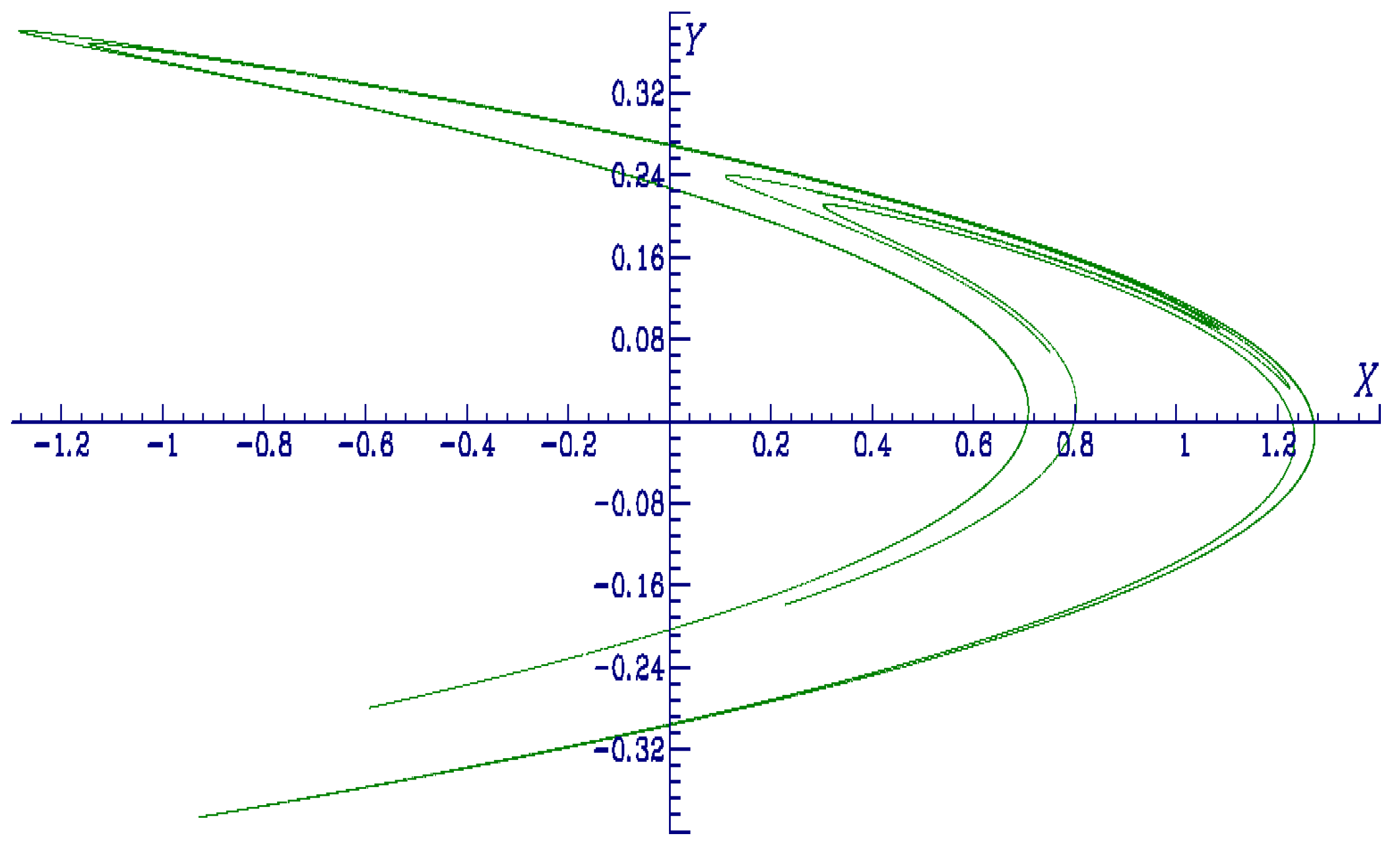
Figure 2.
Original Lozi map in dimension 2 for the parameter value , initial value , .
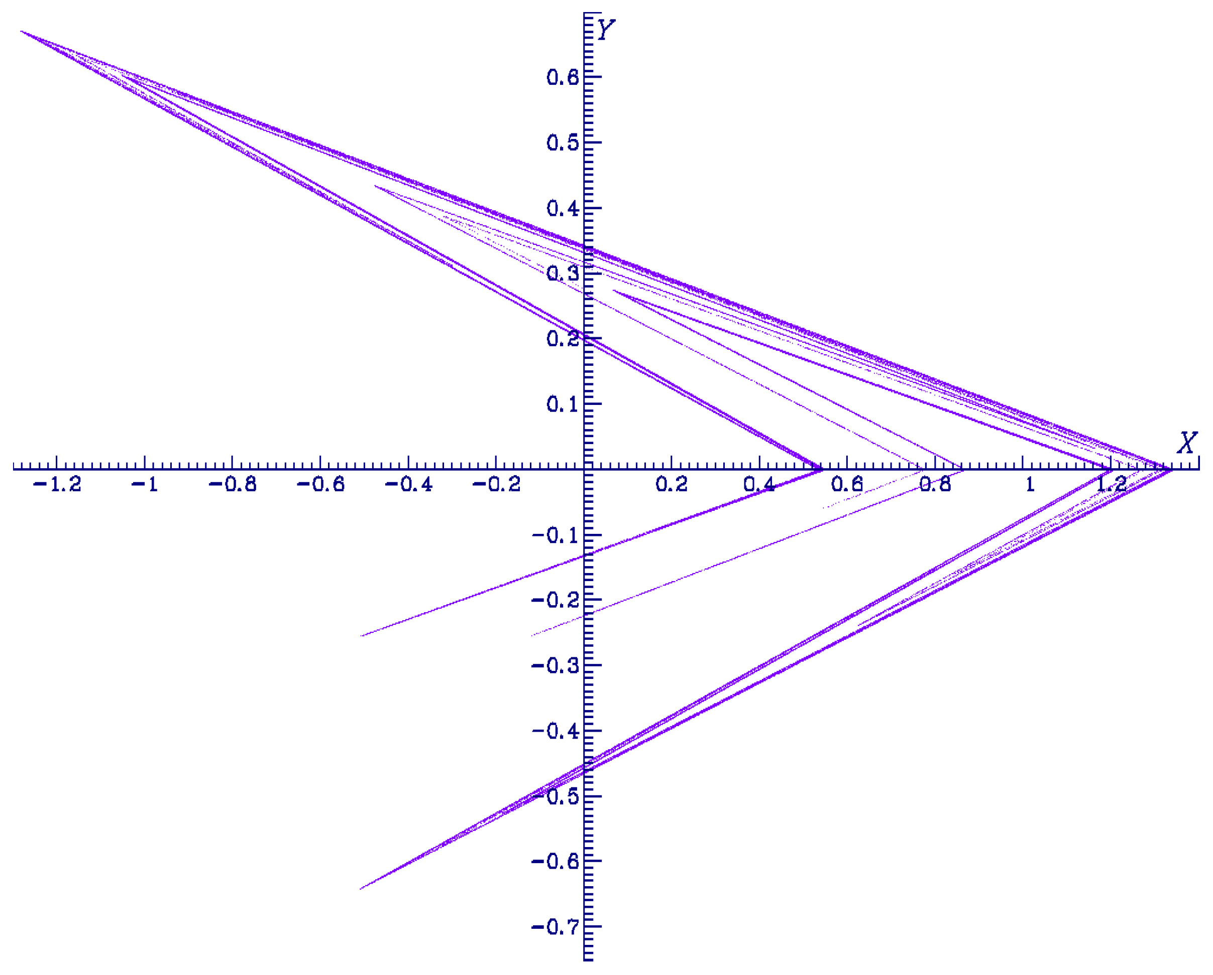
Figure 3.
The set of the plane of parameters where Lozi map has a strange attractor in the first proof of Misiurewicz [8]. Red lines and , blue line , pink line , cyan line , green curve .
Figure 3.
The set of the plane of parameters where Lozi map has a strange attractor in the first proof of Misiurewicz [8]. Red lines and , blue line , pink line , cyan line , green curve .
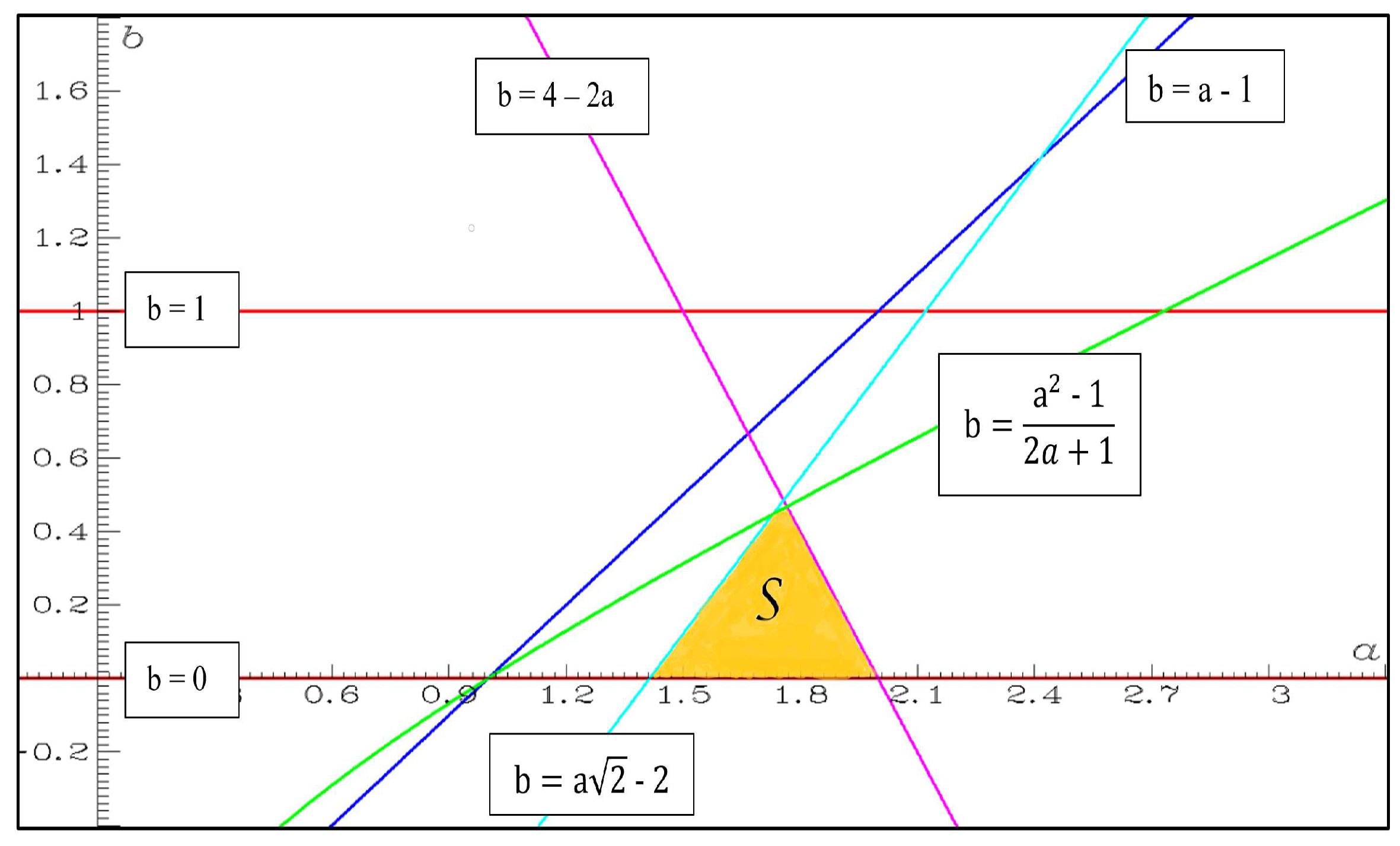
Figure 4.
The sets and of the plane of parameters where Lozi map has a strange attractor in the second proof of Misiurewicz and Stimac [9] and the proof of Kucharski [10]. Blue lines and , cyan lines and , green line , pink line .
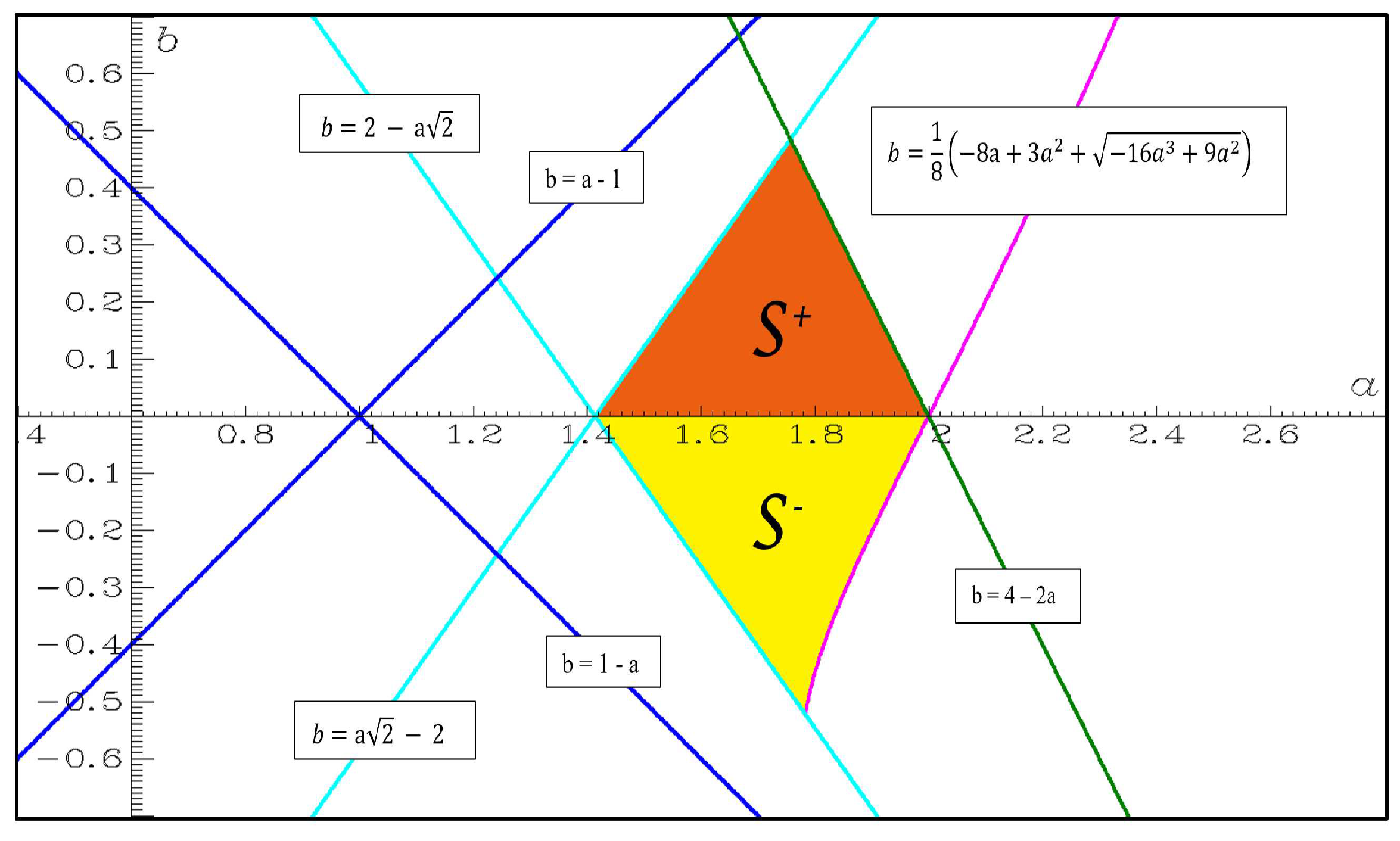
Figure 5.
Periodic, quasi-periodic and chaotic orbits of the area-preserving map (3) in the plane when and . Initial values: red (most extended chaotic orbit) , , dark blue (innermost chaotic orbit inside the red orbit) , , dark green (chaotic orbit inside the red orbit); , (chaotic orbit inside the red orbit); from to upper right corner: brown (periodic orbit) , , brown (periodic orbit) , , brown (periodic orbit) , , brown (periodic orbit) , ; from origin to upper right corner: purple (chaotic orbit) , , magenta (chaotic orbit) , , light green (chaotic orbit) , , light blue (chaotic orbit) , , dark blue (quasiperiodic orbit) , , dark blue (quasiperiodic orbit) , , dark blue (chaotic orbit) , , pink (chaotic orbit) , , green (quasiperiodic orbit) , .
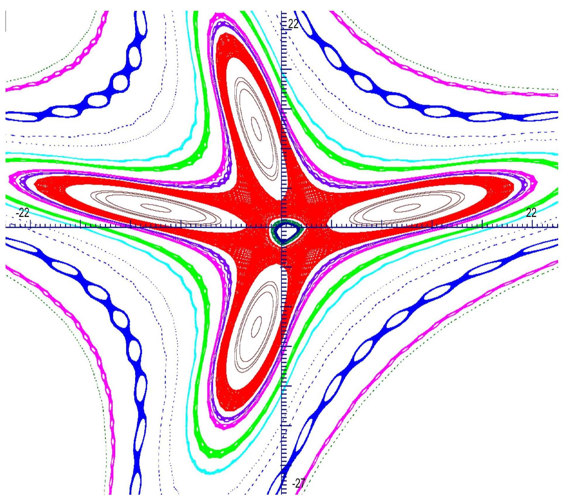
Figure 6.
Image of by a generalized Lozi mapf in the sense of Young [32].
Figure 6.
Image of by a generalized Lozi mapf in the sense of Young [32].
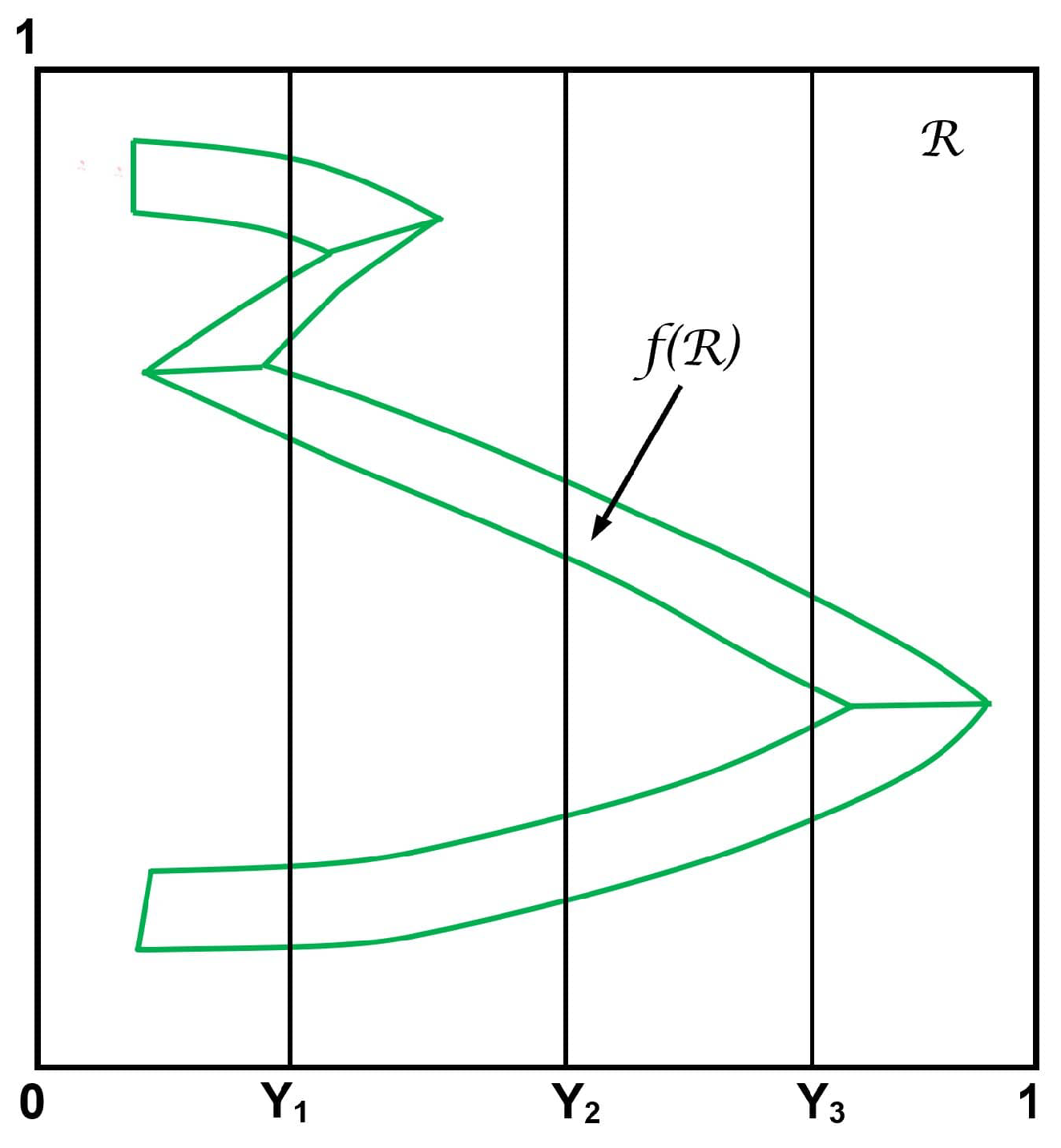
Figure 7.
Image on the -plane of 300,000 iterates of the cosine Lozi chaotic map [44]. Initial value (, .
Figure 7.
Image on the -plane of 300,000 iterates of the cosine Lozi chaotic map [44]. Initial value (, .
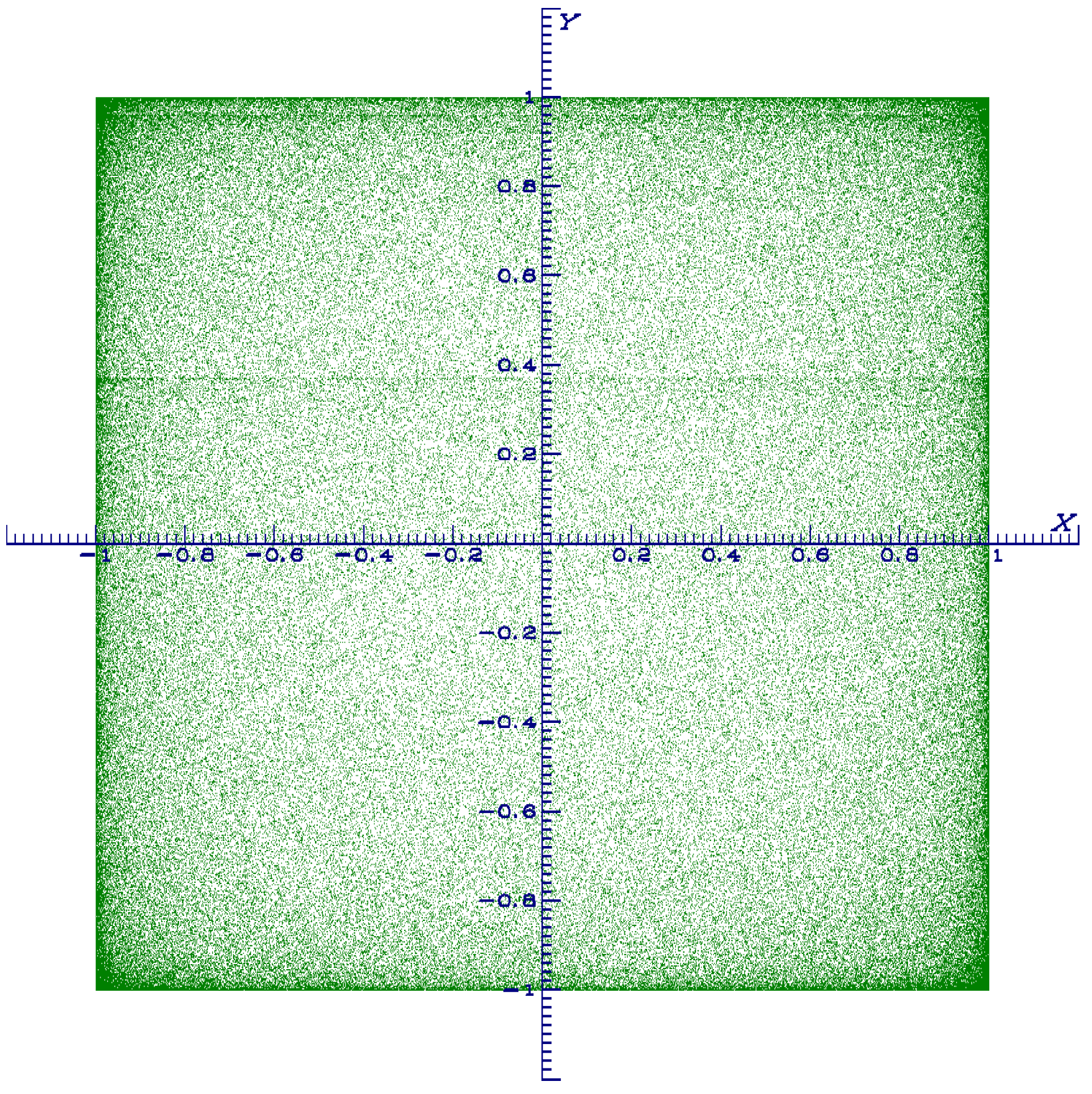
Figure 8.
Projection onto the -plane of the 3-D Ros̎sler "noodle" hyperchaotic attractor. Initial value (, , ).
Figure 8.
Projection onto the -plane of the 3-D Ros̎sler "noodle" hyperchaotic attractor. Initial value (, , ).
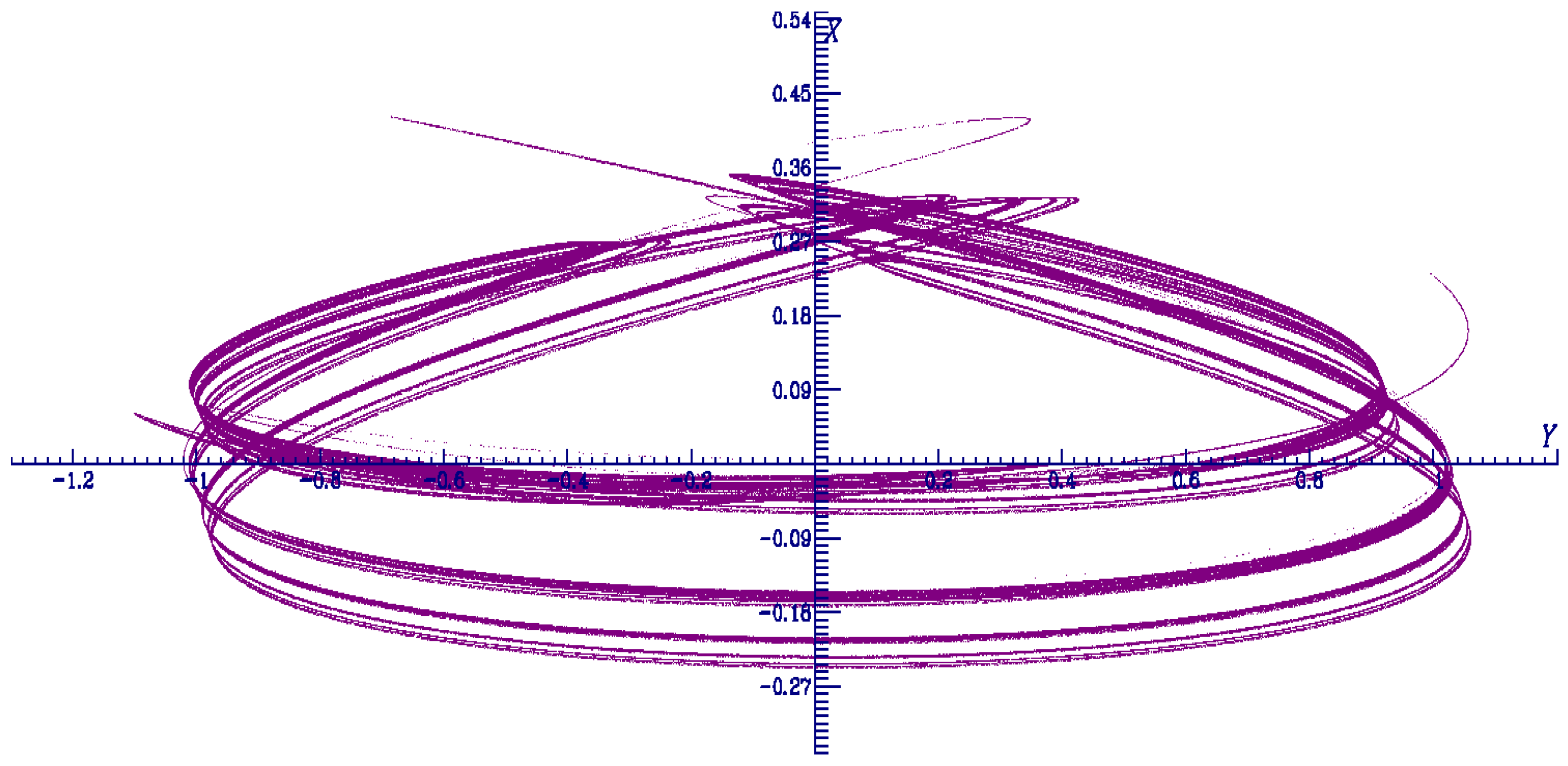
Figure 9.
Projection onto the -plane of the 3-D Rössler "curtain" hyperchaotic attractor. Initial value (, , ).
Figure 9.
Projection onto the -plane of the 3-D Rössler "curtain" hyperchaotic attractor. Initial value (, , ).
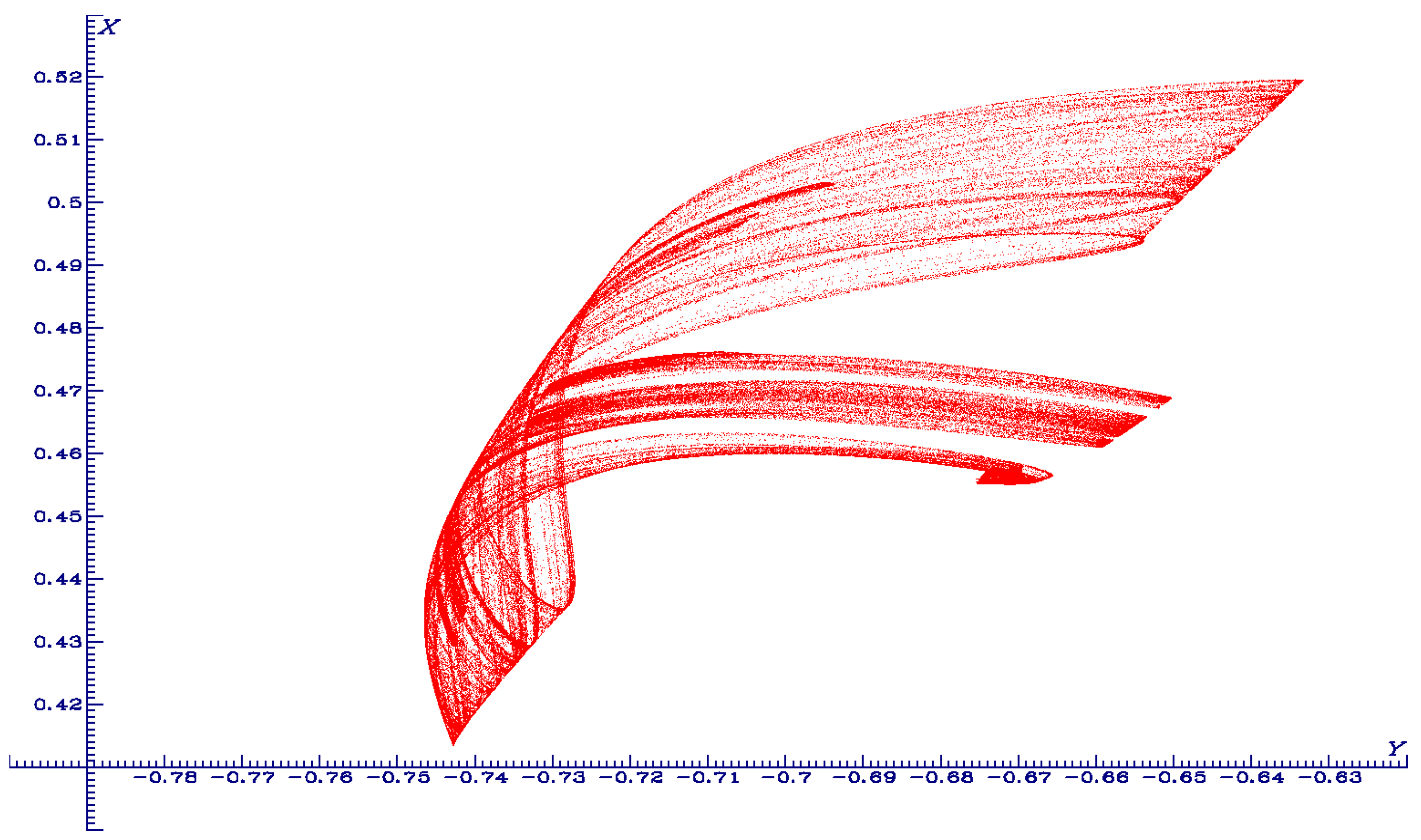
Figure 10.
Projection onto the -plane of the coexisting sheet and thread 3-D Lozi map hyperchaotic attractors for the parameter value . Initial value of the thread-attractor (in green) (, , ). Initial value of the sheet-attractor (in purple) (, , ).
Figure 10.
Projection onto the -plane of the coexisting sheet and thread 3-D Lozi map hyperchaotic attractors for the parameter value . Initial value of the thread-attractor (in green) (, , ). Initial value of the sheet-attractor (in purple) (, , ).
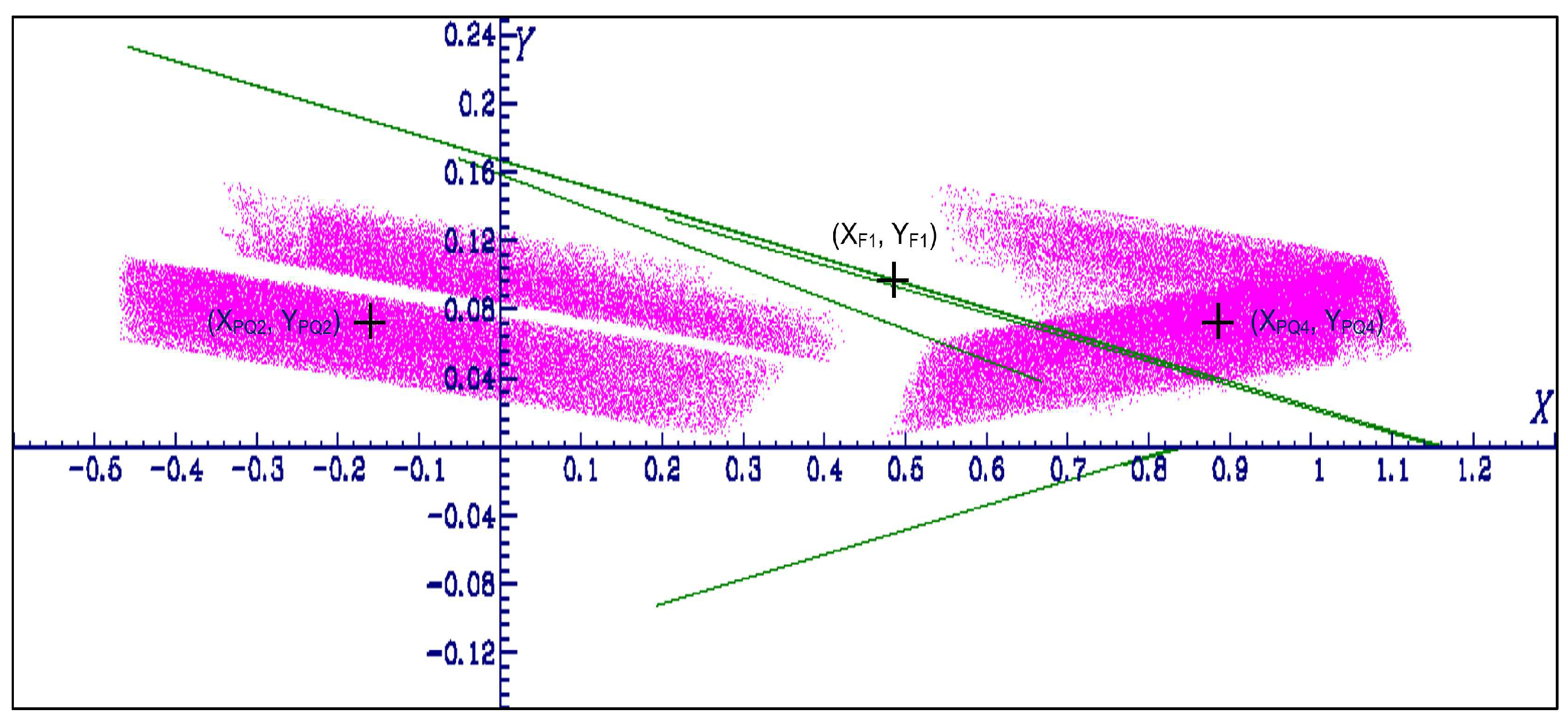
Figure 11.
Projection onto the -plane of the coexisting sheet and thread 3-D Lozi map hyperchaotic attractors for the parameter value . Initial value of the thread-attractor (in green) (, , ). Initial value of the sheet-attractor (in purple) (, , ).
Figure 11.
Projection onto the -plane of the coexisting sheet and thread 3-D Lozi map hyperchaotic attractors for the parameter value . Initial value of the thread-attractor (in green) (, , ). Initial value of the sheet-attractor (in purple) (, , ).
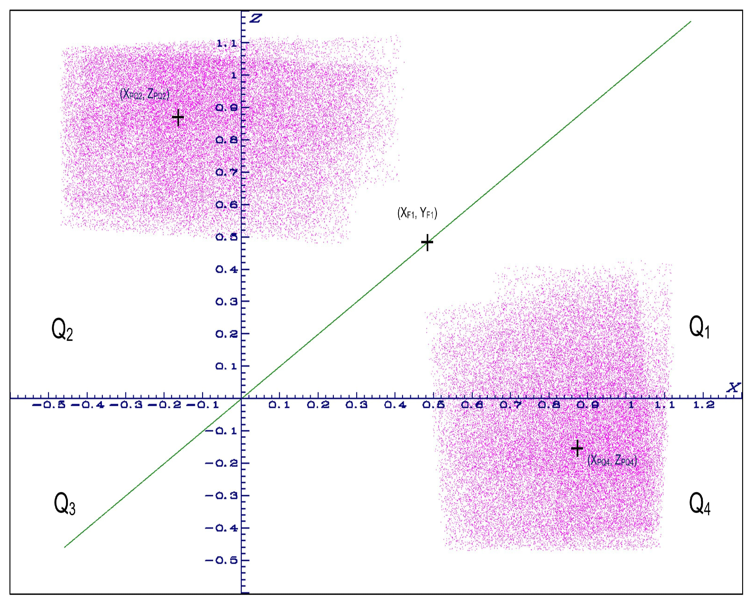
Figure 12.
Projection onto the -plane of the coexisting sheet and thread 3-D Lozi map hyperchaotic attractors for the parameter value , initial value of the thread-attractor (in red) (, , ). Initial value of the sheet-attractor (in cyan) (, , ).
Figure 12.
Projection onto the -plane of the coexisting sheet and thread 3-D Lozi map hyperchaotic attractors for the parameter value , initial value of the thread-attractor (in red) (, , ). Initial value of the sheet-attractor (in cyan) (, , ).
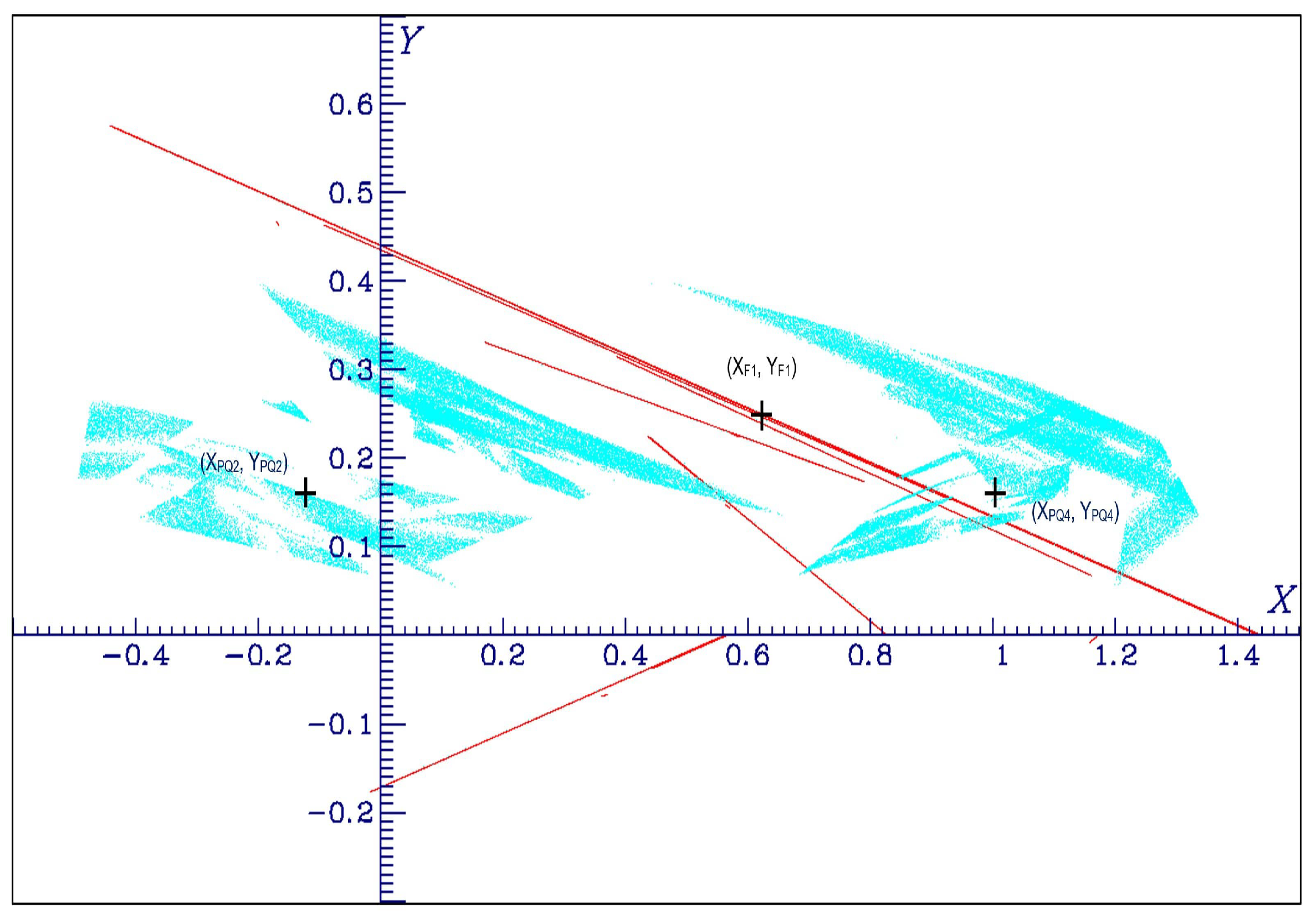
Figure 13.
Projection onto the -plane of the coexisting sheet and thread 3-D Lozi map hyperchaotic attractors for the parameter value , initial value of the thread-attractor (in red) (, , ). Initial value of the sheet-attractor (in cyan) (, , ).
Figure 13.
Projection onto the -plane of the coexisting sheet and thread 3-D Lozi map hyperchaotic attractors for the parameter value , initial value of the thread-attractor (in red) (, , ). Initial value of the sheet-attractor (in cyan) (, , ).
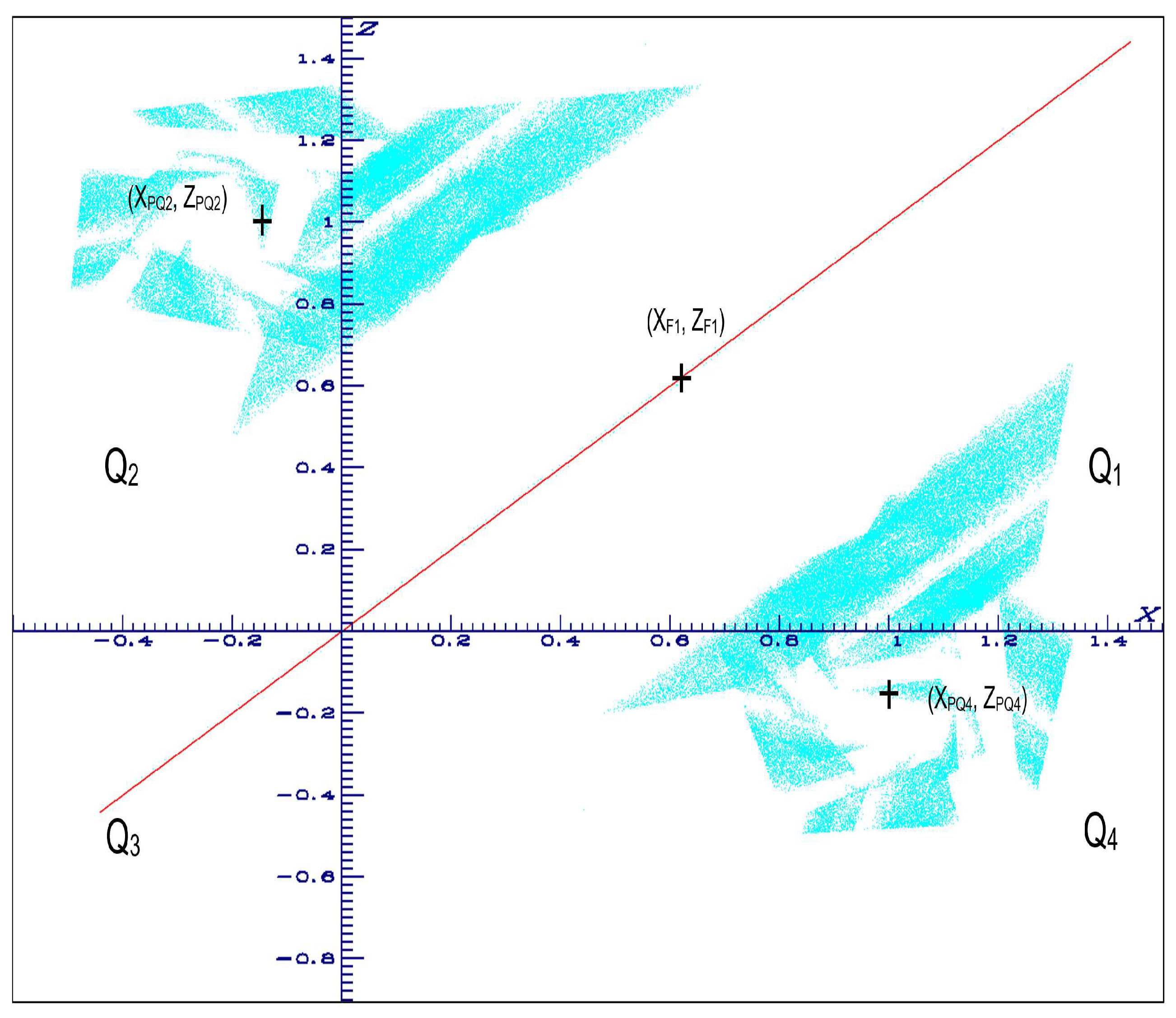
Figure 14.
Magnification of Figure 10 on the -plane of the thread-attractor, showing its fractal structure. Parameter value , initial value of the thread-attractor (, , ).
Figure 14.
Magnification of Figure 10 on the -plane of the thread-attractor, showing its fractal structure. Parameter value , initial value of the thread-attractor (, , ).
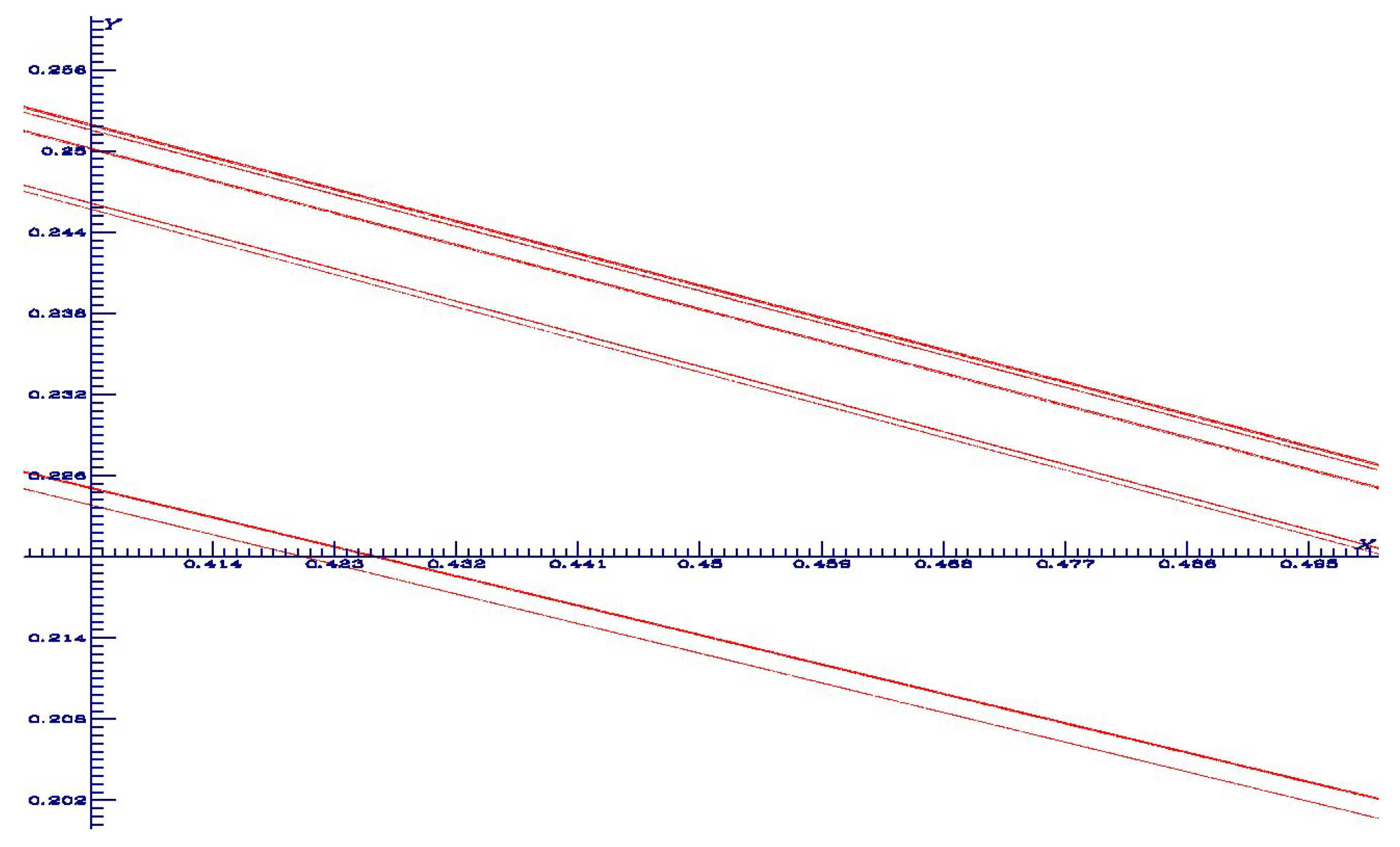
Figure 15.
Projection onto the -plane of the coexisting sheet and thread 3-D Lozi map hyperchaotic attractor for the parameter value . Initial value of the thread-attractor (in purple) (, , ). Initial value of the sheet-attractor (in green) (, , ).
Figure 15.
Projection onto the -plane of the coexisting sheet and thread 3-D Lozi map hyperchaotic attractor for the parameter value . Initial value of the thread-attractor (in purple) (, , ). Initial value of the sheet-attractor (in green) (, , ).
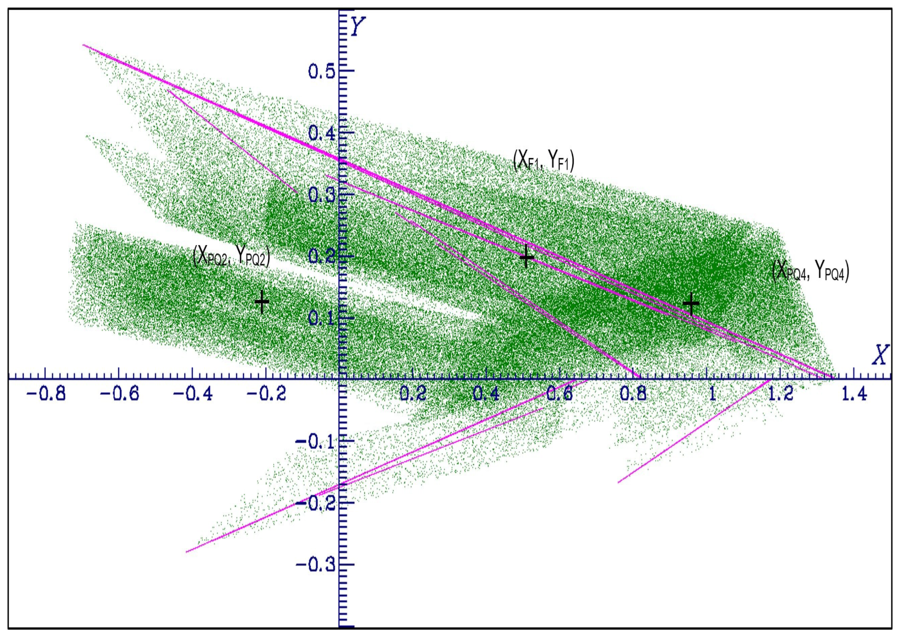
Figure 16.
Projection onto the -plane of the coexisting sheet and thread 3-D Lozi map hyperchaotic attractor for the parameter value . Initial value of the thread-attractor (in purple) (, , ). Initial value of the sheet-attractor (green) (, , ).
Figure 16.
Projection onto the -plane of the coexisting sheet and thread 3-D Lozi map hyperchaotic attractor for the parameter value . Initial value of the thread-attractor (in purple) (, , ). Initial value of the sheet-attractor (green) (, , ).
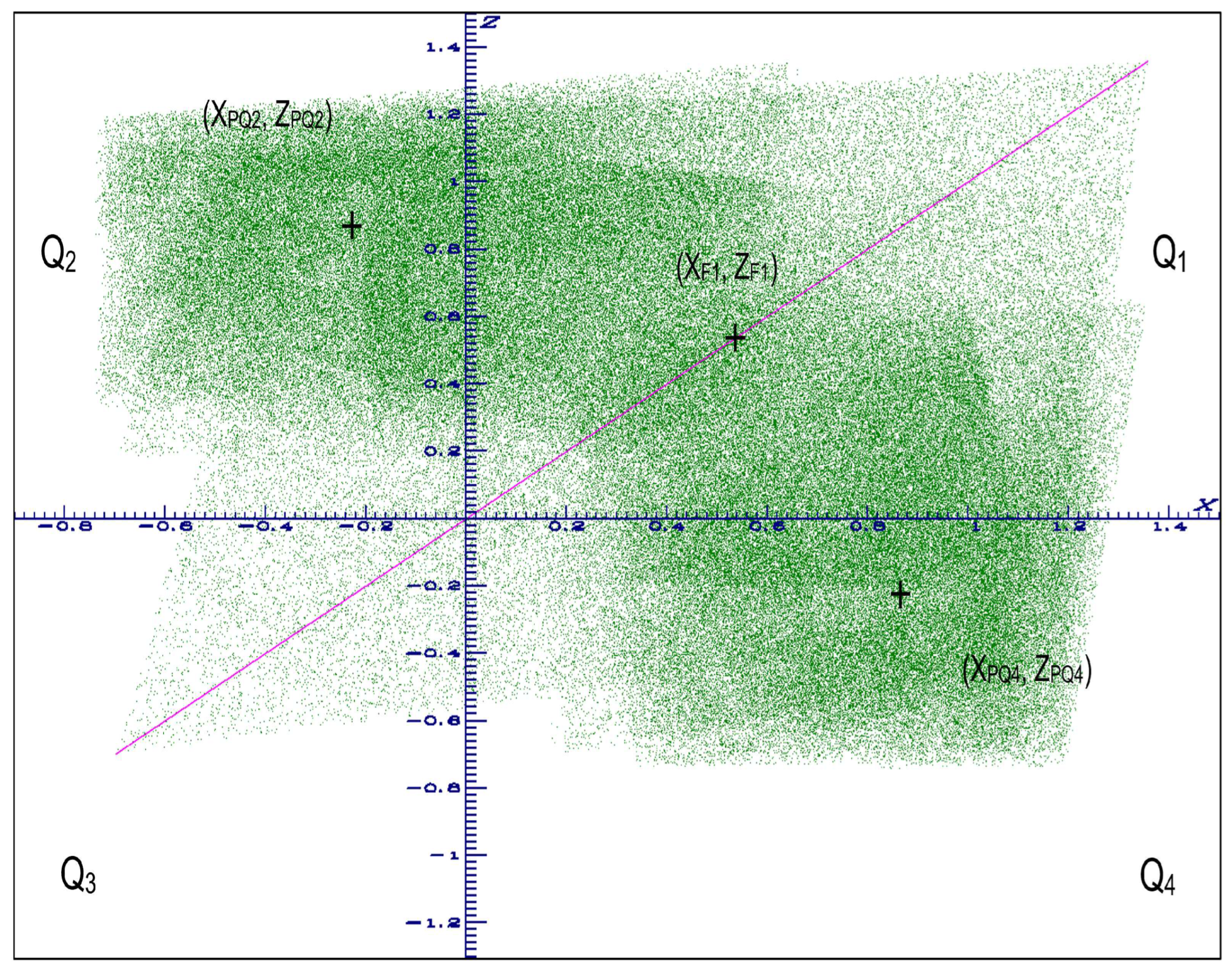
Figure 17.
Projection onto the -plane of two attractors of the 3-D Lozi map chaotic attractor for the parameter values and , . Initial value of both attractors (, , ). When the attractor consists in small red lines (in the three oval regions surrounded by a red curve), instead when there is a blow up of the green attractor which is partially displayed in this magnification of the -phase plane.
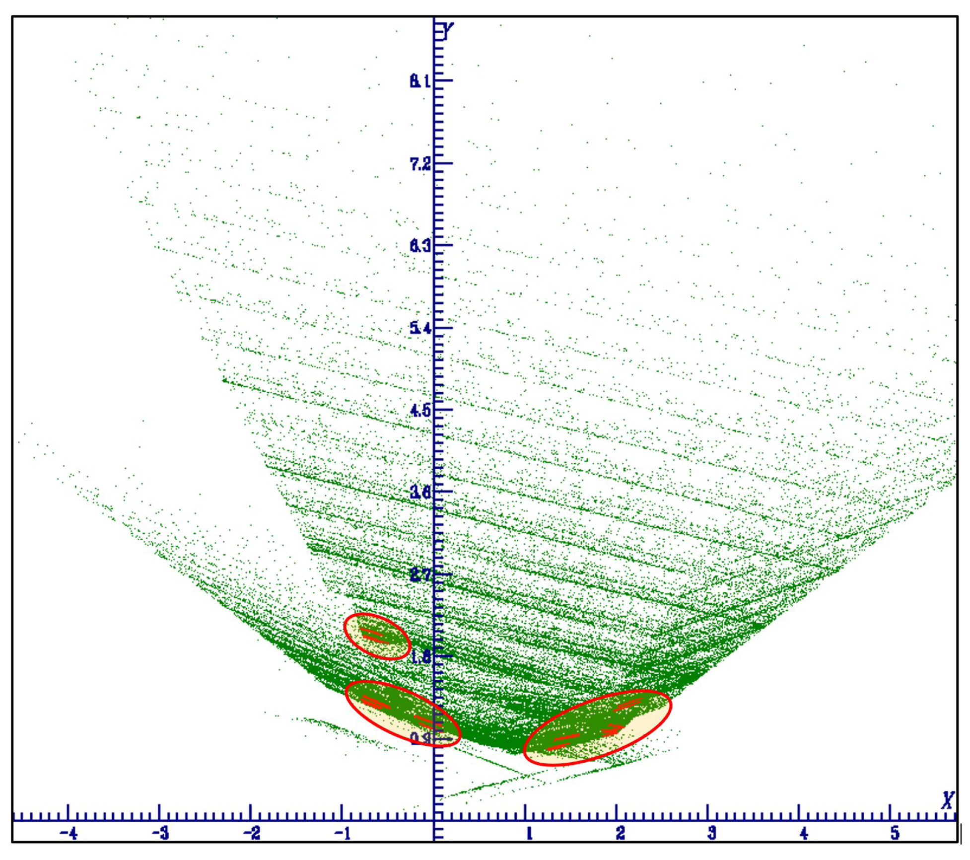
Figure 18.
Projection onto the -plane of two attractors of the 3-D Lozi map chaotic attractor for the parameter values and , . Initial value of both attractors the (, , ). When the attractor consists in small cyan lines (in the four oval regions surrounded by a red curve), instead when there is a blow up of the purple attractor which is partially displayed in this magnification of the -phase plane.
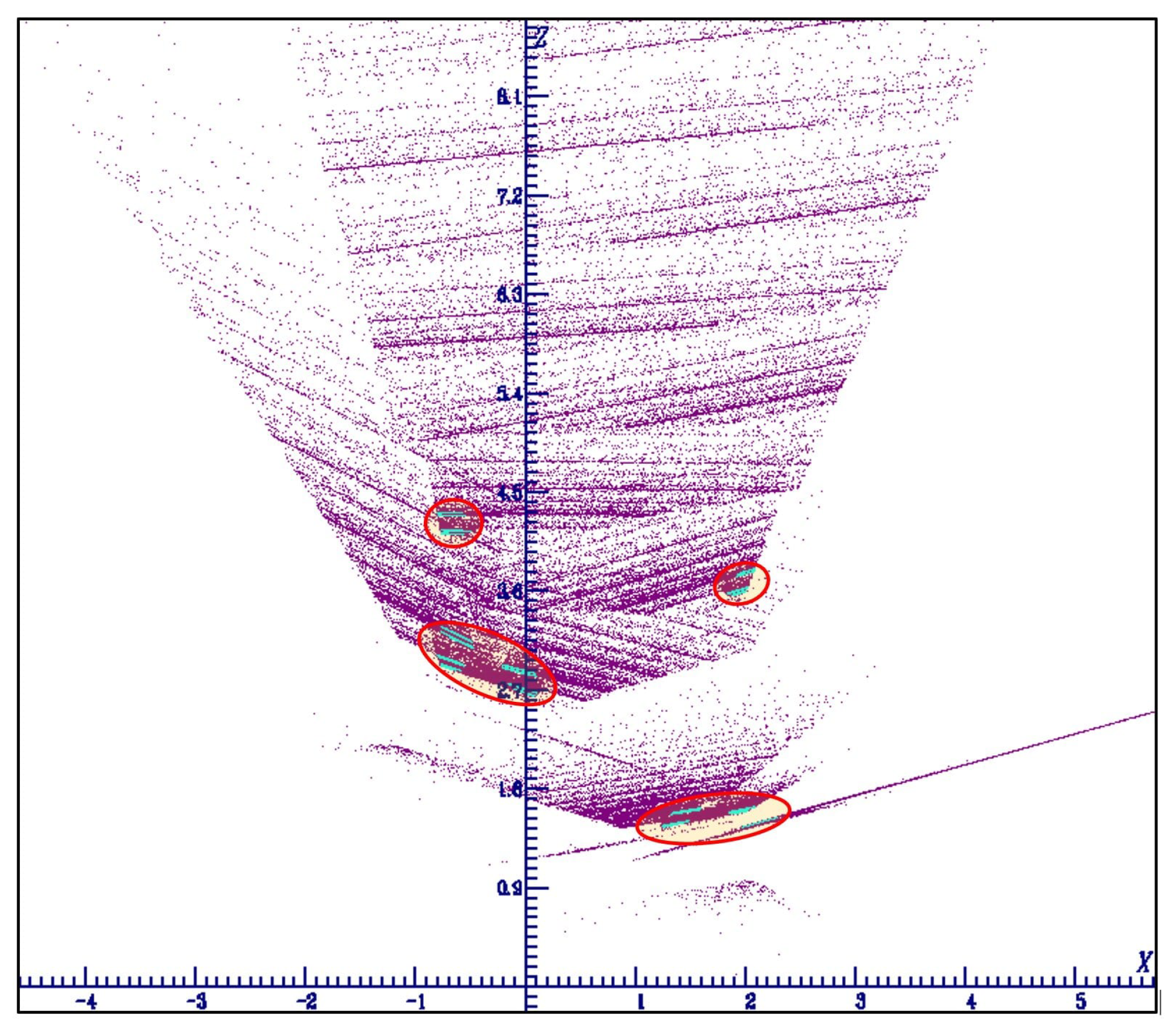
Figure 19.
Projection onto the -plane of two attractors of the 3-D Lozi map chaotic attractor for the parameter values , , (violet), (blue), (purple) and (cyan). Initial value for all attractors (, , ). The attractors for each value of b remain in a small bounded region of the -plane. When b is increased more (see next figure), there is a blowing of the size of the attractor, which remains bounded however.
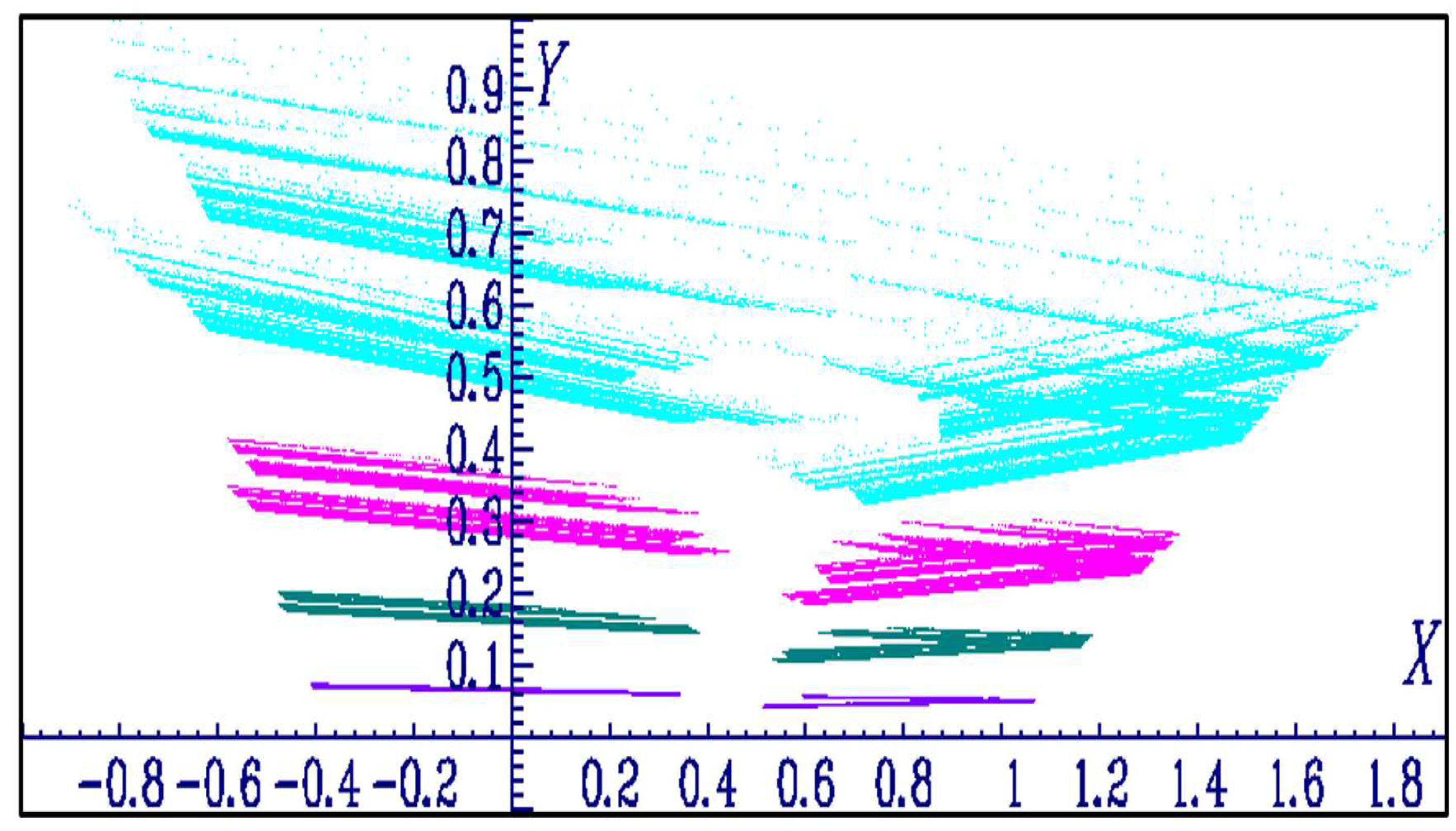
Figure 20.
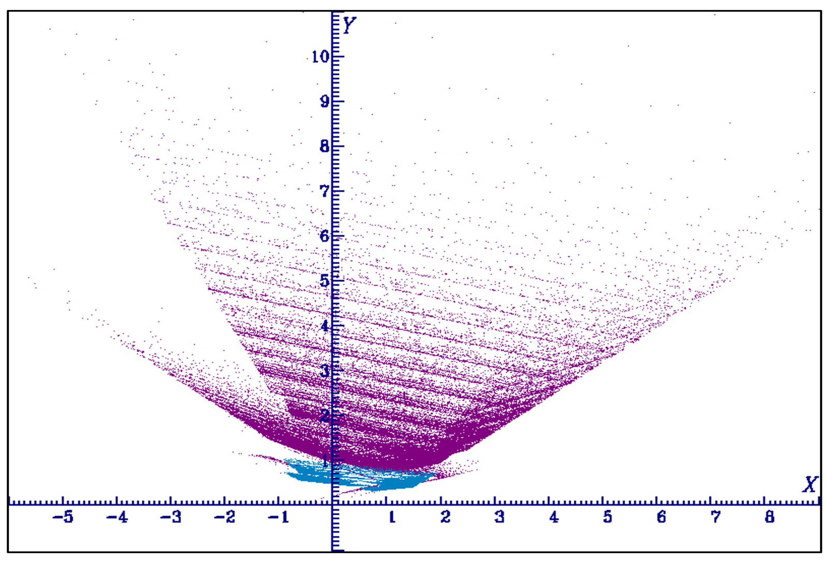
Continuation of the previous figure. Projection onto the -plane of two attractors of the 3-D Lozi map chaotic attractor for the parameter values , , , (cyan) and (purple). Initial value of both attractors (, , ). When the attractor has a small size, instead when there is a blow up of the purple attractor which is partially displayed in this magnification of the -phase plane.
Figure 20.
Continuation of the previous figure. Projection onto the -plane of two attractors of the 3-D Lozi map chaotic attractor for the parameter values , , , (cyan) and (purple). Initial value of both attractors (, , ). When the attractor has a small size, instead when there is a blow up of the purple attractor which is partially displayed in this magnification of the -phase plane.
Disclaimer/Publisher’s Note: The statements, opinions and data contained in all publications are solely those of the individual author(s) and contributor(s) and not of MDPI and/or the editor(s). MDPI and/or the editor(s) disclaim responsibility for any injury to people or property resulting from any ideas, methods, instructions or products referred to in the content. |
© 2023 by the author. Licensee MDPI, Basel, Switzerland. This article is an open access article distributed under the terms and conditions of the Creative Commons Attribution (CC BY) license (http://creativecommons.org/licenses/by/4.0/).
Copyright: This open access article is published under a Creative Commons CC BY 4.0 license, which permit the free download, distribution, and reuse, provided that the author and preprint are cited in any reuse.


