Submitted:
04 February 2024
Posted:
05 February 2024
You are already at the latest version
Abstract
Chaotic theory is commonly being researched for application in image encryption scheme (IES). In this paper, a novel two-dimensional cross hyperchaotic Sine-modulation-Logistic map (2D-CHSLM) based on the famous Sine and Logistic maps. The hyperchaotic behaviors of 2D-CHSLM is testified with the help of their bifurcation diagrams, trajectory plots, Lyapunov exponents, sample entropy, C0 complexity, permutation entropy and 0-1 test. A new bit-level IES with traditional encryption structure is proposed utilizing 2D-CHSLM. The 2D-CHSLM-IES performs a 2D-CHSLM-based bit-level confusion using zig-zag transform and a 2D-CHSLM-based cross coupled diffusion operations for generating a highly secure cipher-image. Then the simulations and security analyses are further carried out with the help of key space, key sensitivity, histogram, correlation, information entropy, differential attack, noise and data loss attacks, prove that the security of the proposed 2D-CHSLM-IES
Keywords:
2D cross hyperchaotic map
; Zig-zag transform
; Cross coupled diffusion
; Bit-level image encryption
1. Introduction
Digital images play a big role in data communication through the networking or any technology, but their security is gradually arousing people’s concern. Multiple image processing approaches were conceived, such as image encryption [1] and watermark [2]. Among them, image encryption scheme (IES) is essential to upholding solitude in image transmitting or safe storage, whether in medicine and military. Employing chaotic theories to enhance the security level of digital images demonstrates strong effectiveness. Chaotic map substantially impact cryptography [3] because it has characteristics of sensitivity to control parameters and initial conditions, pseudo-randomness, ergodicity, and unpredictability [4,5]. It is an effective and practical method to apply chaotic map to IES. Some newly advanced IESs based on chaotic maps using distinct technologies like Josephus traversal [6], deep learning [7], hash functions [8], DNA operation [9], and compression sensing [10] are proposed.
Chaotic maps (CM) are divided into one-dimensional (1D) depicted by difference formulas and high-dimensional (HD) defined by iterative differential formulas. The 1D chaotic map (1D-CM) has simple structure and is easy to implement in computer, which needs less time in the computation process. However, they are many flaws, such as the limited number of parameters and the uneven distribution of their generated state values. In contrast, the HD chaotic map (HD-CM) has more parameters, which can enlarge the range of chaotic behavior. Obviously, HD-CM has more complicated structure and will takes much time. Moreover, for IES, their security is greatly reliant on the performance of the CMs, so it is necessary to construct novel CMs with tremendous chaotic performance. Therefore, the construction of HD-CM is a feasible method to overcome the problems of 1D-CM. Recently, lots of advanced CMs have been designed. Wu et al [11] proposed an IES based on a two-dimensional Logistic map (2D-LM) with complicated basin structures and attractors. In [12], a novel IES based on the newly two-dimensional Sine Logistic modulation map (2D-SLMM) is proposed, which has the large chaotic range and better ergodicity. Sharma [13] designed a novel 2D-CM, which is derived from the idea of giving the two outputs of the 2D-LM to two separate 1D Logistic maps. In [14], Zhu et al defined a 2D Logistic-modulated-sine-coupling-logistic chaotic map (2D-LSMCL), which is a modulation format of the Logistic and Sine maps. A 2D cross-mode hyperchaotic map based on the Logistic and Sine maps (2DCLSS) is presented by Teng et al [15] and then applied to a novel IES.
Since the first chaos-based IES was designed in 1989 [16], many chaos-based IESs have been proposed [17,18,19,20]. Based on Shannon’s information theory, the basic structure of confusion-diffusion is generally adopted [21]. The confusion phase mainly includes two strategies: pixel-level and bit-level permutation. The pixel-level confusion will adjust the pixels’ position while the pixels’ value keeps invariable. However, the bit-level confusion has an advantage that the position and value of a pixel can be changed simultaneously [22]. Hence the bit-level confusion is regarded as more effective [23]. In the diffusion phase, the pixels’ value would be modified. Some bit-level encryption algorithms are being proposed [24,25,26,27].
Motivated by the above analyses, this work introduced a novel bit-level IES by constructing a new 2D cross hyperchaotic Sine-modulation-Logistic map (2D-CHSLM) based on the famous Sine and Logistic maps (2D-CHSLM-IES). 2D-CHSLM-IES consists of three mainly parts, named the initial state calculation, 2D-CHSLM-based bit-level pixel permutation using zig-zag transform, and 2D-CHSLM-based cross coupled pixels diffusion strategy. Simulation tests demonstrate that 2D-CHSLM-IES is superior among the newly advanced IESs and has powerful robustness to the common types of the attacks. The rest of this paper is organized as follows: Section 2 describes and testifies 2D-CHSLM model. Section 3 outlines the related theories of 2D-CHSLM-IES. Section 4 details the newly proposed 2D-CHSLM-IES. The highly security of 2D-CHSLM-IES are analyzed in Section 5. Finally, the conclusions procured from the work are summarized in Section 6.
2. 2D-CHSLM model
This section introduces the proposed 2D-CHSLM and evaluates its hyperchaotic characteristics by comparing it with other existing 2D hyperchaotic maps (2D-HM).
2.1. Definition of 2D-CHSLM
For the common 1D-CMs with limited chaotic range, there is a possibility that the obtained sequences by them may perform weak randomness. It can be substantially avoided by constructing the HD-CM. A 2D-CHSLM is introduced through the cross format in the following. The Logistic map is widely studied traditional 1D-CM because of its complex chaotic behavior, which can be expressed by:
where represents the control parameter and Eq. (1) will enter in chaotic state when . The Sine map is defined as:
where the meanings of the parameters are consistent with Eq. (1). The bifurcation diagram is convenient tool to visualize the chaotic performance of Eq. (1) and Eq. (2). Figure 1 depicts the bifurcation diagram of Eq. (1) and Eq. (2) respectively (Here ). As can be seen in Figure 1, Eq. (1) and Eq. (2) have a small chaotic range, and there are many period windows. This section tries to designed a cross format to enhance their chaotic performance. Consequently, the mathematical formula of 2D-CHSLM is:
where and are the Eq. (2) and Eq. (2) respectively, and the control parameters is . The variables and are obtained values by iterating over the initial variables and .
2.2. Performance evaluation of 2D-CHSLM
To analyze the nonlinearity, complexity, and unpredictability of 2D-CHSLM, several commonly metrics such as bifurcation and trajectory diagram, Lyapunov exponents, sample entropy, C0 complexity, permutation entropy, and 0-1 test are tested. Moreover, this section also compares the hyperchaotic performance of 2D-CHSLM with other advanced 2D-HMs.
2.2.1. Bifurcation diagram
The bifurcation diagram (BD) reflects the advancement of time series as the parameters change. Therefore, BD can be used to measure the nonlinear characteristics of the CM [28,29,30,31]. Figure 2 depicts the BD of 2D-CHSLM with and , and the control parameter within . As shown in Figure 2, 2D-CHSLM has a wide range, and has two iterative sequences that can be randomly distributed in whole space. It means that 2D-CHSLM has a large chaotic range.
2.2.2. Chaos trajectory
Trajectory of the chaotic attractor can directly reflect the nonlinearity and complexity of chaotic maps. For a periodic action, their trajectory is a locked curve. Chaos is bounded, and its trajectory is always limited to a certain range, which is called the chaotic attraction zone. Ideally, the trajectory of chaotic characteristics will not be locked or repeated, and it’s usually occupying a fixed part of the phase space, which can mirror the randomness of the generated chaotic sequence. A large phase space means that the chaotic map can output good random values. When the initial values of 2D-CHSLM are set to , the trajectory diagram is shown in Figure 3. Compared with other 2D-HMs, the trajectory diagram of 2D-CHSLM is more uniformly distributed and extensive. Hence 2D-CHSLM has more complex dynamic characteristics and wider chaotic range.
2.2.3. Lyapunov exponent
For a CM, the Lyapunov exponent () is used to measure the proportion of convergence or divergence of the mean index for two adjacent orbits in phase space [32]. A positive LE value means that adjacent orbits are separated with each iteration, implying the emergence of chaotic state. If the CM has more than one positive LE value, implying the hyperchaotic characteristics. Specifically, a 2D-HM exhibits hyperchaotic characteristics when it has 2 positive LE values. This section firstly adopts the QR decomposition method [33] to analyze whether there is chaotic state in 2D-CHSLM. Its computed process is:
where is the QR decomposition function and represents the Jacobian matrix of the target 2D-HM. Subsequently, the LE of the chaotic map can be solved out via:
Figure 4 depicts the LE value of 2D-CHSLM and the existing 2D chaotic maps (2D-CM) [11,12,13,14,15]. All 2D-CMs depicted from the initial state (, ). Obviously, they exhibit chaotic characteristics. For 2D-CHSLM, their positive values are more than one, proving that there is hyperchaotic state. Specifically, the 2D-LM [11], 2D-SLMM [12], 2D-LALM [13], 2D-LSMCL [14], and 2D-CLSS [15] perform chaotic performance when the control parameter within ( and ), , and,, and (). 2D-CHSLM performs chaotic behaviors when, which has larger chaotic range than other 2D-CMs. Moreover, 2D-SLMM, 2D-LALM, 2D-LSMCL, and 2D CLSS perform hyperchaotic behaviors when the control parameter within , , , and respectively. 2D-CHSLM exhibits hyperchaotic behavior when . It can be concluded that 2D-CHSLM is significantly better than other advanced 2D-CMs and has wider application scenarios.
2.2.4. Sample entropy
Sample entropy (SE) [34] is used to plot the oscillation patterns of time series, which is proportional to the intricacy of the series and can be calculated via:
where , , and are the size of the template vector, the acceptance tolerance, and the length of the time series, and represent the Chebyshev distance between the template vector with and . Generally, a large SE value means that irregular sequences have high complexity. Figure 5 also compare the SE values of 2D-CHSLM with the existing 2D-CMs [11,12,13,14,15], all of which have huge volatilities and even have 0 values, except 2D-CHSLM which the average value is , which is near . It indicated that 2D-CHSLM has better sequence complexity than other 2D-CMs.
2.2.5. C0 complexity
The system complexity is a significant method to analyze their dynamics. The complexity refers to the degree to which series is near random sequence. The bigger the complexity score is, the closer the series is to random series, and the higher the security of applied scheme will be. The complexity of CM can be divided into behavior and structure complexity respectively. Compare to the behavior complexity, the structural complexity, such as C0 method, performs more global statistical significance.
Figure 6 plots the C0 complexity results of 2D-CHSLM and compares with other 2D-CMs. As shown in Figure 6, all 2D-CMs except 2D-SLMM have biased C0s of 0, and the average C0 complexity value of 2D-CHSLM is . It indicated that the complexity of 2D-CHSLM is relatively stable within the parameter range. Prove that the controllability and robustness of the chaotic sequence of 2D-CHSLM.
2.2.6. Permutation entropy
Permutation entropy (PE) [35] is another significant metric used to evaluate the complexity degree of time series. The complexity of chaotic map reflects the degree to which chaotic sequences approach pseudo-random sequences. The higher the complexity result is, the closer the sequence regards as a pseudo-random sequence, and the greater the security is. This section computes the complexity of 2D-CHSLM by their PE value.
Figure 7 plots a equivalence of the PE results of different 2D-CMs [11,12,13,14,15] under parameter swings, half of the 2D-CMs show the value of 0, while the rest illustrate great variation, the mean PE values of 2D-CHSLM is , which testified 2D-CHSLM has superior and more steady sequence intricacy than other 2D-CMs.
2.2.7. 0-1 Test
The 0-1 test is another important metric that evaluates the expansion rates of a nonlinear dynamic map’s series. It can determine the frequency of non-ordinary fixed outcomes of any time series of a 2D-CM. Given a time series for , we execute the following steps,
where is a casual constant, , . Using and , the mean square displacement can be computed via:
subject to,
if the trajectory of and performs the Brownian motion, then expands linearly with time. Otherwise, if the trajectories are bounded, then is bounded. The asymptotic growth proportion of is:
if , proved that the time series performs chaotic characteristics.
For comparative analyses, this section takes sample data , and set the time series obtained by 2D-CHSLM as , . Based on the 0-1 test, the of two time series and are respectively generated. The 2D-CLSS not exhibit chaotic performance when the control parameter near (please see Figure 8a). When , the time series generated by 2D-CLSS performs chaotic behaviors (please see Figure 8b). As shown in Figure 8c, when , the time series generated by 2D-CHSLM doesn’t perform chaotic behaviors. When , of two time series obtained by 2D-CHSLM are near , which is close to 1, the time series enters in hyperchaotic state (please see Figure 8d).
3. Related methods
3.1. Zig-zag transform
The elements in the matrix are sequentially traversed like a “Z” shape, and the traversed elements are sequentially stored in a one-dimensional array, and then transform into a two-dimensional matrix. This whole process is used to permutate the image matrix, named zig-zag transform. It can break the high correlation among image pixels to enhance the security level of IES [36].
Figure 9 depicted a traversed process of the zig-zag transform. For a permutation strategy based on zig-zag transform, the initial position plays a very important roles, different locations may generate different scrambled effects. For example, for a matrix (please see Figure 9a), if the initial position is (1, 1), that means traversing from the first pixel of the matrix, and Figure 9b depicted the matrix after zig-zag transform. This section performs zig-zag transform from the first and the last position of the matrix.
3.2. Cross coupled pixels diffusion strategy
To enhance the diffusion effect, this section proposes a novel diffusion strategy, named cross coupled pixels diffusion (CCPD). In CCPD, the diffusion mechanism proceeds both in the row and column dimension. The diffused values of elements can be determined by their neighboring pixels’ value. Specifically, the columns of the plain-image are dynamically divided into two groups. Then two groups perform CCPD process based on the row and column dimension. For the first group, the diffused values of all elements perform XOR operations via:
where and represent the neighboring column pixel of . Specially, when and , their neighboring columns are and , respectively. means the exclusive-OR operations. is the diffused matrix. Here means the number of rows. For the second group, the diffused values of all elements perform XOR operations via:
where and represent the neighboring row pixel of . Specially, when and , their neighboring columns are and , respectively. is the diffused matrix. Here means the number of columns.
4. The bit-level IES based on 2D-CHSLM
2D-CHSLM can generate highly complex hyperchaotic characteristics with a huge parameter variation. The generated sequence by 2D-CHSLM is uniform, covering the whole phase space. Hence 2D-CHSLM can be applied to IES to enhance its security. Based on 2D-CHSLM, this section further applies 2D-CHSLM to a novel IES, which consists of initial state calculation, 2D-CHSLM-based bit-level pixel permutation using zig-zag transform, and 2D-CHSLM-based coupled pixels diffusion strategy, named 2D-CHSLM-IES. Without loss of generality, the size of the plain-image () used in 2D-CHSLM-IES is .
4.1. Initial state calculation
The key set of 2D-CHSLM-IES mainly consists of three parts, namely the hash value, the random binary array, and parameter key set respectively. The key structure of 2D-HLSM-CECP-IEA has depicted in Figure 11. For the hash value key set, due to the advantage of the hash function is that when making small adjustments to the input, the results are very sensitive and irreversible, making it highly effective against the plaintext attacks, which makes them very suitable for IES, hence the SHA-256 hash function is used to generate the hash value key set in 2D-CHSLM-IES, denoted as . For the random binary array key set, this section randomly generates a binary array with a length of , denoted as . In addition, there are some variables in 2D-CHSLM-IES that serve as secret keys, namely . After initializing the key set , the parameters are obtained and used in 2D-CHSLM to iteratively obtain the chaotic sequence. The detailed steps of are as follows:
Step 1: Input the plain-image into the SHA-256 hash function to generate a hexadecimal number with a length of 64, then convert to decimal and divide it into 8 parts as follows:
Among Eq. (16) and Eq. (17), the function is used to compute the SHA-256 hash value of the input , whereas the function is used to convert a hexadecimal string to their decimal format. refers to the values of from the -th to the -th element.
Step 2: Initialize the random binary array , then divide into 4 sub-parts by converting into the floating-point numbers using the IEEE754 format via Eq. (18):
Step 3: Initialize sub-keystream and use and to adjust the parameters of 2D-CHSLM-IES through Eq. (19):
where is the control parameter of 2D-CHSLM. and are the initial parameter of 2D-CHSLM. means an offset value used in 2D-CHSLM-IES.
Step 4: Set , , and as the parameters of 2D-CHSLM. Input them into of 2D-CHSLM for iteration times and exclude the first values to eliminate the transient effect. Since 2D-CHSLM is 2D, it outputs two iterative series referred to as and , then adjust and via:
4.2. 2D-CHSLM-based bit-level permutation using zig-zag transform
The permutation process comprises two parts: 2D-CHSLM-based bit plane grouping and sorting and 2D-CHSLM-based zig-zag transform. The specific steps are as follows:
Step 1: Read the plain-image and transform into 8 bit-planes, named . Initialize the key set based on Section 4.1.
Step 2: 2D-CHSLM-based bit plane grouping and sorting. Initialize a control sequence for sorting . The index vector is obtained by sorting in ascending order. and are obtained as follows:
where is the sort function, which is used to sort the array and return the sorted array and index vector. To obtain only the index vector , this section can use the “” symbol to ignore the sorted array. Then divide into two groups and as follows:
Step 3: 2D-CHSLM-based zig-zag transform. Perform zig-zag transform on and respectively. For , scanning from the first element. For , scanning from the last element. The specific steps are shown in Section 3.1. The scanned and are saved as and . Then we sort and based on the index vector and . and are obtained as follows:
The sorted and are and . Lastly, divide and into 8 bit-planes, named and merge into a decimal permutated plain-image .
4.3. 2D-CHSLM-based coupled pixel diffusion
The diffusion process comprises two parts: 2D-CHSLM-based dynamical image blocking and 2D-CHSLM-based cross coupled pixels diffusion. The specific steps are as follows:
Step 1: 2D-CHSLM-based dynamical image blocking. Initialize a diffused control sequence for blocking . The index vector is obtained by sorting in ascending order. and are obtained as follows:
Then divide into two groups and based on and via:
Step 2: 2D-CHSLM-based cross coupled pixels diffusion. Select two sub-sequences from as diffused value matrix, named and . and are obtained as follows:
On the one hand, select the columns from and based on , and perform diffused operations using Eq. (14) mentioned in Section 3.2. On the other hand, select the columns from and based on , and perform diffused operations using Eq. (15) mentioned in Section 3.2. Then saved the obtained diffused matrix as the cipher-image .
5. Experimental results and security analyses
To validate the robustness of 2D-CHSLM-IES, this section performs a comprehensive array of experiment and security analysis. The conducted analysis consists of key space analysis, key sensitivity analysis, histogram analysis, correlation coefficient analysis, information entropy analysis, differential attacks analysis, noise and data loss attacks analysis, is executed to assess the efficacy of 2D-CHSLM-IES. The plain-images drawn from the SIPI image databases (https://sipi.usc.edu/database/database.php?volume=misc). These analyses are performed utilizing the MATLAB 2022a running on a compatible computer with Windows 10, 8 GB of RAM, and an Intel(R) CPU Core I5 2.80GHz.
5.1. Visual analysis
To verify the efficiency of the proposed 2D-CHSLM-IES, this section uses several plain-images of different size to stimulate the process. Setting the key stream of 2D-CHSLM-IES. As can be observed from Figure 13, the cipher-images obtained by 2D-CHSLM-IES totally hides the information of their corresponding plain-images, and the decrypted images obtained by 2D-CHSLM-IDS are the same as their original ones. It indicates that the proposed 2D-CHSLM-IES and 2D-CHSLM-IDS can perform the effective security operations of the digital plain-image.
5.2. Key space
A large key space is necessary to withstand the brute force attacks. To enhance the security of IES, the key space should larger than [37]. Suppose the calculation accuracy of 2D-CHSLM-IES is around , thereby the key space of independent keys is respectively. In 2D-CHSLM-IES, it is . The key space of them can be accumulated as follows:
Moreover, SHA-256 is used in 2D-CHSLM-IES to initialize a non-independent hash key set , and a 208-bits is random initialize to be another part of key set. Both and are all used to adjust the original parameters of 2D-CHSLM-IES, and it can be considered that their key space is . whole key space of 2D-CHSLM-IES is larger than , which is far larger than . Hence 2D-CHSLM-IES can make the brute force attacks ineffective.
5.3. Key sensitivity
Key sensitivity indicates that even if there is a tiny modification in key set, IES cannot decode their cipher-image. A tremendous IES must be have high key sensitivity. This section has checked the key sensitivity of 2D-CHSLM-IES. To create a novel key set, a tiny modification is respectively added to the original key set as follows:
Figure14 depicts the key sensitivity results using and on 2D-CHSLM-IES and 2D-CHSLM-IDS. Figure 14d is the pixel-to-pixel differential image of Figure 14b,c. It can be noted from Figure 4 the original image is successfully decoded only by matching key set. Prove that 2D-CHSLM-IES is completely sensitive to key set.
5.4. Histogram
In IES breaking, the usual approach is to find the statistical characteristics of the cipher-image. Those properties can be analyzed by their histogram, which can give expression to the distribution pattern of their gray values. The flatter the histogram distribution is, the less the correlation between the image pixels’ value and the number of pixels, and the more difficult to decode the plain-image information. The histogram tests of 2D-CHSLM-IES and 2D-CHSLM-IDS are shown in Figure 15. As can be observed in Figure 15, the histogram of the plain-image exhibits obvious statistical properties. After 2D-CHSLM-IES is performed, the histogram of the cipher-image is uniformly distributed. In Figure 15, the histogram of the decrypted image obtained by 2D-CHSLM-IDS is the same as their original image.
Moreover, this section further uses the chi-square () test [38] to verify the uniform distribution of the histogram. For a grayscale image of size , supposed the pixel value distribution of each pixel in the histogram is evenly distributed, is the theoretical pixel value distribution, the computed value is , and is the brightness of the grayscale image, and follows the distribution of with 255 degrees of freedom:
When , it means the value passes the test. The calculation results tabulated in Table 1 illustrated the computed test results of the cipher-images, which indicates that the gray distribution of the cipher-image is uniform.
In addition, this section analyzes the histogram of cipher-images via their variance [39]:
where represents the gray value, and and are the number of pixels whose gray value is and respectively. When the variance of the histogram is smaller, the pixel distribution is more uniform, and the ability to withstand the statistical attacks is greater.
Table 2 tabulates the variance value of the cipher-image obtained by 2D-CHSLM-IES. It can be observed that the variance values are less than , indicating that the average fluctuation of number of pixels in each gray value is less than , which can more effectively withstand the statistical attacks. Table 3 further illustrates the percentage of the variance differences to analyze the effect of changing the key sets on the uniformity of the cipher-image. For , the average variance fluctuation is . A tiny modification on will obtain the biggest variance fluctuating value , while the smallest one is by changing . Those results demonstrate that 2D-CHSLM-IES can withstand the statistical attacks.
5.5. Correlation
It is another statistical analysis method that is used to find the relationship between adjacent pixels of one image, which may be exploited by the attackers. Hence the IES should have the ability of improving the security of the digital image data by breaking the correlation between their neighboring pixels. To test the security of 2D-CHSLM-IES, this section computes the magnitude of the correlation coefficient between neighboring pixels in horizontal (H), vertical (V), and diagonal (D) directions by the randomly 10000-pixel’ value of the image via [40]:
where and represent pixel values of two neighboring pixels, is the chosen number of pixels. is the covariance of and . and is the variance and expectation, respectively. When close to 1, it means a high correlation, otherwise, a low correlation.
Table 4 illustrates the correlation coefficient results of the different plain-images and the corresponding cipher-images for all three directions. As can be observed in Table 4, the correlation between the pixel value is high in the case of plain-images whereas the correlation of the cipher-image is near 0. Moreover, Table 4 compares the correlation coefficient results with Ref. [41]. Obviously, 2D-CHSLM-IES has a lower correlation than those IESs in all three directions. It implies that 2D-CHSLM-IES is highly resist the statistical attacks.
Figure 16 depicts the correlation coefficient of the plain-image “5.1.12” and their corresponding cipher-image. As can be seen, the correlation coefficient results are scattered around a straight line which indicates a high correlation for all three directions. On the contrary, the correlation coefficient results of the cipher-image are scattered evenly on the plane which indicates that the image information has extremely low relationships among them after 2D-CHSLM-IES operations.
5.6. Information entropy
Information entropy is another metric of the statistical analysis. It is used to quantitatively analyze the randomness of the image data. The higher the information entropy, the higher the usable data, a good IES should process the image with an information entropy near 0. The entropy can be calculated via:
where is the number of gray levels present in an image, while is the probability of a specific gray level occurring in the image. For a grayscale image (), their ideal value of is 8. Thus, the cipher-image with a near 8 means greater randomness and better effect. Table 5 tabulates the computed of different plaint-images and the cipher-images using 2D-CHSLM-IES. Moreover, Table 5 also compare the computed with other IESs [41,42,43]. The results imply that 2D-CHSLM-IES performs tremendous encryption performance.
5.7. Differential attack
Similar to Section 5.3, the differential attack is a way to analyze the sensitivity of one IES. In this attack, the hacker tries to find the statistical patterns of an image. There are two commonly metrics to measure the ability of an IES against the differential attacks, Number of Pixels Change Rate () and Unified Average Changing Intensity (). The numerical equations are as follows:
Among Eq. (35) and Eq. (36), and are the rows and columns of an image, respectively. and represent two cipher-images which their original images have only one pixel value that is slightly different. The theoretical values are and , respectively.
Moreover, the acceptable intervals for and are given in the REF at the significance [44]:
where when , , and . Table 6 tabulates the ranges of and for images of different sizes.
Table 7 tabulates the obtained NPCR and UACI scores for different images and compare them with other IESs. Obviously, all scores are totally near their theoretical scores than all other methods. Also, the obtained scores of NPCR and UACI have been analyzed for significance value at α = 0.05 [44]. It is not hard to find that 2D-CHSLM-IES passes the tests, which indicates the ability of 2D-CHSLM-IES against the differential attacks.
5.8. Noise and data loss attacks
Robustness is a significant metric to measure the anti-interference ability of an IES. This section verifies the robustness of 2D-CHSLM-IES against the two common corruption sources, noise attack and data loss attack respectively.
5.8.1. Robust to noise attacks
Noise attack is a common corruption source during transmission. An effective IES must be roust to this kind types of attacks. The mainly noises include speckle noise, pepper and salt noise, etc. This section analyzes the effect of adding those two noises to the cipher-image “gray21.512”. On the premise that the key set remains unchanged, different intensities of the pepper and salt noise are added to the cipher- image. Then 2D-CHSLM-IDS is used to decode these cipher-images. Figure 17 depicts the cipher-images with different noise intensities (0.01, 0.05, 0.0001, and 0.0005) and their corresponding decoded images by 2D-CHSLM-IDS. As shown in Figure 17, even if the noise intensity reaches 0.05 and 0.0005, we can still recognize their original image. Hence 2D-CHSLM-IES is effective to the noise attacks.
5.8.2. Robust to data loss attacks
Data loss attack is another common corruption source during transmission. An effective IES must be roust to this kind types of attacks. The usual approach is to assume that the cipher-image has lost different proportions of data, and then use IES to try to decode their corresponding original image. Obviously, as the proportion of data loss increases, the quality of the decrypted image gradually decreases. Figure 18 depicts the cipher-images “5.3.01” with different proportions (, , and ) of data loss and their corresponding decoded images. As shown in Figure 18, the main information can still recognize from their decoded image. Hence 2D-CHSLM-IES is effective to the data loss attacks. It means that 2D-CHSLM-IES is robust to noise and data loss attacks.
6. Conclusion
In this paper, a new bit-level IES based on 2D-CHSLM is designed, which uses Zig-zag transforms and cross coupled diffusion strategy to enhance security. 2D-CHSLM performs complex hyperchaotic characteristics and is highly suitable for application in IES, which are verified by their BD and trajectory diagrams, LE, SE, C0s and PE, and 0-1 test respectively. The chaotic sequence generated by 2D-CHSLM is used to encrypt the plain-image, which largely improves the key sensitivity of 2D-CHSLM-IES. 2D-CHSLM-based bit-level confusion using Zig-zag transform and 2D-CHSLM-based cross coupled diffusion strategy can further enhance the security level. The proposed 2D-CHSLM-IES is robust to the common types of attacks, such as the brute force attacks, statistical attacks, differential attacks, noise and data loss attacks, and its comprehensive performance is superior than other advanced IESs.
Acknowledgements
This work is supported by the National Natural Science Foundation of China (Nos: 62176037 and 61701070), the Fundamental Research Funds for the Central Universities (Nos:3132023252), China Postdoctoral Science Foundation (No: 2020M680933).
References
- Liu, H.; Liu, J.; Ma, C. Constructing dynamic strong S-Box using 3D chaotic map and application to image encryption. Multimed Tools Appl. 2023, 82, 23899–23914. [Google Scholar] [CrossRef]
- Xia, Z.; Wang, X.; Zhou, W.; Li, R.; Wang, C.; Zhang, C. Color medical image lossless watermarking using chaotic system and accurate quaternion polar harmonic transforms. Signal Process. 2019, 157, 108–118. [Google Scholar] [CrossRef]
- Wei, Z. Dynamical behaviors of a chaotic system with no equilibria. Phys Lett A 2011, 376, 102–108. [Google Scholar] [CrossRef]
- Peng, H.-H.; Xu, X.-M.; Yang, B.-C.; Yin, L.-Z. Implication of two-coupled differential Van der Pol duffing oscillator in weak signal detection. J Phys Soc Jpn 2016, 85, 044005. [Google Scholar] [CrossRef]
- Boriga, R.; Dascalescu, A.C.; Priescu, I. A new hyperchaotic map and its application in an image encryption scheme. Signal Process: Image Commun 2014, 29, 887–901. [Google Scholar] [CrossRef]
- Wang, M.; Wang, X.; Wang, C.; Zhou, S.; Xia, Z.; Li, Q. Color image encryption based on 2D enhanced hyperchaotic logistic-sine map and two-way Josephus traversing. Digit. Signal Process. 2023, 132, 103818. [Google Scholar] [CrossRef]
- Alsubaei, F.S.; Alneil, A.A.; Mohamed, A.; Hilal, A.M. Block-Scrambling-Based Encryption with Deep-Learning-Driven Remote Sensing Image Classification. Remote Sens. 2023, 15, 1022. [Google Scholar] [CrossRef]
- Hu, Y.; Nan, L. Image encryption algorithm based on 1D-SFACF with cross-cyclic shift and adaptive diffusion. Phys Scr. 2023, 98, 055209. [Google Scholar] [CrossRef]
- Yan, X.; Wang, X.; Xian, Y. Chaotic image encryption algorithm based on arithmetic sequence scrambling model and DNA encoding operation. Multimed Tools Appl. 2022, 80, 10949–10983. [Google Scholar] [CrossRef]
- Wang, M.; Wang, X.; Wang, C.; Xia, Z.; Zhou, S. Novel Image Compression-Then-Encryption Scheme Based on 2D Cross Coupled Map Lattice and Compressive Sensing. Multimed Tools Appl. 2023, 83, 1891–1917. [Google Scholar] [CrossRef]
- Wu, Y.; Yang, G.; Jin, H.; Noonan, J.P. Image encryption using the two-dimensional logistic chaotic map. J Electron Imaging. 2012, 21, 013014. [Google Scholar] [CrossRef]
- Hua, Z.; Zhou, Y.; Pun, C.M.; Chen, C. 2D Sine Logistic modulation map for image encryption. Inf Sci. 2014, 297, 80–94. [Google Scholar] [CrossRef]
- Sharma, M. Image encryption based on a new 2D logistic adjusted logistic map. Multimed. Tools Appl. 2020, 79, 355–374. [Google Scholar] [CrossRef]
- Zhu, H.; Zhao, Y.; Song, Y. 2D Logistic-Modulated-Sine-Coupling-Logistic Chaotic Map for Image Encryption. IEEE Access 2019, 7, 14081–14098. [Google Scholar] [CrossRef]
- Teng, L.; Wang, X.; Xian, Y. Image encryption algorithm based on 2D-CLSS hyperchaotic map using simultaneous permutation and diffusion. Inf Sci. 2022, 605, 71–85. [Google Scholar] [CrossRef]
- Matthews, R. On the derivation of a chaotic encryption algorithm. Cryptologia 1989, 13, 29–42. [Google Scholar] [CrossRef]
- Wang, M.; Wang, X.; Zhao, T.; Zhang, C.; Xia, Z.; Yao, N. Spatiotemporal chaos in improved Cross Coupled Map Lattice and its application in a bit-level image encryption scheme. Inf Sci. 2021, 544, 1–24. [Google Scholar] [CrossRef]
- Zhang, Z.; Tang, J.; Ni, H.; Huang, T. Image adaptive encryption algorithm using a novel 2D chaotic system. Nonlinear Dyn. 2023, 111, 10629–10652. [Google Scholar] [CrossRef]
- Zhou, S.; Zhao, Z.; Wang, X. Novel chaotic colour image cryptosystem with deep learning. Chaos Soliton Fract. 2022, 161, 112380. [Google Scholar] [CrossRef]
- Lai, Q.; Liu, Y. A cross-channel color image encryption algorithm using two-dimensional hyperchaotic map. Expert Syst Appl. 2023, 223, 119923. [Google Scholar] [CrossRef]
- Peng, F.; Zhang, X.; Lin, Z.; Long, M. A tunable selective encryption scheme for H.265/HEVC based on chroma IPM and coefficient scrambling. IEEE Trans Circuits Syst Video Technol 2020, 30, 2765–2780. [Google Scholar] [CrossRef]
- Wu, Y.; Zhou, Y.; Saveriades, G.; Agaian, S.; Noonan, J.P.; Natarajan, P. Local Shannon entropy measure with statistical tests for image randomness. Inf Sci. 2022, 222, 323–342. [Google Scholar] [CrossRef]
- Tang, Z.; Song, J.; Zhang, X.; Sun, R. Multiple-image encryption with bit-plane decomposition and chaotic maps. Opt Lasers Eng. 2016, 80, 1–11. [Google Scholar] [CrossRef]
- Wang, M.; Wang, X.; Wang, C.; Xia, Z.; Zhao, H.; Gao, S.; Zhou, S.; Yao, N. Spatiotemporal chaos in cross coupled map lattice with dynamic coupling coefficient and its application in bit-level color image encryption. Chaos Soliton Fract. 2020, 139, 110028. [Google Scholar] [CrossRef]
- Wang, M.; Liu, H.; Zhao, M. Bit-level image encryption algorithm based on random-time S-Box substitution. Eur. Phys. J. Spec. Top. 2022, 231, 3225–3237. [Google Scholar] [CrossRef]
- Li, J.; Wang, J.; Di, X. Image encryption algorithm based on bit-level permutation and "Feistel-like network" diffusion. Multimed Tools Appl. 2022, 81, 44335–44362. [Google Scholar] [CrossRef]
- Devipriya, M.; Brindha, M. Image encryption using modified perfect shuffle-based bit level permutation and learning with errors based diffusion for IoT. Comput Electr Eng, 2022, 100, 107954. [Google Scholar]
- Luo, J.; Xu, X.; Ding, Y.; Yuan, Y.; Yang, B.; Sun, K.; Yin, L. Application of a memristor-based oscillator to weak signal detection. Eur. Phys. J. Plus, 2018, 133, 239. [Google Scholar] [CrossRef]
- ul Haq, T.; Shah, T. 4D mixed chaotic system and its application to RGB image encryption using substitution diffusion. J Inf Secur Appl, 2021, 61, 102931. [Google Scholar] [CrossRef]
- Wang, X.; Guan, N. 2D sine-logistic-tent-coupling map for image encryption. J. Ambient. Intell. Humaniz. Comput, 2022, 14, 13399–13419. [Google Scholar] [CrossRef]
- Wang, X.; Guan, N.; Yang, J. Image encryption algorithm with random scrambling based on one-dimensional logistic self-embedding chaotic map. Chaos Soliton Fract. 2021, 150, 111117. [Google Scholar] [CrossRef]
- Li, Y.; Li, C.; Liu, S.; Hua, Z.; Jiang, H. A 2-D conditional symmetric hyperchaotic map with complete control. Nonlinear Dyn. 2022, 109, 1155–1165. [Google Scholar] [CrossRef]
- Hu, X.; Jiang, D.; Ahmad, M.; Tsafack, N.; Zhu, L.; Zheng, M. Novel 3-D hyperchaotic map with hidden attractor and its application in meaningful image encryption. Nonlinear Dyn. 2023, 111, 19487–19512. [Google Scholar] [CrossRef]
- Richman, J.; Moorman, J. Physiological time-series analysis using approximate entropy and sample entropy. American Journal of Physiology-Heart and Circulatory Physiology, 2000, 278, H2039–H2049. [Google Scholar] [CrossRef] [PubMed]
- Gao, X. Image encryption algorithm based on 2D hyperchaotic map. Opt. Laser Technol. 2021, 142, 107252. [Google Scholar] [CrossRef]
- Huo, D.; Zhu, Z.; Wei, L.; Han, C.; Zhou, X. A visually secure image encryption scheme based on compressive sensing. Opt. Commun. 2021, 492, 126976. [Google Scholar] [CrossRef]
- Mao, N.; Tong, X.; Zhang, M.; Wang, Z. Real-time image encryption algorithm based on combined chaotic map and optimized lifting wavelet transform. :J Real-Time Image Pr. 2023, 20, 35. [Google Scholar] [CrossRef]
- Cao, C.; Sun, K.; Liu, W. A novel bit-level image encryption algorithm based on 2D-LICM hyperchaotic map. Signal Process. 2018, 143, 122–133. [Google Scholar] [CrossRef]
- Parida, P.; Pradhan Pradhan, C.; Gao, X.; Roy, D.S.; Barik, R.K. Image encryption and authentication with elliptic curve cryptography and multidimensional chaotic maps. IEEE Access, 2021, 9, 76191–76204. [Google Scholar] [CrossRef]
- Wang, M.; Wang, X.; Zhang, Y.; Zhou, S.; Zhao, T.; Yao, N. A novel chaotic system and its application in a color image cryptosystem. Opt Lasers Eng. 2019, 121, 479–494. [Google Scholar] [CrossRef]
- Wang, X.; Chen, X.; Zhao, M. A new two-dimensional sine-coupled-logistic map and its application in image encryption. Multimed Tools Appl. 2023, 82, 35719–35755. [Google Scholar] [CrossRef]
- Wang, X.; Zhao, M. A new spatiotemporal chaos model and its application in bit-level image encryption. Multimed Tools Appl. 2023, 83, 10481–10502. [Google Scholar] [CrossRef]
- Liang, Q.; Zhu, C. A new one-dimensional chaotic map for image encryption scheme based on random DNA coding. Opt. Laser Technol. 2023, 160, 109033. [Google Scholar] [CrossRef]
- Wu, Y.; Noonan, J.P.; Agaian, S. NPCR and UACI randomness tests for image encryption. Cyber J. Multidiscipl. J. Sci. Technol. J. Sel. Areas Telecommun. 2011, 1, 31–38. [Google Scholar]
Figure 2.
BD of 2D-CHSLM: (a) and (b) .
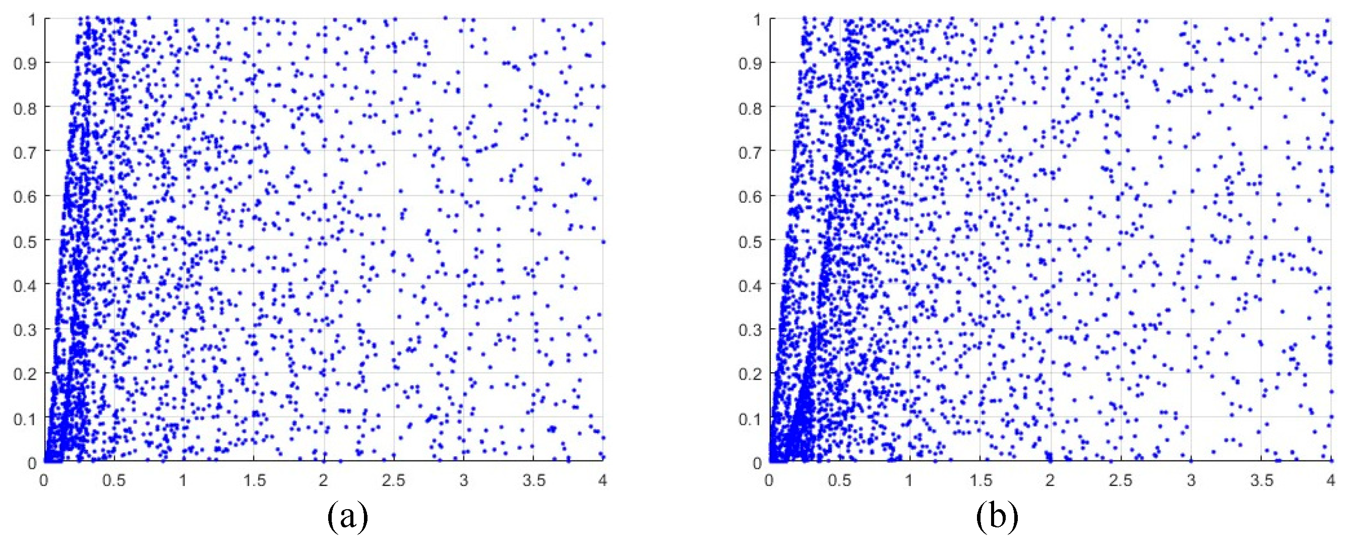
Figure 3.
Trajectory plots. (a) 2D-LM, (b) 2D-SLMM, (c) 2D-LALM, (d) 2D-LSMCL, (e) 2D-CLSS, and (f) 2D-CHSLM.
Figure 3.
Trajectory plots. (a) 2D-LM, (b) 2D-SLMM, (c) 2D-LALM, (d) 2D-LSMCL, (e) 2D-CLSS, and (f) 2D-CHSLM.
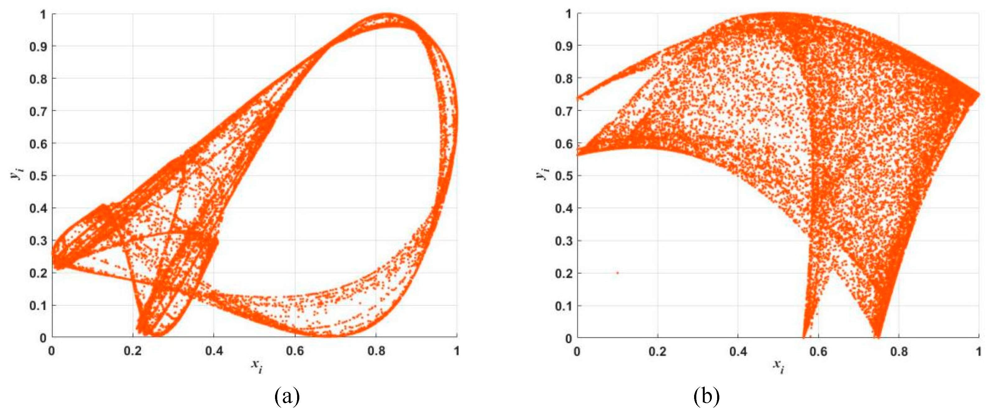
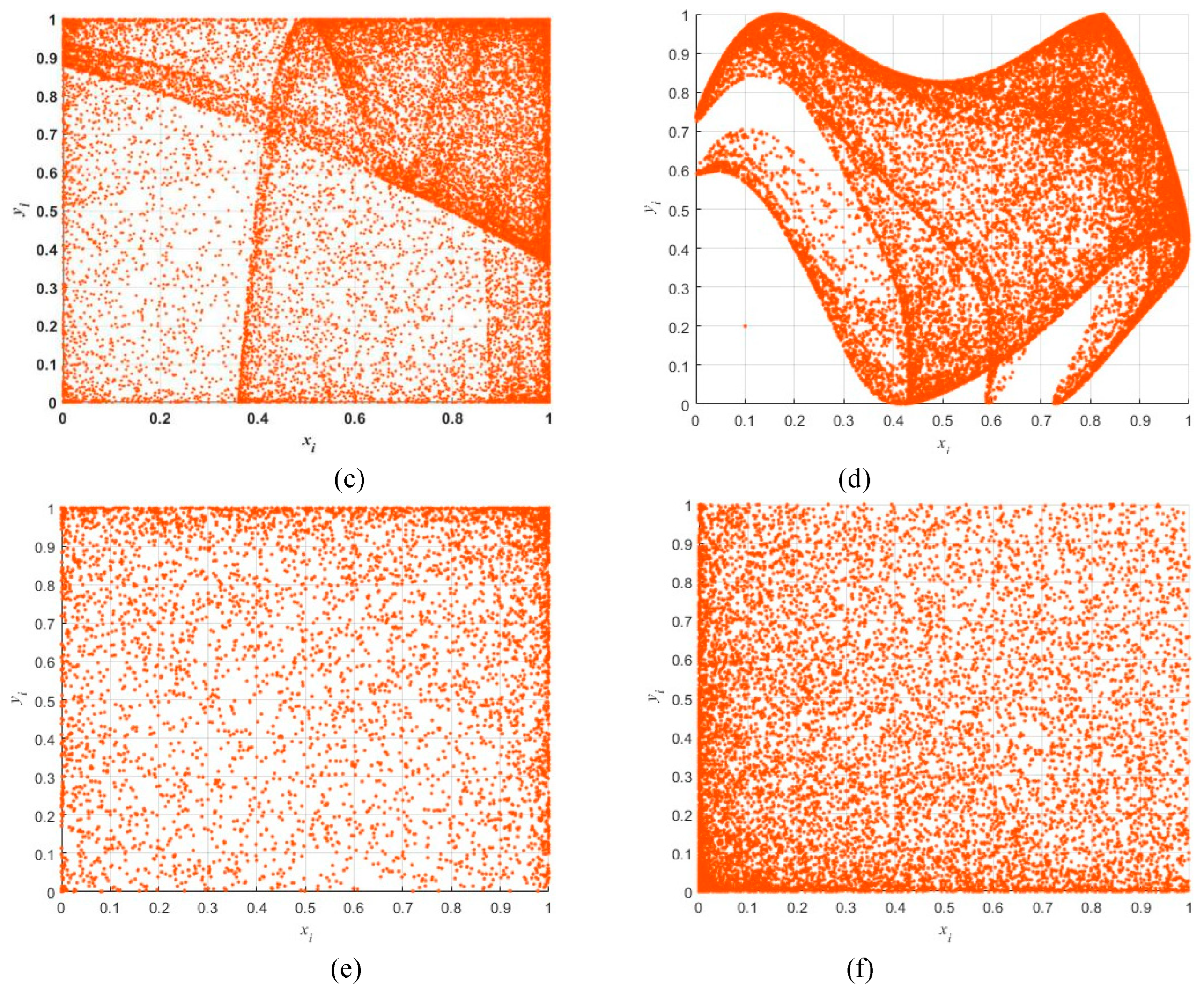
Figure 4.
Variation of LE ( and ) of (a) 2D-LM, (b) 2D-SLMM, (c) 2D-LALM, (d) 2D-LSMCL, (e) 2D-CLSS, and (f) 2D-CHSLM.
Figure 4.
Variation of LE ( and ) of (a) 2D-LM, (b) 2D-SLMM, (c) 2D-LALM, (d) 2D-LSMCL, (e) 2D-CLSS, and (f) 2D-CHSLM.
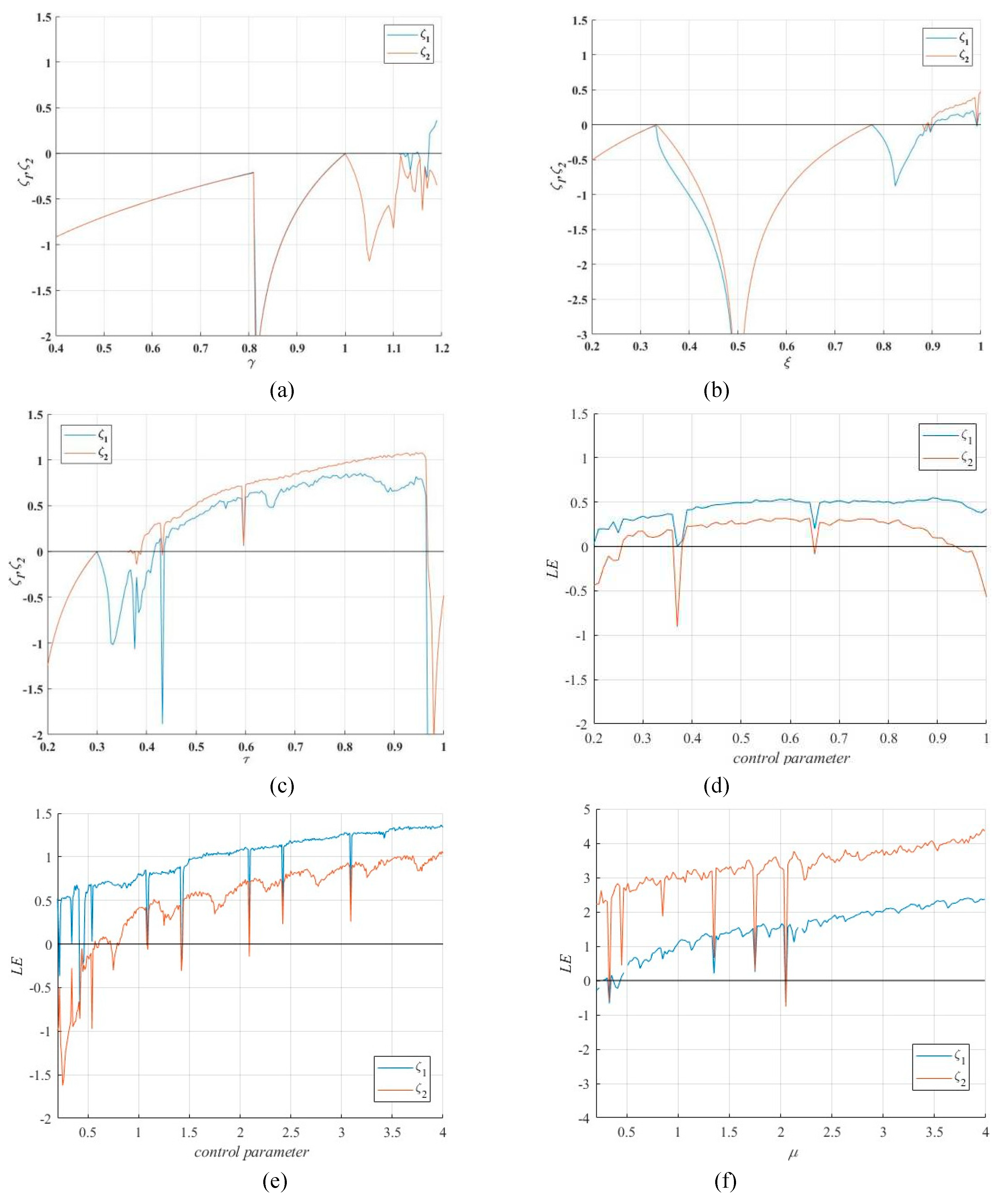
Figure 5.
Variation of SE values of (a) 2D-LM, (b) 2D-SLMM, (c) 2D-LALM, (d) 2D-LSMCL, (e) 2D-CLSS, and (f) 2D-CHSLM.
Figure 5.
Variation of SE values of (a) 2D-LM, (b) 2D-SLMM, (c) 2D-LALM, (d) 2D-LSMCL, (e) 2D-CLSS, and (f) 2D-CHSLM.
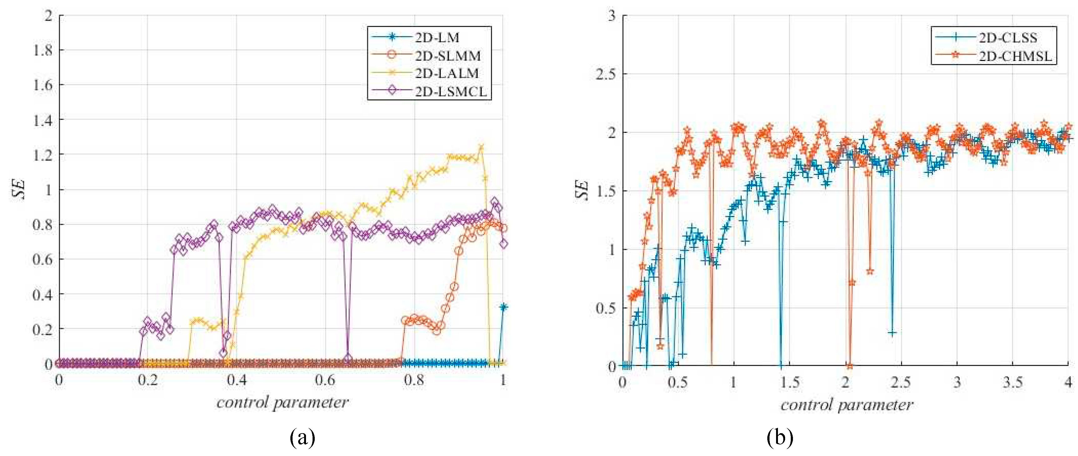
Figure 6.
Variation of C0 values of (a) 2D-LM, (b) 2D-SLMM, (c) 2D-LALM, (d) 2D-LSMCL, (e) 2D-CLSS, and (f) 2D-CHSLM.
Figure 6.
Variation of C0 values of (a) 2D-LM, (b) 2D-SLMM, (c) 2D-LALM, (d) 2D-LSMCL, (e) 2D-CLSS, and (f) 2D-CHSLM.
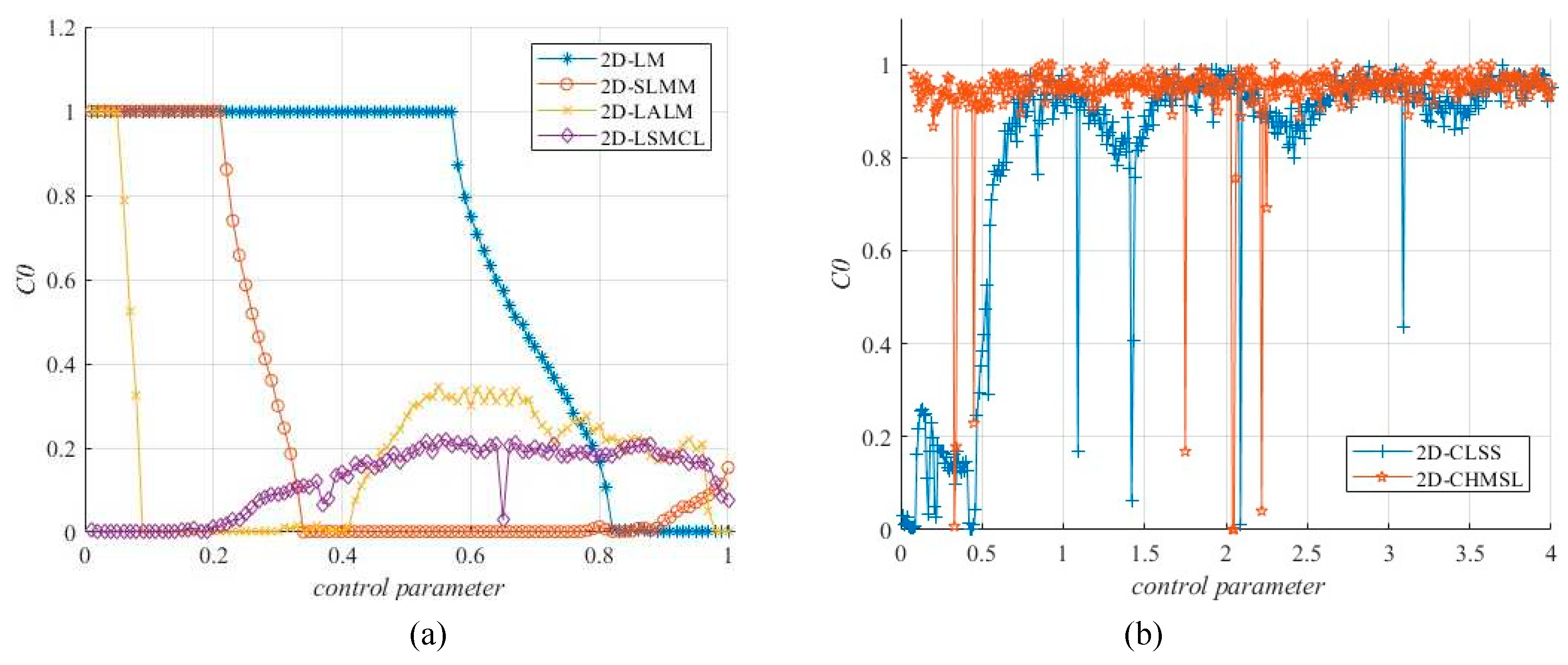
Figure 7.
Variation of PE values of (a) 2D-LM, (b) 2D-SLMM, (c) 2D-LALM, (d) 2D-LSMCL, (e) 2D-CLSS, and (f) 2D-CHSLM.
Figure 7.
Variation of PE values of (a) 2D-LM, (b) 2D-SLMM, (c) 2D-LALM, (d) 2D-LSMCL, (e) 2D-CLSS, and (f) 2D-CHSLM.
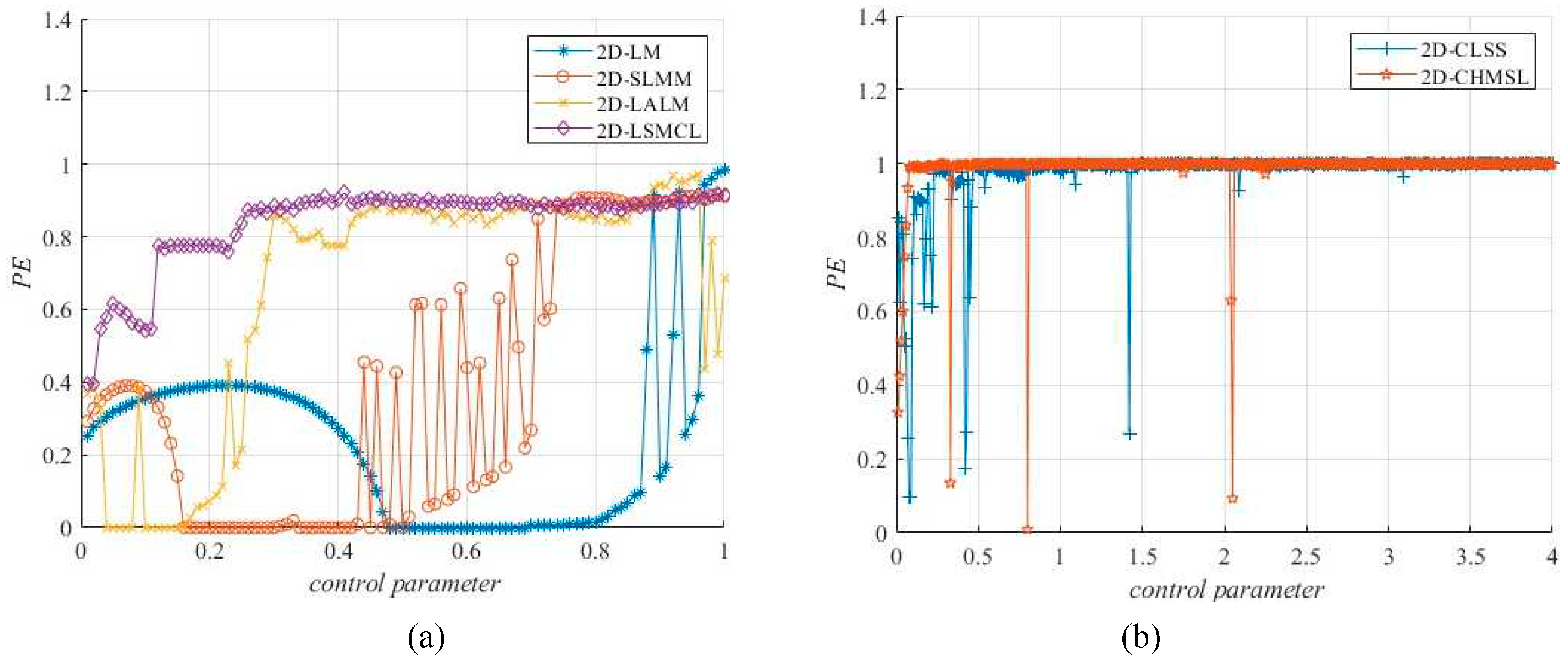
Figure 8.
The asymptotic growth rate : 2D CLSS at (a) and (b) , and 2D-CHSLM at (c) and (d) .
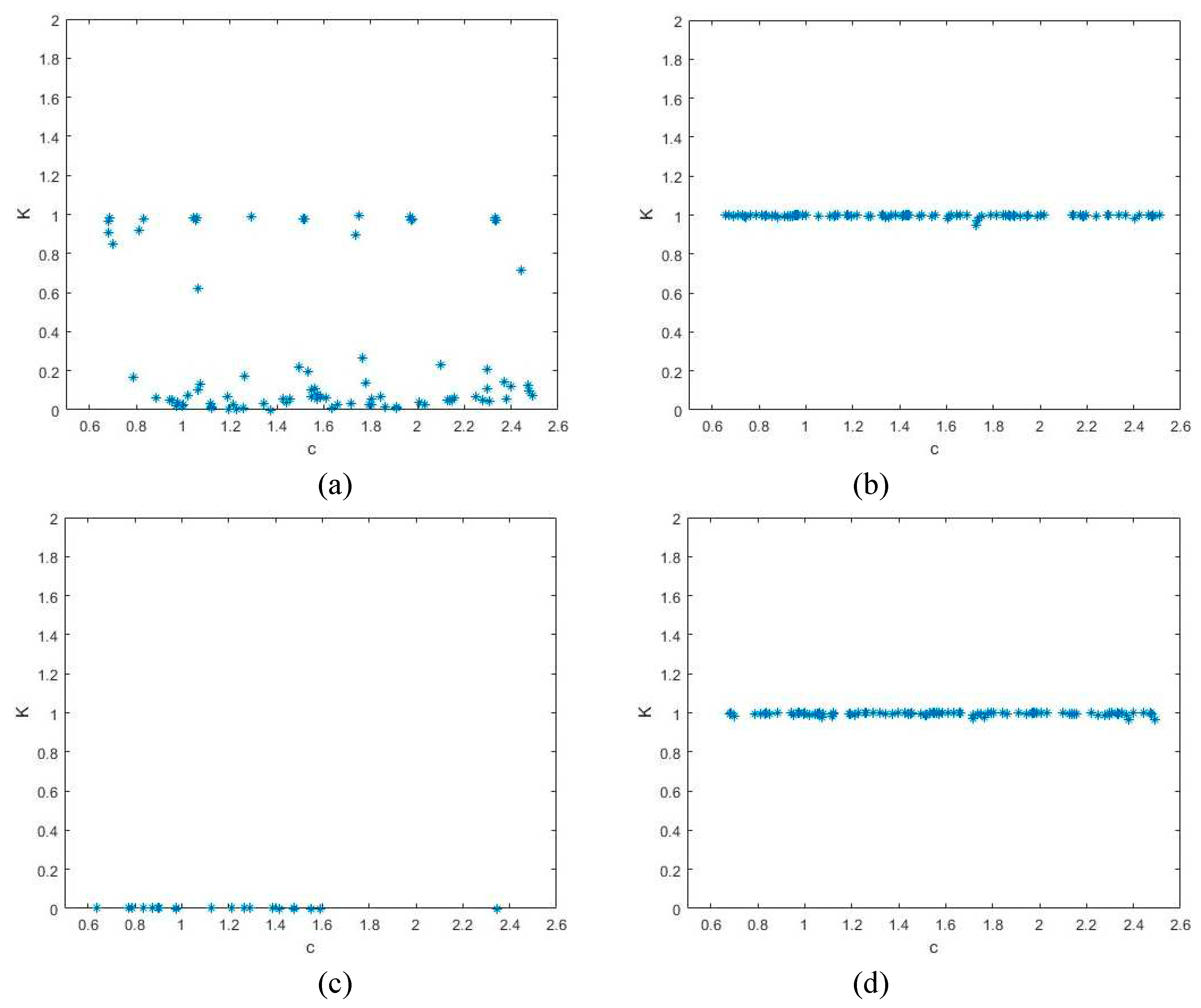
Figure 9.
Zig-zag transform: a zig-zag path with starting pixel (a) (1,1) and (b) (4,4), the scanned result of (c) Figure 9(a) and (d) Figure 9(b).
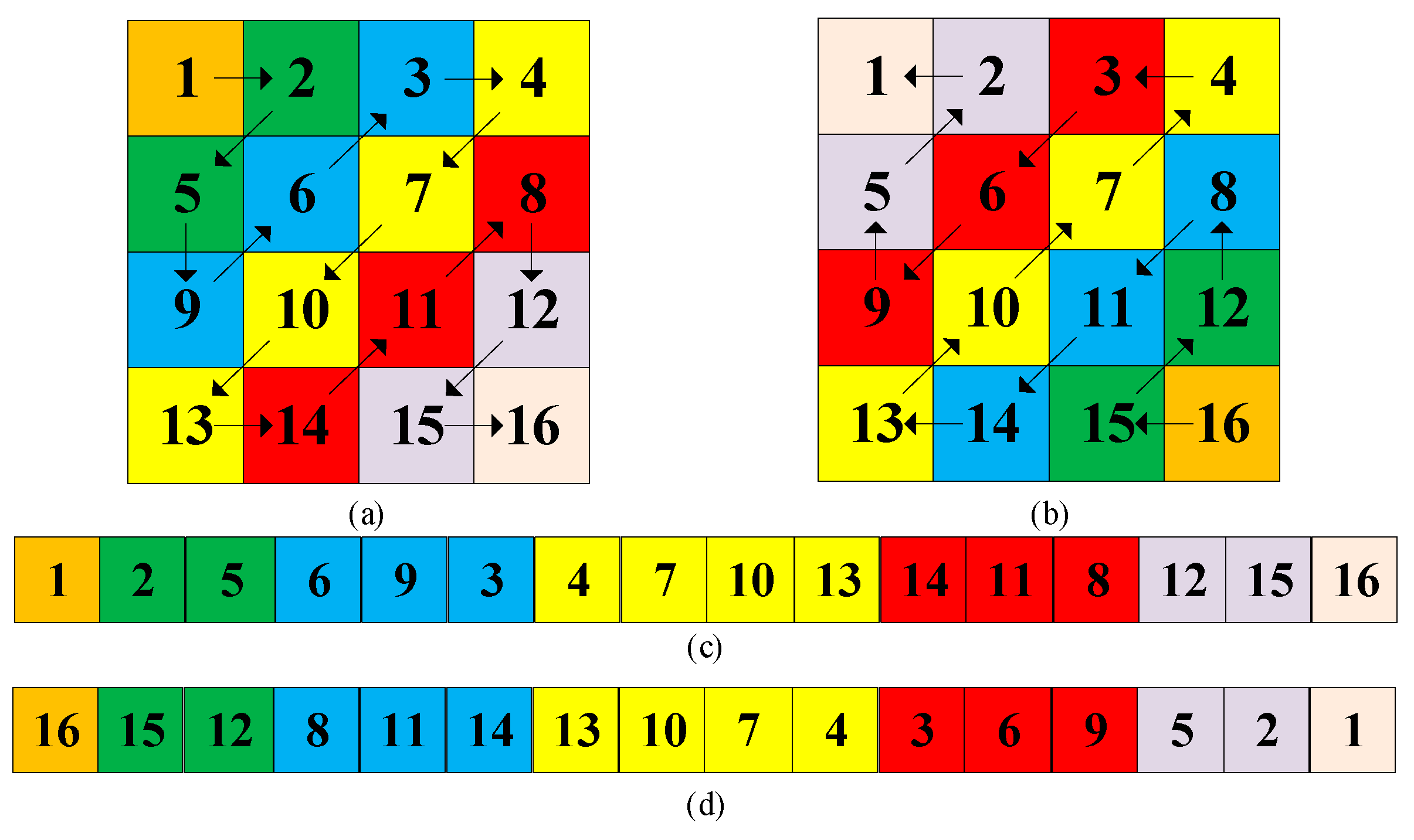
Figure 11.
The structure of .
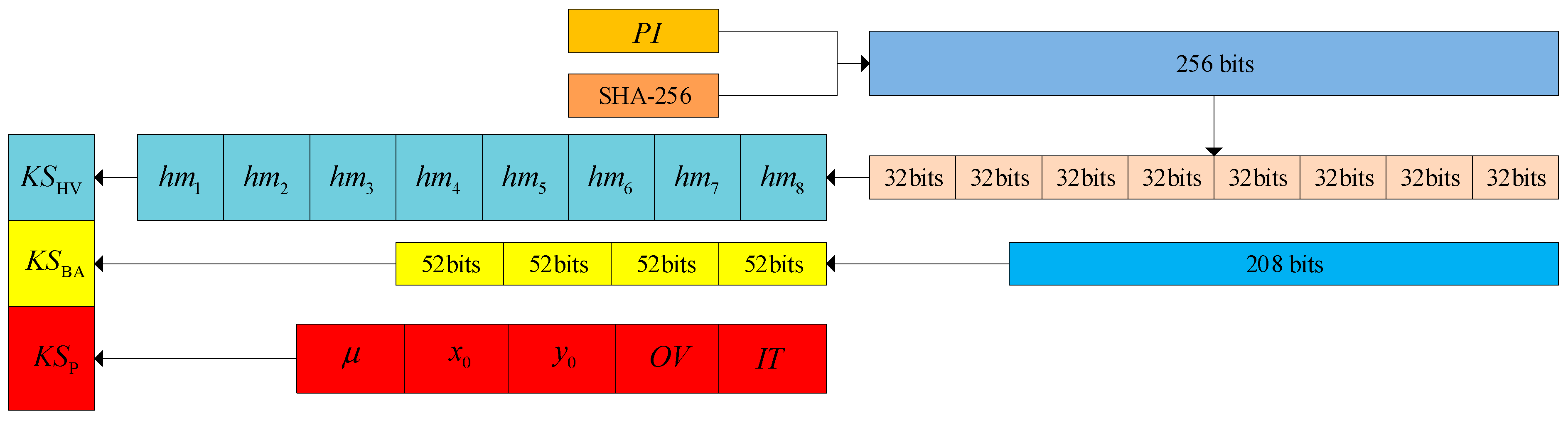
Figure 12.
The flowchart of 2D-CHSLM-IES.
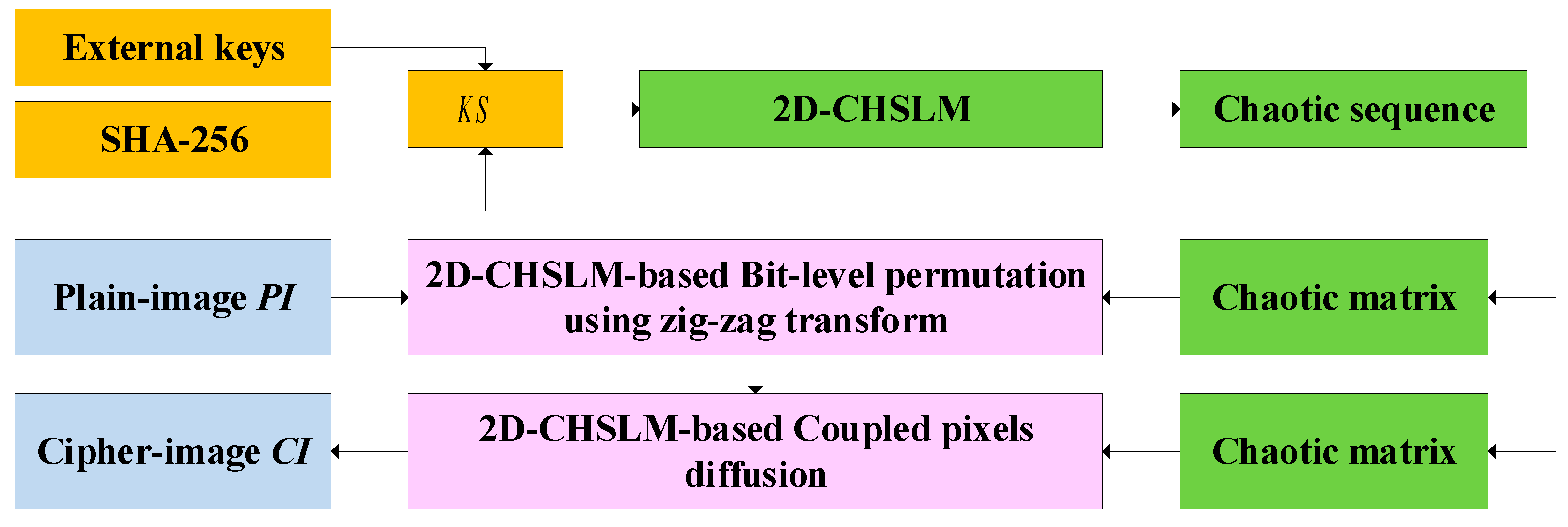
Figure 13.
The plain, cipher and decrypted images of 2D-CHSLM-IES: the plain-image (a) 5.1.11, (b) 5.2.08, (c) boat.512, and (d) 5.3.01, the cipher-image of (e) Figure 13(a), (f) Figure 13(b), (g) Figure 13(c), and (h) Figure 13(d), and the decrypted image of (i) Figure 13(e), (j) Figure 13(f), (k) Figure 13(g), and (l) Figure 13(h).
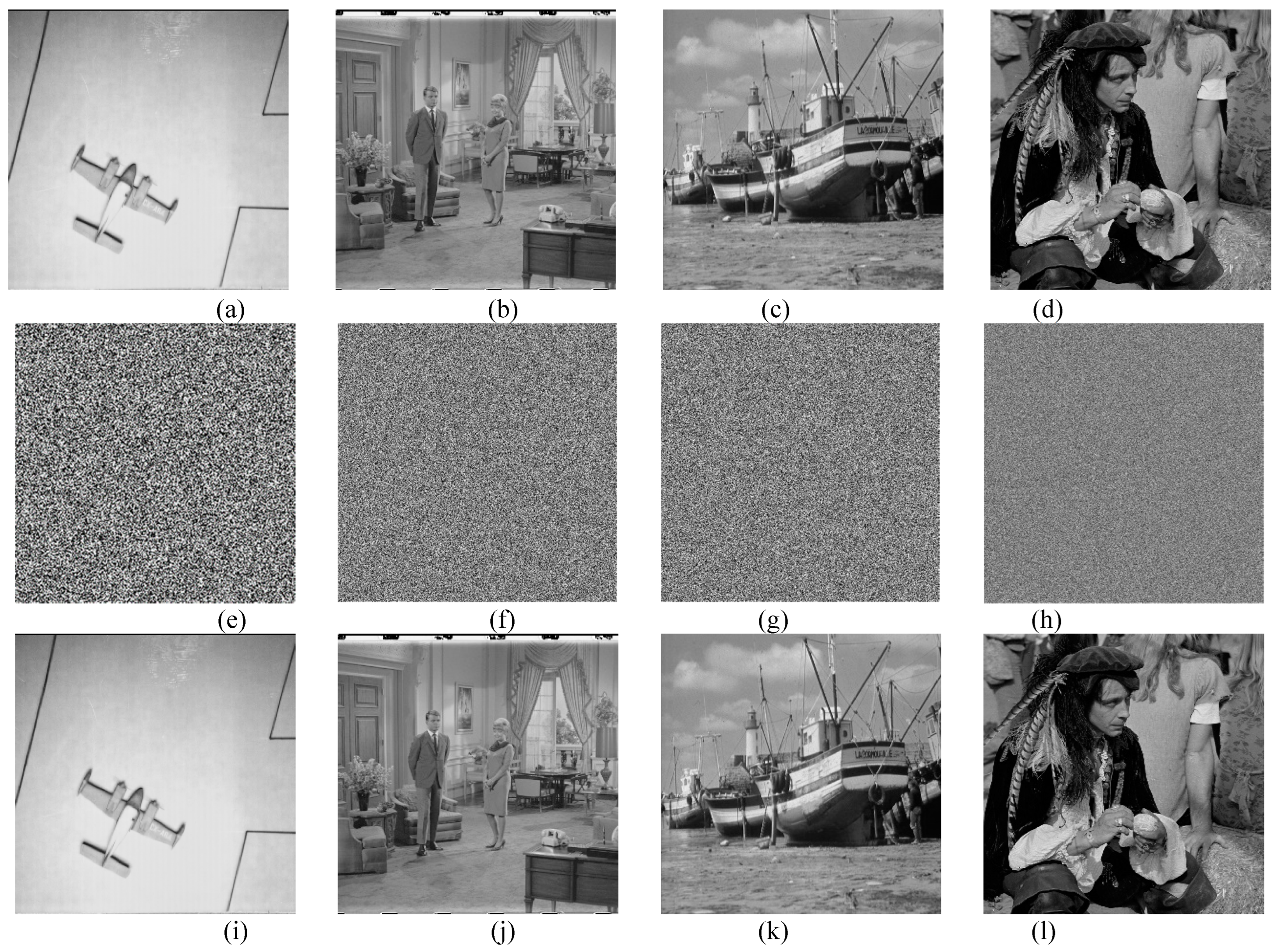
Figure 14.
Key sensitivity result: (a) the plain image “5.1.09”, the cipher-image of Figure 14(a) using (b) and (c) , (d) the differential image of Figure 14(b) and (c), the decoded image of Figure 14(b) using (e) and (f), the decoded image of Figure 14(c) using (g) and (h) .
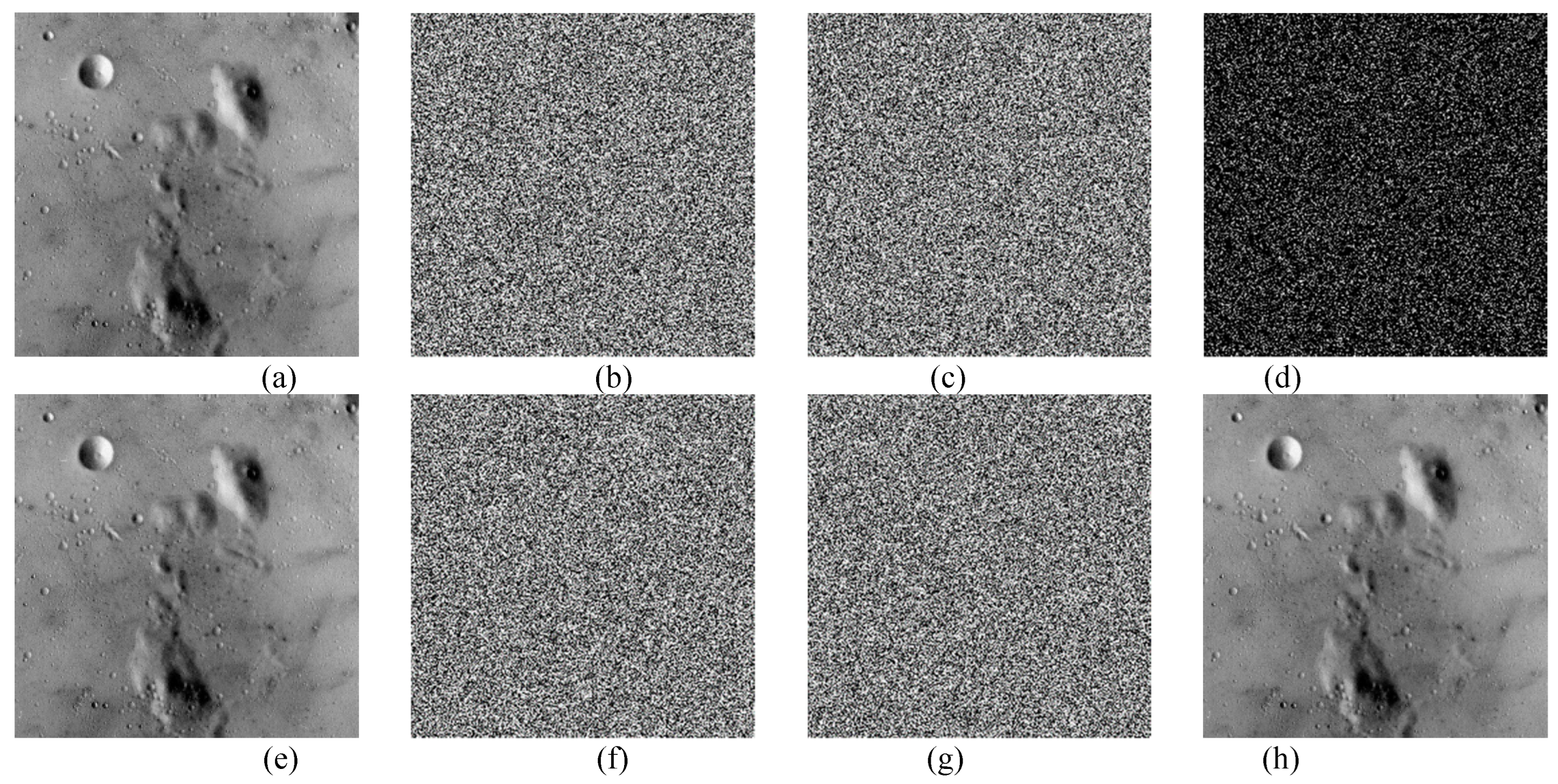
Figure 15.
Histogram: (a) the plain-image 5.1.11 and the histogram of (b) Figure 14(a), (c) the cipher-image of 5.1.11 and the histogram of (d) Figure 15(c).
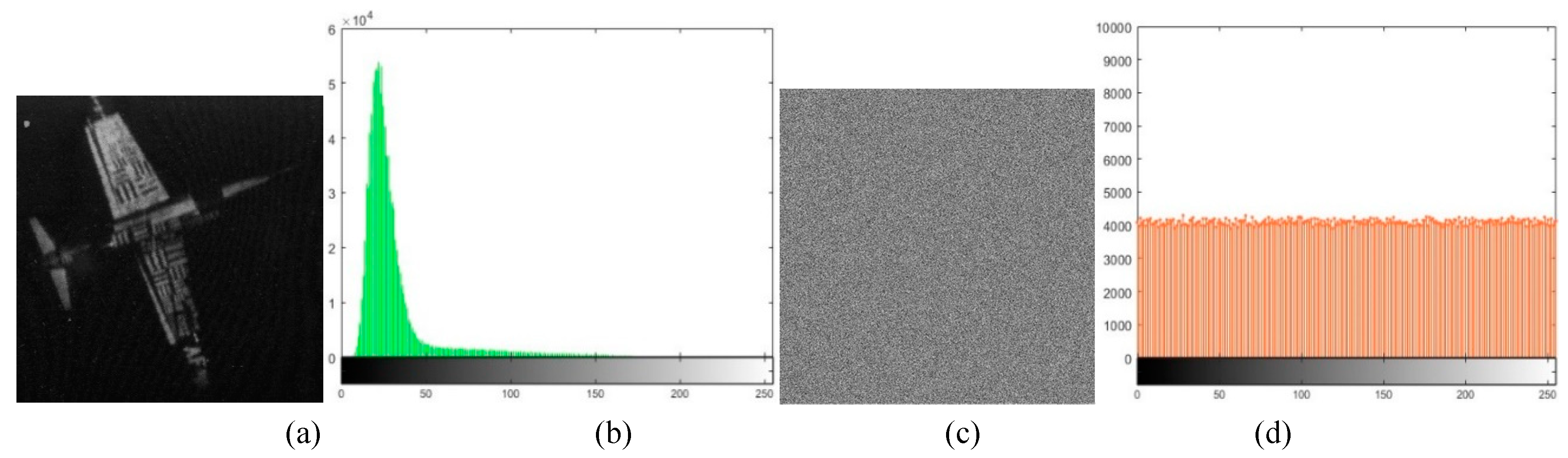
Figure 16.
Correlation analysis: (a) the plain-image “5.1.12” and (b) the adjacent pixel correlation on three directions; the cipher-image of Figure 16(a) and (d) the adjacent pixel correlation on three directions.
Figure 16.
Correlation analysis: (a) the plain-image “5.1.12” and (b) the adjacent pixel correlation on three directions; the cipher-image of Figure 16(a) and (d) the adjacent pixel correlation on three directions.
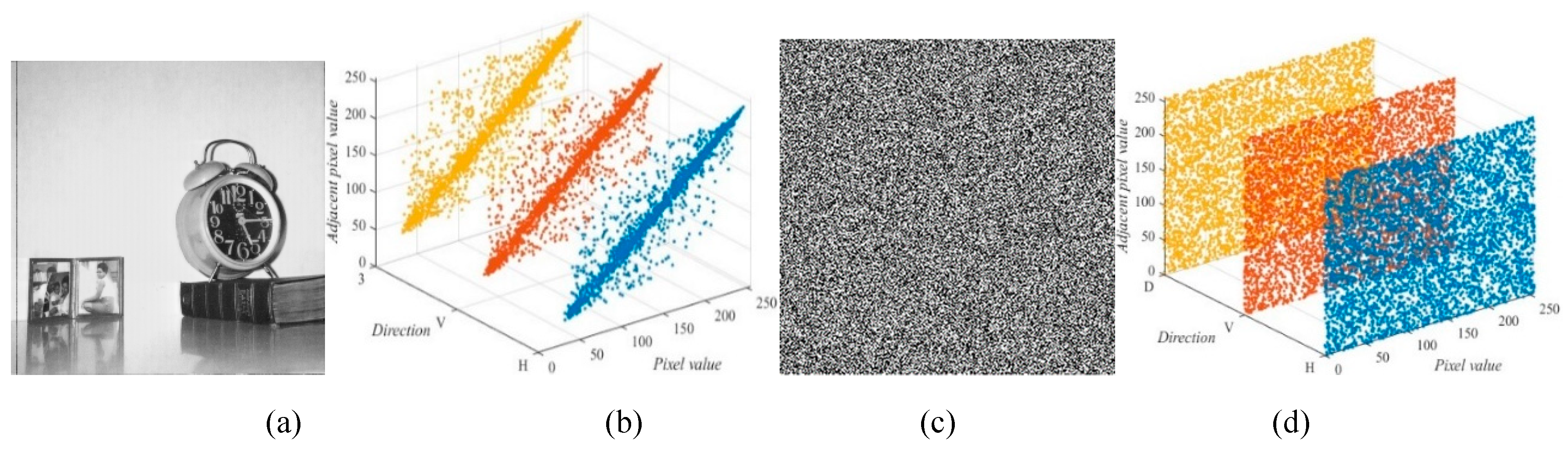
Figure 17.
Noise attacks: the cipher-image “gray21.512” with the salt-and-pepper noise intensity of (a) 0.01 and (b) 0.05 , and the speckle noise intensity of (c) 0.0001 and (d) 0.0005 , Figure 17(e-h) are the cipher-image of Figure 17(a-d).
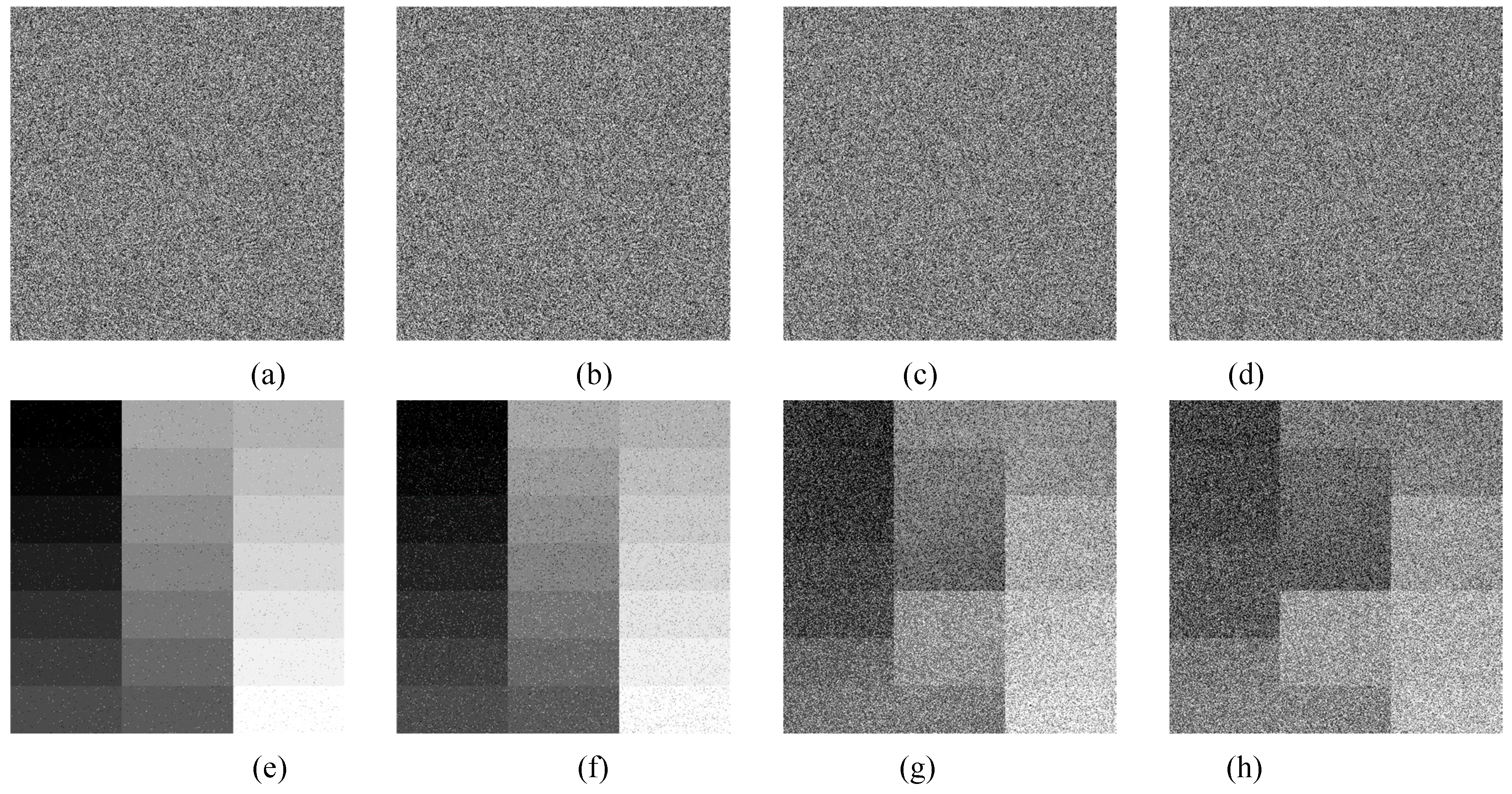
Figure 18.
Data loss attacks: the cipher-image “5.3.1” lose data with (a), (b) and (c), respectively; and the decoded image of (d) Figure 18(a), (e) Figure 18(b), and (h) Figure 18(c).
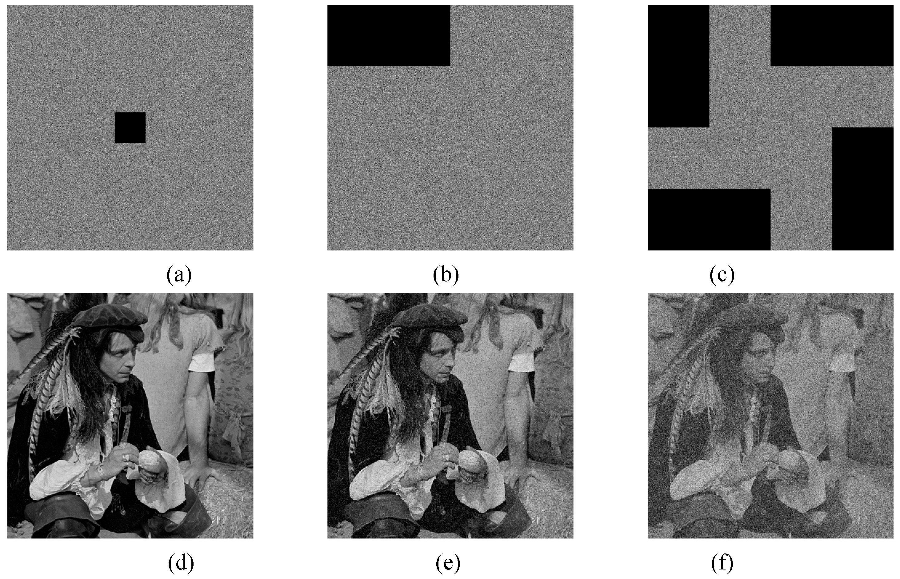

Table 1.
test results.
| Test image | Size | P-values | Decision (H=0 or 1) | ||
| 5.1.09 | 253.2188 | 0.1940 | 0 | Accepted | |
| 5.1.10 | 230.9609 | 0.7099 | 0 | Accepted | |
| 5.1.11 | 218.9922 | 0.6540 | 0 | Accepted | |
| 5.1.12 | 240.5078 | 0.3791 | 0 | Accepted | |
| 5.1.14 | 240.1172 | 0.1339 | 0 | Accepted | |
| 5.2.08 | 269.8145 | 0.7031 | 0 | Accepted | |
| 5.2.09 | 236.5098 | 0.2511 | 0 | Accepted | |
| 5.2.10 | 276.7363 | 0.4475 | 0 | Accepted | |
| 7.1.01 | 268.9434 | 0.5625 | 0 | Accepted | |
| 7.1.02 | 315.0625 | 0.2259 | 0 | Accepted | |
| 7.1.03 | 242.1719 | 0.0453 | 0 | Accepted | |
| 7.1.04 | 235.498 | 0.9711 | 0 | Accepted | |
| 7.1.05 | 292.6602 | 0.5090 | 0 | Accepted | |
| 7.1.06 | 237.9414 | 0.2222 | 0 | Accepted | |
| 7.1.07 | 311.0371 | 0.2414 | 0 | Accepted | |
| 7.1.08 | 225.7656 | 0.2992 | 0 | Accepted | |
| 7.1.09 | 302.6230 | 0.3242 | 0 | Accepted | |
| 7.1.10 | 225.2598 | 0.2378 | 0 | Accepted | |
| boat.512 | 267.3926 | 0.1914 | 0 | Accepted | |
| gray21.512 | 266.9336 | 0.2579 | 0 | Accepted | |
| 5.3.01 | 337.5430 | 0.0850 | 0 | Accepted | |
| 5.3.02 | 316.2832 | 0.3871 | 0 | Accepted | |
| 7.2.01 | 413.6880 | 0.1055 | 0 | Accepted |
Table 2.
The variance values for different key sets.
| Test image | |||||
| 5.1.09 | 5441.8550 | 5485.7893 | 5485.2374 | 5448.9941 | 5432.9961 |
| 5.1.10 | 5447.6739 | 5493.1078 | 5457.2804 | 5456.3162 | 5447.6196 |
| 5.1.11 | 5496.4997 | 5449.3551 | 5460.8342 | 5472.1545 | 5493.2718 |
| 5.1.12 | 5458.7555 | 5453.2077 | 5466.7498 | 5480.9086 | 5460.4149 |
| 5.1.14 | 5459.1291 | 5442.7278 | 5477.9664 | 5457.8505 | 5459.0039 |
| 5.2.08 | 5459.5898 | 5459.0095 | 5457.9681 | 5454.6884 | 5459.5509 |
| 5.2.09 | 5452.3726 | 5449.8282 | 5466.6573 | 5458.529 | 5452.3228 |
| 5.2.10 | 5472.2117 | 5468.2702 | 5463.4145 | 5432.299 | 5472.0094 |
| 7.1.01 | 5474.1376 | 5460.8777 | 5475.4914 | 5462.9336 | 5474.935 |
| 7.1.02 | 5467.3954 | 5474.5296 | 5476.7792 | 5470.1655 | 5467.7073 |
| 7.1.03 | 5453.6022 | 5451.4377 | 5454.1955 | 5449.8652 | 5452.765 |
| 7.1.04 | 5474.5494 | 5459.1821 | 5446.8977 | 5456.0021 | 5472.9866 |
| 7.1.05 | 5462.1370 | 5446.5362 | 5460.1792 | 5460.415 | 5461.4496 |
| 7.1.06 | 5467.9458 | 5457.9691 | 5455.3284 | 5451.521 | 5467.192 |
| 7.1.07 | 5474.8764 | 5455.9308 | 5465.7357 | 5466.7098 | 5474.9154 |
| 7.1.08 | 5446.7922 | 5467.8586 | 5455.8798 | 5462.2921 | 5447.1123 |
| 7.1.09 | 5455.3019 | 5456.5913 | 5470.0106 | 5465.4739 | 5454.0027 |
| 7.1.10 | 5467.5594 | 5479.9682 | 5477.0743 | 5451.5287 | 5468.2064 |
| boat.512 | 5453.1570 | 5456.1997 | 5462.1926 | 5469.9872 | 5451.3742 |
| gray21.512 | 5448.9852 | 5448.5082 | 5455.3162 | 5459.1326 | 5448.9232 |
| 5.3.01 | 5463.5445 | 5461.2454 | 5461.4147 | 5458.3164 | 5463.4359 |
| 5.3.02 | 5469.0697 | 5462.018 | 5467.0965 | 5456.1629 | 5469.5559 |
| 7.2.01 | 5459.3065 | 5459.6969 | 5458.9651 | 5464.6389 | 5459.9138 |
Table 3.
Percentage of variances difference.
| Test image | ||||
| 5.1.09 | 0.8 | 0.79 | 0.13 | 0.16 |
| 5.1.10 | 0.83 | 0.18 | 0.16 | 0,001 |
| 5.1.11 | 0.87 | 0.65 | 0.44 | 0.06 |
| 5.1.12 | 0.1 | 0.15 | 0.4 | 0.03 |
| 5.1.14 | 0.3 | 0.34 | 0.02 | 0.002 |
| 5.2.08 | 0.01 | 0.03 | 0.09 | 0.001 |
| 5.2.09 | 0.05 | 0.26 | 0.11 | 0.001 |
| 5.2.10 | 0.07 | 0.16 | 0.73 | 0.004 |
| 7.1.01 | 0.24 | 0.02 | 0.21 | 0.01 |
| 7.1.02 | 0.13 | 0.17 | 0.05 | 0.01 |
| 7.1.03 | 0.04 | 0.01 | 0.07 | 0.02 |
| 7.1.04 | 0.28 | 0.51 | 0.34 | 0.03 |
| 7.1.05 | 0.29 | 0.04 | 0.03 | 0.01 |
| 7.1.06 | 0.18 | 0.23 | 0.3 | 0.01 |
| 7.1.07 | 0.35 | 0.17 | 0.15 | 0.001 |
| 7.1.08 | 0.39 | 0.17 | 0.28 | 0.01 |
| 7.1.09 | 0.02 | 0.27 | 0.19 | 0.02 |
| 7.1.10 | 0.23 | 0.17 | 0.29 | 0.01 |
| boat.512 | 0.06 | 0.17 | 0.31 | 0.03 |
| gray21.512 | 0.01 | 0.12 | 0.19 | 0.001 |
| 5.3.01 | 0.04 | 0.04 | 0.1 | 0.002 |
| 5.3.02 | 0.13 | 0.04 | 0.24 | 0.01 |
| 7.2.01 | 0.01 | 0.01 | 0.1 | 0.01 |
| Mean | 0.24 | 0.20 | 0.21 | 0.02 |
Table 4.
Correlations of two adjacent pixels on three directions and their comparison results.
| Test image | 2D-CHSLM-IES | Ref. [41] | |||||||
| Plain-image | Cipher-image | Cipher-image | |||||||
| H | V | D | H | V | D | H | V | D | |
| 5.1.09 | 0.9094 | 0.9053 | 0.8989 | 0.003 | -0.0029 | -0.0017 | 0.0162 | -0.0139 | 0.0025 |
| 5.1.10 | 0.8242 | 0.8047 | 0.7928 | 0.0012 | -0.0034 | 0.0016 | -0.0258 | 0.0041 | 0.0009 |
| 5.1.11 | 0.8898 | 0.8512 | 0.9212 | 0.001 | 0.0029 | 0.0019 | -0.0016 | -0.0012 | 0.0141 |
| 5.1.12 | 0.9485 | 0.9498 | 0.9308 | 0.0031 | -0.0033 | -0.0018 | -0.0114 | -0.0097 | 0.0034 |
| 5.1.13 | 0.7512 | 0.7549 | 0.7874 | 0.0042 | 0.0048 | 0.0015 | 0.0070 | 0.0100 | -0.0097 |
| 5.1.14 | 0.8583 | 0.8597 | 0.856 | -0.0012 | 0.0011 | -0.004 | -0.0176 | -0.0054 | -0.0196 |
| 5.2.08 | 0.8387 | 0.8374 | 0.8813 | -0.0012 | -0.0032 | -0.002 | -0.0028 | 0.0046 | 0.0124 |
| 5.2.09 | 0.7839 | 0.8213 | 0.817 | -0.001 | -0.0016 | 0.0031 | -0.0172 | -0.0091 | -0.0178 |
| 5.2.10 | 0.8824 | 0.9038 | 0.901 | -0.0028 | -0.0011 | 0.0036 | -0.0190 | 0.0005 | -0.0050 |
| 7.1.01 | 0.8975 | 0.9038 | 0.9128 | -0.0024 | -0.0024 | 0.0023 | 0.0195 | -0.0070 | -0.0165 |
| 7.1.02 | 0.9038 | 0.897 | 0.8766 | -0.0025 | 0.0026 | -0.0047 | 0.0291 | -0.0176 | -0.0080 |
| 7.1.03 | 0.8924 | 0.8931 | 0.8983 | -0.0016 | 0.003 | -0.0019 | -0.0293 | -0.0091 | 0.0086 |
| 7.1.04 | 0.9607 | 0.9529 | 0.9543 | 0.0015 | -0.0022 | -0.0018 | -0.0005 | 0.0026 | 0.0030 |
| 7.1.05 | 0.8827 | 0.8932 | 0.8949 | -0.0013 | 0.0032 | -0.0007 | -0.0126 | 0.0044 | 0.0004 |
| 7.1.06 | 0.8787 | 0.8772 | 0.8743 | 0.0037 | 0.0017 | -0.003 | 0.0161 | 0.0110 | 0.0032 |
| 7.1.07 | 0.8436 | 0.8454 | 0.8444 | -0.0001 | -0.0029 | -0.0028 | 0.0017 | -0.0194 | -0.0076 |
| 7.1.08 | 0.9208 | 0.9114 | 0.9276 | 0.0023 | -0.0041 | -0.0035 | 0.0006 | -0.0142 | 0.00002 |
| 7.1.09 | 0.9187 | 0.9135 | 0.9073 | 0.0039 | -0.0029 | -0.0036 | -0.0047 | 0.0149 | 0.0089 |
| 7.1.10 | 0.9192 | 0.9423 | 0.9437 | 0.0047 | 0.0048 | 0.0035 | 0.0051 | -0.0109 | 0.0144 |
| boat.512 | 0.9257 | 0.9405 | 0.9276 | 0.0035 | 0.0008 | -0.0048 | -0.0045 | -0.0011 | -0.0113 |
| gray21.512 | 0.999 | 0.994 | 0.9974 | 0.0011 | 0.0012 | 0.0042 | -0.0086 | -0.0145 | 0.0068 |
| ruler.512 | 0.0425 | -0.0708 | -0.0811 | -0.0014 | 0.0025 | -0.0025 | -0.0035 | -0.0085 | 0.0165 |
| 5.3.01 | 0.9665 | 0.9625 | 0.9694 | -0.0022 | 0.0035 | -0.0037 | -0.0057 | -0.0069 | 0.0040 |
| 5.3.02 | 0.8712 | 0.8444 | 0.8557 | 0.0027 | -0.0004 | -0.0035 | -0.0137 | 0.0007 | 0.0091 |
| 7.2.01 | 0.9398 | 0.9562 | 0.9486 | 0.0024 | 0.0012 | 0.0026 | -0.0032 | 0.0032 | 0.0047 |
Table 5.
Information entropy results of 2D-CHSLM-IES and their comparison results.
| Test image | Plain-image | Cipher-image | |||
| Ref. [41] | Ref. [42] | Ref. [43] | 2D-CHSLM-IES | ||
| 5.1.09 | 6.7057 | 7.996950 | 7.9973 | 7.9972 | 7.9972 |
| 5.1.10 | 1.5483 | 7.997474 | 7.9973 | 7.9977 | 7.9975 |
| 5.1.11 | 7.3424 | 7.997126 | 7.9968 | 7.9971 | 7.9976 |
| 5.1.12 | 7.2010 | 7.997025 | 7.9975 | 7.9972 | 7.9973 |
| 5.1.13 | 6.9940 | 7.996947 | 7.9975 | 7.9970 | 7.9972 |
| 5.1.14 | 5.7056 | 7.997028 | 7.9973 | 7.9970 | 7.9973 |
| 5.2.08 | 6.0274 | 7.999341 | 7.9993 | 7.9993 | 7.9993 |
| 5.2.09 | 4.0045 | 7.999300 | 7.9992 | 7.9991 | 7.9993 |
| 5.2.10 | 5.4957 | 7.999381 | 7.9993 | 7.9991 | 7.9992 |
| 7.1.01 | 6.1074 | 7.999235 | 7.9993 | 7.9993 | 7.9993 |
| 7.1.02 | 6.5632 | 7.999330 | 7.9993 | 7.9994 | 7.9991 |
| 7.1.03 | 6.6953 | 7.999262 | 7.9993 | 7.9993 | 7.9993 |
| 7.1.04 | 5.9916 | 7.999299 | 7.9993 | 7.9994 | 7.9994 |
| 7.1.05 | 5.0534 | 7.999333 | 7.9994 | 7.9992 | 7.9992 |
| 7.1.06 | 6.1898 | 7.999267 | 7.9992 | 7.9993 | 7.9993 |
| 7.1.07 | 5.9088 | 7.999211 | 7.9994 | 7.9993 | 7.9991 |
| 7.1.08 | 7.1914 | 7.999171 | - | 7.9993 | 7.9994 |
| 7.1.09 | 4.3923 | 7.999268 | - | 7.9993 | 7.9992 |
| 7.1.10 | 0.5000 | 7.999337 | - | 7.9992 | 7.9994 |
| boat.512 | 7.5237 | 7.999179 | 7.9993 | 7.9993 | 7.9993 |
| gray21.512 | 6.8303 | 7.999454 | 7.9993 | 7.9994 | 7.9993 |
| ruler.512 | 5.6415 | 7.999270 | 7.9993 | 7.9992 | 7.9991 |
| 5.3.01 | 6.7057 | 7.999829 | 7.9998 | 7.9998 | 7.9998 |
| 5.3.02 | 1.5483 | 7.999851 | 7.9998 | 7.9998 | 7.9998 |
| 7.2.01 | 7.3424 | 7.999821 | 7.9998 | 7.9998 | 7.9997 |
| Mean of | 6.0116 | 7.997091 | 7.9973 | 7.9972 | 7.9974 |
| Mean of | 5.6263 | 7.999290 | 7.9993 | 7.9993 | 7.9993 |
| Mean of | 6.6652 | 7.999834 | 7.9998 | 7.9998 | 7.9998 |
Table 6.
Ranges of and ().
| , | Critical values () | ||
| 99.5693 | 99.5893 | 99.5994 | |
| 33.2824 | 33.3730 | 33.4182 | |
| 33.6447 | 33.5541 | 33.5088 | |
Table 7.
and (b) , and the speckle noise intensity of (c) and (d) , Figure 17(e-h) are the cipher-image of Figure 17(a-d).
| Test image | ||||||||
| Ref. [41] | Ref. [42] | Ref. [43] | 2D-CHSLM-IES | Ref. [41] | Ref. [42] | Ref. [43] | 2D-CHSLM-IES | |
| 5.1.09 | 99.6002 | 99.6323 | 99.6094 | 99.6109 | 33.4831 | 33.4561 | 33.4817 | 33.4330 |
| 5.1.10 | 99.6170 | 99.6124 | 99.6185 | 99.6140 | 33.5384 | 33.5674 | 33.4672 | 33.4606 |
| 5.1.11 | 99.6292 | 99.6078 | 99.6048 | 99.6185 | 33.5100 | 33.4934 | 33.4216 | 33.4543 |
| 5.1.12 | 99.6109 | 99.6185 | 99.6094 | 99.6231 | 33.3905 | 33.4669 | 33.4362 | 33.5017 |
| 5.1.13 | 99.6307 | 99.5956 | 99.6109 | 99.6124 | 33.4601 | 33.4151 | 33.4393 | 33.4913 |
| 5.1.14 | 99.5911 | 99.6292 | 99.6002 | 99.6353 | 33.4052 | 33.4585 | 33.4646 | 33.4260 |
| 5.2.08 | 99.5972 | 99.6193 | 99.6109 | 99.6265 | 33.4380 | 33.4772 | 33.4865 | 33.4330 |
| 5.2.09 | 99.6265 | 99.6178 | 99.6090 | 99.6098 | 33.5115 | 33.4369 | 33.4788 | 33.4977 |
| 5.2.10 | 99.6216 | 99.6323 | 99.6086 | 99.6059 | 33.5257 | 33.4081 | 33.5094 | 33.4794 |
| 7.1.01 | 99.6098 | 99.6204 | 99.6071 | 99.6040 | 33.4190 | 33.4324 | 33.4632 | 33.4694 |
| 7.1.02 | 99.6189 | 99.6101 | 99.6094 | 99.6212 | 33.5257 | 33.4435 | 33.4572 | 33.4410 |
| 7.1.03 | 99.6273 | 99.5975 | 99.6098 | 99.6151 | 33.5024 | 33.4653 | 33.4241 | 33.4801 |
| 7.1.04 | 99.5979 | 99.6113 | 99.6117 | 99.6014 | 33.4243 | 33.4360 | 33.4671 | 33.4845 |
| 7.1.05 | 99.6120 | 99.6159 | 99.6105 | 99.6109 | 33.4230 | 33.4468 | 33.4469 | 33.4939 |
| 7.1.06 | 99.6056 | 99.6162 | 99.6117 | 99.6124 | 33.4550 | 33.4857 | 33.4557 | 33.4338 |
| 7.1.07 | 99.6029 | 99.6086 | 99.6101 | 99.6170 | 33.4514 | 33.4385 | 33.4847 | 33.4455 |
| 7.1.08 | 99.5998 | - | 99.6162 | 99.6105 | 33.4468 | - | 33.4796 | 33.4877 |
| 7.1.09 | 99.6220 | - | 99.6071 | 99.6334 | 33.4605 | - | 33.4256 | 33.4918 |
| 7.1.10 | 99.6254 | - | 99.6109 | 99.6044 | 33.4698 | - | 33.4636 | 33.5007 |
| boat.512 | 99.6120 | 99.6078 | 99.6033 | 99.6151 | 33.4356 | 33.4853 | 33.4305 | 33.4436 |
| gray21.512 | 99.6025 | 99.6227 | 99.6094 | 99.6216 | 33.4369 | 33.4007 | 33.4916 | 33.4577 |
| ruler.512 | 99.5983 | 99.6216 | 99.6098 | 99.6033 | 33.4237 | 33.4343 | 33.5110 | 33.4847 |
| 5.3.01 | 99.6127 | 99.6024 | 99.6094 | 99.61 | 33.4455 | 33.4902 | 33.4775 | 33.4914 |
| 5.3.02 | 99.6151 | 99.6009 | 99.6076 | 99.6081 | 33.4942 | 33.4440 | 33.4646 | 33.4433 |
| 7.2.01 | 99.6058 | 99.6059 | 99.6033 | 99.6043 | 33.4597 | 33.4598 | 33.4697 | 33.4309 |
| Pass/All | 25/25 | 22/22 | 25/25 | 25/25 | 25/25 | 22/22 | 25/25 | 25/25 |
| Mean | 99.611696 | 99.6139 | 99.6092 | 99.6140 | 33.461440 | 33.4565 | 33.4639 | 33.4663 |
Disclaimer/Publisher’s Note: The statements, opinions and data contained in all publications are solely those of the individual author(s) and contributor(s) and not of MDPI and/or the editor(s). MDPI and/or the editor(s) disclaim responsibility for any injury to people or property resulting from any ideas, methods, instructions or products referred to in the content. |
© 2024 by the authors. Licensee MDPI, Basel, Switzerland. This article is an open access article distributed under the terms and conditions of the Creative Commons Attribution (CC BY) license (http://creativecommons.org/licenses/by/4.0/).
Copyright: This open access article is published under a Creative Commons CC BY 4.0 license, which permit the free download, distribution, and reuse, provided that the author and preprint are cited in any reuse.


