

Submitted:
08 May 2023
Posted:
09 May 2023
You are already at the latest version
Abstract
When there is uncertainty in the value of parameters of the input random components of a stochastic simulation model, two-level nested simulation algorithms are used to estimate the expectation of performance variables of interest. In the outer level of the algorithm (n) observations are generated for the parameters, and in the inner level (m) observations of the simulation model are generated with the value of parameters fixed at the value generated in the outer level. In this article, we consider the case in which the observations at both levels of the algorithm are independent, showing how the variance of the observations can be decomposed into the sum of a parametric variance and a stochastic variance. Next, we derive central limit theorems that allow us to compute asymptotic confidence intervals to assess the accuracy of the simulation-based estimators for the point forecast and the variance components. Under this framework, we derive analytical expressions for the point forecast and the variance components of a Bayesian model to forecast sporadic demand; and we use these expressions to illustrate the validity of our theoretical results by performing simulation experiments using this forecast model.
Keywords:
Bayesian forecasting
; stochastic simulation
; parameter uncertainty
; two-level simulation
1. Introduction and Notation
Simulation is widely recognized as an effective technique to produce forecasts, evaluate risk (see, e.g., [1]), animate and illustrate the performance of a system over time (see, e.g., [2]). When there is uncertainty in a component of a simulation model, it is said to be a random component, and it is modeled using a probability distribution and/or a stochastic process that is generated during the simulation run, to produce a stochastic simulation. Random component typically depends on the value of certain parameters, and we will denote by a particular value for the vector of parameters of the random components of a stochastic simulation, and will denote the random vector that corresponds to the parameter values when there is uncertainty on the value of these parameters.
In general, the output of a stochastic (dynamic) simulation can be regarded as a stochastic process , where is a random vector (of arbitrary dimension d) representing the state of the simulation at time . The term transient simulation applies to a dynamic simulation that has a well-defined termination time, so that the output of a transient simulation can be viewed as a stochastic process , where T is a stopping time (may be deterministic), see, e.g., [3] for a definition of stopping time. Note that this notation includes the case of a discrete-time output , if we assume that , where denotes the integer part of s.
A performance variable W in transient simulation is a real-valued random variable (r.v.) that depends on the simulation output up to time T, i.e., , and the expectation of a performance variable W is a performance measure that we usually estimate through experimentation with the simulation model. When there is no uncertainty in the parameters of the random components, the standard methodology that is used to estimate a performance measure in transient simulation is the method of independent replications, that consists on running the simulation model to produce n replications that can be regarded as independent and identically distributed (i.i.d.) random variables (see Figure 1) .
Under the method of independent replications, a point estimator for the expectation is the average . If , it follows from the classical Law of Large Numbers (LLN), that is consistent, i.e., it satisfies , as (where ⇒ denotes weak convergence of random variables), see, e.g., [3] for a proof. Consistency guarantees that the estimator approaches the parameter as the number of replications n increases, and the accuracy of the simulation-based estimator is typically assessed by an asymptotic confidence interval (ACI) for the parameter. The expression for an ACI for a parameter of a stochastic simulation is usually obtained through a Central Limit Theorem (CLT) for the estimator (see, for example, chapter 3 of [4]). For the case of the expectation in the algorithm of Figure 1, if , the classical CLT implies that
as , where and denotes a r.v. distributed as normal with mean 0 and variance 1. Then, if , it follows from (1) and Slutsky’s Theorem (see the Appendix) that
as , where denotes the sample standard deviation, i.e., . This CLT implies that
for , where denotes the ()-quantile of a N(0,1), which is sufficient to establish a ACI for with halfwidth
A halfwidth in the form of (2) is the typical measure used in simulation software (e.g., Simio, see [2]) to assess the accuracy of for the estimation of expectation .
In contrast to the estimation of (output) performance measures, parameters of (input) random components of a simulation model are usually estimated from real-data observations (x) and, while most applications covered in the relevant literature assume that no uncertainty exists in the value of these parameters, the uncertainty can be significant when little data is available. In these cases, Bayesian statistics can be used to incorporate this uncertainty in the output analysis of simulation experiments via the use of a posterior distribution . A methodology currently proposed for the analysis of simulation experiments under parameter uncertainty, is a two-level nested simulation algorithm (see, e.g., [6,7,8]. In the outer level, we simulate (n) observations for the parameters from a posterior distribution , while in the inner level we simulate (m) observations for the performance variable with the parameters fixed at the value () generated in the outer level (see Figure 2). In this paper, we focus on the output analysis of two-level simulation experiments, for the case where the observations at the inner level are independent, showing how the variance of a simulated observation can be decomposed into parametric and stochastic variance components. Afterwards, we derive a CLT for both the estimator of the point forecast and the estimators of the variance components. Our CLTs allow us to compute an ACI for each estimator. Our results are validated through experiments with a forecast model for sporadic demand reported in [10]. This paper is an extended version of results initially reported in [11] and the missing proofs in [11] are provided.
Following this introduction, we present the proposed methodology for the construction of an ACI for the point forecast and the variance components in a two-level simulation experiment. Afterwards, we present an illustrative example that has an analytical solution for the parameters of interest in this paper. This example is used in the next section to illustrate the application and validity of our proposed methodologies for the construction of an ACI. Finally, in the last section, we present conclusions and directions for future research.
2. Theoretical Results
To identify the variance components in each observation of the algorithm illustrated in Figure 2, let , and . Under this notation, the point forecast is , and the variance of each is:
for ; , where , and . It is worth mentioning that, in the relevant literature, is commonly referred to as stochastic variance and is commonly referred to as parametric variance.
2.1. Point Estimators
In this paper, we are interested in both the estimation of the point forecast and the estimators of the variance components of every observations generated in the algorithm of Figure 2 and defined in (3), thus we first consider the natural point estimators
where , and , . Note that the ’s are i.i.d. with expectation and variance
On the other hand, the are i.i.d. with expectation . Thus, the next proposition follows from the classical LLN .
2.2. Accuracy of the Point Estimators
As we established in Proposition 1, under mild assumptions the point estimators proposed in (4) are consistent, and thus converge to the corresponding parameter value (as ). Nonetheless, to establish the level of accuracy of these estimators, we must establish a CLT for each estimator to derive a valid expression for the corresponding ACI. Note that both and are averages of i.i.d observations, thus the next proposition follows from the classical CLT for i.i.d. observations.
Proposition 2.
Given , if then
as . Furthermore, if and , then
Since we have consistent estimators for and (under mild assumptions), the next corollary follows from Proposition 1 and Slutsky’s Theorem, details of a proof are given in the Appendix.
Corollary 1.
Under the same notation and assumptions as in Proposition 2, for we have
as , and for we have
as , where and are defined in (4), and
In order to obtain a CLT for , note that this estimator is the sample variance of a set of i.i.d. observations, thus we can use the following Lemma. A proof using the Delta Method (see, e.g., Proposition 2 of [9] for a proof) is provided in the Appendix.
Lemma 1.
If is a sequence of i.i.d. random variables with , then
as , where , , , ; , .
Corollary 2.
Under the same assumptions as in Lemma 1 we have
as , where , .
Corollary 2 follows from the fact that is an unbiased and consistent estimator of , and the next corollary follows from the fact that is the sample variance of the .
Corollary 3.
Given , if then
as , where , .
Let , and using corollaries 1 and 3 we can establish a ACI for the point forecast , and variance components and ; each ACI is centered in the corresponding point estimator (, or ) and the corresponding halfwidth is given by:
for , and , respectively, where is defined in (4), and are defined in Corollary 1, and in Corollary 3, respectively.
Note that the ACIs proposed in (6) assume that the value of m in the algorithm of Figure 2 is fixed and the accuracy of the estimator improves as n (the number of observations in the outer level) increases (in turn, the halfwidth of the ACI gets smaller). Given that we can build a valid ACI for any value of m, a relevant question is how to find an adequate value of m to get an acceptable level of accuracy in a reasonable amount of running time. In order to answer this question for the case of the point estimator of , let us fix the total number of iterations in the algorithm of Figure 2 to k = , and note from (5) and Proposition 2 that the asymptotic variance of is
and takes its minimal value for , suggesting that the point estimator defined in (4) is more accurate as m approaches the value of 1. Note that for , a fixed number of iterations is convenient (from the point of view of running time), when the computation of requires the same or more computation time as , as suggested in the relevant literature (see, for example, [6]). Furthermore, if we allow m to increase with n, we can obtain the following proposition (a proof using Lindeberg-Feller Theorem is provided in the Appendix).
Proposition 3.
Given , if and then
as , where is defined in (5).
Note that the last proposition implies that the ACI defined in equation (6) for the point forecast is also valid under the assumptions of Proposition 3. If, once again, we set the total number of iterations in the algorithm of Figure 2 to , we let , , and nm = k, it follows from Proposition 3 that the asymptotic variance of is for every . Note that, for fixed k, reaches its minimum value when , that is, when and . However, note that we need in order to estimate . In the following section we report some empirical results that confirm our theoretical results. It is worth mentioning that the case and has been reported in the literature as the posterior sampling algorithm (see, e.g., [12,13])
3. An Example with Analytical Solution
The following model (reported in [10]) has been proposed to forecast sporadic demand by incorporating data on times between arrivals and customer demand; where uncertainty on the model parameters is incorporated using a Bayesian approach. For this model, we will show analytical expressions for the performance measures defined in Section 2. These expressions are used in the following section to illustrate the validity of the ACIs proposed in the previous section.
Customer arrivals for a particular item in a shop follow a Poisson process, yet there is uncertainty in the arrival rate , so that given , interarrival times between customers are i.i.d. with exponential density:
where . Every client can order j units of this item with probability , , . Let and , then is the parameter vector, and is the parameter space, where .
Total demand during a period of length T is
where is the number of customer arrivals during the interval , , and are the individual demands (conditionally independent relative to ). The information about consists of i.i.d. observations , of past customers, where is the interarrival time between customer i and customer (), and is the number of units ordered by client i. By taking Jeffrey’s non-informative prior as the prior density for , we obtain the posterior density (see [10] for details) , where , , , as
where , and , for . Using this notation, we can show that (see [1] for details)
where , , , , , , and are defined in (10).
4. Empirical Results
To validate the ACIs proposed in (4), we conducted some experiments with the Bayesian model of the previous section to illustrate the estimation of , and . We considered the values , , , , , , , , . With this data, the point forecast is , and the variance components are , . The empirical results that we report below illustrate a typical behavior that we should experiment for any other feasible data set.
In all the experiments reported in this Section we considered 1000 independent replications of the algorithm of Figure 2 for different number of observations in the outer level (n) and in the inner level (m); in each replication we computed the point estimators for , , and , and the corresponding halfwidths of 90% ACI’s according to equations (6). Since we know the value of the parameters we are estimating, we were able to report (for n and m given), the empirical coverage (i.e., the fraction of independent replications that the corresponding ACI covered the true parameter value), the average and standard deviation of halfwidths, and the squared root of the empirical mean squared error defined by
where denotes the value obtained in the i-th replication for the estimation of a parameter ( in our experiments).
In a first set of experiments we considered , and for each value of , to compare the effect of increasing the number of observations in the inner level for a given value value of . The results of this set of experiments are summarized in Figure 3, Figure 4 and Figure 5. Note that we are not considering in this set of experiments to be able to construct an ACI for the stochastic variance .
In Figure 3 we illustrate the performance measures for the quality of the estimation procedure that we obtained for the estimation of the point forecast . As we observe from Figure 3, the coverages are acceptable (very close to the nominal value of 0.9, even for ). These results validate the ACI defined in (6) for the point forecast . We also observe from Figure 3 that the RMSE, average halfwidth and standard deviation of halwidths improve (decrease) as the number of observations in the outer level (n) increases, as suggested by Corollary 1. Note also from Figure 3 that a smaller value of m provides smaller RMSE, average halfwidths and standard deviations of halwidths, validating our theoretical results.
In Figure 4 we illustrate the performance measures for the quality of the estimation procedure that we obtained for the estimation of the stochastic variance . As we observe from Figure 4, the coverages are acceptable (very close to the nominal value of 0.9, even for ). These results validate the ACI defined in (6) for the stochastic variance . We also observe from Figure 3 that the RMSE, average halfwidth and standard deviation of halwidths improve (decrease) as the number of observations in the outer level (n) increases, as suggested by Corollary 2. However, contrary to what we observe for the estimation of , a larger value of m provides smaller RMSE, average halfwidths and standard deviations of halwidths, suggesting that, for a fixed value of , the quality of the estimation for the stochastic variance improves as the number of the observations in the inner loop (m) increases.
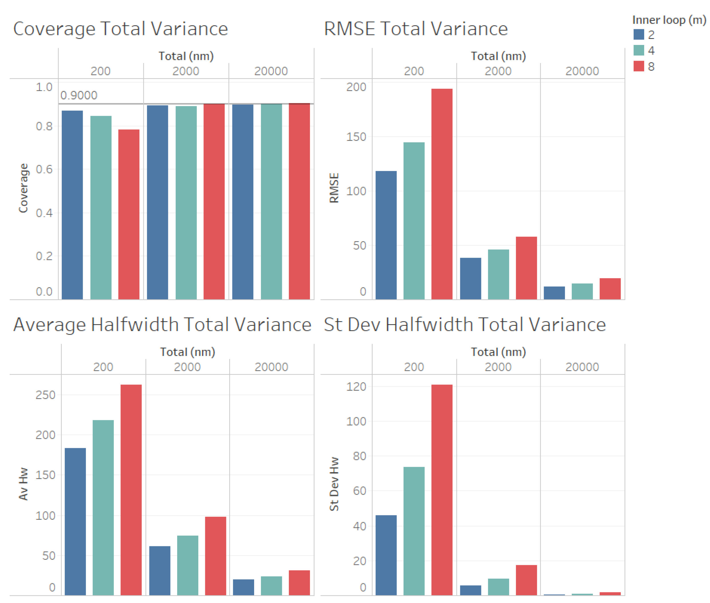
For the estimation of the total variance (illustrated n Figure 5) we obtained similar results for the quality of the estimation as for the estimation of the point forecast , except that a larger values of n is required to obtain reliable coverages. As we observe from Figure 3, the coverages are acceptable (very close to the nominal value of 0.9, for and 10000). These results validate the ACI defined in (6) for the total variance . We also observe from Figure 3 that the RMSE, average halfwidth and standard deviation of halwidths improve (decrease) as the number of observations in the outer level (n) increases, as suggested by Corollary 3. Note also from Figure 5 that a smaller value of m provides smaller RMSE, average halfwidths and standard deviations of halwidths, validating our theoretical results.
Figure 4.
Performance of the estimation of stochastic variance for fixed comparing different values of m.
Figure 4.
Performance of the estimation of stochastic variance for fixed comparing different values of m.
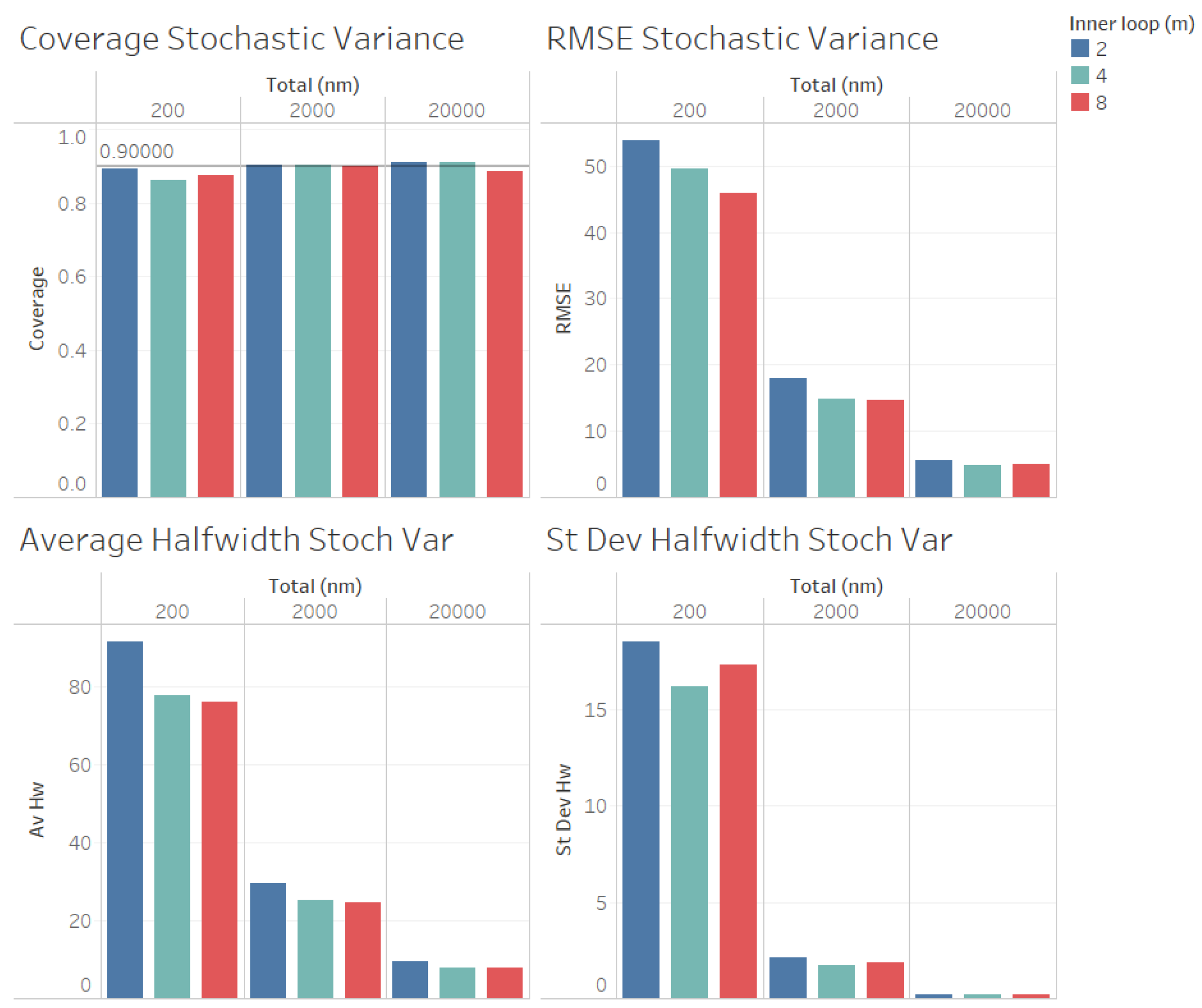
Figure 5.
Performance of the estimation of total variance for fixed comparing different values of m.
Figure 5.
Performance of the estimation of total variance for fixed comparing different values of m.
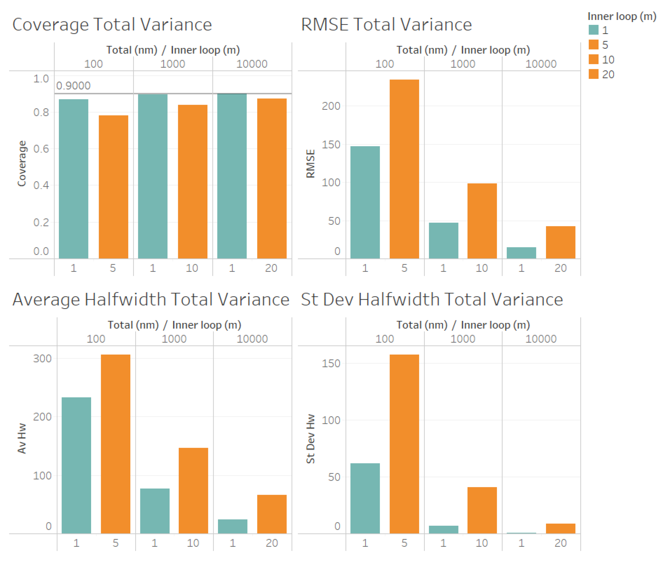
In a second set of experiments we considered , with and for each value of , to compare the quality of the estimation procedures using the value of m that we suggest as optimal for the estimation of point forecast with the value of m suggested in [6] as an adequate choice for m in the case of biased estimators in the inner level of the algorithm of Figure 2. The results of this set of experiments are summarized in Figure 6 and Figure 7. Note that we are not considering the estimation of the stochastic variance in this set of experiments because is required to construct an ACI for the stochastic variance . Note also that we considered , , and , and we are using the same color for in Figure 6 and Figure 7.
In Figure 6 we illustrate the performance measures for the quality of the estimation procedure that we obtained for the estimation of the point forecast in our second set of experiments . As we observe from Figure 6, the coverages are acceptable (very close to the nominal value of 0.9, even for ). These results validate the ACI defined in (6) for the point forecast , and the ACI suggested by Proposition 3. We also observe from Figure 6 that the RMSE, average halfwidth and standard deviation of halwidths are worse for , confirming our finding that, for the same number of replications , produces better point estimators for than confirming the result of Proposition 3.
Finally, in Figure 7 we show the results of our second set of experiments for the estimation of the total variance . We found similar resulta as for the case of the estimation of the point forecast , coverages are very good (even for n = 100), and all performance measure for the ACI (RMSE, average and standard deviation of halfwidths) are worse for , suggesting that, for the same number of replications , produces better point estimators for than .
5. Conclusions
In this paper, we propose methodologies to calculate point estimators (and their corresponding halfwidths), for both the point forecast and the variance components in two-level nested stochastic simulation experiments, for the case where the observations at both levels of the algorithm are independent. These methods can be applied to the construction of Bayesian forecasts based on experiments using a simulation model under parameter uncertainty.
Both our theoretical and our experimental results confirm that the proposed point estimators and their corresponding halfwidths are asymptotically valid, i.e., the point estimators converge to the corresponding parameter values and the halfwidths converge to the nominal coverage as the number of replications (n) of the outer level increases.
Furthermore, given a fixed number of total observations (), we show that the choice of only one replication in the inner level () provides more accurate estimators for both the point forecast (), and the variance of the point forecast (). However, is required for the estimation of .
Directions for future research on this topic includes experimentation with other point estimators, such as, quasi Monte Carlo or Simpson integration, with the objective of finding more accurate point estimators for the parameters considered in this paper.
Funding
This research was supported by the Asociación Mexicana de Cultura A.C. and the National Council of Science of Technology of Mexico under Award Number 1200/158/2022.
Data Availability Statement
The raw data corresponding to our experiments are available in the repository of AppliedMath.
Conflicts of Interest
The Author declare no conflict of interest.
Appendix A
For completeness, we first write three well known theorems. Proofs of Theorem A1 and Theorem A2 can be found, e.g., in [5], and a proof of Theorem A3 can be found, e.g., in [9]. In what follows, we write ⇒ for weak converge (as without explicit mention).
Theorem A1. (Slutsky). Let be random variables and c be a real constant. If , and , then:
- (i)
- (ii)
- (iii)
- , if
Theorem A2. (Continuous mapping). Let be -valued random vectors, and let be a function such that , where is not continuous at , then .
Theorem A3. (Delta method). Let be -valued random vectors, and let g: be a function that is differentiable in a vecinity of . If there exists a matrix G such that the TLC
is satisfied, where , and denotes a (k -variate) normal distribution with mean 0 and variance I (the identity), then
where .
Proof of Corollary 1.
Since are i.i.d. with , it follows from the Law of Large Numbers that . Therefore, by taking for in Theorem A2, we have , so that . Finally, by taking in Theorem A1, it follows from Proposition 2 that
Similarly, since are i.i.d. with , it follows from Theorem A1 and Proposition 2 that
□
Proof of Lemma 1.
Let , , , then the TLC of Theorem A3 is satisfied for
By taking , we have , , and
Then, it follows from Theorem A3 that
and the final conclusion follows from Theorem A1. □
Proof of Proposition 3.
In this proof we follow the notation of Lindeberg-Feller Theorem as in Theorem 7.2.1 of [3].
For n = 1, 2, ..., let and . Then are independent, and for we also have that are independent.
Then if , we have and , so that given there exists such that .
Therefore, given , for we have
so that (1) of Theorem 7.2.1 of [14] is satisfied, and it follows from this Theorem that , where
□
References
- Muñoz, D.F. Simulation output analysis for risk assessment and mitigation. In Multi-Criteria Decision Analysis for Risk Assessment and Management; Ren, J., Ed.; Springer: Heidelberg, Germany, 2021. [Google Scholar]
- Smith, J.S.; Sturrock, D.T. Simio and Simulation: Modeling, Analysis, Aplications, 6th ed.; Simio LLC: Sewickley, Pennsylvania, 2022. [Google Scholar]
- Chung, K.L. A Course in Probability Theory; Academic Press: Cambridge, Massachusetts, 2001. [Google Scholar]
- Asmussen, S.; Glynn, P.W. Stochastic Simulation Algorithms and Analysis; Springer: Heidelberg, Germany, 2007. [Google Scholar]
- Serfling, R.J. Approximation Theorems of Mathematical Statistics; John Wiley & Sons: Hoboken, New Jersey, 2009. [Google Scholar]
- Andradóttir, S.; Glynn, P.W. Computing bayesian means using simulation. ACM TOMACS 2016, 26, paper–10. [Google Scholar] [CrossRef]
- L’Ecuyer, P. Quasi-Monte Carlo methods with applications in finance. Finance and Stochastics 2009, 13, 307–349. [Google Scholar] [CrossRef]
- Zouaoui, F. , Wilson J.R. Accounting for parameter uncertainty in simulation input modeling. IIE Transactions 2003, 35, 781–792. [Google Scholar] [CrossRef]
- Muñoz, D.F.; Glynn, P.W. A batch means methodology for estimation of a nonlinear function of a steady-state mean. Manag Sci 1997, 43, 1121–1135. [Google Scholar] [CrossRef]
- Muñoz, D.F.; Muñoz, D.F. Bayesian forecasting of spare parts using simulation. In Service Parts Management: Demand Forecasting and Inventory Control; Altay, N., Litteral, L.A., Eds.; Springer: Heidelberg, Germany, 2011. [Google Scholar]
- Muñoz, D.F. Estimation of expectations in two-level nested simulation experiments. In Proceedings of the Name of the 29th European Modeling and Simulation Symposium, Barcelona, Spain, 18–20 Sep 2017; 233-238. [Google Scholar]
- Russo, D.; Van Roy, B. Learning to optimize via posterior sampling. Mathematics of Operations Research 2014, 39, 1221–1243. [Google Scholar] [CrossRef]
- Muñoz, D.F.; Muñoz, D.F.; Ramírez-López, A. On the incorporation of parameter uncertainty for inventory management using simulation. International Transactions in Operational Research 2013, 20, 493–513. [Google Scholar] [CrossRef]
Figure 1.
Algorithm for the method of independent replications with parameter fixed at the value .
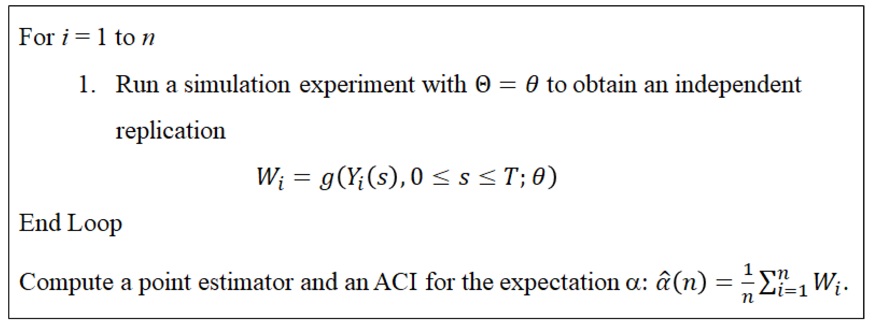
Figure 2.
Two-level algorithm for calculating a point estimator using stochastic simulation under parameter uncertainty.
Figure 2.
Two-level algorithm for calculating a point estimator using stochastic simulation under parameter uncertainty.
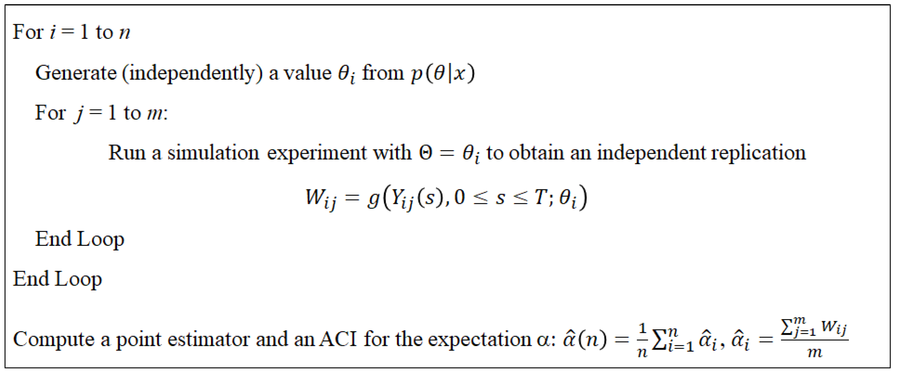
Figure 3.
Performance of the estimation of point forecast for fixed comparing different values of m.
Figure 3.
Performance of the estimation of point forecast for fixed comparing different values of m.
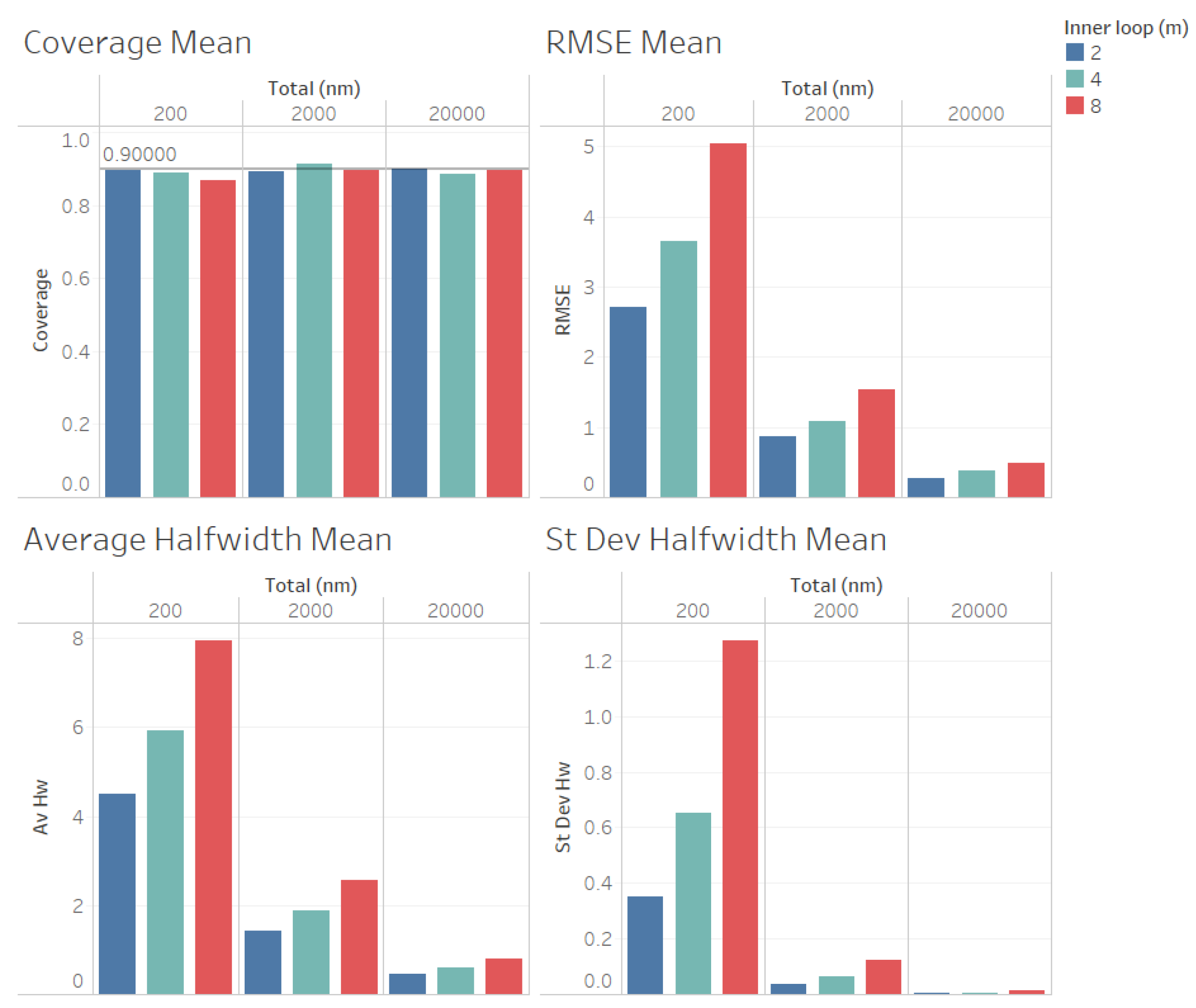
Figure 6.
Performance of the estimation of point forecast for fixed comparing and .
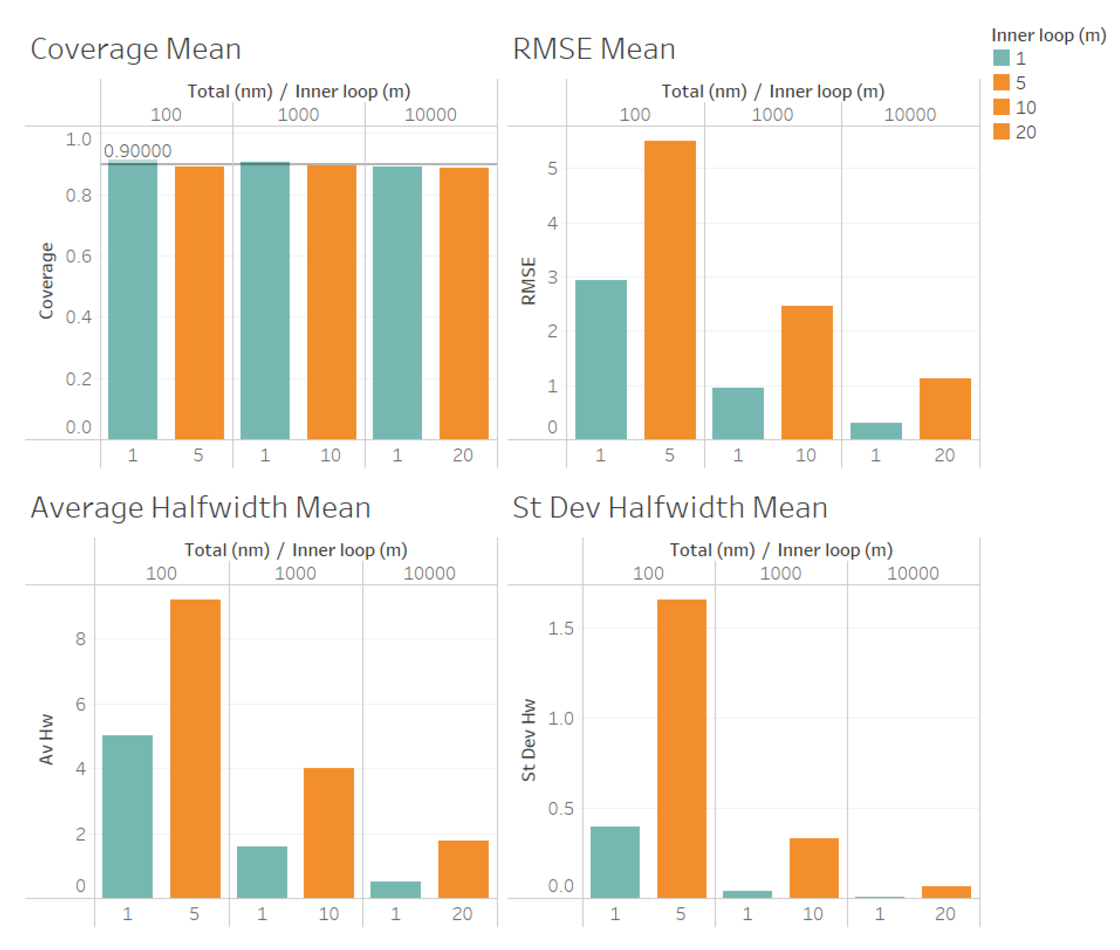
Figure 7.
Performance of the estimation of total variance for fixed comparing and .
Disclaimer/Publisher’s Note: The statements, opinions and data contained in all publications are solely those of the individual author(s) and contributor(s) and not of MDPI and/or the editor(s). MDPI and/or the editor(s) disclaim responsibility for any injury to people or property resulting from any ideas, methods, instructions or products referred to in the content. |
© 2023 by the authors. Licensee MDPI, Basel, Switzerland. This article is an open access article distributed under the terms and conditions of the Creative Commons Attribution (CC BY) license (http://creativecommons.org/licenses/by/4.0/).
Copyright: This open access article is published under a Creative Commons CC BY 4.0 license, which permit the free download, distribution, and reuse, provided that the author and preprint are cited in any reuse.


