

Submitted:
08 May 2023
Posted:
09 May 2023
You are already at the latest version
Abstract
This study presents the solution of the second type of a two-dimensional nonlinear integral
equation in Banach space. Also, the existence and uniqueness of this equation’s solution are
discussed. We utilize a numerical approach involving hybrid and block-pulse functions to obtain
the approximate solution of a two-dimensional nonlinear integral equation. Nonlinear integral
equation in two dimensions is reduced numerically to a system of nonlinear algebraic equations
that can be solved using numerical methods. This study focuses on showing the convergence
analysis for the numerical approach and obtaining an error estimate. Some numerical examples
have been provided to demonstrate the approach’s viability and efficacy
Keywords:
Two- dimensional nonlinear integral equation
; Banach fixed point theorem
; Block-pulse function
; Hybrid functions
; Legendre polynomials
MSC: 41A30; 45G10; 46B45; 65R20
1. Introduction
Integral equations are used in many disciplines of applied mathematics to explore and solve problems. See [1,5,6,10,24,26,27] for more information on the topics of two-dimensional nonlinear integral equations, which have long been of growing interest in many fields, including medicine, biology, physics, geography, and fuzzy control. According to the references [2,3,7,9,10,11,12], many problems in engineering, applied mathematics, and mathematical physics can be reduced into two-dimensional nonlinear integral equations. The analytical solutions to these equations are typically difficult. Therefore, it is necessary to find approximations. For example, Bernstein polynomials hybrid with functions of block-pulse form [4,22] and Legendre hybrid with functions of block-pulse form [13,21] have both recently been examined as computational approaches for solving two-dimensional nonlinear integral equations. Electrical engineering was originally introduced to block-pulse functions by Harmuth, after which additional academics discussed the topic [8].
Recently, hybrid functions have been considered for solving numerous mathematical models, including [20,23,25]. Combining Legendre polynomials and block-pulse functions yields one of these functions. Using block-pulse functions and Legendre polynomials, [18] described a method for solving mixed-type Hammerstein integral equations, whereas [17] proposed a method for solving optimal control of Volterra integral systems. These hybrid functions have also been applied to solving nonlinear Fredholm-Hammerstein systems. [14,30] obtained a numerical solution of partial differential equations with nonlocal integral conditions; [19] solved Fredholm integral equation of the first kind; [28] discovered the optimal solution of linear time-delay systems; [29] discovered the numerical solutions of stochastic Volterra-Fredholm integral equations; and [13] includes the necessary definitions as well as some properties of Legendre polynomials and hybrid block-pulse functions.
In this study, the second type of two-dimensional nonlinear integral is considered. Under special conditions, the Banach fixed point theorem is used to discuss and prove the existence of a unique solution to two-dimensional nonlinear integral equations. We discuss the properties of hybrid functions, which combine block-pulse functions and Legendre polynomials. These integral equations are solved based on some useful properties of hybrid functions. This technique’s major characteristic is its ability to transform an integral problem into a set of algebraic equations; as a result, the solution processes are correspondingly either reduced or simplified.
The article’s structure is as follows: : In Section 2, the existence and unique solution of Eq. (1) are discussed. Section 3 describes a method for estimating a two-dimensional nonlinear integral equation’s solution. The convergence analysis of the provided method is derived in Section 4, Numerical results are shown in Section 5, and conclusion and Remarks are presented in the last Section 6.
This study aims to present a numerical approach for solving the following two-dimensional nonlinear integral equation approximatively:
where are constant scalers having several physical meanings, the function is unknown in the Banach space The kernels are continuous in the same space and the known function is continuous in the space . In addition the constant defines the kind of two- dimensional nonlinear integral equations.
2. Existence of a unique solution for the integral equation
The existence of a unique solution of problem (1) will be discussed and proved in this section using the Banach fixed point theorem. For this, we write Eq. (1) in the form of an integral operator:
where
Also, we assume the following conditions:
- (i)
- The kernels and satisfy the conditions: where and are two constants, assume .
- (ii)
- is a constant.
- (iii)
- The function satisfies the following conditions:
- (iv)
- The function is bounded and satisfy:
Theorem 1.
Assume that the conditions are satisfied. Eq. (1) has an unique solution in the space, . If the condition
is true.
The following two lemmas are necessary for the theorem’s proof:
Lemma 1.
Under the conditions , and , the operator defined by Eq. (2) maps the space into itself.
Proof. In light of formulas (2) and (3), we obtain
Using conditions (i) and (ii), we get
Given conditions and , the above inequality takes on the following form:
where
, so that last inequality becomes
since
According to this inequality, the operator maps the ball into itself, where
since, , therefore we have . Furthermore, lower bounds for the operators V and are involved in the inequality (5).
Lemma 2.
If the conditions , and are verified, then the operator defined by Eq. (2) is continuous in the space .
Proof. For the continuity, Given two functions and in the space and satisfy Eq. (2), then
applying the properties of the norm, we obtain
In view of the conditions (i), (iii-b), and (iv-b), the above inequality becomes
since
This inequality shows that, is a continuous operator in . Moreover is a contraction operator under the condition .
3. Method of solution for the main problem
This section applies the collocation method, two-dimensional hybrid functions, and the Gauss quadrature formula to transform the integral equation (1) into nonlinear systems of equations. The following results are obtained by expanding the function in Eq. (1) in relation to two-dimensional hybrid functions:
where the finite series in equation (6) can be written as
where and are the unknown hybrid coefficients to be determined.
Substituting Eq. (7) into Eq. (1) yields
Now, we discretize Eq. (8) at the set of collocation nodes for as follows:
where
and
The integral operators in Eq. (9) are approximated using the Gauss-Legendre quadrature formula. For this, we use the following transformations to convert the integrals over into the integral over , respectively
The integral over must also be changed into the integral over , having the following form
Then Eq. (9) is converted to
The above equation can be expressed as follows using Gauss-Legendre quadrature:
and and are the corresponding weights.
This technique can be used to transform the two-dimensional nonlinear integral problem (1) into a solvable nonlinear system of algebraic equations.
4. Convergence analysis
The aim of this section is to describe the uniform convergence of the hybrid functions expansion and to determine the maximum absolute truncation error of the function based on hybrid functions.
Theorem 2.
If , then the function converges uniformly to the infinite sum of the hybrid functions of described by (6)
Proof. The hybrid coefficients are defined as
Now, suppose that and , therefore
Using the technique of integration by parts with regard to ℑ and , we obtain
Once again, an integration by parts of above relation, results that
Now, we have
where
Similarly, changing the variable for y as where and integrating by parts with respect to ℘, we get
where
Using the chain derivatives and , it follows that
However
Using the Legendre polynomials’ orthogonality property, we determine that
thus
and
By substituting (13) and (14) into (11), we obtain
Therefore, the series is absolutely convergent. Also,
and the series (6) converges to the function uniformly.
Theorem 3.
The maximum absolute truncation error of the series solution (6) to two- dimensional nonlinear integral equation is estimated to be,
Proof.
Using the hybrid functions’ orthogonality property and taking relation (15) into consideration, we are able to
5. Application and numerical results
In order to show the accuracy and efficiency of the proposed method, some numerical examples are given in this section. We introduce the following notation to study the absolute values of this method’s errors:
where and are the exact solution and the approximate solution of the integral equations, respectively.
Example 5.1.
Consider the following two- dimensional nonlinear integral equation:
where
The exact solution is Using the proposed numerical technique, where and in the interval .
Example 5.2.
Consider the nonlinear integral equation:
where
The exact solution is Using the presented numerical technique with and in the interval .
6. Conclusions and Remarks
The following can be deduced from the above analysis and discussion:
- Under some conditions, the equation (1) has a unique solution in the space .
- After applying the proposed method, a two-dimensional integral equation of the second kind, in time and position, tends to result in an algebraic system of equations.
- A nonlinear system of algebraic equations has a solution.
- Maximum error obtained by proposed method is decreasing when number of is increasing.
- Illustrative examples are provided to evaluate and validate the effectiveness and dependability of the proposed method.
References
- Abdou, M.A.; Soliman, A.A.; Abdel–Aty, M.A. On a discussion of Volterra–Fredholm integral equation with discontinuous kernel. J. Egypt Math. Soc. 2020, 28. [Google Scholar] [CrossRef]
- Abdou, M.A.; Nasr, M.E.; Abdel-Aty, M.A. A study of normality and continuity for mixed integral equations. J. of Fixed Point Theory Appl. 2018, 20. [Google Scholar] [CrossRef]
- Al-Bugami, A.M. Numerical treating of mixed Integral equation two-dimensional in surface cracks in finite layers of materials. Advanced in math. Physics 2022, 25, 1–12. [Google Scholar] [CrossRef]
- Alipour, M.; Baleanu, D.; Babaei, F. Hybrid Bernstein block-pulse functions method for second kind integral equations with convergence analysis. Abstr. Appl. Anal. 2014, 2014, 1–8. [Google Scholar] [CrossRef]
- Bakhshayesh, S.J. , Discontinuous Galerkin approximations for Volterra integral equations of the first kind with convolution kernel. Indian Journal of Science and Technology 2015, 8, 1–4. [Google Scholar] [CrossRef]
- Brezinski, C.; Redivo-Zalglia, M. Extrapolation methods for the numerical solution of nonlinear Fredholm integral equations. J. Integral Equations Appl. 2019, 31, 29–57. [Google Scholar] [CrossRef]
- Chen, Z.; Jiang, W. An Efficient Algorithm for Solving Nonlinear Volterra-Fredholm Integral Equations. Appl. Math. Comput. 2015, 259, 614–619. [Google Scholar] [CrossRef]
- Datta, K.B.; Mohan, B.M. Orthogonal Function in Systems and Control, 9, World Scientific, 1995.
- Elzaki, T.M.; Alamri, A.S. Note on new homotopy perturbation method for solving nonlinear integral equations. J. Math. Comput. Sci. 2016, 6, 149–155. [Google Scholar]
- Golberg, M.A.; Chen, C.S. Discrete Projection Methods for Integral Equation Computational Mechanics Publications, 1997.
- Gouyandeh, Z.; Allahviranloo, T.; Armand, A. Numerical Solution of Nonlinear Volterra-Fredholm-Hammerstein Integral Equations via Tau-Collocation Method With Convergence Analysis. J. Comput. Appl. Math. 2016, 308, 435–446. [Google Scholar] [CrossRef]
- Hafez, R.M.; Youssri, Y.H. Spectral Legendre-Chebyshev treatment of 2D linear and nonlinear mixed Volterra-Fredholm integral equation. Math. Sci. Lett. 2020, 9, 37–47. [Google Scholar]
- Hashemzadeh, E.; Maleknejad, K.; Basirat, B. Hybrid functions approach for the nonlinear Volterra–Fredholm integral equations. Proc. Comput. Sci. 2011, 3, 1189–1194. [Google Scholar] [CrossRef]
- Hesameddini, E.; Riahi, M. Hybrid Legendre Block-pulse functions method for solving partial differential equations with non-local integral boundary conditions. J. Inf. Optim. Sci. 2019, 40, 1391–1403. [Google Scholar] [CrossRef]
- Katani, R. Numerical solution of the Fredholm integral equations with a quadrature method. SeMA J. 2019, 76, 449–452. [Google Scholar] [CrossRef]
- Kreyszig, E. Introductory Functional Analysis with Applications, John Wiley and Sons. Inc., New York, 1989.
- Maleknejad, K.; Ebrahimzadeh, A. An efficient hybrid pseudo-spectral method for solving optimal control of Volterra integral systems. Math. Commun. 2014, 19, 417–435. [Google Scholar]
- Maleknejad, K.; Hashemizadeh, E. Numerical solution of the dynamic model of a chemical reactor by hybrid functions. Procedia. Comput. Sci. 2011, 3, 908–912. [Google Scholar] [CrossRef]
- Maleknejad, K.; Saeedipoor, E. An efficient method based on hybrid functions for Fredholm integral equation of the first kind with convergence analysis. Appl. Math. Comput. 2017, 304, 93–102. [Google Scholar] [CrossRef]
- Mashayekhi, S.; Razzaghi, M. Numerical solution of distributed order fractional differential equations by hybrid functions. J. Comput. Phys. 2016, 315, 169–181. [Google Scholar] [CrossRef]
- Marzban, H.R.; Tabrizidooz, H.R.; Razzaghi, M. A composite collection method for the nonlinear mixed Volterra–Fredholm–Hammerstein integral equation, Commun. Nonlinear Sci. Numer. Simul. 2011, 16, 1186–1194. [Google Scholar] [CrossRef]
- Masouri, Z. Numerical expansion-iterative method for solving second kind Volterra and Fredholm integral equations using block-pulse functions, Adv. Comput. Tech. Electromagn. 2021, 20, 7–17. [Google Scholar]
- Mirzaee, F.; Alipour, S.; Samadyar, N. Numerical solution based on hybrid of Block-pulse and parabolic functions for solving a system of nonlinear stochastic Ito-Volterra integral equations of fractional order. J. Comput. Appl. Math. 2019, 349, 157–171. [Google Scholar] [CrossRef]
- Mirzaee, F. Numerical solution of system of linear integral equations via improvement of block-pulse functions. J. Math. Model. 2016, 4, 133–159. [Google Scholar]
- Mohammadi, F.; Moradi, L.; Baleanu, D.; Jajarmi, A. A hybrid functions numerical scheme for fractional optimal control problems: Application to non analytic dynamic systems. J. Vib. Control. 2017, 24, 5030–5043. [Google Scholar] [CrossRef]
- Nasr, M.E.; Abdel-Aty, M.A. Analytical discussion for the mixed integral equations. J. of Fixed Point Theory Appl. 2018, 20. [Google Scholar] [CrossRef]
- Nasr, M.E.; Abdel-Aty, M.A. A new techniques applied to Volterra–Fredholm integral equations with discontinuous kernel. J. of Computational Analysis and Appl. 2021, 29, 11–24. [Google Scholar]
- Rafiei, Z.; Kafash, B.; Karbasi, S.M. State-control parameterization method based on using hybrid functions of Block-pulse and Legendre polynomials for optimal control of linear time delay systems. Appl. Math. Model. 2017, 45, 1008–1019. [Google Scholar] [CrossRef]
- Ray, S.S.; Singh, S. Numerical solution of stochastic Volterra-Fredholm integral equations by hybrid Legendre Block-pulse functions. Int. J. Nonlinear Sci. Numer. Simul. 2018, 19, 1–9. [Google Scholar]
- Sahu, P.K.; Ray, S.S. Hybrid Legendre Block-pulse functions for the numerical solutions of system of nonlinear Fredholm-Hammerstein integral equations. Appl. Math. Comput. 2015, 270, 871–878. [Google Scholar] [CrossRef]
- Wang, K.; Wang, Q. Taylor polynomial method and error estimation for a kind of mixed Volterra-Fredholm integral equations. Appl. Math. Comput. 2014, 229, 53–59. [Google Scholar] [CrossRef]
Figure 1.
Exact and approximate solution of Eq. (16) with and
Figure 1.
Exact and approximate solution of Eq. (16) with and
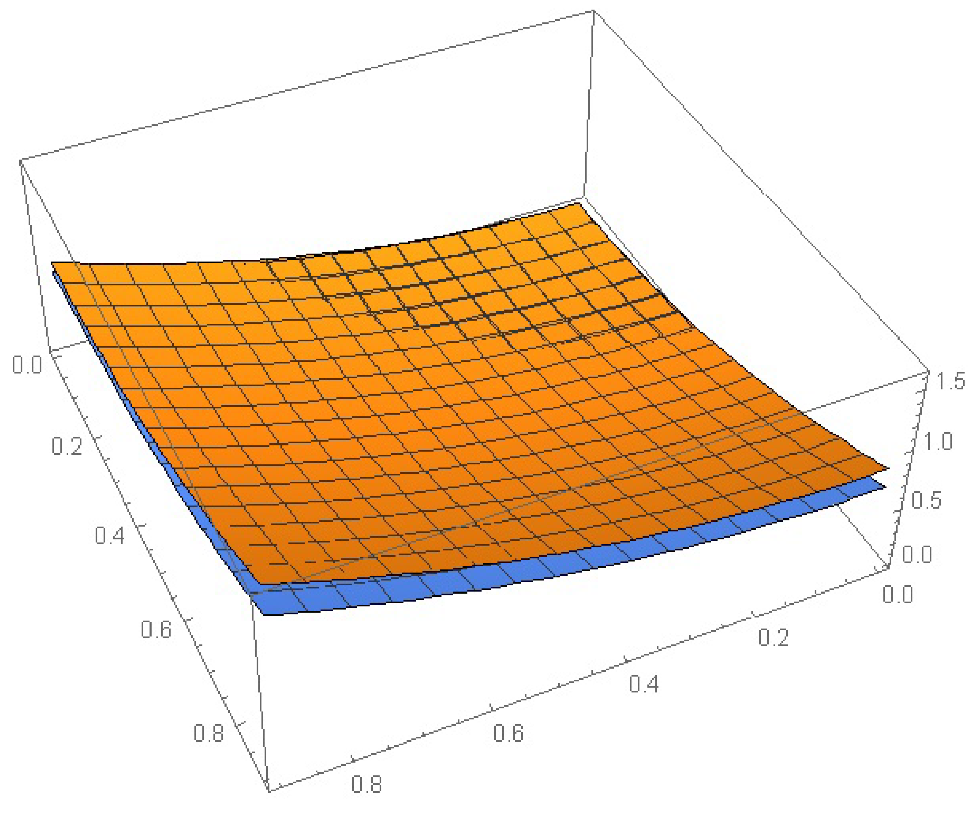
Figure 2.
Exact and approximate solution of Eq. (16) with and
Figure 2.
Exact and approximate solution of Eq. (16) with and
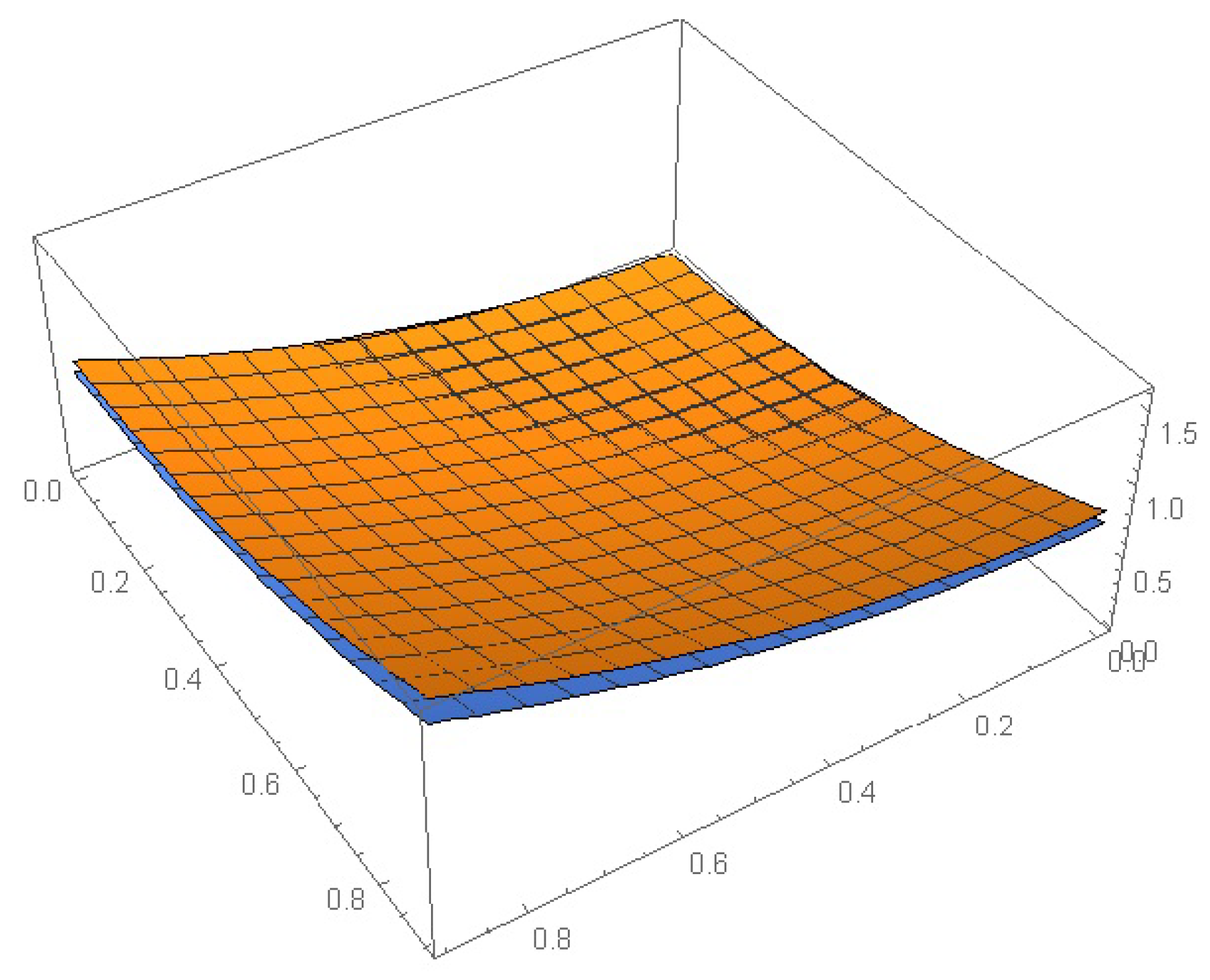
Figure 3.
Exact and approximate solution of Eq. (16) with and
Figure 3.
Exact and approximate solution of Eq. (16) with and
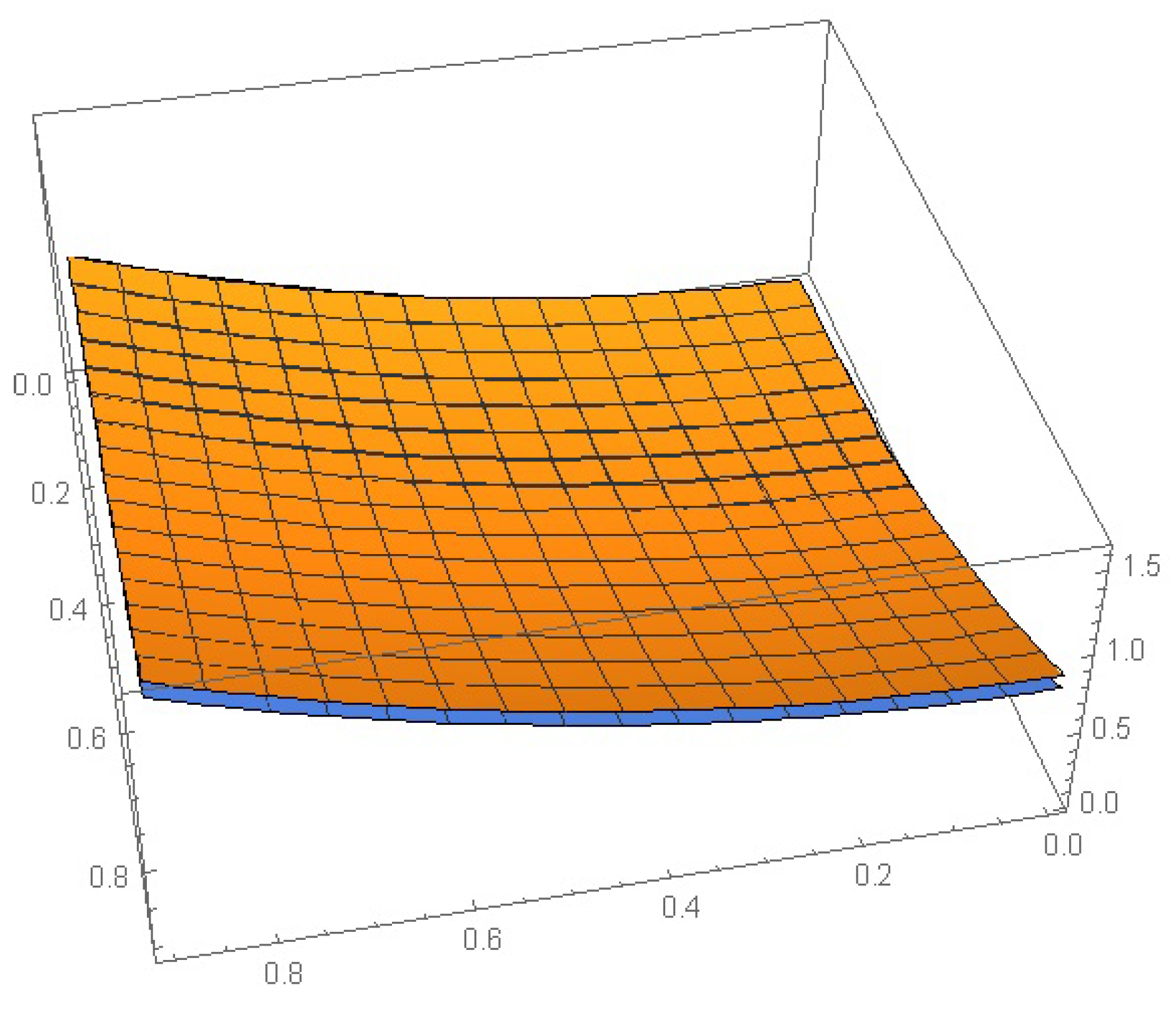
Figure 4.
Exact and approximate solution of Eq. (16) with and
Figure 4.
Exact and approximate solution of Eq. (16) with and
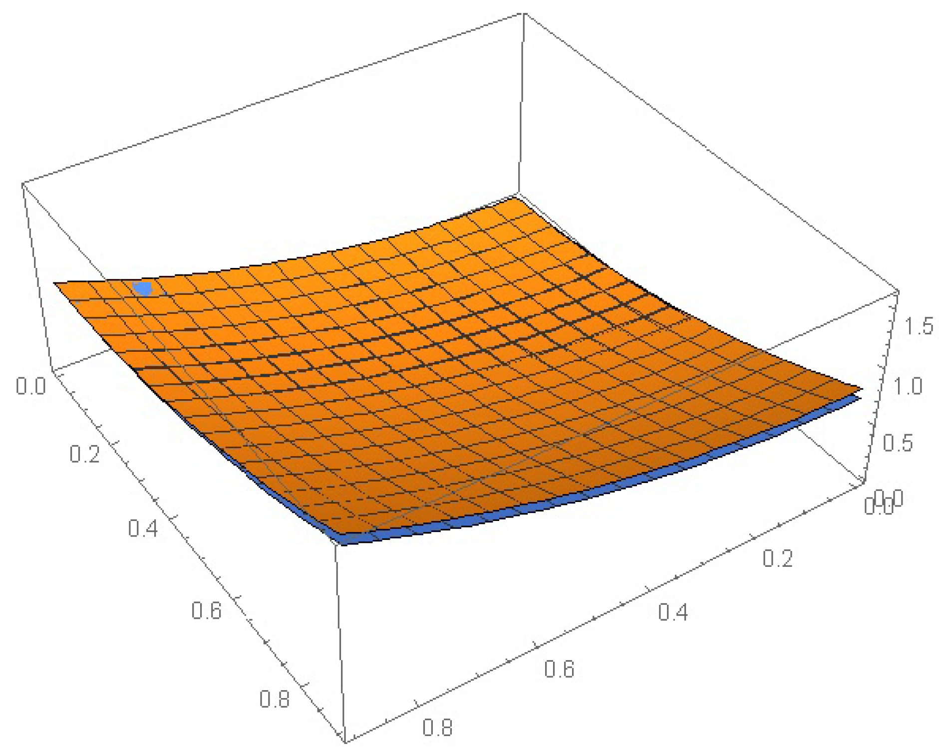
Figure 5.
Exact and approximate solution of Eq. (17) with and
Figure 5.
Exact and approximate solution of Eq. (17) with and
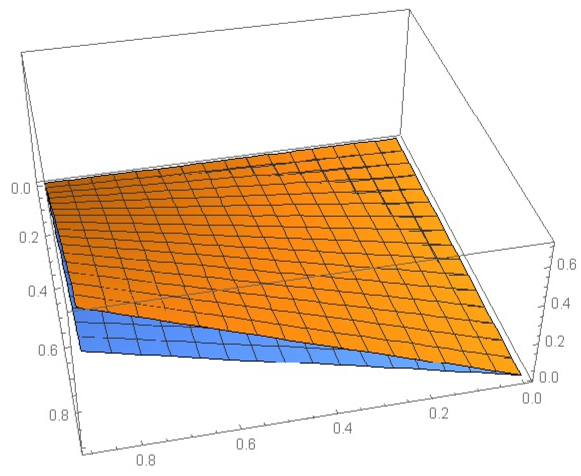
Figure 6.
Exact and approximate solution of Eq. (17) with and
Figure 6.
Exact and approximate solution of Eq. (17) with and
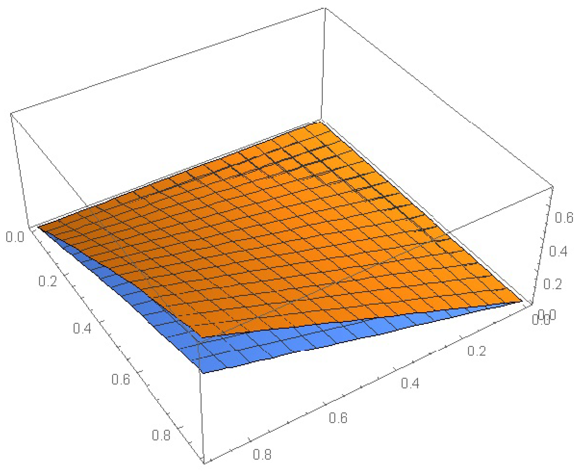
Figure 7.
Exact and approximate solution of Eq. (17) with and
Figure 7.
Exact and approximate solution of Eq. (17) with and
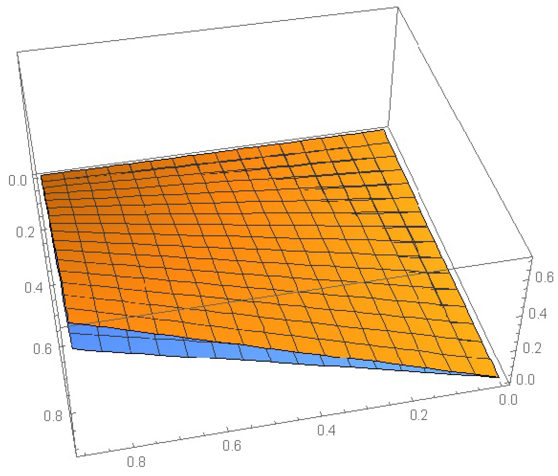
Figure 8.
Exact and approximate solution of Eq. (17) with and
Figure 8.
Exact and approximate solution of Eq. (17) with and
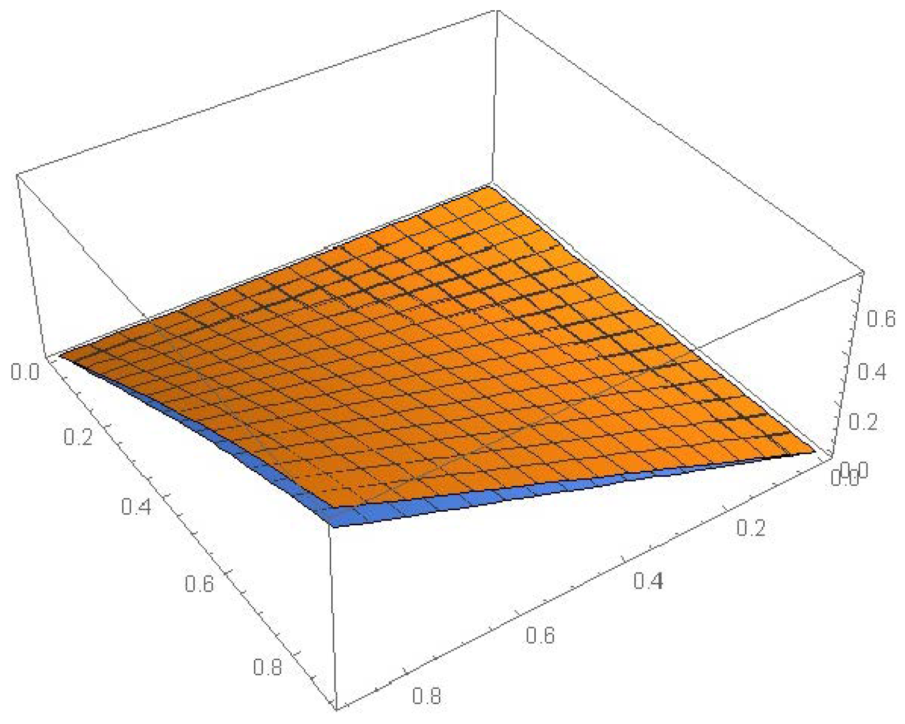

Table 1.
Absolute error of solution of Eq. (16) by using present method with and .
Table 1.
Absolute error of solution of Eq. (16) by using present method with and .
| (0,0) | 5.62845 | 3.25447 | 2.36512 | 1.32654 |
| (0.1,0.1) | 2.51405 | 2.36524 | 1.36524 | 6.32514 |
| (0.2,0.2) | 5.62103 | 2.36985 | 5.36214 | 8.22551 |
| (0.3,0.3) | 2.02154 | 3.58412 | 8.32541 | 6.32165 |
| (0.4,0.4) | 4.58721 | 3.65413 | 2.21345 | 1.32114 |
| (0.5,0.5) | 7.36212 | 2.23651 | 3.65221 | 2.36985 |
| (0.6,0.6) | 1.36521 | 1.65214 | 7.32651 | 2.92541 |
| (0.7,0.7) | 5.26512 | 1.36524 | 6.32541 | 6.32548 |
| (0.8,0.8) | 5.62514 | 4.36210 | 8.36251 | 7.32614 |
| (0.9,0.9) | 5.65214 | 6.25489 | 5.32658 | 1.36524 |
Table 2.
The maximum error for different values of and for Eq (16).
Table 2.
The maximum error for different values of and for Eq (16).
| 6.2103 | 6.53210 | 5.32658 | 1.36524 |
Table 3.
Absolute error of solution of Eq. (17) by using present method with and .
Table 3.
Absolute error of solution of Eq. (17) by using present method with and .
| (0,0) | 3.20514 | 5.32641 | 6.32141 | 2.36541 |
| (0.1,0.1) | 3.25481 | 9.32541 | 5.32187 | 3.65874 |
| (0.2,0.2) | 3.32541 | 3.21554 | 2.36414 | 7.36584 |
| (0.3,0.3) | 4.32641 | 5.32654 | 5.32684 | 3.36241 |
| (0.4,0.4) | 5.36854 | 6.36524 | 8.32546 | 6.32584 |
| (0.5,0.5) | 6.93154 | 7.1.365 | 6.32541 | 8.65241 |
| (0.6,0.6) | 1.32511 | 3.21547 | 9.99215 | 4.32516 |
| (0.7,0.7) | 4.32658 | 4.36561 | 1.32154 | 8.69854 |
| (0.8,0.8) | 5.32666 | 5.76524 | 2.34541 | 4.36215 |
| (0.9,0.9) | 6.32541 | 7.96525 | 3.25456 | 1.05214 |
Table 4.
The maximum error for different values of and for Eq (17).
Table 4.
The maximum error for different values of and for Eq (17).
| 6.32541 | 7.96525 | 3.25456 | 1.05214 |
Disclaimer/Publisher’s Note: The statements, opinions and data contained in all publications are solely those of the individual author(s) and contributor(s) and not of MDPI and/or the editor(s). MDPI and/or the editor(s) disclaim responsibility for any injury to people or property resulting from any ideas, methods, instructions or products referred to in the content. |
© 2023 by the authors. Licensee MDPI, Basel, Switzerland. This article is an open access article distributed under the terms and conditions of the Creative Commons Attribution (CC BY) license (http://creativecommons.org/licenses/by/4.0/).
Copyright: This open access article is published under a Creative Commons CC BY 4.0 license, which permit the free download, distribution, and reuse, provided that the author and preprint are cited in any reuse.