Submitted:
08 May 2023
Posted:
09 May 2023
You are already at the latest version
Abstract
In this study we propose a semi-parametric, parsimonious Value at Risk forecasting model, based on quantile regression and machine learning methods, combined with readily available market prices of option contracts from the over-the-counter foreign exchange rate interbank market. We aim at improving existing methods for VaR prediction of currency investments using machine learning. We employ two different methods - ensemble methods and neural networks.
Explanatory variables are implied volatilities with plausible economic interpretation. The forward-looking nature of the model, achieved by the application of implied volatilities as risk factors, ensures that new information is rapidly reflected in Value at Risk estimates. To the best of our knowledge, this paper is the first to utilize information in the volatility surface, combined with machine learning and quantile regression, for VaR prediction of currency investments.
The proposed ensemble models achieve good estimates across all quantiles. The light gra-dient-boosting machine model and the categorical boosting model both yield estimates which are better than, or equal to, those of the benchmark model. The neural network models are in general quite unstable.
Keywords:
Value at Risk
; over-the-counter foreign exhange (OTC FX) options
; quantile regression
; Machine Learning (ML)
1. Introduction
The ability to model Value at Risk (VaR) with high accuracy is an important tool for quantifying risk in financial markets (Schaumburg (2012)). VaR is an estimate of the loss that will be exceeded with a small probability during a fixed holding period. In addition to occupying a prominent role in regulatory frameworks, VaR will continue to be important for financial institutions as a measure of market risk.
This paper extents the work of de Lange et al. (2022) As noted by the authors, machine learning models might further improve their predictions as such models can handle non-linearities among explanatory variables. The contribution of this study is employing different machine learning models and techniques to improve VaR predictions of currency investments, compared to the benchmark Quantile Regression Implied Moments (QR-IM) model.
We employ both neural networks and ensemble methods for VaR predictions. For this purpose, recurrent neural network (RNN) and long short-term memory neural network (LSTM )stand out among the neural network models. Both these models appear to yield more accurate forecasting results for time series data compared to the feed forward networks, which however are still widely used. Amidst the ensemble methods, the random forest model is the most frequently used. Gradient boosting methods have also been used, but less commonly. Ensemble methods and neural networks are considered state of the art models in the machine learning community today. We test gradient boosting methods as well as random forest alongside recurrent neural networks, long short-term memory neural networks and feed forward networks. The various models are created using different model architectures as well as hyperparameter tuning, and model stacking for the ensemble models.
We examine several options for tuning and improving the two concepts of ensemble methods and neural networks. In addition, the training and validation data sets are constructed using the QR-IM model. This model was proposed by de Lange et al. (2022) for forecasting Value-at-Risk in currency markets. All models are trained with the same data and validated on the same out-of-sample period.
To the best of our knowledge, this paper is the first to utilize information in the volatility surface, more precisely at-the-money volatility and risk reversals as proxies for higher order moments, combined with machine learning and quantile regression to provide accurate VaR estimates.
Our main findings are:
- The LightGBM model and the Categorical boost model yield more accurate VaR estimates than the benchmark QR-IM model.
- The ensemble models achieve good estimates across all quantiles.
- The neural network models are in general quite unstable and could benefit from more training data and perhaps a better model architecture.
- Model stacking and hyperparameter tuning improved overall model predictions.
The remainder of this paper is organized as follows: Section 2 provides an overview of the literature, section 3 presents the data, section 4 describes the methodology, section 5 presents and discusses results and section 6 concludes.
2. Literature Review
Quantile regression methods are often applied to Value at Risk forecasting. Engle and Manganelli (1999) proposed the CAViaR method. This model can directly estimate quantiles instead of modelling the whole distribution. Taylor (2008) proposed the exponentially weighted quantile regression (EWQR) model for estimating Value at Risk. He found that this model outperformed both GARCH-based methods and CAViaR models. Chen and Chen (2005) find that calculating VaR at the Nikkei 225 index using quantile regression outperforms the conventional variance-covariance approach.
A few papers have applied quantile regression in the context of forecasting volatility or VaR of foreign exhange rates. Taylor (1999) finds that a quantile regression approach provides a better fit to multi-period data when forecasting volatility compared to variations of the GARCH(1,1) model. Huang et al. (2011) use quantile regression to forecast foreign exchange rate volatility. Jeon & Taylor (2013) include implied volatility as an additional regressor in CAViaR models and obtain increased precision of FX VaR estimates.
Effective explanatory variables are essential to make accurate forecasts of Value at Risk for currency crosses. Chang et al. (2013) provides an outline of different forecasting objectives using options data, including option-implied individual moments. Barone-Adesi et al. (2019) and Huggenberger et al. (2018) show how to use options data to compute forward looking VaR and Conditional-VaR measures. The information content of option combinations - such as risk reversal - has been studied in the context or arbitrage-free option pricing and hedging in papers by Bossen et al. (2010) and Sarma et al. (2003). de Lange et al. (2022) forecast Value-at-Risk in foreign exchange markets using OTC at-the-money option contracts from foreign exchange interbank market to model volatility, and risk reversals as a proxy for higher order moments. Their QR-IM model outperforms benchmark models like GARCH and CAViaR-SAV for VaR forecasts.
A number of previous studies has confirmed the forecasting ability of a plain vanilla feed forward neural network over traditional statistical models. However, standard neural networks have limitations. Most notably, these models rely on the assumption of independent data observations, which presents a problem when data points are related through time. In order to overcome this problem, Bijelic and Ouijjane (2019) use a Gated Recurrent Unit type of neural network to produce one-step-ahead volatility forecasts of the EURUSD exchange rate. Their model is outperformed by a GARCH(1,1) model for the VaR 95%. Xu et al. (2021) modelled Value-at-Risk of foreign exchange rates with three different neural network models; the deep belief network (DBN), multilayer perceptron (MLP), and long short-term memory network. Other studies that apply neural networks for predicting foreign exchange rates are Yaya Heryadi and Antoni Wibowo, (2021) and He et al. (2018).
Neural networks have been used in a vast variety of studies trying to model Value at Risk. Petneházi (2021) uses convolutional neural networks to forecast Value at Risk. Modifying the algorithm slightly, the convolutional networks can estimate arbitrary quantiles of the distribution, not only the mean, thus allowing the network to be applied to VaR-forecasting. Pradeepkumar and Ravi (2017) forecast financial times series volatility using a developed particle swarm optimization trained quantile regression neural network, named SPOQRNN. They compare this model to three traditional forecasting models including GARCH, multilayer perceptron, general regression neural network and random forest, finding that the SPOQRNN outperformed the other models.
A few authors have used Artificial Neural Network (ANN) for forecasting Value at Risk. Taylor [20] applied a quantile regression neural network approach to estimate the conditional density of multiperiod returns. The model is compared to GARCH-based quantile estimates on daily exchange rates. Xu et al. (2016) developed a new quantile autoregression neural network (QARNN) model based on an artificial neural network architecture. By optimizing an approximate error function and standard gradient-based optimization algorithms, QARNN outputs conditional quantile functions recursively. This allows the QARNN to explore non-linearity in financial time series. Yen et al. (2009) used ANN to forecast VaR on a stock index. The authors stated that the model benefit from adding more exogenous parameters in the estimation process, such as interest rates.
Yan et al. (2015) use long short-term memory neural networks in a quantile regression framework to learn the tail behavior of financial asset returns. Their model captures both the time-varying characteristic and the asymmetrical heavy-tail property of financial time series. The authors combine the sequential neural network with a self-constructed parametric quantile function to represent the conditional distribution of asset returns. Kakade et al. (2022) propose a hybrid model that combines LSTM and a bidirectional LSTM with GARCH, to forecast volatility. The model is evaluated on periods with extreme volatility, the 2007-09 global financial crisis and the covid recession of 2020–2021. The proposed model provides significant improvement in the quality and accuracy of VaR forecasts compared to benchmark GARCH models.
Ensemble methods have been used by a number of studies estimating VaR. Andreani et al. (2022) introduced the use of mixed-frequency variables in a quantile regression framework by merging the Quantile Regression Forest algorithm and the Mixed-Data-Sampling model. The empirical application of the model delivered adequate VaR forecasts and outperformed popular existing models used in VaR forecasting, such as the GARCH model, in terms of quantile loss. Jiang et al. (2017) proposed a hybrid semi-parametric quantile regression random forest approach to evaluate Value at Risk. The model was used to explain the non-linear relationship in multi-period VaR measurement. Görgen et al. (2022) used a generalized random forest (GRF) for predicting Value-at-Risk for cryptocurrencies. They found that random forest outperformed quantile regression methods, including GARCH-type and CAViaR models, when tailored to conditional quantiles. The authors state that the adaptive non-linear form of GRF appears to capture time-variations of volatility and spike-behavior in cryptocurrency return especially well, in contrast to more conventional financial econometric methods. Gradient boosting methods were tested by Cai et al. (2020) for modeling VaR. They found the method to be effective at capturing risk.
3. Data
We apply our ensemble- and neural network models to empirical data for the EURUSD spot exchange rate, taking implied volatility quotes as input data, examining the models’ predictive properties. Daily exchange rates and implied volatility quotes are sourced from Bloomberg, covering the period from 2009:01 to 2020:12.
3.1. Spot-rate returns
The daily returns are calculated as , where is the spot exchange rate at time t. In our case, this is the daily return of a dollar measured in euros. Table 1 displays descriptive statistics for daily log-returns from 2009:01 to 2020:12 and Figure 1 plots the time series correspondingly. The return series exhibit the stylized facts that have been widely documented in the financial economics literature; with unconditional means close to zero, clustering of volatility and fat-tailed return distributions.
3.2. Examining the data
Figure 2 displays time series for at-the-money volatilities (ATM) and 25–delta risk reversals (RR) for European EURUSD options with one week to expiry and reveals the stochastic nature of the volatility surface. ATM levels have spiked around important economic events, such as the Brexit vote in June 2016 and the Covid 19 outbreak in March 2020. Panel (c) shows that the sign of the RR has changed over time and taken both positive and negative values, which in itself is an interesting observation. If the risk reversal reflects the relative probability of depreciation and appreciation of a currency, time-varying sign and magnitude of the risk reversal can be interpreted as an indication of time varying probability of tail events. Panels (b) and (d) display empirical distributions, which are skewed and leptokurtic for both variables. ATM volatility is naturally bounded below by zero, but spikes during periods of market turmoil which causes a heavy right tail. The risk reversal displays a highly non-normal, heavy-tailed empirical distribution.
3.3. Testing the data set
In order to test the data for stationarity we performed an augmented Dickey-Fuller unit root test and conclude that our data is stationary. Further to rule out multicollinearity, we ran a variance inflation factor test, or VIF in short. No sign of multicollinearity was discovered. We also tested our data for heteroskedasticity using the Breusch-Pagan test and serial correlation between the explanatory variables using a Breusch-Godfrey test. The Breusch-Pagan test indicated some sign of heteroskedasticity, whereas no sign of serial correlation was found.
4. Methods
In this section, we provide a brief outline of the models we have used to produce our VaR forecast. We demonstrate how the data set is generated, briefly and generically explain the QR-IM model, ensemble methods and neural networks. We also provide a short note on prepossessing of data and implementation of models. A subsection is devoted to the specific ensemble models and neural networks, which we have implemented on our data.
4.1. Generating the training data
In order to examine the different machine learning methods, we need to create a proper data set containing the required quantiles. In this study we use two methods for creating the training data set. First, we employ the methods proposed by de Lange et al. (2022) using the QR-IM model. Our second approach is using gradient boosting to generate quantiles based on the generated predictions. This is achieved by the light gradient boosting-machine model and the gradient boosting model. Both models have built-in options for quantile regression. The QR-IM is explained below.
4.1.1. The quantile regression implied moments model
de Lange et al. (2022) propose a quantile regression implied moments (QR-IM) model. We employ this model for generating benchmark, in sample quantiles for our currency data. The model is based on the hypothesis that the volatility surface of OTC FX options contains information, which can be utilized to improve the accuracy of VaR estimates. Similar to de Lange et al. (2022), we study data for at-the-money (ATM) options and risk reversals (RR).
At-the-money options are struck at the FX forward rate. ATM options have an initial delta of 50%. The ATM implied volatility is the risk-neutral expectation of spot rate volatility over the remaining life of the option.
Risk reversals involve the simultaneous sale of a put option and purchase of a call option. The two options are struck at the same delta. At the outset a 25% delta risk reversal will have a combined delta of 50% and very little sensitivity to gamma and vega because of the offsetting effect of the long and short position. Risk reversals are usually quoted as the difference in implied volatility of similar call and put options with the equal delta. The risk reversal reflects the difference in the demand for out-of-the money options at high strikes compared to low strikes. Thus, it can be interpreted as a market-based measure of skewness, the most likely direction of the spot movement over the expiry period.
In the general case, the simple linear quantile regression model is given by:
where the distribution of is left unspecified. The expression for the conditional q quantile, 0 < q < 1, is defined as any solution to the minimization problem:
Where
In the QR-IM model, the conditional quantile
function can be expressed as
A unique vector of regression parameters can be obtained for each quantile of interest, and
the whole return distribution can be found, given observed values for the
at-the-money volatility (ATM) and the risk reversal (RR).
4.2. Value-at-Risk
VaR is a statistical risk measure of potential
losses and summarizes in a single number the worst loss over a target horizon
that will not be exceeded with a given level of confidence. Formally, the VaR
at a level of the profit and loss distribution X is
defines as:
The most common methods for calculating VaR are usually divided into parametric, semi-parametric and nonparametric approaches.
4.3. Ensemble learning
In this study we employ two base methods for estimating VaR - ensemble learning and neural networks. Ensemble learning is the process of using multiple models, often called weak learners, trained over the same data and combined to obtain better results. Weak learners, or base models, are models that on average perform slightly better than random chance. This is either because they have a high bias or because they have too much variance to be robust. The idea of ensemble methods is to attempt reducing bias and/or variance of such weak learners by combining several of them to create a strong learner that achieves better performance.
Low bias and low variance are two of the most desirable features of a model. There is also a trade-off between degrees of freedom and the variance of a model. Introducing too many degrees of freedom can cause high variance (bias-variance trade off).
When combining weak learners, we need to assure that our choice of weak learners is consistent with the way we aggregate the models. If we choose base models with low bias but high variance, we should employ an aggregating method that tends to reduce variance and vice versa. In general, there are three major kinds of algorithms that aim at combining weak learners: bagging, boosting and stacking.
Bagging learns homogeneous weak learners independently and combines them following some kind of deterministic averaging process. Boosting, which also often considers homogeneous weak learners, learns them sequentially and combines them following a deterministic strategy. Stacking, learns weak learners in parallel and combines them by training a meta-model which outputs a prediction based on the different weak model predictions. In general, both boosting and stacking mainly try to produce strong models with less bias than their components, whereas bagging mainly focuses on getting an ensemble model with less variance than its components.
4.4. Deep learning
Deep learning refers to machine learning methods using deep neural networks to approximate some unknown function based only on inputs and expected outputs. Below we briefly explain the concepts of artificial neural networks including some activation functions relevant to this study. Furthermore, the learning process of the neural network will be explained along with optimizers and the concept of batch and epoch.
4.4.1. Artificial neural network (ANN)
ANNs hereafter referred to as neural networks (NNs), recognize underlying relationships in a data set through a process that mimics the way the human brain operates. NNs are non-linear functional approximators that can be tuned to approximate an unknown function based on observations and target outputs. NNs are structured in consecutive layers. Each layer takes an input, applies a transformation, and returns an output. The perception, originally described by Rosenblatt (1958), acts as the inspiration for the neuron, the foundational building piece of the layer. There is an associated weight for each element in the input vector to the neuron. The bias of the neuron can optionally be added to the input. The neuron then determines an output by adding the inputs and the weights assigned to each input: An arbitrary positive number of neurons that each provide an output can make up a layer in an NN. Input can be a vector of size m and output a vector of size n, equal to the number of neurons in the layer. Calculating the output vector involves multiplying the input vector by the weight matrix of the layer:
Where x is the input vector, y is the output vector, W is a m × n matrix containing the weights for the n neurons in the layer and b is the vector of biases.
4.4.2. Activation functions
As mentioned in Section 4.4.1, neural networks are organized in successive layers, each layer computes an output given an input as described in Equation (7). The output of one layer is then subjected to a nonlinear transformation before being passed as input to the following layer. This is referred to as an activation function. Commonly used activation functions are:
The logistic function
The logistic function, also known as the sigmoid activation function, transforms the values into the range [0,1]:
Tanh
The hyperbolic tangent function, simply referred to
as tanh, is similar to the sigmoid activation function, but instead output
values in the range [−1, 1]:
ReLU
The Rectified Linear Unit (ReLU) activation function outputs values in the range [0,1⟩. It does this by taking the maximum of the input and zero:
All mentioned activation functions are displayed in Figure 3, in blue, with their derivatives in yellow.
4.5. Implementation
We use Keras to construct the neural network, which serves as an interface for the TensorFlow library. TensorFlow was developed by Google and is both a free and open-source library for machine learning. Keras offers both ordinary neural network layers, recurrent-layers and LSTM-layers, in addition to a multitude of different machine learning methods.
4.6. The chosen ensemble models
According to the literature review in Section 2, the random forest algorithm was more frequently employed to estimate VaR compared to the gradient boosting methods. Therefore, in this study we tested different gradient boosting methods, as well as the random forest, for predicting VaR.
Random forest
The random forest model is an ensemble of many weak learners, in this case decision trees. It can be applied to classification and regression problems. The regression procedure using random forest starts by splitting of features and then creates decision trees. Every tree makes its individual decision based on the data. The average value predictions from all trees becomes the final prediction.
Gradient boosting
Gradient boosting on decision trees is a form of machine learning that works by progressively training more complex models to maximize the accuracy of predictions. Gradient boosting is particularly useful for predictive models that analyze ordered (continuous) data and categorical data. Gradient boosting benefits from training on huge data sets. Gradient boosting is one of the most efficient ways to build ensemble models. The combination of gradient boosting with decision trees provides state-of-the-art results in many applications with structured data.
Extreme gradient boosting
Extreme gradient boosting (XGBoost) is an improved version of the gradient boosting algorithm. This algorithm creates decision trees sequentially. Different weights are assigned to all the independent variables, which are then fed into the decision tree that predicts results. The weight of wrongly predicted variables by the tree is increased and the variables are then fed to the second decision tree. This is known as a gready algorithm. These individual classifiers/predictors then ensemble to give a strong and more precise model. This works for regression, classification, ranking, and user-defined prediction problems.
Light gradient boosting-machine
Light gradient boosting machine, known as LightGBM, is a gradient lifting framework which is based on the decision tree algorithm. It can be used in classification, regression, and many more machine learning tasks. Compared to XGBoost it splits leaf-wise and chooses the maximum delta value to grow, rather than level-wise. LightGBM has a great advantage when performing hyperparameter optimization. This is because the different input-parameters are easily controlled.
Category boosting
Categorigal boosting, in short CatBoost, provides a way of performing classifications and rankings of data by using a collection of decision-making mechanisms. Results generated by the learners are weighted and classified based on the strengths and weaknesses of each learner.
4.7. Hyperparameter architecture
The hyperparameter tuning is a little different for the ensemble methods and neural networks. Nevertheless, the general aim is to minimize the loss function and maximize accuracy while reducing bias and overfitting. For both the ensemble methods and the neural networks, choosing the correct architecture is non-trivial. When it comes to the ensemble methods, the chosen architecture is mostly based on the method in use, whether this is ordinary random forest or some gradient boost technique. Choosing a method also restricts a lot of the possible tuning. In this study, the process of hyperparameter tuning for the ensemble methods has been carried out by the use of software (if it exists), and trial and error. Typically, the tuning parameters are the number of leaves, number of trees and the learning rate.
In a neural network there are a lot of possible variations. The hyperparameters that need to be adjusted in the neural network are the number of layers, number of nodes in each layer, the lookback period, activation functions, learning rate, bach size and number of epochs. This has been achieved through an iterative approach, optimizing one parameter at a time.
Another possibility for tuning the models is the training and validation period. The training data consists of data from 2009-07-07 to 2017-12-29. For the neural network there is also the training period. We have split the training period 80/20 percent, into the neural network training set and the test set respectively. The validation set is equal for both periods and consists of data from 2018-01-03 to 2020-09-25. Too short a training set can make the data prone to outliers, however it may be less overfitted. Too long a training period makes the data prone to overfitting, and the model may be useless for its actual task. This is because one cannot test the model on enough data to detect anomalies in the model.
A neural network needs many input parameters to find any type of patterns in the data. In our data there are only two parameters. That may be too few for a neural network to work properly. Thus, a third parameter has been created. This is an interaction term between the two already existing parameters.
4.8. The considered neural networks
In this study we employ the recurrent neural network, the long-short-term memory and the feed forward neural network.
Feed forward neural network
The feed forward neural network (FFNN) is an artificial neural network. Connections between the nodes do not form any type of cycle. The information is passed only in one direction through the hidden nodes to the output nodes. Feed Forward Neural Networks with a single hidden layer is the most widely used neural network for forecasting (Zang, 1998).
Recurrent neural network
A recurrent neural network (RNN) is a class of artificial neural networks where connections between nodes can create a cycle, allowing output from some nodes to affect subsequent input to the same nodes.
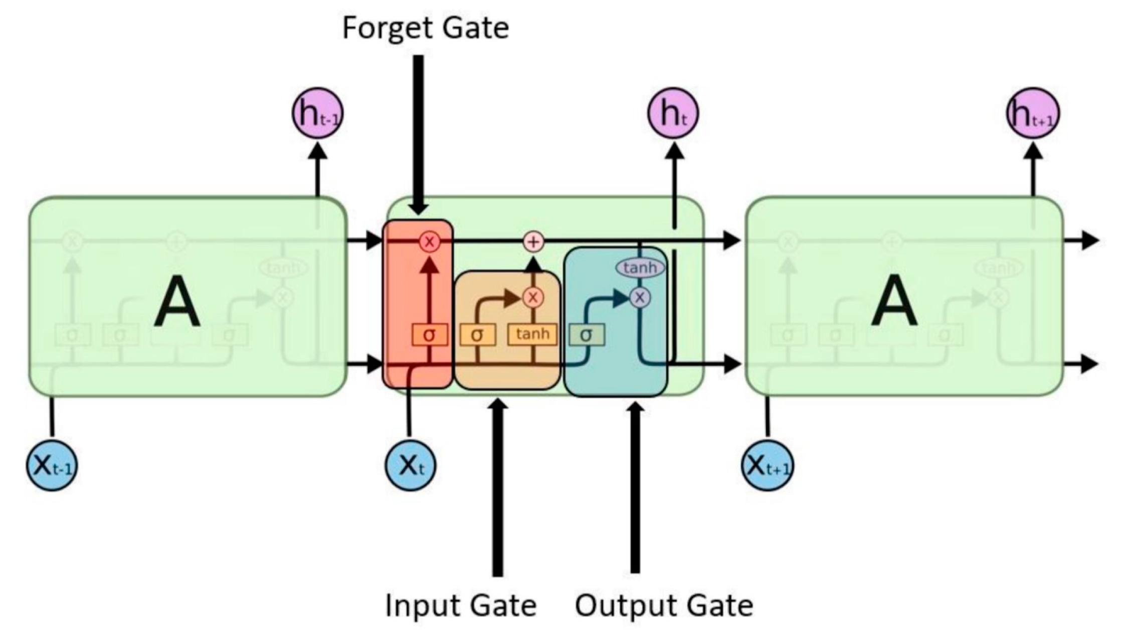
Long short-term memory
The long short-term memory (LSTM) can consolidate information from far in the past with that which is more recent. A forget gate, an input gate, and an output gate make up the LSTM-cell. While the gates govern the information flow in and out of the cell, the fundamental function of the LSTM-cell is to recall information over time intervals. The gates essentially decide which information is remembered and which is forgotten. The information that the LSTM-cell remembers is kept in its cell state and computed based on the input . The results of the previous output is kept in the forget gate.
Figure 4.
A long short term memory layer.
4.9. Explainable AI
We introduce Shapley values to enhance comprehension of how the machine learning models operate. Shapley (Shap) values originate from Game Theory and are frequently used for post-hoc model explainability in machine learning models. The idea is to see the impact each feature has on the target. For further explanation see the original paper by Shapley (1951).
4.10. Developed neural network models
For all models, a batch size of 5 has been used. Each model was allowed to run for 120 epochs, but the final number varied based on whether early stopping was activated. All models had their weights randomly initialized and used the Adam optimizer.
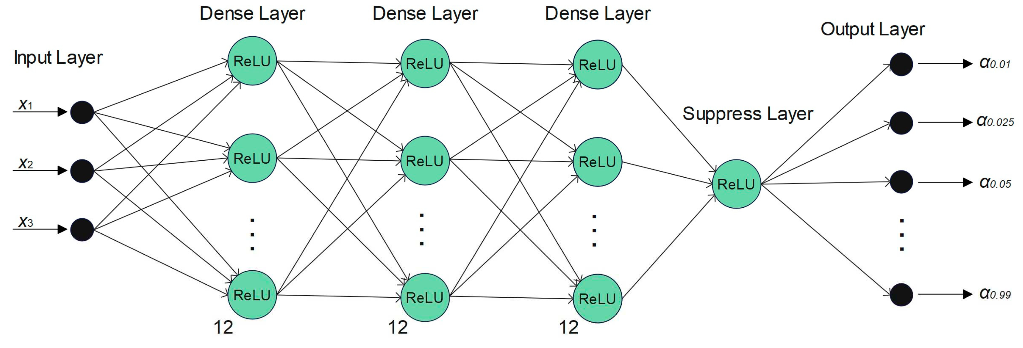
4.10.1. Feed forward neural network
The feed forward neural network has three dense layers consisting of 12 nodes, and a dropout frequency of 0.2. After the three dense layers comes a suppress layer, with a dropout frequency of 0.2. This layer suppresses the data and make the predictions more stable. All layers have a ReLU activation function. The model output are the predicted quantiles: α: [0.01, 0.025, 0.05, 0.95, 0.975, 0.99].
Figure 5.
The feed forward neural network used in this study.
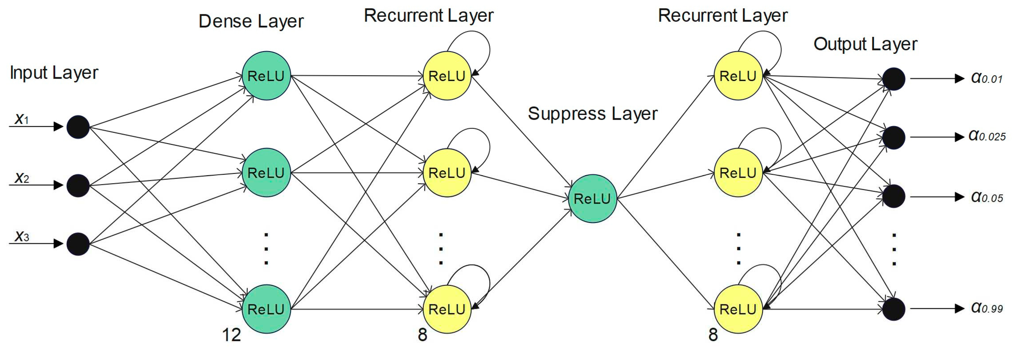
4.10.1. Recurrent neural network
The recurrent neural network has two dense layers consisting of 12 nodes and between them a recurrent layer consisting of 8 nodes. All layers have dropout frequencies of 0.2 and a ReLU activation function. The model output is the predicted quantiles: α: [0.01, 0.025, 0.05, 0.95, 0.975, 0.99].
Figure 6.
The recurrent neural network used in this study.
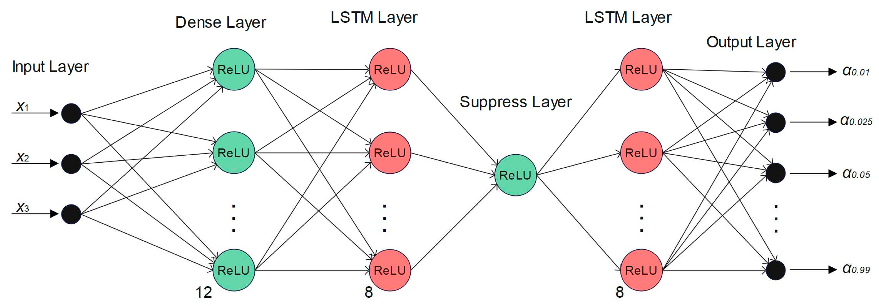
4.10.1. Long short-term memory neural network
The LSTM neural network starts with a dense layer of 12 nodes, followed by an LSTM layer with 8 nodes. Then comes a suppress layer consisting of one node needed to make the model more stable, followed by a LSTM layer with 8 nodes. All layers have dropout frequencies of 0.2 and a ReLU activation function. Outputs from the model are the predicted quantiles: α: [0.01, 0.025, 0.05, 0.95, 0.975, 0.99].
Figure 7.
The LSTM neural network used in this thesis.
4.11. Evaluating the models
We let denote the indicator function, i.e., a function which returns 1 if the event A occurs and 0 if not, represented by (11). The true return is given by while the predicted return (VaR estimate) is given by . provides the total number of predictions. We introduce the following metrics with this notation, which are used to examine superiority among the VaR models:
If the VaR is specified at confidence level α the
breach level should roughly be equivalent to α. The Breach ratio is
given as:
Calculating the nominal breach of the model over the total number of predictions is one method of evaluating performance. The model with smaller Sum if breach is favored given models with comparable breach ratios since this would suggest that the model is at least closer to the true value of the loss. The Sum if breach is given as:
It is also interesting to know how close a prediction is to the predicted medium when no breach occurs. Thus, the Sum if no breach is given as:
Both formulas are expressed for the higher quantiles. The same formulas, however, can be used for the lower quantiles. In addition, the following 4 metrics are used for further comparison:
5. Results
In this section we present results. Throughout all estimates, a fixed training window from July 1, 2009 to December 31, 2017 is used, and the out-of-sample period covers January 1, 2018 to September 28, 2020.
5.1. Estimating the quantile regression VaR model
Table 2 displays the estimated quantile regression coefficients for the ATM variables and the 25 delta RR variables. The model is estimated on daily Bloomberg data during the in-sample period (2009:07-2017:12). The coefficients are scaled by 100 for readability. As for the sign, magnitude, shape, and statistical significance of regression coefficients, the results are consistent for both the ATM variable and the RR variable.
The breach ratios of the estimated quantiles of the in-sample data are also shown in Table 2. The breach ratio displays good coverage throughout the data with respect to the estimated quantiles, as would be expected as the coefficients are statistically significant.
Figure 8.
Quantile regression coefficients QR-IM.
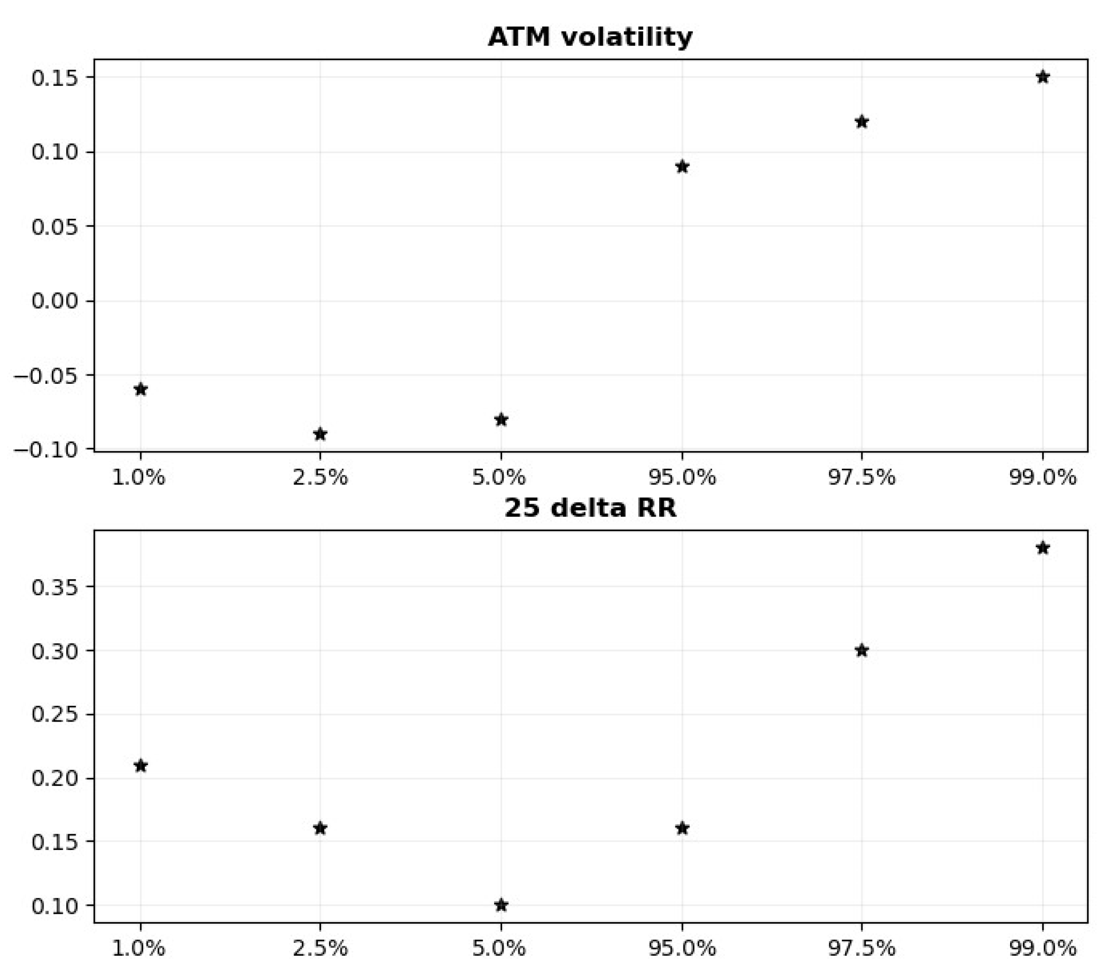
The estimated ATM coefficients support the view that the ATM is an indicator of overall market risk. The upper panel of figure 8 depicts a nonlinear, increasing relationship between the quantiles and the ATM regression coefficients. The coefficients are projecting the shape of the tails of the conditional return distribution. Observe that the coefficients are negative for the lower quantiles and positive for the higher quantiles. In addition, the absolute value of ATM coefficients is slightly higher in the right tail compared to the left tail. This indicates a non-linear relationship between implied volatility and returns.
The lower panel of figure 8 reveals that the RR coefficients form a U-shaped pattern and that all are positive. This indicates that implied volatility is more important when estimating both ends of the tails. However, since all coefficients are statistically significant, all quantile-estimates of the return distribution will improve from employing implied volatility.
5.2. General scheme for evaluating the machine learning models
We have tested different uses of the algorithms for ensemble models: Random Forest, Extreme Gradient Boosting, Light Gradient Boosting, and Categorical Boosting.
The data has been split in two for training and validation. The training set starts at the beginning of the sample period and lasts until the end of 2017. The validation period starts in 2018 and last until the end of the data set. This part is used for validation and testing the performance of the model. Figure 9 illustrates the concept. To illustrate the scheme in full detail, we present results for the random forrest model in the next section.
5.2.1. Illustrating the scheme: Random Forest
In this section we describe how the random forest algorithm has been tested. The data used in the training originates from the data generated by the QR-IM model in Equation (4), discussed in the previous section. The model is trained individually on each quantile. The in-sample data for RR and ATM volatility, along with the in sample estimated quantiles in Section 5.1, are used for training the model. For testing, only the sampling data for RR and ATM volatility is used. The results are listed in Table 3.
The first thing to notice is the increased performance for estimates of higher-order quantiles; 95%. 97.5% and 99%. Second, the sum if no breach increases further away from the mean. This makes sense as these estimates should be further away from the sampling data compared to quantiles closer to the mean. Third, as expected, the sum if breach decreases towards the tails of the distribution. Fourth, the sum if breach is almost equal to zero at the quantiles in the tails. This suggests that the model yields promising results when predicting spike behavior.
The graph shown in Figure 10 displays all the point-estimates for the different quantiles, produced by the random forest algorithm. One thing to notice is how closely the predictions move in line with the underlying data. This gives a good indication of how well the model works with the EURUSD data.
Figure 11 shows a distribution of the Shap-values calculated from the random forest ensemble method. The plot indicates symmetry in the estimation of the quantiles. Further, risk reversal seems to be the more significant model parameter, as it displays both the greatest density and magnitude in the figure. In this model, high values for the risk reversal provide a positive contribution to the prediction, and low values provide a negative contribution. Excluding outliers in the implied volatility, the high/ low values have the same contribution as seen for the risk reversal.
Basically, we have followed the scheme outlined above for evaluating all our machine learning models. In addition to the random forrest model, we have further tested two XGBoost models, three LightGBM models, one categorical boost (CatBoost) model and three neural networks. We also created a stacking model, combining the LGBM 2 model with the CatBoost model. Stacking (like hyper parameter tuning) is a tool used for improving model performance.
The difference in performance of the two XGBoost models (and the three LightGBM models) stems from the difference in the data sets constructed to train them (Table 4). We have also tested three different neural networks: A feed forward neural network (FFNN), a recurrent neural network (RNN) and a long-short term memory neural network (LTSM). The different data sets used for training the model are summarized in table 4.
To save space we will not report details from examining all models like we did with the Random forrest model above. Instead, we provide a summary comparing the performance of the different models to the QR-IM model, which we have chosen as benchmark for this study.
But first, a brief note on the neural networks:
For training and validation of the neural networks, we have split the data in three parts. The first part starts at the beginning of the data set and lasts until the end of 2017. This part is used for training and testing the model. From the first part 80% of the data is used for training and the remaining for testing. While the second part starts in 2018 and lasts until the end of the data set. This part is used for the model validation. All three periods are illustrated in Figure 12.
5.3. Summary of results - comparing the ML models to the QR-IM model
We validate the out-of-sample performance of the different ML-methods against the QR-IM model developed by de Lange, et al (2022).
In general, the performance of the ensemble methods is more stable and consistent than that of the neural networks. The ensemble methods handle the periods with outliers better than the neural networks, whose predictions tend to explode around these events.
The ensemble models perform well compared to the baseline QR-IM model. Three models stand out in comparison to the baseline model: LightGBM 2, CatBoost, and the stacking model between the two. These models all perform better or equal to that of the QR-IM model on the lower quantiles, 1%, 2.5% and 5%. At the higher quantiles, 95%, 97.5% and 99%, the QR-IM model is better or equal to the three models.
The neural network models are in general quite unstable and is probably not particularly well suited for this task. The models produce worse or equal quantile predictions compared to the QR-IM model for all quantiles.
All models are summarized with their breach ratios for the out of sample data in Table 5.
We note that for the sum if breach parameter, less is better. By having a small sum, the model is better at predicting the outcome when a breach happens. However, if a small sum if breach value is combined with a high value for sum if no breach then the model may be too conservative in its predictions. In Table 6 both the if breach (i.b.) and if no breach (i.n.b.) sums are listed for all models. It is difficult to distinguish between the models and find a superior model. The random forest, XGB model 1 and CatBoost algorithms are all very similar when comparing the i.b. scores, all having an approximate score of 0.17. However, the random forest is significantly better when comparing the i.n.b scores, having the lowest score of 35.91. Thus, the random forest may be considered superior amongst the three. It is more difficult to distinguish between the LBGM 1 and the LGBM 2, each having its one superior trait. Thus, the choice of model depends on which feature sum if breach and sum if no breach one deems more important. The LBGM model 1 has the lowest i.b. score among all models, of 0.164.
In Table 7, all the models are summarized with their Christoffersen test p-values and DQ-test p-values with four lags. Both the XGB model 2 and LightGBM model 3 rejects the null hypotheses. Thus, the observed number of VaR breeches is significantly different from the expected number of breeches for the two models. The remaining models generally display high p-values, indicating high forecasting performance across the quantiles.
6. Conclusion
In this study we employ ensemble methods and neural networks to forecast Value at Risk for daily exchange rates. Our aim is to improve VaR predictions of currency investments compared to a benchmark Quantile Regression Implied Moments (QR-IM) model. The ensemble methods, which are forward-looking and utilizes directly observable option prices as explanatory variables, show great potential at predicting the daily exchange rate. The neural network, though also forward-looking and utilizing directly observable option prices as explanatory variables, does not perform at a desired prediction level.
We emphasize six key outtakes from our study:
- The ensemble methods are better at predicting the spike behavior of the EURUSD than the neural networks. The ensemble methods are well suited for predicting the daily EURUSD currency cross distribution, including its VaR.
- The second LightGBM model, Categorical boost, and the stacking model between the two, stand out in terms of comparing the breach values to the base line, QR-IM, model. These models all perform better or equal to the latter at the lower quantiles and have poorer or equal performance at the higher quantiles.
- The random forest and LightGBM 1 and 2 have the best performances among the stand-alone models, in terms of i.b. and i.n.b. values.
- Neural networks can improve a lot compared to the ensemble methods. One way of doing this might be introducing more layers and more nodes. However, by doing so, the models become more of a black box.
- The advantage of neural networks compared to ensemble methods is the way they estimate the quantiles. The neural network is constructed such that all quantiles can be estimated simultaneously. On the other hand, the ensemble methods forecast one quantile at a time. For huge data sets, the possibility of computing all quantiles simultaneously can significantly improve computational time.
- Model stacking and hyperparameter tuning significantly improved the models in terms of the overall performance of the breach ratio.
6.1. Future research
Several possible directions can be taken to further examine the models explored in this study. The models’ performance should be tested in less efficient markets than the EURUSD. Including more explanatory variables, such as macroeconomic variables, might improve the models. Also, one could try different types of combinations of layers in the neural networks. This should lead to better forecasts and more stable results, at the cost of transparency of these networks. Lastly, ensemble methods might be improved from further exploring hyperparameter tuning and stacking methods.
Author Contributions
Suggesting research problem, P.E.d.L. and M.R., methodology, H.M.B., P.E.d.L. and M.R.; software, H.M.B.; validation, H.M.B.; formal analysis, H.M.B.; data curation, H.M.B. and M.R.; writing—original draft preparation, H.M.B. and P.E.d.L.; writing—review and editing, H.M.B., P.E.d.L. and M.R.; All authors have read and agreed to the published version of the manuscript.
Funding
This research received no external funding.
Data Availability Statement
All data used for this study is publicly available. The authors retrieved the data from Bloomberg.
Conflicts of Interest
The authors declare no conflict of interest.
References
- Andreani, M., Candila V. & Petrella, L. (2022). Quantile Regression Forest for Value-at-Risk Forecasting Via Mixed-Frequency Data. 4th International Conference on Information and Communications Technology (ICOIACT). Springer International Publishing. ISBN: 978-3-030-99638-3.
- Barone-Adesi, G., Legnazzi C. & Sala, C. (2019). Option-implied risk measures: An empirical examination on the s&p 500 index. International Journal of Finance & Economics. Vol. 24, issue 4. [CrossRef]
- Bijelic, A., & Ouijjane, T. (2019). Predicting exchange rate value-at-risk and expected shortfall: A neural network approach. https://lup.lub.lu.se/student-papers/search/publication/8989138.
- Bossens, F., Rayée, G., Skantzos, N. S. & Deelstra, G. (2010). Vanna-volga methods applied to fx derivatives: From theory to market practice. International Journal of Theoretical and Applied Finance. https://arxiv.org/pdf/0904.1074.pdf.
- Cai, X., Yang, Y. & Jiang, G. (2020). Online risk measure estimation via natural gradient boosting. 2020 Winter Simulation Conference. [CrossRef]
- Chang, B. Y., Christoffersen, P. & Jacobs, K. (2013). Market skewness risk and the cross section of stock returns. Journal of Financial Economics, 2013. Vol. 107, issue 1.
- Chen, M. & Chen, J. (2002). Application of quantile regression to estimation of value at risk. Review of Financial Risk Management. https://www.jcic.org.tw/upload/download/7e0d92a1-1d70-48a7-8d21-fee5317e9ce3.pdf.
- de Lange, P. E., Risstad, M., & Westgaard S. (2022). Estimating value-at-risk using quantile regression and implied moments. The Journal of Risk Model Validation. Vol. 16, no. 1.
- Engle, R. F., & Manganelli, S. (2004). Caviar: Conditional autoregressive value at risk by regression quantiles. Journal of Business & Economic Statistics. Vol. 22, no. 4.
- Görgen, K., Meirer, J. and Schienle, M. (2022). Predicting value at risk for cryptocurrencies with generalized random forests. Available at SSRN: https://ssrn.com/abstract=4053537 or. /: at SSRN: https. [CrossRef]
- He, K., Ji, L., Tso, G. K. F., Zhu, B. & Zou, Y. (2018). Forecasting exchange rate value at risk using deep belief network ensemble-based approach. Procedia Computer Science. file:///C:/Users/pelange/Downloads/Forecasting_Exchange_Rate_Value_at_Risk_using_Deep.pdf.
- Heryadi, Y. & Wibowo, A. (2021). Foreign exchange prediction using machine learning approach: A pilot study. International Conference on Information and Communications Technology.
- Huang, A. Y., Peng, S. P., Li, F., & Ke, C. J. (2011). Volatility forecasting of exchange rate by quantile regression. International Review of Economics & Finance. Vol. 20, issue 4.
- Huggenberger, M., Zhang, C. & Zhou, T. (2018). Forward-looking tail risk measures. SSRN papers. file:///C:/Users/pelange/Downloads/SSRN-id2909808.pdf.
- Jeon, J., & Taylor, J. W. (2013). Using CAViaR Models with Implied Volatility for Value-at-Risk Estimation. Journal of Forecasting, 32, 62-74. [CrossRef]
- Jiang, F., Wu, W. & Peng, Z. (2017). A semi-parametric quantile regression random forest approach for evaluating muti-period value at risk. 2017 36th Chinese Control Conference (CCC) [Internet]. 2017 Jul 7;5642–6. Available from: http://resolver.scholarsportal.info/resolve/19341768/v2017inone/5642_asqrrffemvar.xml.
- Kakade, K., Jain, I. & Mishra, A. K. (2022). Value-at-risk forecasting: A hybrid ensemble learning garch-lstm based approach. Resources Policy. Vol. 78.
- Petneházi, G. (2021). Quantile convolutional neural networks for value at risk forecasting. 2021. Machine Learning with Applications. Vol. 6. https://reader.elsevier.com/reader/sd/pii/S2666827021000487?token=4F25CEBCCE1C55F298694A71EB8700AF046FA8EC25CE9943280D97AF6446930D3A0C09FD8D495980B6F8041037869800&originRegion=eu-west-1&originCreation=20230426095056.
- Pradeepkumar, P. & Ravi, V. (2017). Forecasting financial time series volatility using particle swarm optimization trained quantile regression neural network. Applied Soft Computing. Vol. 58.
- Rosenblatt, F. (1958). The perceptron - a perceiving and recognizing automaton. https://blogs.umass.edu/brain-wars/files/2016/03/rosenblatt-1957.pdf.
- Sarma, M., Thomas, S. & Shah, A. (2003). Selection of value-at-risk models. Journal of Forecasting.
- Schaumburg, J. (2012). Predicting extreme value at risk: Nonparametric quantile regression with refinements from extreme value theory’, Computational Statistics and Data Analysis.
- Shapley, L. S. (1951) Notes on the n-person game – ii: The value of an n-person game. https://www.rand.org/content/dam/rand/pubs/research_memoranda/2008/RM670.pdf.
- Taylor, J. W. (2008). Using exponentially weighted quantile regression to estimate value at risk and expected shortfall, Journal of financial Econometrics. Vol 6, issue 3.
- Taylor, J. W. (1999). A quantile regression approach to estimating the distribution of multiperiod returns. Journal of Derivatives. Vol. 7, no. 1.
- Taylor, J. W. (2000). A quantile regression neural network approach to estimating the conditional density of multiperiod returns. Journal of Forecasting. Vol. 19, issue 4.
- Xu, Z., Zeng, Y., Xue, Y. & Yang, S. (2021). Foreign exchange prediction using machine learning approach: A pilot study. 2021 4th International Conference on Information and Communications Technology (ICOIACT). file:///C:/Users/pelange/Downloads/1570751055final.pdf.
- Xu, Q., Liu, X., Jiang, C. & Yu, K. (2016). Quantile autoregression neural network model with applications to evaluating value at risk. Applied Soft Computing. Vol. 49. https://www.tarjomefa.com/wp-content/uploads/2017/05/6615-English-TarjomeFa.pdf.
- Yan, X., Zhang, W., Ma, L., Liu, W. & Wu, Q. (2015). Parsimonious quantile regression of financial asset tail dynamics via sequential learning. In Advances in neural information processing systems. https://proceedings.neurips.cc/paper_files/paper/2018/file/9e3cfc48eccf81a0d57663e129aef3cb-Paper.pdf.
- Yen, J., Chen, X., & Lai, K. K. (2009). A statistical neural network approach for value-at-risk analysis. International Joint Conference on Computational Sciences and Optimization. https://www.researchgate.net/profile/Kin-Keung-Lai/publication/221187237_A_Statistical_Neural_Network_Approach_for_Value-at-Risk_Analysis/links/5be7d2d192851c6b27b5ffdf/A-Statistical-Neural-Network-Approach-for-Value-at-Risk-Analysis.pdf.
- Zhang, G., Patuwo, B. & Hu, M. (1998). Forecasting with artificial neural networks: The state of the art. International Journal of Forecasting.
Figure 1.
EURUSD spot exchange rates (left panel) and daily log-returns (right panel). Time period 2009:01-2020:09. Source; Bloomberg.
Figure 1.
EURUSD spot exchange rates (left panel) and daily log-returns (right panel). Time period 2009:01-2020:09. Source; Bloomberg.
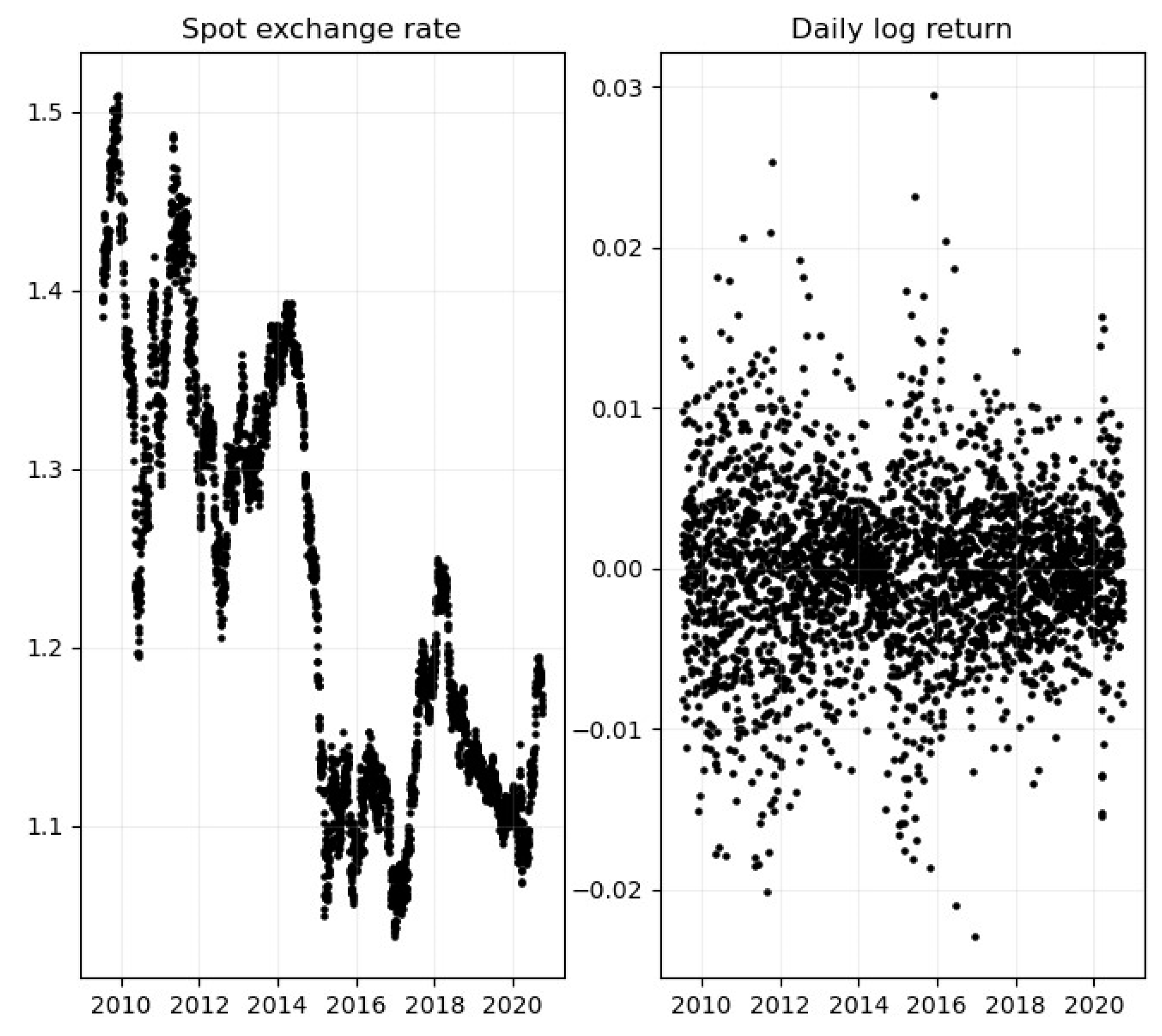
Figure 2.
Time series and empirical distributions for implied moments of 1–week to expiry options; at-the-money volatilities [panels (a) and (b)] and 25 delta risk reversals [panels (c) and (d)]. Time period; 2009:01-2020:09. Source; Bloomberg.
Figure 2.
Time series and empirical distributions for implied moments of 1–week to expiry options; at-the-money volatilities [panels (a) and (b)] and 25 delta risk reversals [panels (c) and (d)]. Time period; 2009:01-2020:09. Source; Bloomberg.
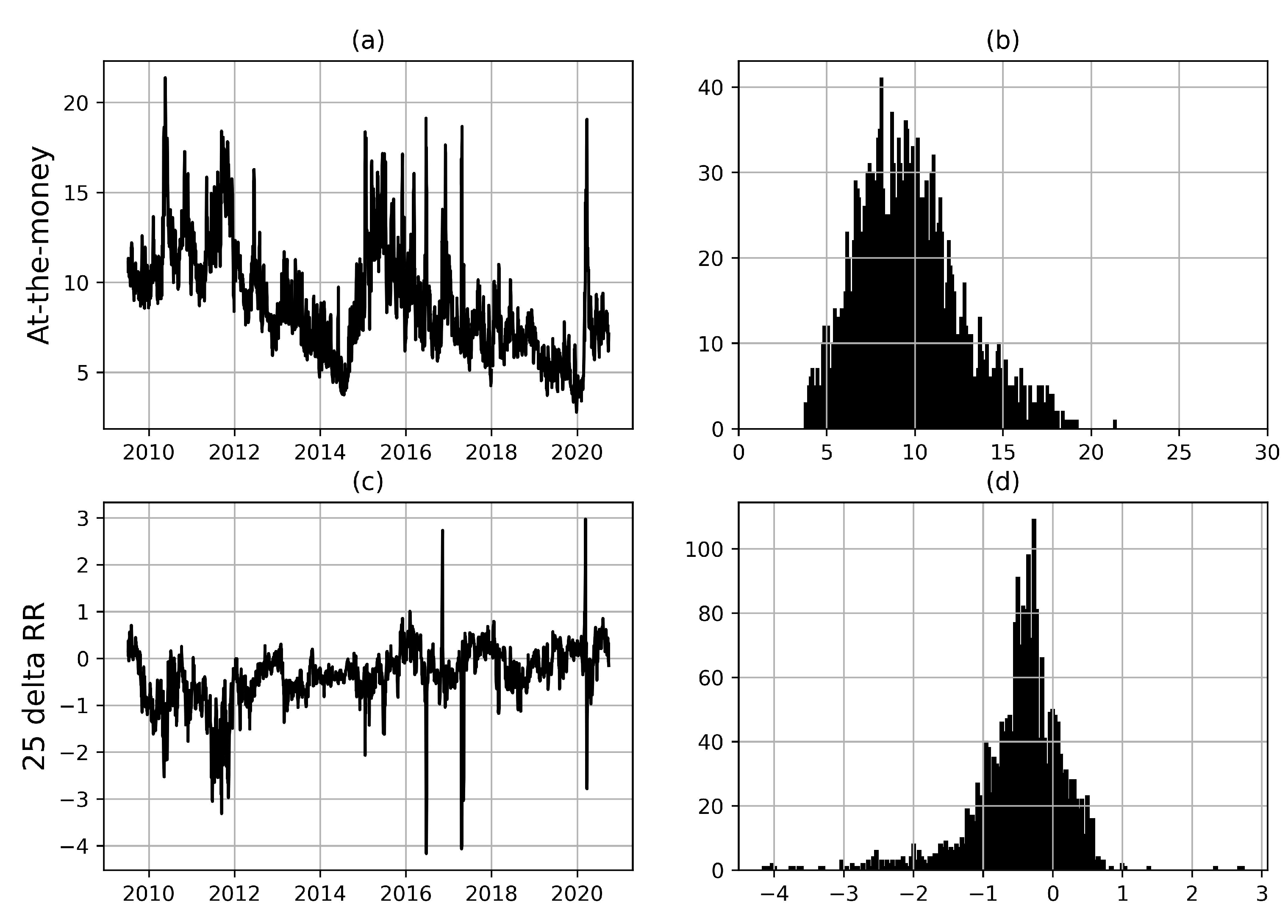
Figure 3.
Activation functions.
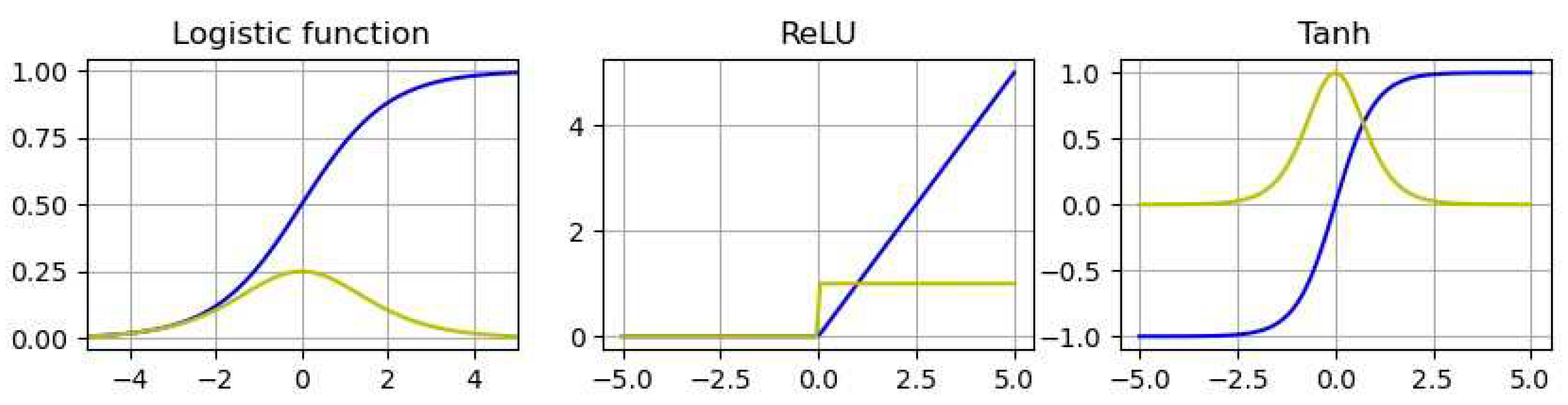
Figure 9.
Ensemble training period and validation period.
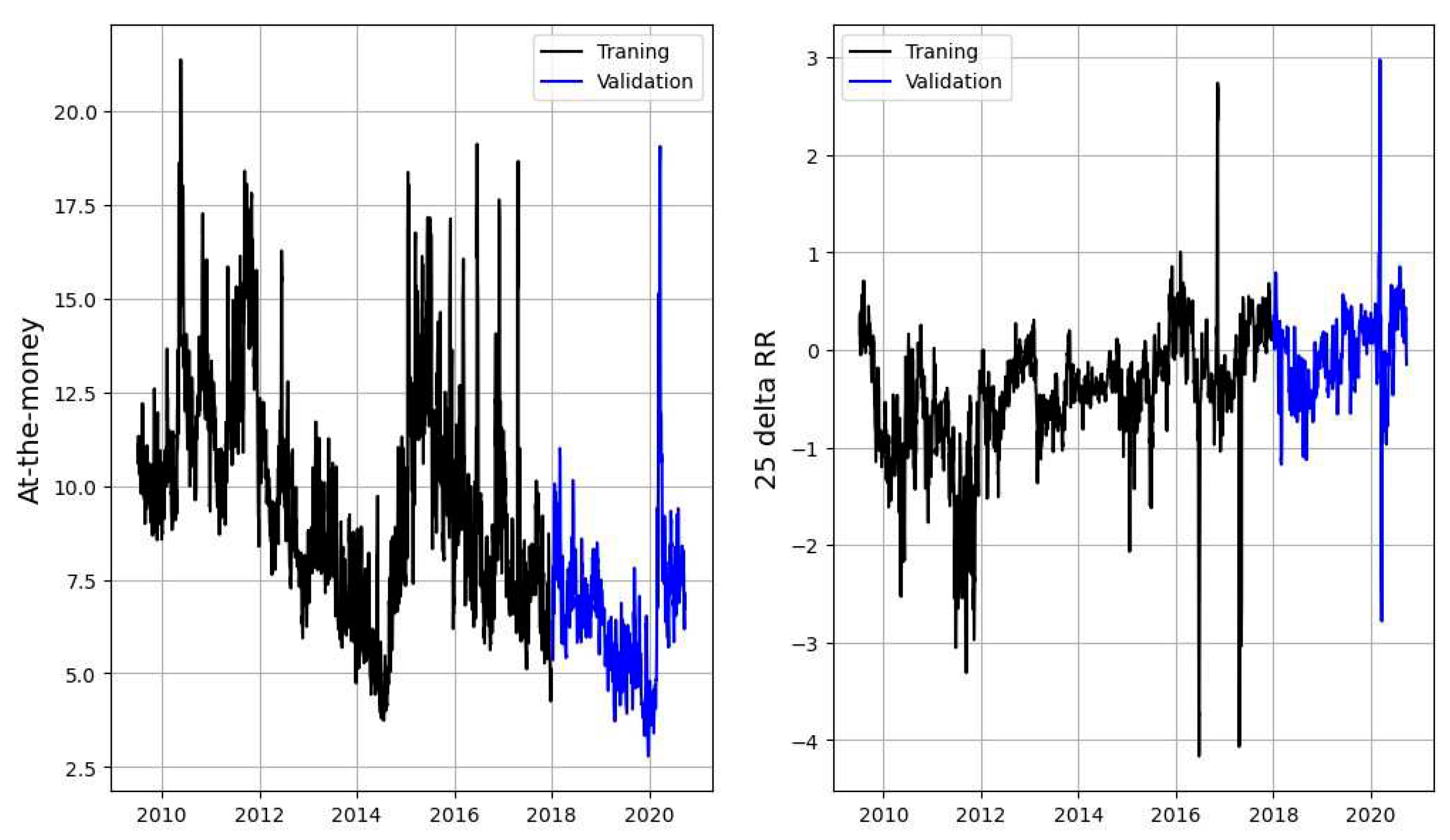
Figure 10.
Random Forest model. The black series is the daily log returns.
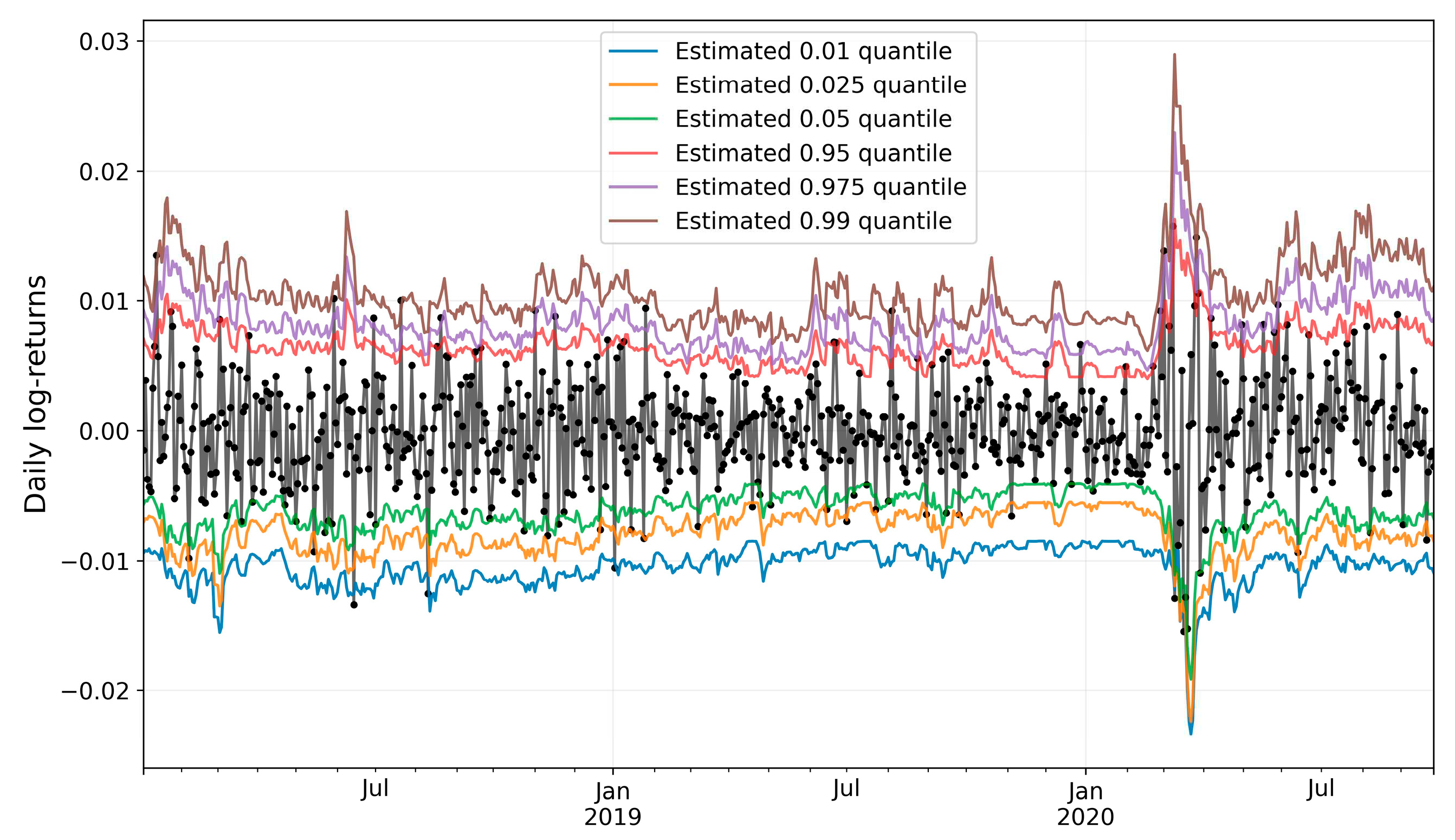
Figure 11.
Random Forest variable importance.
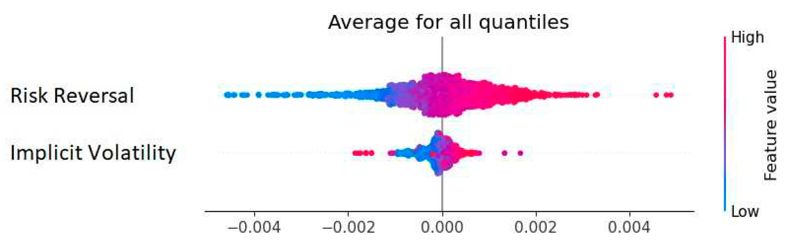
Figure 12.
Neural network training period and validation period.
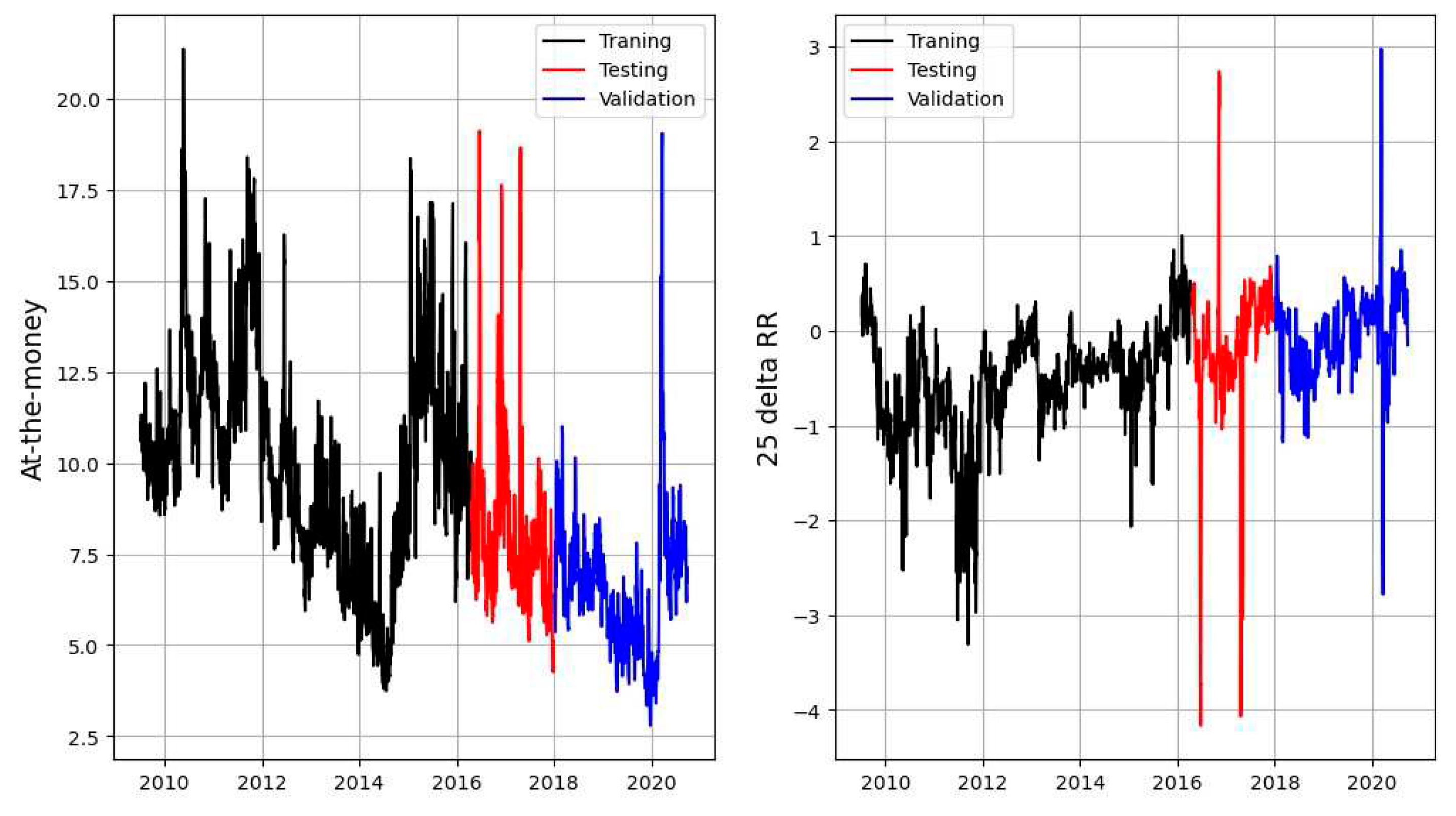

Table 1.
Descriptive statistics for daily EURUSD log-returns. Time period; 2009:01-2020:09. Source; Bloomberg.
Table 1.
Descriptive statistics for daily EURUSD log-returns. Time period; 2009:01-2020:09. Source; Bloomberg.
| n | 2930 |
| Mean | -0.0001 |
| Std. dev | 0.0053 |
| Skewness | 0.0330 |
| Kurtosis | 4.7508 |
| Min | -0.0229 |
| Max | 0.0295 |
Table 2.
QR-IM: ATM volatility, 25 delta risk reversal coefficients, along with the hit-percentage.
| Quantile – α | 1.0 % | 2.5 % | 5.0 % | 95.0 % | 97.5 % | 99.0 % |
| Constant | -0.61 (i) | -0.21 | -0.07 | 0.09 | 0.05 | 0.12 |
| ATM | -0.06 (i) | -0.09 (i) | -0.08 (i) | 0.09 (i) | 0.12 (i) | 0.15 (i) |
| 25-delta RR | 0.21 (i) | 0.16 (i) | 0.10 (ii) | 0.16 (i) | 0.30 (i) | 0.38 (i) |
| Breach Ratio | 1.04 | 2.48 | 4.97 | 94.99 | 97.43 | 99.01 |
Table 3.
Random Forest performance.
| Quantile – α | 1.0 % | 2.5 % | 5.0 % | 95.0 % | 97.5 % | 99.0 % |
| Breach Ratio | 0.7 | 2.1 | 5.75 | 95.09 | 97.62 | 99.44 |
| Sum if breach | -0.005 | -0.018 | -0.054 | 0.067 | 0.022 | 0.005 |
| Sum if no breach | -7.421 | -5.641 | -4.483 | 4.729 | 5.982 | 7.650 |
| Min. Var | -0.023 | -0.022 | -0.019 | 0.004 | 0.005 | 0.006 |
| Max. VaR | -0.008 | -0.005 | -0.004 | 0.016 | 0.023 | 0.029 |
Table 4.
The different data sets used for training the models. (*) A new movement variable was constructed, which captures the interaction between the ATM-variable and the RR-variable.
Table 4.
The different data sets used for training the models. (*) A new movement variable was constructed, which captures the interaction between the ATM-variable and the RR-variable.
| Model | Data set used for training |
| XGBoost (1) | QR-IM generated data set |
| XGBoost (2) | Gradient boost generated data set |
| LGBM (1) | QR-IM generated data set |
| LGBM (2) | QR-IM generated data set with new movement variable (*) |
| LGBM (3) | LGBM generated data set |
| Categorical Boosting | QR-IM generated data set |
| FFNN | QR-IM generated data set with new movement variable (*) |
| RNN | QR-IM generated data set with new movement variable (*) |
| LTSM | QR-IM generated data set with new movement variable (*) |
Table 5.
Summary of all model breach ratios.
| quantile – α | 1.0 % | 2.5 % | 5.0 % 95.0 % | 97.5 % | 99.0 % | |
| Base line model | -Breach Ratio- | |||||
| QR-IM Ensemble methods |
0.7 | 2.1 | 6.3 | 95 | 97.5 | 99.3 |
| Random Forest | 0.7 | 2.1 | 5.75 | 95.09 | 97.62 | 99.44 |
| XGB (1) | 0.7 | 2.1 | 5.47 | 95.09 | 97.9 | 99.44 |
| XGB (2) | 1.26 | 3.65 | 7.01 | 95.37 | 98.46 | 99.16 |
| LightGBM (1) | 0.55 | 1.82 | 5.33 | 95.09 | 97.62 | 99.44 |
| LightGBM (2) | 0.7 | 2.1 | 5.05 | 95.23 | 97.76 | 99.44 |
| LightGBM (3) | 1.4 | 4.49 | 8.42 | 95.65 | 96.63 | 99.3 |
| CatBoostStacking Models | 0.7 | 2.23 | 5.47 | 94.95 | 97.62 | 99.44 |
| LGBM2&CatBoostNeural network | 0.7 | 2.18 | 5.31 | 95.05 | 97.67 | 99.44 |
| FFNN | 2.38 | 4.35 | 8.27 | 90.74 | 96.21 | 98.74 |
| RNN | 2.42 | 4.27 | 7.68 | 90.75 | 96.02 | 98.72 |
| LTSM | 3.13 | 4.97 | 8.68 | 96.16 | 96.16 | 98.44 |
Table 6.
Summary of all model if breach values, i.b. and the if not breach values, i.n.b.
| quantile - α | 1.0 % | 2.5 % | 5.0 % | 95.0 % | 97.5 % | 99.0 % | |Sum| | |
| Ensemble methods | ||||||||
| Random Forest | i.b. i.n.b |
-0.005 -7.421 |
-0.018 -5.641 |
-0.054 -4.483 | 0.067 4.729 |
0.022 5.982 |
0.005 7.650 |
0.171 35.91 |
| XGB (1) | i.b. i.n.b. |
-0.006 -7.442 |
-0.019 -5.680 |
-0.052 -4.521 |
0.064 4.756 |
0.023 6.028 |
0.005 7.643 |
0.169 36.07 |
| XGB (2) | i.b. i.n.b. |
-0.025 -5.860 |
-0.056 -5.152 |
-0.184 -3.612 |
0.112 4.155 |
0.040 5.477 |
0.020 6.391 |
0.437 30.65 |
| LightGBM (1) | i.b. i.n.b. |
-0.004 -7.445 |
-0.017 -5.668 |
-0.053 -4.500 |
0.066 4.748 |
0.022 6.005 |
0.004 7.691 |
0.166 36.06 |
| LightGBM (2) | i.b. i.n.b. |
-0.005 -7.445 |
-0.019 -5.682 |
-0.055 -4.526 |
0.060 4.816 |
0.020 6.046 |
0.005 7.712 |
0.164 36.23 |
| LightGBM (3) | i.b. i.n.b. |
-0.020 -6.255 |
-0.054 -4.860 |
-0.104 -4.110 |
0.067 4.929 |
0.033 5.657 |
0.010 7.164 |
0.288 32.97 |
| CatBoost Neural network |
i.b. i.n.b. |
-0.006 -7.411 |
-0.020 -5.641 |
-0.056 -4.496 |
0.064 4.789 |
0.022 6.017 |
0.005 7.688 |
0.173 36.04 |
| FFNN i.b.i.n.b. | -0.052 -9.477 |
-0.098 -8.139 |
-0.188 -6.752 |
0.186 6.420 |
0.086 7.917 |
0.038 9.873 |
0.648 48.57 |
|
| RNN i.b.i.n.b. | -0.069 -9.120 |
-0.157 -8.486 |
-0.208 -6.287 |
0.201 6.274 |
0.088 8.406 |
0.047 10.064 |
0.770 47.00 |
|
| LTSM i.b.i.n.b. | -0.052 -9.303 |
-0.095 -8.114 |
-0.200 -6.529 |
0.213 6.132 |
0.110 7.346 |
0.046 9.242 |
0.716 46.66 |
|
Table 7.
Summary of all models containing p-values for the Christoffersen test and DQ-test (with four lags).
Table 7.
Summary of all models containing p-values for the Christoffersen test and DQ-test (with four lags).
|
Christoffersen test (p-value) |
1.0 % | 2.5 % | 5.0 % | 95.0 % | 97.5 % | 99.0 % |
| Random Forest | 0.398 | 0.489 | 0.364 | 0.364 | 0.846 | 0.200 |
| XGB (1) | 0.398 | 0.489 | 0.564 | 0.917 | 0.489 | 0.200 |
| XGB (2) | 0.175 | 0.000 | 0.000 | 0.000 | 0.157 | 0.001 |
| LightGBM (1) | 0.200 | 0.343 | 0.810 | 0.917 | 0.846 | 0.200 |
| LightGBM (2) | 0.398 | 0.489 | 0.945 | 0.781 | 0.660 | 0.200 |
| LightGBM (3) | 0.306 | 0.002 | 0.000 | 0.419 | 0.157 | 0.398 |
| CatBoost | 0.398 | 0.660 | 0.564 | 0.945 | 0.846 | 0.200 |
| DQ test (p-value) | 1.0 % | 2.5 % | 5.0 % | 95.0 % | 97.5 % | 99.0 % |
| Random Forest | 0.622 | 0.929 | 0.191 | 0.727 | 0.255 | 0.965 |
| XGB (1) | 0.806 | 0.944 | 0.192 | 0.280 | 0.858 | 0.965 |
| XGB (2) | 0.128 | 0.000 | 0.000 | 0.000 | 0.084 | 0.001 |
| LightGBM (1) | 0.673 | 0.938 | 0.319 | 0.648 | 0.717 | 0.964 |
| LightGBM (2) | 0.617 | 0.942 | 0.491 | 0.381 | 0.201 | 0.963 |
| LightGBM (3) | 0.000 | 0.001 | 0.000 | 0.951 | 0.506 | 0.991 |
| CatBoost | 0.692 | 0.943 | 0.371 | 0.678 | 0.204 | 0.964 |
Disclaimer/Publisher’s Note: The statements, opinions and data contained in all publications are solely those of the individual author(s) and contributor(s) and not of MDPI and/or the editor(s). MDPI and/or the editor(s) disclaim responsibility for any injury to people or property resulting from any ideas, methods, instructions or products referred to in the content. |
© 2023 by the authors. Licensee MDPI, Basel, Switzerland. This article is an open access article distributed under the terms and conditions of the Creative Commons Attribution (CC BY) license (http://creativecommons.org/licenses/by/4.0/).
Copyright: This open access article is published under a Creative Commons CC BY 4.0 license, which permit the free download, distribution, and reuse, provided that the author and preprint are cited in any reuse.


