

Submitted:
04 May 2023
Posted:
05 May 2023
You are already at the latest version
Abstract
In this article, we estimate the value of Government Expenditure on Education-GEE in the context of Environmental, Social and Governance-ESG dataset of the World Bank. We use data from 193 countries in the period 2011-2020. We use Panel Data with Fixed Effects, Panel Data with Random Effects, Pooled Ordinary Least Squares-OLS, and Weighted Least Squares-WLS. Our results show that the value of GEE is positively associated among others to “Case of Death, by communicable disease and maternal, prenatal and nutrition conditions”, and “Unemployment”, and negatively associated among others to “Hospital Beds” and “Government Effectiveness”. Furthermore, we apply the k-Means algorithm optimized with the Elbow Method and we find the presence of four clusters. Finally, we confront eight machine learning algorithms for the prediction of the future value of GEE. We found that the Polynomial Regression is the best predictive algorithm. The Polynomial Regression predicts an increase in GEE of 7.09% on average for the analysed countries.
Keywords:
Analysis of Collective Decision-Making
; General
; Political Processes: Rent-Seeking
; Lobbying
; Elections
; Legislatures
; Voting Behaviour
; Bureaucracy
; Administrative Processes in Public Organizations
; Corruption
; Positive Analysis of Policy Formulation
; Implementation
1. Introduction-Research Question
In the following article we take into consideration the role of GEE in the context of the ESG models. The originality of the article consists in considering the relationship between investment in the education and the application of ESG models. In fact, as indicated in the second paragraph, there are many scientific articles that have investigated the relationship between the managerial training to the ESG issues and the ESG performance of companies. In our case, on the contrary, we did not investigate the relationship between education and ESG model from a micro-economic or organizational point of view. Instead, we have analyzed the macro-economic dimension of the relationship between investment in GEE and the impact in terms of ESG. For this motivation we have analyzed a very large set of countries, i.e.193, using the ESG dataset of the World Bank. The role of education and managerial models in the management of public and private organizations is relevant. It is the managerial training that tends to determine the ability of companies to perform well or badly based on certain criteria, for example in their choice between profit maximization or stakeholder maximization [1,2,3,4]. The investigation of the role of education in necessary for a better comprehension of the impacts of ESG models at world level [5,6,7,8,9,10,11,12,13,14,15,16].
However, it is necessary to distinguish between developing and industrialized countries. In developing countries, education has both the function of the formation of human capital and the function of promoting economic development and avoiding poverty. In medium-high per capita income countries, on the other hand, education can be a lever to increase awareness and application of ESG models in companies. It is very probable that in the future the ESG model will be included in the MBA programs and engineering disciplines to raise consciousness regarding the issues of environmental, social, and ethical sustainability.
The article continues as follows: the second section contains a brief literature review, the third section discusses the econometric models, the fourth paragraph shows the results of the clustering with k-Means algorithm, the fifth paragraph contains the prediction with machine learning algorithms, the sixth paragraph concludes. The Appendix A contains further statistical results that have not found adequate space in the text.
2. Literature Review
A very short synthesis of literature is analyzed below concerning the relationship between ESG models and education levels. The literature on the topic is not clear, as there are not many articles that consider the impact of public spending on education in the percentage of the GDP on the ESG models. On the contrary, the value of education is considered not from a macro-economic point of view, as in the case of expenditure in the percentage of the GDP, but rather from the micro-economic point of view, or as the level of education of the managers and board members. A void is thus identified in the scientific literature that our article in part tends to fill.
CEO’s Education and ESG models. The role of the education of the CEOs to ESG methodologies is very relevant to allow the application of governance models that may be ESG compliant. Universities and companies should invest in the formation of new managerial training systems capable of orienting CEOs towards the application of ESG models. CEOs with degree in engineering, economics, and natural science show less sensitivity toward ESG performance in a set of 285 German companies listed in German DAX and MDAX [17]. Students that have attended to ESG courses during their MBA show greater sensitivity to work in companies with strong ESG commitment [18]. Directors that show greater interest in ESG values also produce deeper ESG disclosures in Islamic listed companies [19]. There is a positive relationship between Corporate Social Responsibility-CSR and business performance if CEOs are engineers of have an MBA degree [20]. The investment in ESG education is essential to promote ESG reporting at firm level [21].
Educational Issues and ESG policies. It is important to organize educational systems that are oriented towards the application of ESG models especially in economic and engineering disciplines. In fact, the lack of adequate training in terms of ESG reduces the ability of companies and markets to create products, services and methodologies that may be ESG compliant. Education is considered one of the essential issues for the evaluation of the ESG performance at corporate level [22]. Lack of adequate education is the main cause for the insufficient application of ESG models in Polish financial markets [23].
Female leadership and ESG models. One of the issues related to ESG models consists in the role of women within corporate governance systems. ESG models promote inclusion and gender equality. The expected effect is that the presence of a greater number of women within organizations can lead to a growth in the company's ability to have better performance in terms of ESG. There is no positive relationship between female leadership and the application of ESG models in China [24]. Female business leaders perform better in terms of ESG in a set of 2278 European companies, especially in contrasting unethical behavior [25]. There is a positive relationship between female leadership and ESG models in a set of 556 U.S. firms [26].
ESG models in higher education. The application of ESG models within university management is necessary to increase the orientation towards sustainability, inclusion, and the ethics of governance. Obviously, there are two methodologies to introduce ESG models within the functioning of university: the first consists in organizing a courses, degrees and masters centered on ESG models, the second consists in identifying a set of university management practices in the logic of ESG to allow the university workforce to generate results in terms of sustainability, inclusion, and ethics. An example of the application in the governance of university of ESG model consists in recognizing the value of gender parity and LGBT+ people in the faculty. The application of ESG models in higher education institutions can help universities to achieve the goals of Sustainable Development Goals-SDGs [27]. ESG models in higher education should apply ESG models and promote a DEI approach even among faculty members [28].
ESG critiques. One of the problems with ESG models concerns their ability to give a real representation of the performance of companies and organizations to invest in some valuable goods such as sustainability. ESG models tend to be excessively generic. The ESG indicators are in fact made up of a complex structure that brings together various elements and may be missing of the depth to analyze the individual aspects in the field of ESG structures. For example, ESG models are criticized for not having the ability to correctly quantify the various dimensions of environmental sustainability [29].
ESG scores and investments in education. Finally, we can observe that education is one of sectors in which ESG oriented found tends to invest. Private investors that follow the ESG approach tend to invest in ethical sector such as in education [30]. The interest of ESG based found for the education sector is due to the strategic role of universities and schools as a force to change mentality either in the professional sphere either in the general pop-culture.
3. The Econometric Model
An econometric analysis for estimating the determinants of the GEE value is presented below. The data analysed refer to 193 countries in the period between 2011 and 2020. The dataset used is the Environmental, Social and Governance-ESG of the World Bank. The data were analysed using the Panel Data with Fixed Effects, Panel Data with Random Effects, Pooled OLS and WLS. Specifically, we have estimated the following formula:
where and The value of GEE is positively associated to:
- CD: refers to the share of all deaths for all ages from underlying causes. Communicable diseases and maternal, prenatal, and nutritional conditions include infectious and parasitic diseases, respiratory infections, and nutritional deficiencies such as underweight and stunting. There is a positive relationship between the CD value and the GEE value. This relationship is because the countries that have higher levels in terms of GEE are also countries with low per capita income with high mortality. For example in the top five countries by value of GEE there are: Mongolia with 38.10%, Sierra Leone with 35.00%, Solomon Islands with 30.06%, Namibia with 26.39%, Uzbekistan with 25.59%. Conversely, countries that have a medium-high per capita income tend to spend smaller percentages of GDP for GEE as for example in the case of the United States with 13.38%, Australia with 12.48%, the Netherlands with 12.51%, Belgium with 12.23%, Germany with 11.37%. The greater investment of low per capital countries in GEE is since these countries need education either to escape from poverty either to promote the increase in the human capital of the population.
- UT: refers to the share of the labour force that is without work but available for and seeking employment. There is a negative relationship between the value of UT and the value of GEE. Countries that have higher value of GEE are countries with low per capita income with high levels of unemployment. In these countries, the investment in education also has the social function of fighting against poverty, deprivation, and the lack of human rights. Education for countries with low per capita income is in fact more a policy to promote economic development than a policy aimed at increasing the cultural level of the population. On the contrary, in countries with higher per capita income, such as Western countries, the GEE value tends to be lower in relation to a reduced UT value thanks to the greater and better employment opportunities offered by the labour market.
- TMPA: are totally or partially protected areas of at least 1,000 hectares that are designated by national authorities as scientific reserves with limited public access, national parks, natural monuments, nature reserves or wildlife sanctuaries, protected landscapes, and areas managed mainly for sustainable use. Marine protected areas are areas of intertidal or subtidal terrain--and overlapping water and associated flora and fauna and historical and cultural features--that have been reserved by law or other effective means to protect part or the entire enclosed environment. Sites protected under local or provincial law are excluded. There is a positive relationship between TMPA and GEE. This relationship is because countries with high levels of GEE, which are often countries with low per capita income, also have vast natural resources including protected areas.
- FPI: covers food crops that are considered edible and that contain nutrients. Coffee and tea are excluded because, although edible, they have no nutritional value. There is a positive relationship between FPI and GEE. This relationship is because countries that have high levels of GEE are also countries with significant agricultural production. In fact, it is typical of countries with low per capita incomes to have a high agricultural component of GDP. In fact, these countries also tend to export their crops. Conversely, countries that have a medium-low GEE value, including Western countries, have a very negligible agricultural component in their GDP, as their economies generate wealth through the service and high-tech sectors.
- EU: refers to use of primary energy before transformation to other end-use fuels, which is equal to indigenous production plus imports and stock changes, minus exports and fuels supplied to ships and aircraft engaged in international transport. There is a positive relationship between EU and GEE even if the coefficient in the regression analysis is close to zero. The reason for a positive trend between these two variables is that countries that have high levels of GEE are also countries with low per capita income. Countries with low per capita income tend to have higher Gross Domestic Product growth rates. The augment of the GDP is also possible thanks to an increase in energy consumption. This results in a positive relationship between the EU and the GEE. In countries with higher per capita incomes, there is not only a lower level of GEE, but there is also greater attention to energy efficiency as indicated in the hypothesis of the Environmental Kuznets Curve-EKC.
| Estimations of the GEE | |||||||||
| Variables | WLS | Pooled OLS | Fixed Effects | Random Effects | Average | ||||
| Coefficient | P-Value | Costant | P-Value | Costant | P-Value | Costant | P-Value | ||
| Costant | 24,095 | *** | 35,915 | *** | 157,607 | ** | 22,988 | *** | 246,896 |
| GE | -0,4529 | *** | -0,47001 | ** | -0,14383 | *** | -11,459 | *** | -0,55314 |
| CD | 0,1860 | *** | 0,18895 | *** | 0,11273 | *** | 0,1181 | *** | 0,15146 |
| EU | 0,0003 | *** | 0,00027 | *** | 0,00043 | *** | 0,0004 | *** | 0,00036 |
| FPI | 0,0748 | *** | 0,05765 | *** | 0,03029 | *** | 0,0354 | *** | 0,04954 |
| HB | -0,4008 | *** | -0,52122 | *** | 0,36931 | *** | 0,1951 | * | -0,0894 |
| TMPA | 0,0803 | *** | 0,11136 | *** | 0,13667 | *** | 0,1296 | *** | 0,11448 |
| UT | 0,0576 | ** | 0,09108 | ** | 0,25656 | *** | 0,17 | ** | 0,14379 |
The value of GEE is negatively associated to:
- HB: include inpatient beds available in public, private, general, and specialized hospitals and rehabilitation centres. In most cases, beds for both acute and chronic care are included. There is a negative relationship between HB and GEE. Countries that have high levels of GEE, i.e. countries that have low levels of per capita income, also have low levels of HB. In fact, countries with low per capita income lack the resources to implement an efficient health system. The HB number therefore tends to decrease in these countries. Conversely, in countries with high per capita income there is a greater availability of HB and a lower value of GEE. In fact, in countries with high per capita income, the aging of the population tends to increase health care expenditure with positive effects in terms of HB.
- GE: captures perceptions of the quality of public services, the quality of the civil service and the degree of its independence from political pressures, the quality of policy formulation and implementation, and the credibility of the government's commitment to such policies. Estimate gives the country's score on the aggregate indicator, in units of a standard normal distribution, i.e. ranging from approximately -2.5 to 2.5. There is a negative relationship between the value of GEE and the value of GE. In fact, the countries that have high levels of GEE are countries with low per capita incomes and with political and democratic institutions lacking the necessary credibility to guarantee a high level of GE. Conversely, Western countries where there is a high GE value have low GEE levels. However, in the long run, the investment in GEE should also increase the value of GE in low per capita income countries.
4. Clusterization with k-Means Algorithm Optimized with the Elbow Method
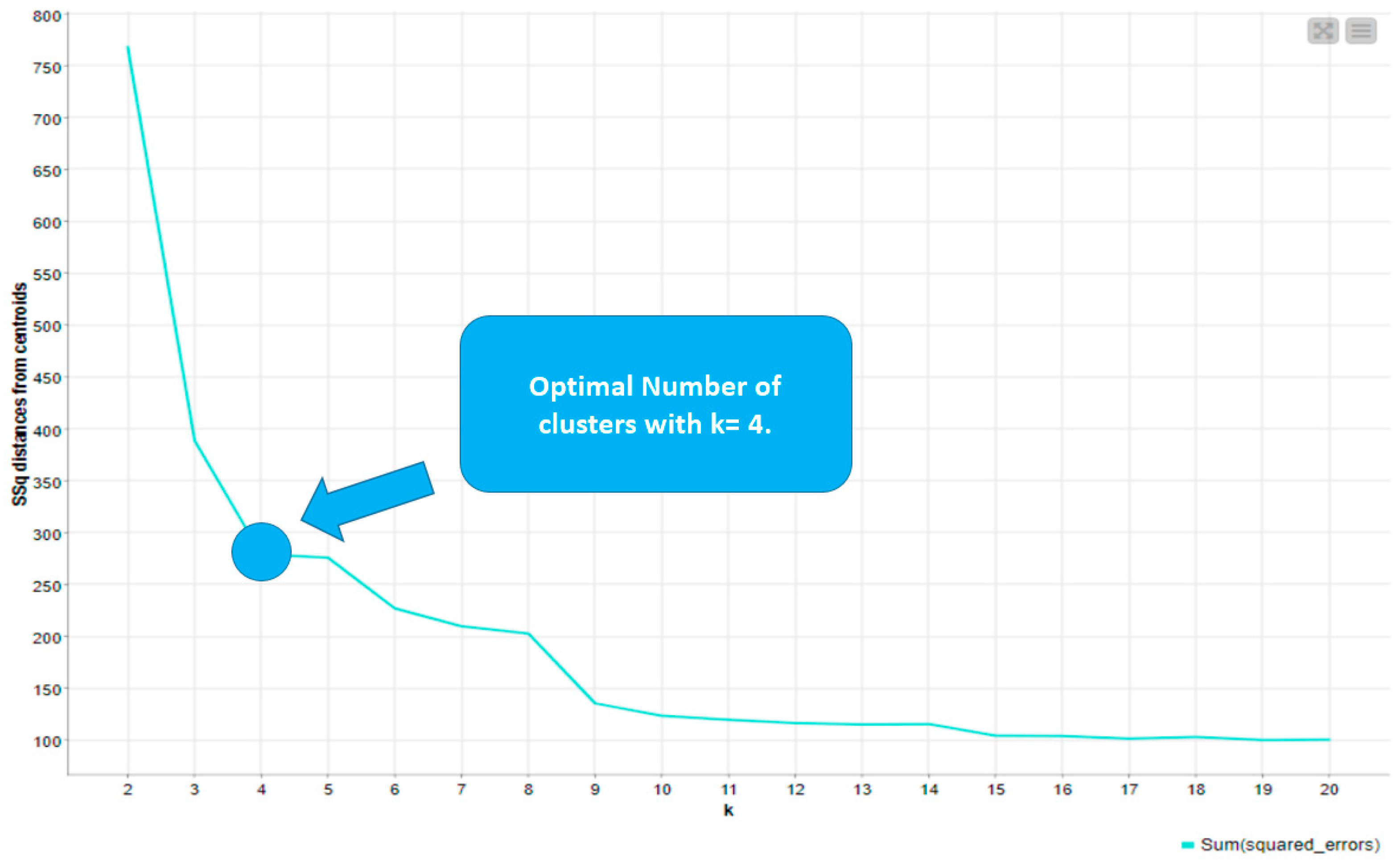
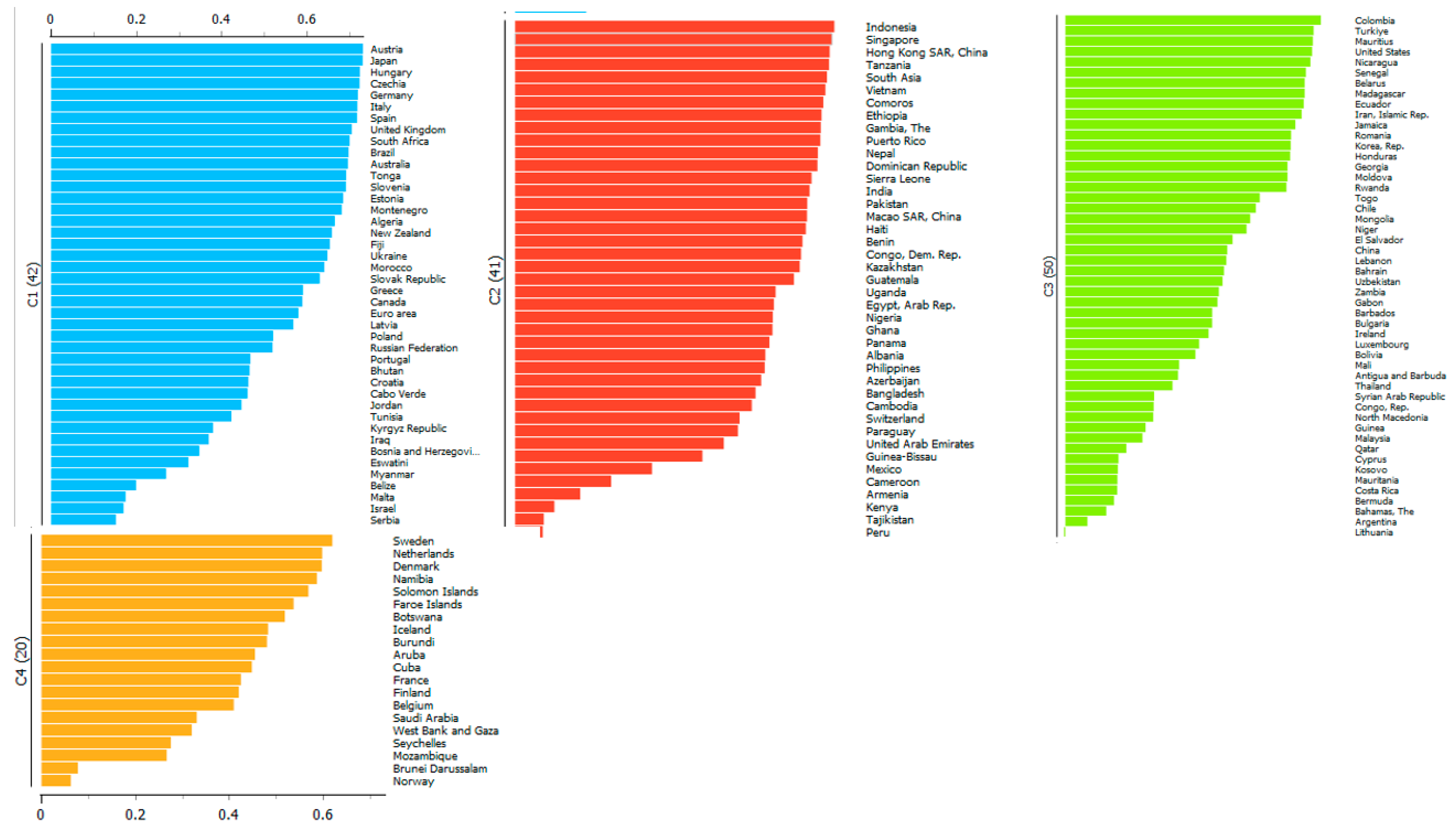
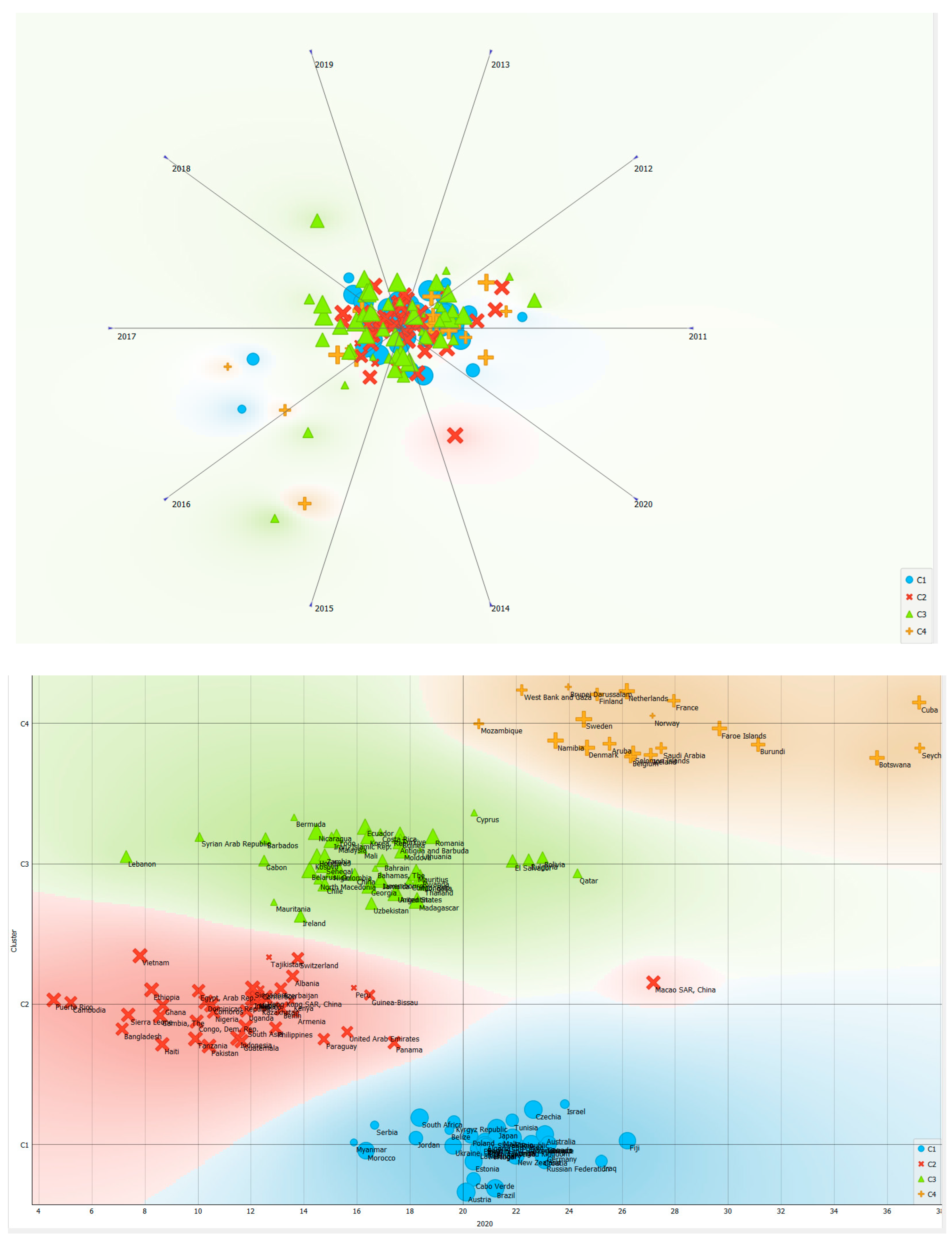
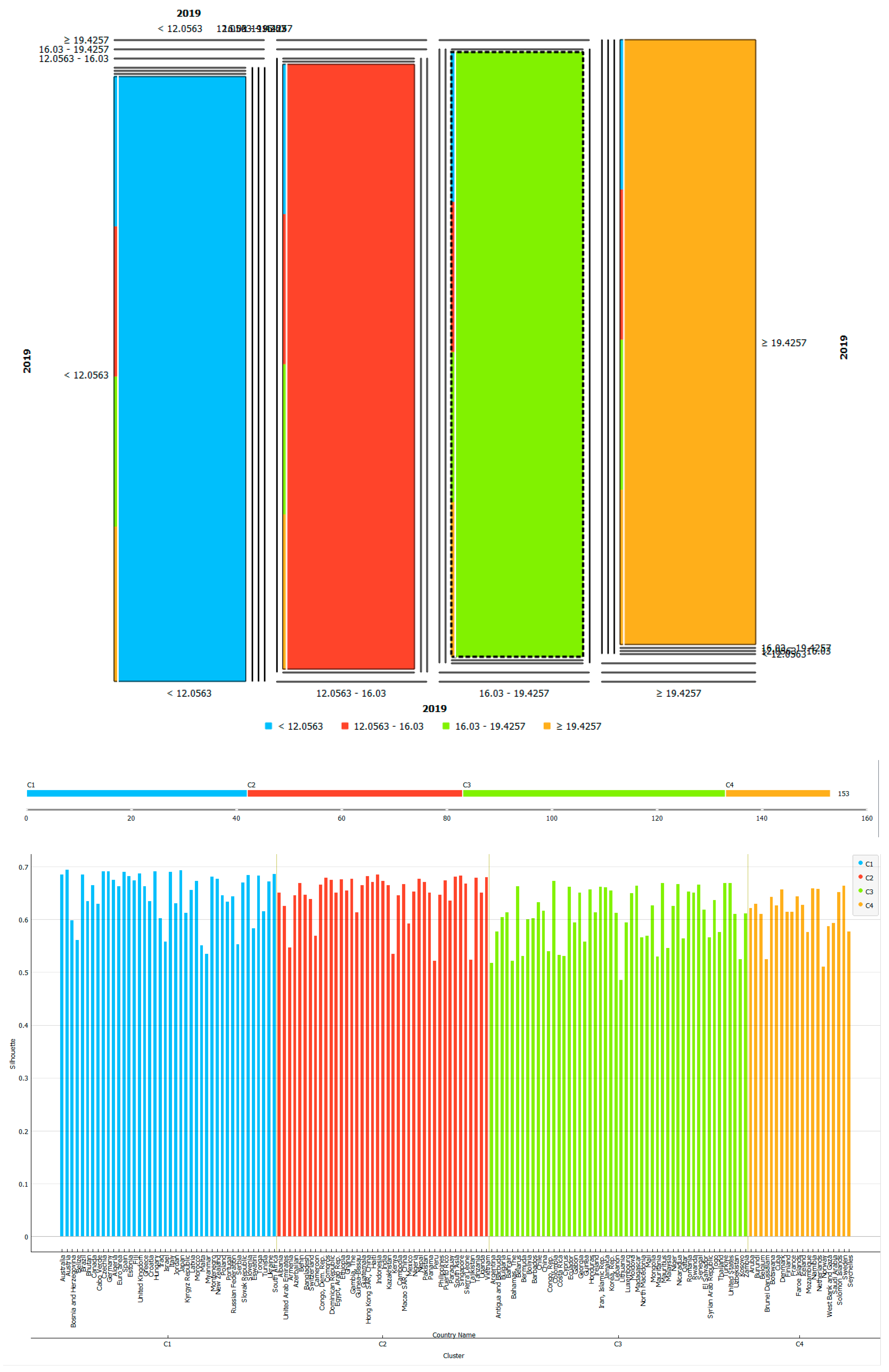
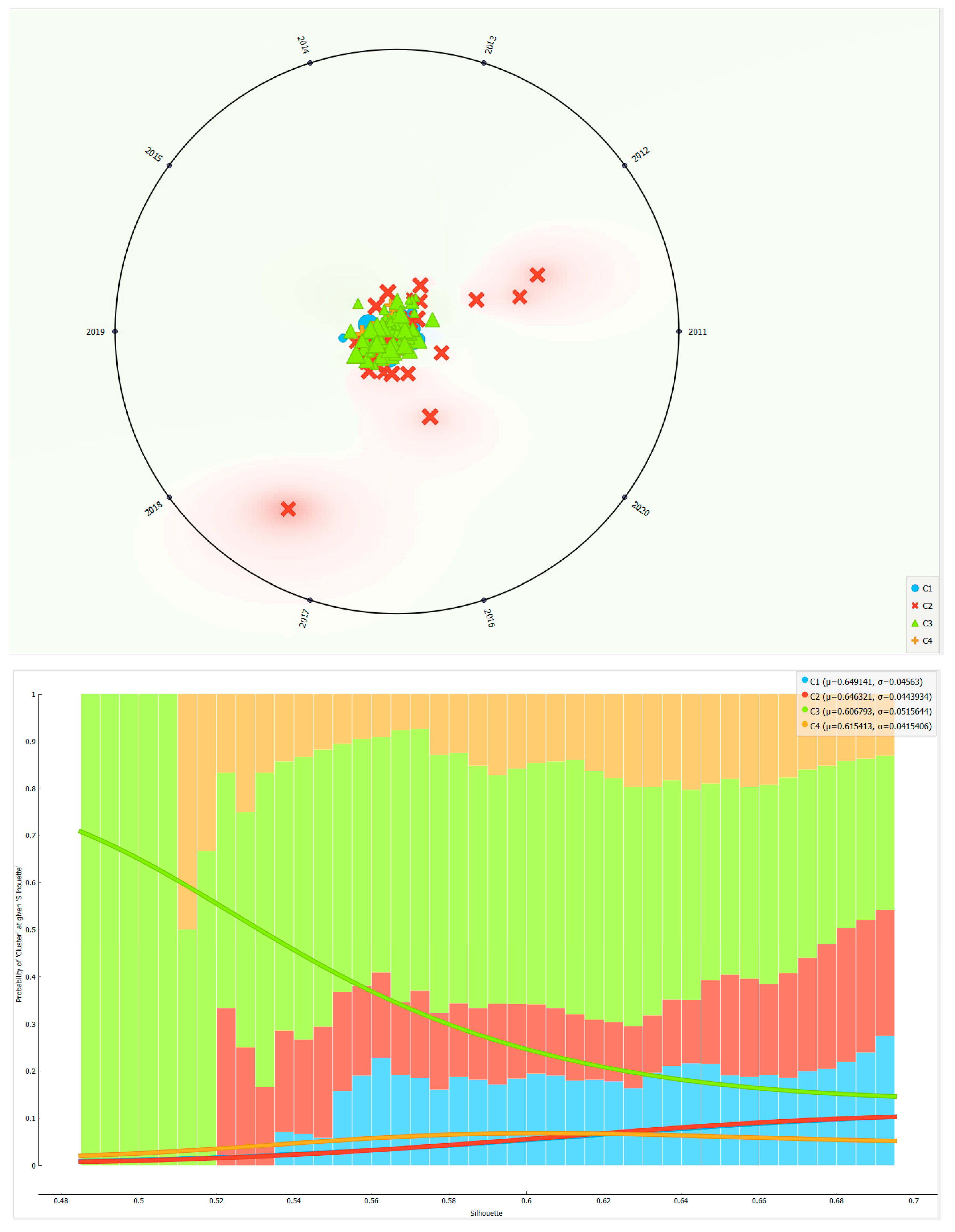
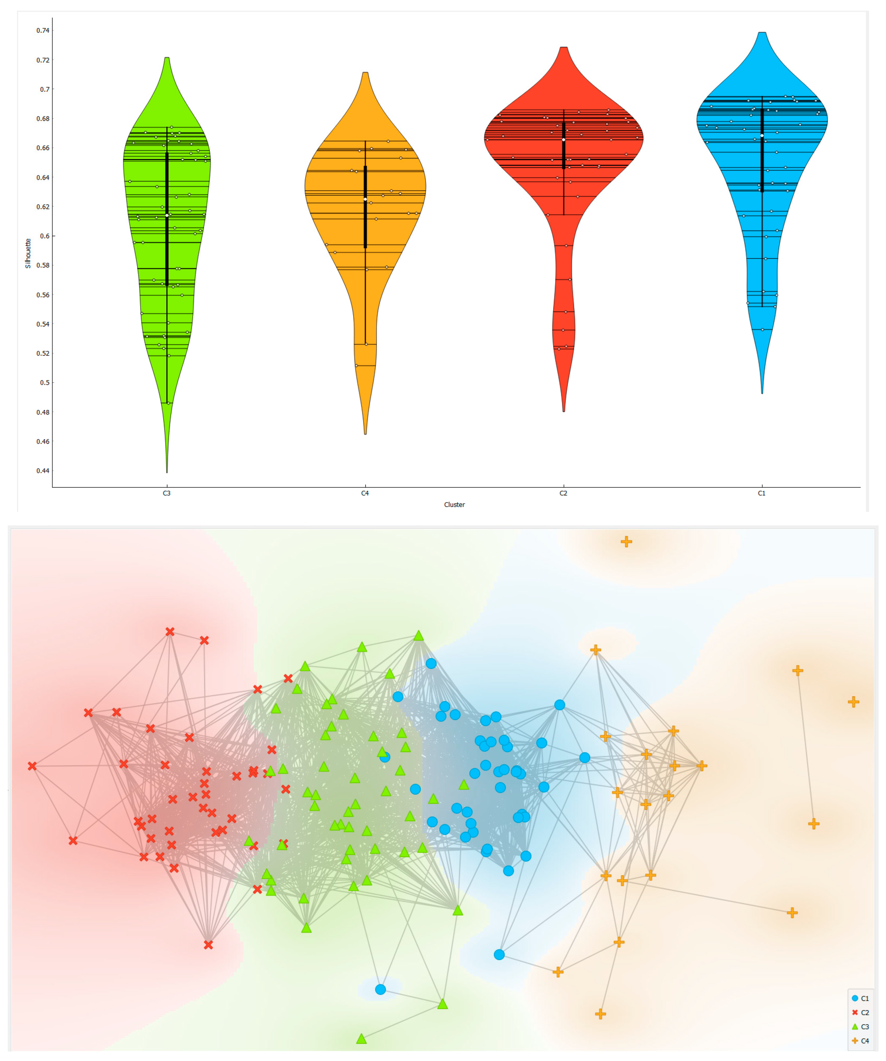
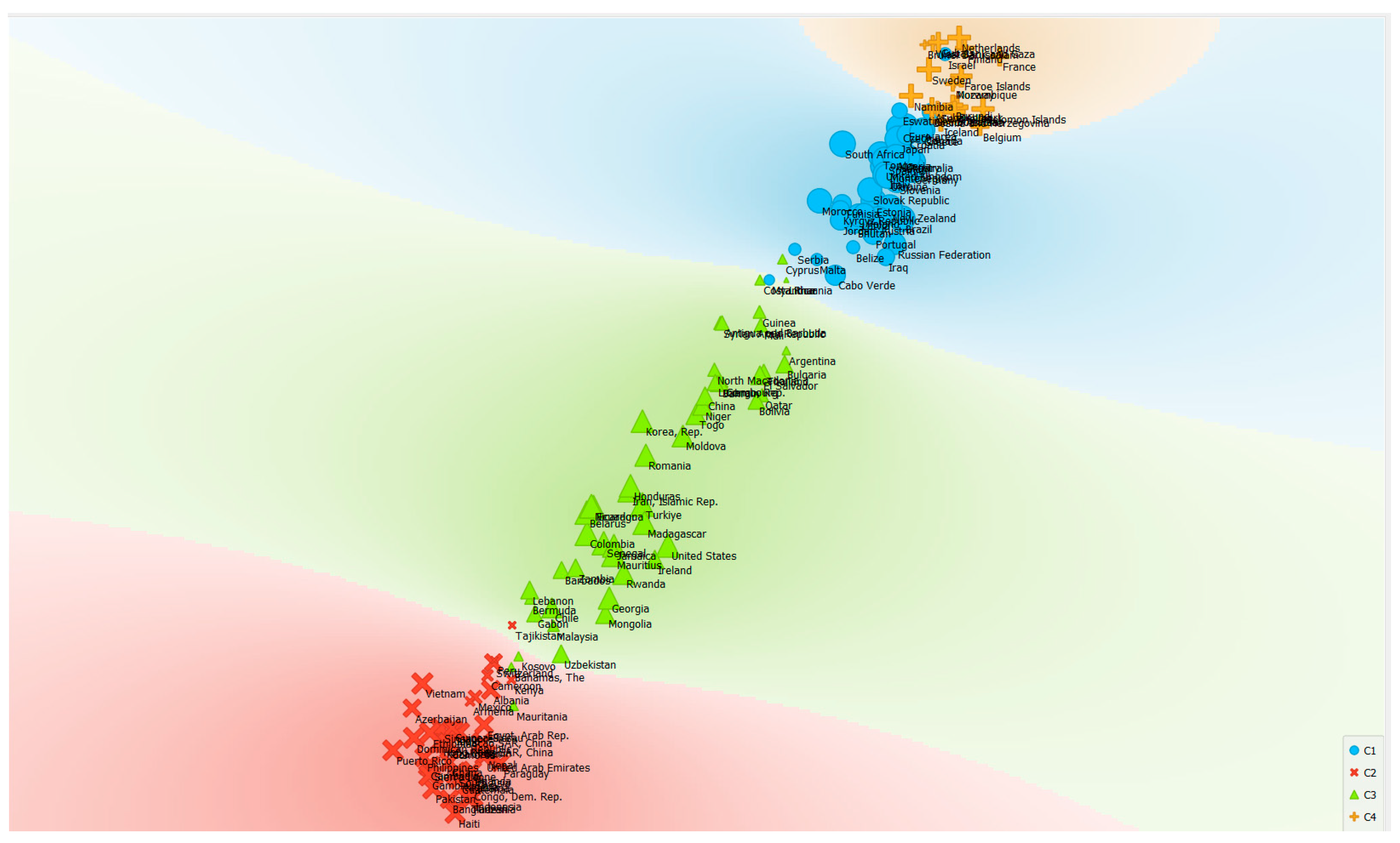
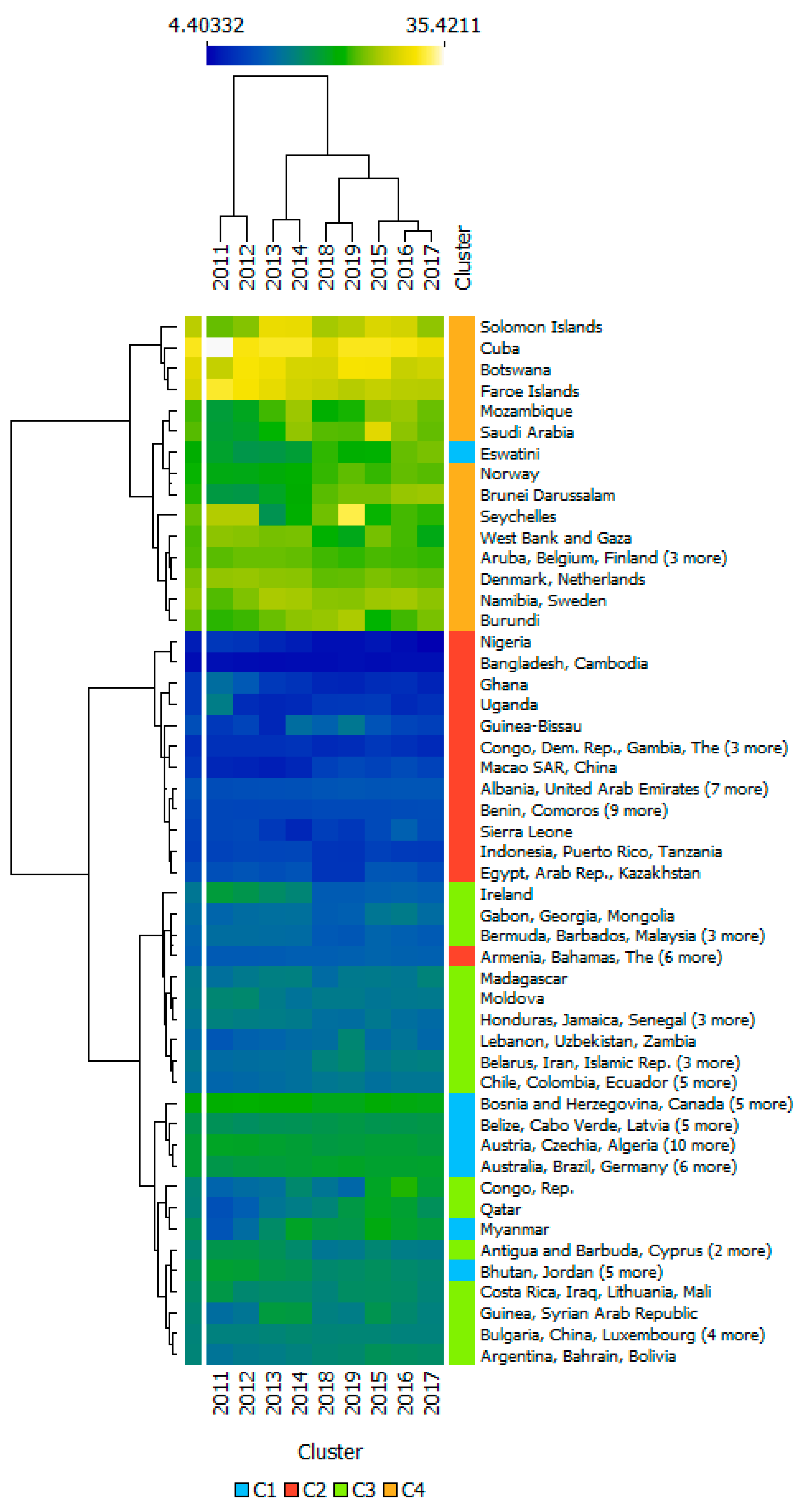
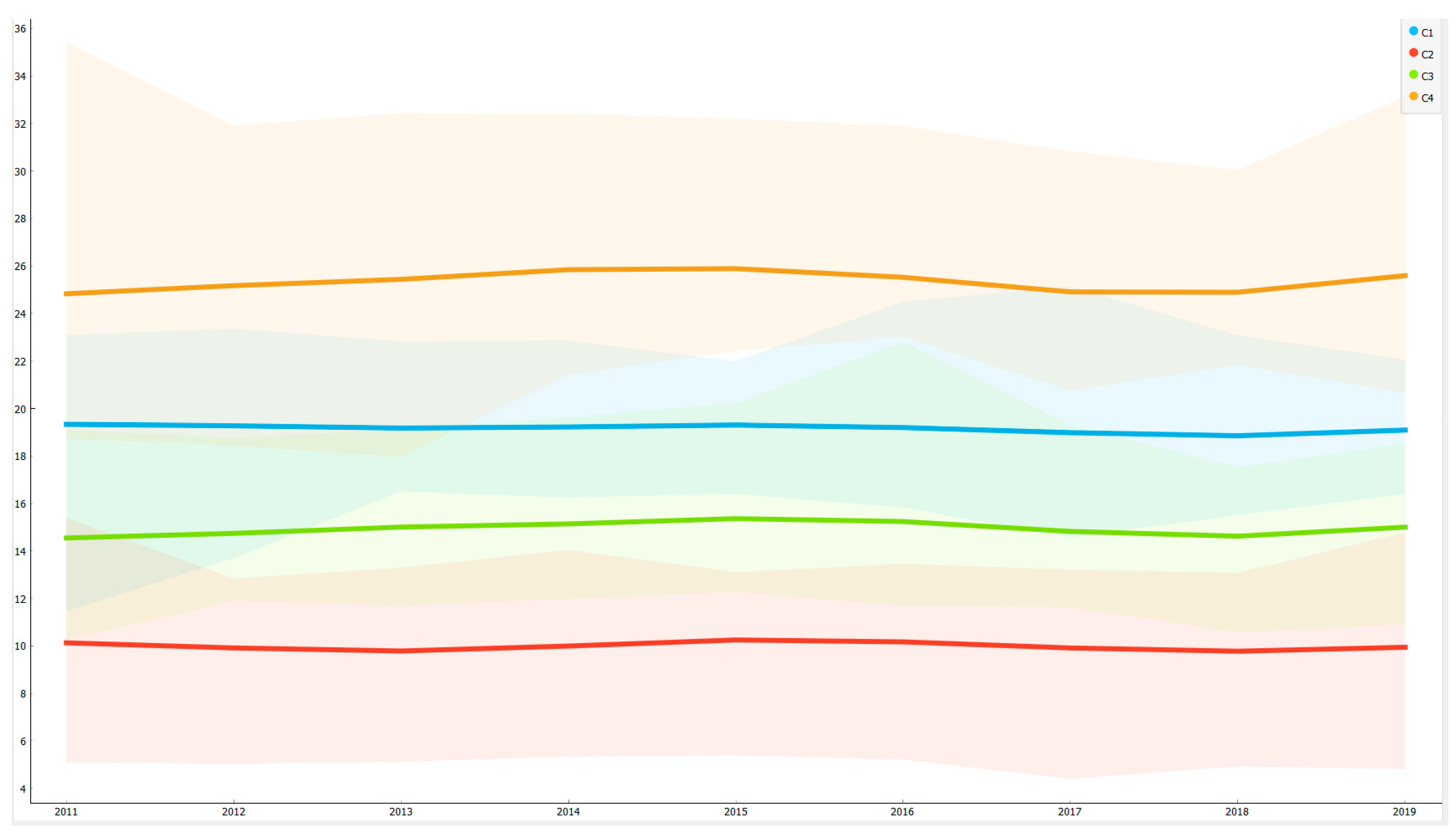
In the following analysis, we consider a clustering with k-Means algorithm. Since the k-Means algorithm is unsupervised, it follows that it is necessary to indicate the optimal number of k, i.e. clusters. We use the Elbow method to identify the optimal number of clusters. We have found four clusters using the Elbow method. The ranking of the clusters in terms of GEE is indicated below: C4>C1>C3>C2.
Figure 1.
Optimal Number of Clusters with k=4.
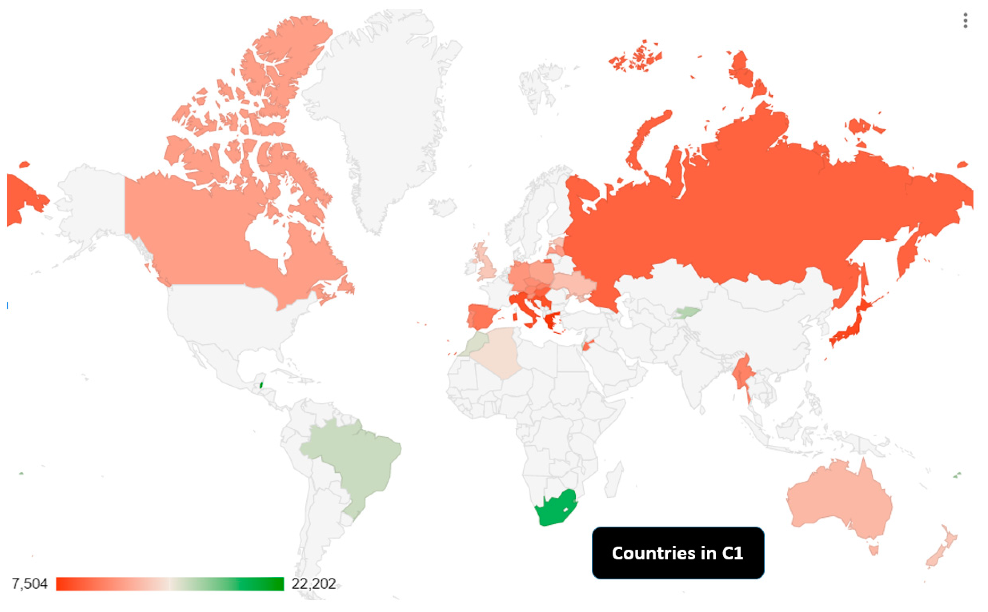
- Cluster 1: Austria, Japan, Hungary, Czechia, Germany, Italy, Spain, United Kingdom, South Africa, Brazil, Australia, Tonga, Slovenia, Estonia, Montenegro, Algeria, New Zealand, Fiji, Ukraine, Morocco, Slovak Republic, Greece, Canada, Latvia, Poland, Russian Federation, Portugal, Bhutan, Croatia, Cabo Verde, Jordan, Tunisia, Kyrgyz Republic, Iraq, Bosnia and Herzegovina, Eswatini, Myanmar, Belize, Malta, Israel, Serbia. C1 is the second cluster in terms of GEE. Brazil, South Africa, Morocco and the Kyrgiz Republic are the countries that invest most in education as percentage of GDP. The value of GEE in these countries is high for at least two reasons: first, these countries invest in education to participate in the knowledge economy and optimize their value added in the digital economy; second, these countries have low per capita income. In effect, countries with low per capita income tend to have a higher GEE. In fact, if we look within C1 countries, we see that countries with a higher per capita income have lower GEE then countries with lower per capita income. However, there are exceptions i.e. Ukraine, Vietnam and Jordan that, despite having low average values of per capita income have low levels of GEE, among C1 countries. However, the trend that we can gather from the analysis of C1 is that the value of the investment in GEE is inversely proportional to the value of per capita income. Finally, some considerations are necessary for Russia. Russia is a controversial country from an economic point of view. In fact, if, on the one hand Russia can be considered as a developing country in terms of GDP per capita, on the other hand, it is necessary to consider Russia as a global player due to military force and natural resources. Furthermore, the role of Russia seems improved within the groups of BRICS countries and their intention to create a unique currency alternative to the U.S. dollar [31]. However if we look at life expectancy in Russia, we can see that it is low either in respect to Eastern Europe countries, suggesting that an increase in the GEE and healthcare expenditure could be strongly recommended.
Figure 2.
Countries in C1.
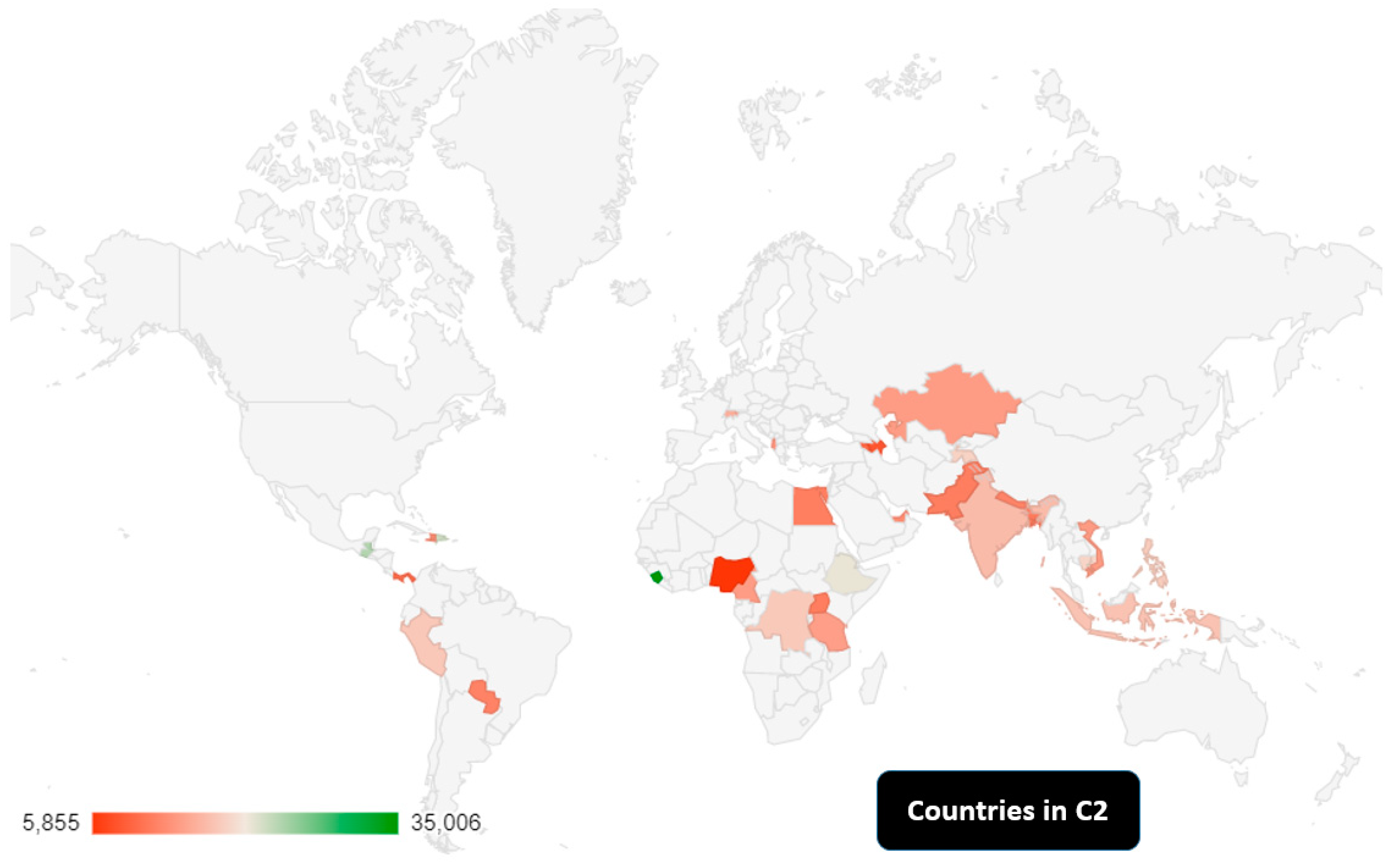
- Cluster 2: Indonesia, Singapore, Hong Kong, Tanzania, Vietnam, Comors, Ethiopia, The Gambia, Puerto Rico, Nepal, Dominica Republic, Sierra Leone, India, Pakistan, Macao SAR, Haiti, Benin, Congo Dem. Rep., Kazakhstan, Guatemala, Uganda, Egypt Arab Rep., Nigeria, Ghana, Panama, Albania, Philippines, Azerbaijan, Bangladesh, Cambodia, Switzerland, Paraguay, United Arab Emirates, Guinea-Bissau, Mexico, Cameroon, Armenia, Tajikistan, Peru. C2 is the last cluster in terms of GEE. It is a composite cluster in geographical terms even if from an economic point of view it is quite homogeneous being made up of countries that have low per capita income levels, with the exception of Switzerland, Singapore and the United Arab Emirates. Some of these countries will be the protagonists of the global economic scene of the future as for example in the case of India, Indonesia, Egypt, Bangladesh, and Nigeria. Other countries are growing fast in per capita income and tend to become high middle per capita income countries as for example in the case of Albania. Furthermore, there are countries in C2 that experience conditions of war or poverty due to conflicts such as, for example, in the case of Ethiopia and Uganda.
In the future development of C2 countries there will certainly be an increase in GEE for India, Indonesia, Nigeria, Egypt, and Bangladesh. In fact, for these countries, the growth in the value of investment in education is necessary to increase competitiveness within the knowledge economy. Finally, the trend of GEE in Ethiopia could be difficult to predict following the political condition of the country, which suffers for conflict and war. C2 countries, in order to have full access to the knowledge economy, digitization, the information revolution, will have to invest further in terms of GEE to allow the population to acquire the necessary skills to access new production methods and participate in economic growth.
Figure 3.
Countries in C2.
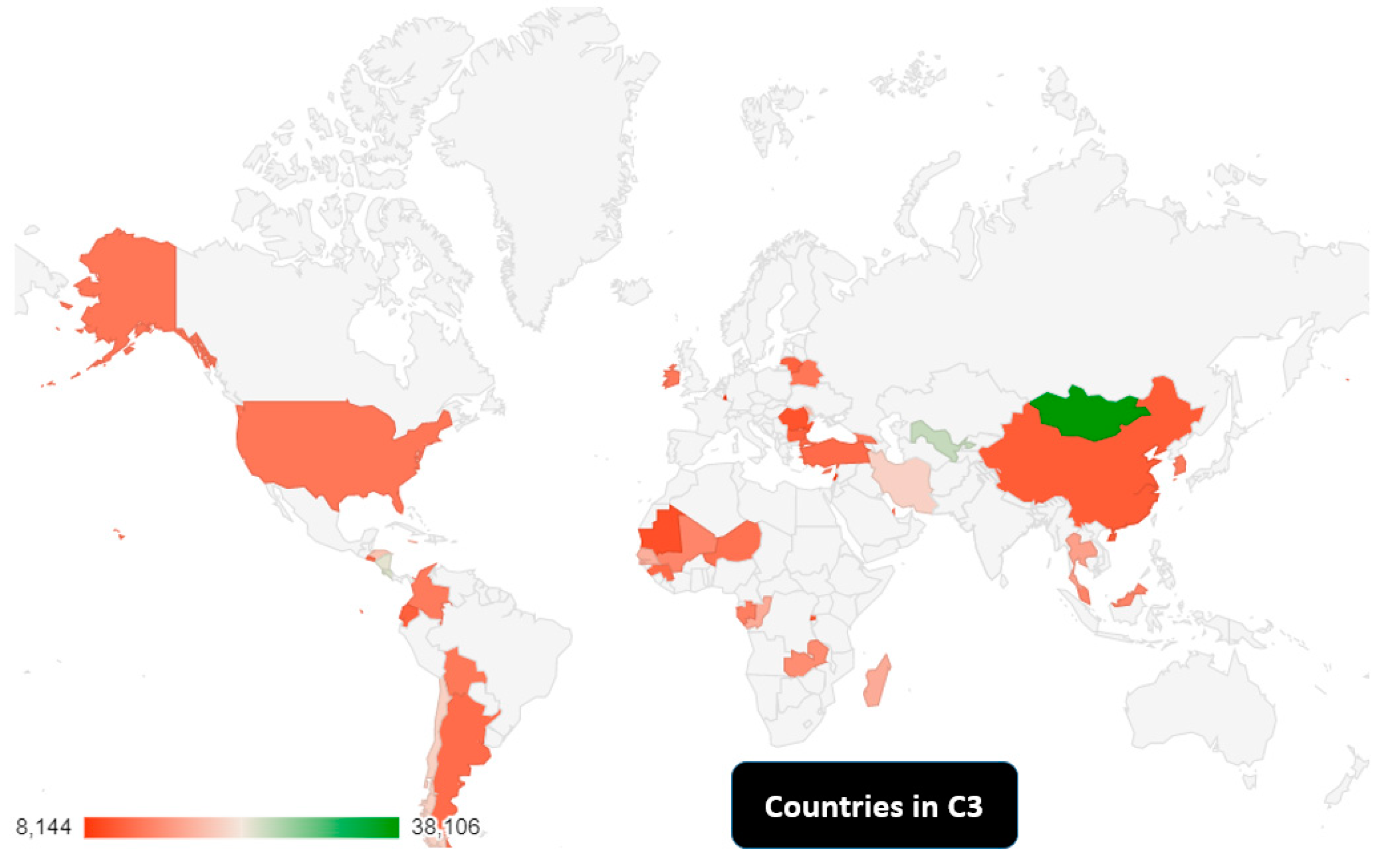
- Cluster 3: Colombia, Turchia, Mauritius, United States, Nicaragua, Senegal, Belarus, Madagascar, Ecuador, Iran, Jamaica, Romania, Korea Rep., Honduras, Georgia, Moldova, Rwanda, Togo, Chile, Mongolia, Niger, El Salvador, China, Lebanon, Bahrain, Uzbekistan, Zambia, Gabon, Barbados, Bulgaria, Ireland, Luxembourg, Bolivia, Mali, Antigua and Barbuda, Thailand, Syrian Arab Republic, Congo Rep., North Macedonia, Guinea, Malaysia, Qatar, Cyprus, Kosovo, Mauritania, Costa Rica, Bermuda, The Bahamas, Argentina, Lithuania. The C3 is in third place by value of GEE. It is a composite cluster both geographically, economically, and strategically. The C3 cluster includes a group of countries such as the USA, China, Turkey, and Ireland together with African and Latin American countries. Iran and Syria are also countries in C3. Their case is interesting since these countries suffer from embargo and war. However, even in these worse conditions, they are able to invest in terms of GEE and participating in the same cluster with U.S.A., Luxembourg, South Korea and Ireland. As a result, some countries, albeit in very different economic conditions and with various geographical locations, have similar levels of investment in GEE. If we consider the developing of GEE in the future, among C2 countries then we can observe that for sure the level of GEE in USA and European C2 countries will growth. The level of GEE will growth in USA according to the re-industrialization of the country and the intentions of the U.S. government to gain new competitiveness against the Chinese economy in terms of Research and Development, human capital, and the entire educational system. The investment in GEE is crucial in the tech-rivalry between US and China. For similar reasons, also the Chinese government will increase the expenditure in education as percentage of GDP due to the necessity to create new intangibles following the decision of the US government to reduce the technological transfers in the country. The technological competition between U.S. and China will increase the level of GEE in both countries. Similar results can be obtained in European countries. In effect, Italy and Spain are associated in the same cluster with Eastern countries even if there are significant difference between the two subgroups in terms of GDP per capita. Specifically, the level of GEE in Italy and Spain should converge with that of France and Scandinavian countries according to the suggestion of European Union that has incentivized EU members to improve the R&D/GDP ratio to 3%. Easter European countries will have similar paths of Italy and Spain.
Figure 4.
Countries in C3.
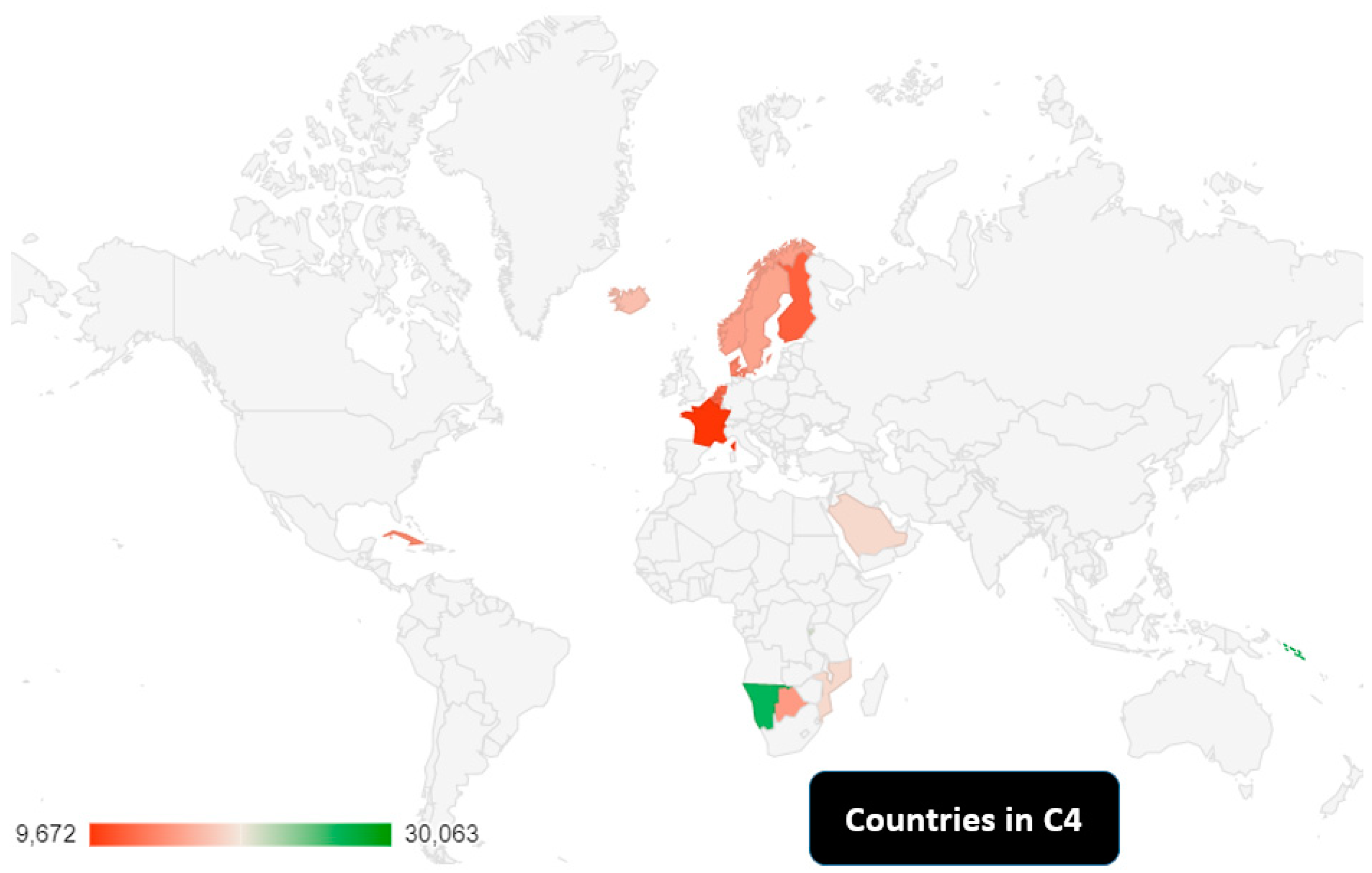
- Cluster 4: Svezia, Paesi Bassi, Danimarca, Namibia, Solomon Islands, Faroe Islands, Botswana, Iceland, Burundi, Aruba, Cuba, France, Finland, Belgium, Saudi Arabia, West Bank and Gaza, Seychelles, Mozambique, Brunei Darussalam, Norway. Cluster 4 countries are global leaders in terms of GEE value. C4 is constituted of a group of countries concentrated above all in Europe with the addition of Saudi Arabia, Cuba and some African countries. The Scandinavian countries have a long tradition of investment in the education and university system. France, Belgium and the Netherlands also have high levels of GEE. The fact that European countries have higher levels of GEE is counterfactual. In effect the level of GEE tends to be inversely associated to economic growth and high per-capita income. These European countries are an exception among countries with high GDP per capita. These countries have significantly benefited from the development of GEE. In fact, the economy of these European countries has efficiently acquired a hegemonic role in the context of the knowledge and innovation economy as demonstrated by the high ranks in terms of DESI score. Some considerations are necessary for the case of Cuba. Cuba is in fact an atypical case of a country with a low per capita income associated with a high level of human capital as demonstrated for example in the high professionalism achieved in the medical-pharmacological sector. The Cuban investment in education is a legacy of the communist regime of Fidel Castro who intended instruction as a force for the liberation of the people from oppression with significant benefits also for the national economy. The C4 countries are therefore leaders in terms of GEE for reasons related to the recognition of the strategic role of education for the development of the human capital and the promotion of economic growth at national level.
Figure 5.
Countries in C4.
5. Predictions and Machine Learning for the prediction of the Future Value of GEE
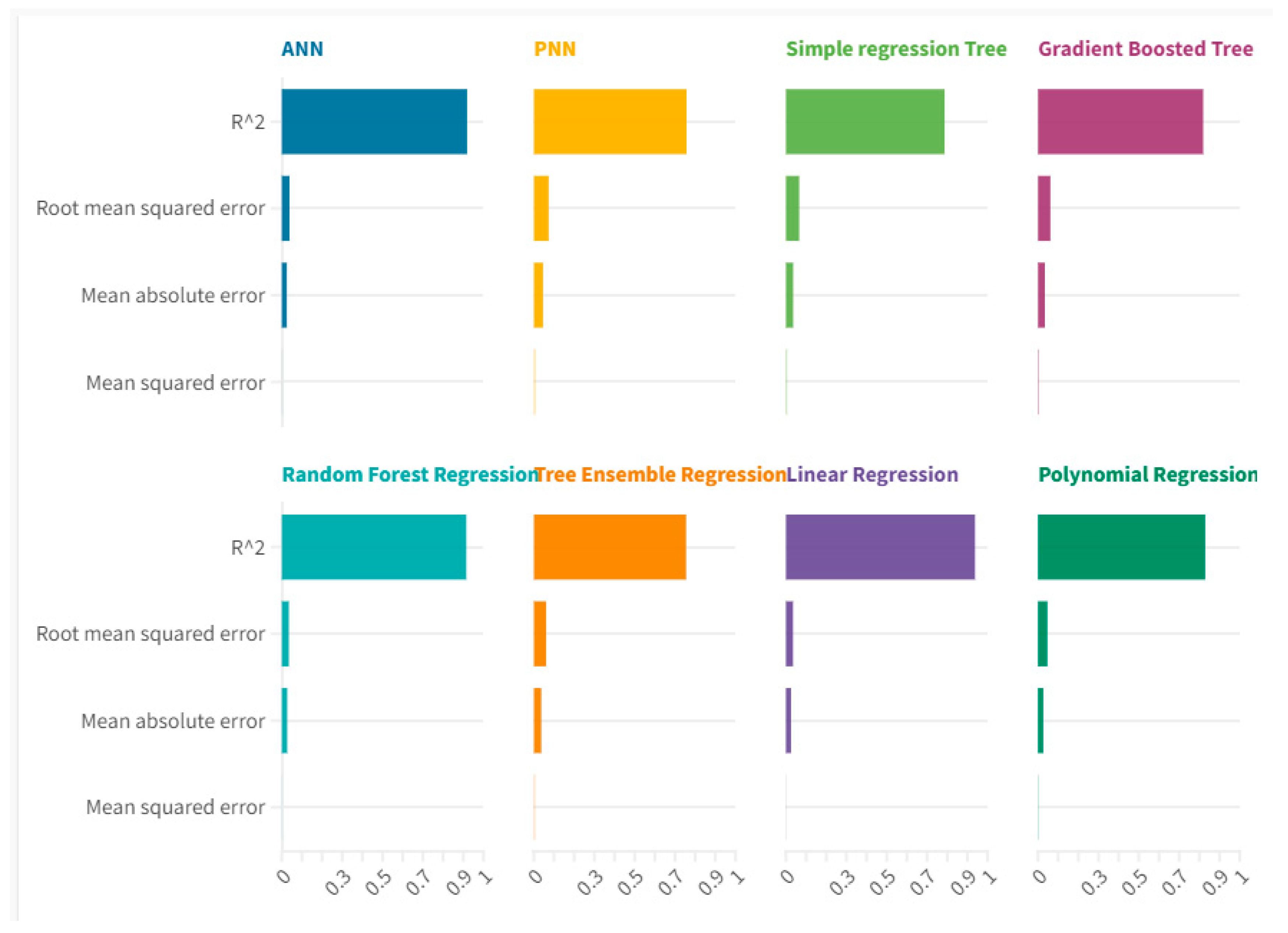
In the following analysis, we compare eight different machine-learning algorithms for predicting the future value of the amount of GEE. 70% of the data was used to train the algorithms and the remaining 30% was used for prediction. We have decided the most efficient algorithm to use based on a maximization of the R-Squared value and a minimization of the value of the statistical errors, i.e. MAE, RMSE, and MSE. Each algorithm has gained a score within the four classifications, one for each statistical indicator. The algorithm scores were summed. The algorithm that scored the lowest rank is the "Best Predictor".
The following ranking of the algorithms is therefore indicated, i.e.:
- Polynomial Regression with a payoff value equal to 4;
- Random Forest Regression with a payoff value equal to 11;
- Linear Regression with a payoff value equal to 12;
- Tree Ensemble Regression with a payoff value of 14;
- ANN-Artificial Neural Network with a payoff value of 21;
- Gradient Boosted Tree Regression with a payoff value of 23;
- Simple Regression Tree with a payoff value equal to 27;
- PNN-Probabilistic Neural Network with a payoff value of 32.
Based on our analysis the Polynomial Regression is the “Best Predictor”.
Figure 6.
Statistical Errors of the Machine Learning Algorithm used for the Prediction.
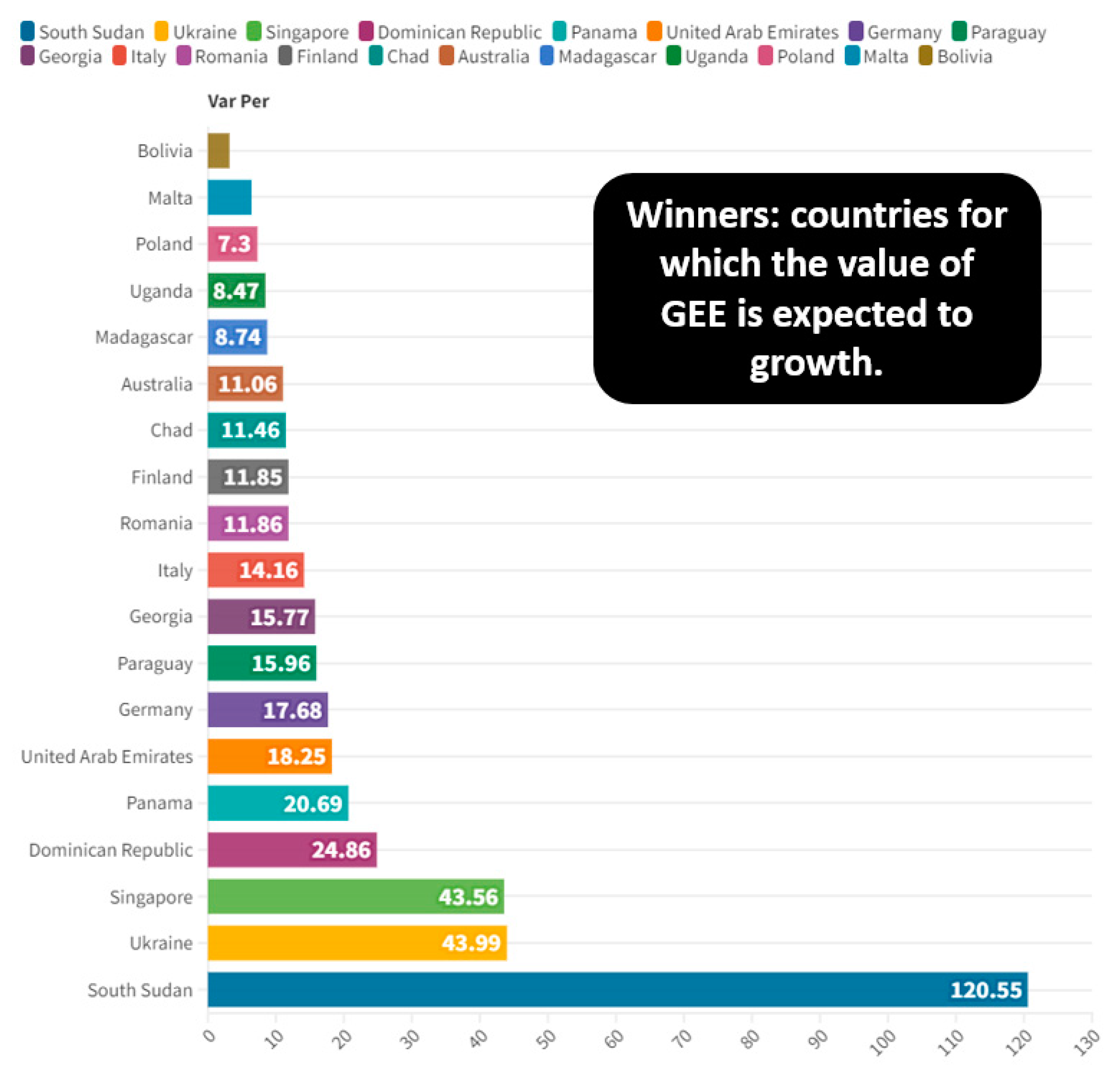
Through the application of the best predictor algorithm, i.e. the Polynomial Regression according to R-squared and statistical errors, it is possible to identify countries for which is predicted and increase in GEE, i.e. winners. With the same prediction it is possible to find countries for which the value of GEE is expected to decrease i.e. losers. Overall, by averaging between winners and losers countries, it appears that the mean value of GEE for the analysed countries is predicted to grow by 7.09%. If we consider winners countries in a ranking, then we found that South Sudan is in the first countries with an expected growth of GEE from 5.5 to 12.24 or equal to 6.69 equivalent to 120.55%. Ukraine is the second country with a variation from an amount of 13.09 up to 18.84 or equal to an amount of 5.76 units equal to 43.99%. Singapore is the third country with a variation from an amount of 11.81 up to 16.96 or equal to 5.15 equivalent to a value of 43.56%.
However, following the predictive analysis, it is also necessary to ask whether it is plausible that these countries have high growth rates in terms of GEE such as the ones we have identified. Indeed, we must answer this question positively. In fact, at least within the analysed countries, there do not seem to exist political and economic conditions that can limit the growth of GEE. In fact, considering the countries analysed, it is possible to verify that they are both countries with a low per capita income and countries with a high per capita income. Indeed, both types of countries have an interest in growth in terms of GEE. High per capita income countries have an interest in the growth of GEE to boost their performance in terms of knowledge economy, digitization and promote the high-tech sector. Countries with low per capita income need to increase the value of GEE to grow in per capita income, to increase the value of HDI and also promote the ability to attract Foreign Direct Investments-FDI in high value-added sectors.
Figure 7.
Winners: countries for which the value of GEE is expected to growth.
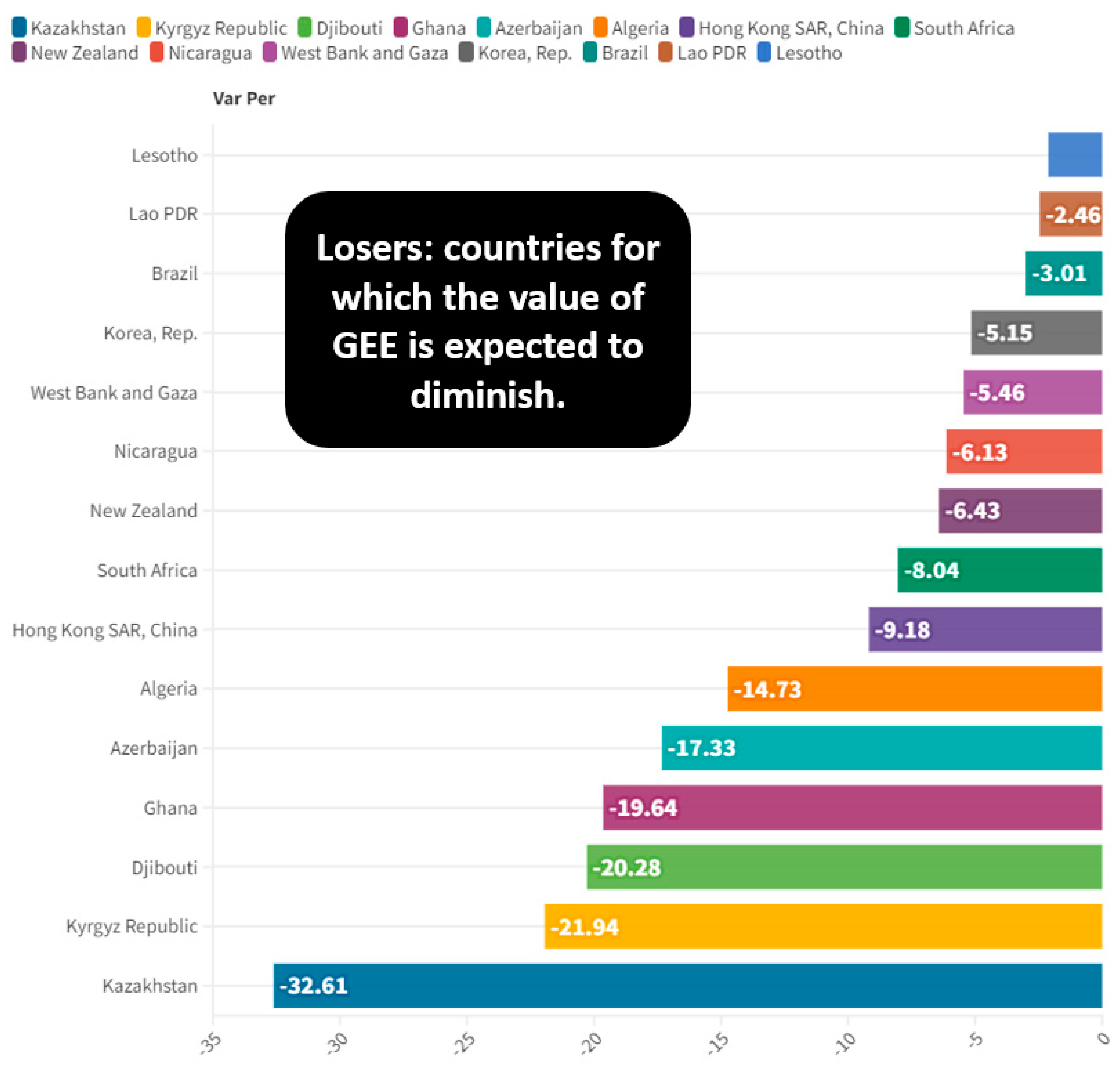
Among the losing countries, i.e. the countries that have a negative trend in terms of GEE in the first places, there are:
- Kazakhstan with a variation from 18.59% up to a value of 12.53% or equal to an amount of -6.06 units equivalent to -32.61%;
- Kyrgyz Republic with a variation from 20.69 up to an amount of 16.15 units or equal to a variation of -4.54 units equal to -21.94%;
- Djibouti with a variation from 14.28 up to a value of 12.53 or equal to -6.06 units equal to -32.61%.
Countries that are as losers in terms of GEE are also countries with low per capita income, with the exception of Hong Kong, South Korea, and New Zealand. Notwithstanding the numerical correctness of the prediction of the Polynomial Regression, we also must investigate if this prediction makes sense under an economic point of view, considering either the economic theory either the time series of the selected countries. The answer is yes, the prediction can be correct economically, but with the exceptions of Azerbaijan, Lesotho, and Lao. These countries have a low level of GEE compared to the other countries that are considered as losers. Since the value of GEE is already low, it is difficult for Azerbaijan, Lesotho, and Lao to further reduce its value. The value of GEE should instead increase for three reasons: first is already low and should achieve the average value of other similar countries, second the investment of GEE in low per capita income tends to be greater, third Azerbaijan, Lesotho and Lao would increase the value of GEE to gain the economic advantages of digitization and the profits of high-tech sectors.
Figure 8.
Losers: countries for which.
The aggregate value of GEE for the analysed countries is expected to grow on average of 7.09%. We have to investigate the economic meaning of the predicted value. We believe that the prediction makes sense on an economic point of view for two reasons:
- many countries among the predicted ones have low per capita income. These countries need to improve the level of GEE either to promote human capital either to trigger the economic development and growth;
- also high per capita income countries need to improve GEE to better afford the challenges of artificial intelligence, digitalization and to strengthen the high-tech sector.
For these reasons, we consider the prediction of the value of GEE obtained with the Polynomial Regression correct either on a statistical point of view either for their economic implications.
6. Conclusions
The dynamics of the GEE variable is positive in the context of ESG model. GEE tends to grow consistently with the ESG variables in an aggregate sense. But, if we make a decomposition of the single components of the ESG model, then we can observe some counterfactual results. GEE growth is positively associated with the E component within the ESG model is full i.e. GEE grows with environmental sustainability. The relationship between GEE and the G component of the ESG model is negative, that is, GEE grows in the worsening of G measured by GE. The relationship between GEE and the S component in the ESG model is both controversial both positive in a broad sense: in fact while on one side GEE growths with CD and UT, on the other side GEE decreases with HB.
The cluster analysis has showed the hegemony of Scandinavian countries in terms of GEE.
The prediction with Polynomial Regression, ranked as the best predictor, shows a positive trend in the future value of GEE, even if we have argued that the growth of GEE is underestimated for Azerbaijan, Lesotho, and Lao.
The role of education will be crucial in the fight for the hegemony within governance models. ESG models can acquire hegemony within governance only if universities will invest in creating ESG course in MBA programs. Policy makers should incentivize universities that are actively promote ESG models within their courses for economists and engineers.
Funding
The authors received no financial support for the research, authorship, and/or publication of this article.
Data Availability Statement
The data presented in this study are available on request from the corresponding author.
Acknowledgements
We are grateful to the teaching staff of the LUM University “Giuseppe Degennaro” and to the management of the LUM Enterprise s.r.l. for the constant inspiration to continue our scientific research work undeterred.
Conflicts of Interest
The authors declare that there is no conflict of interests regarding the publication of this manuscript. In addition, the ethical issues, including plagiarism, informed consent, misconduct, data fabrication and/or falsification, double publication.
Software
The authors have used the following software: Gretl for the econometric models, Orange for clusterization and network analysis, and KNIME for machine learning and predictions. They are all free version without licenses.
Appendix A
| ACRONYM | Variables | Definition |
| GEE | Government expenditure on education, total (% of government expenditure) | General government expenditure on education (current, capital, and transfers) is expressed as a percentage of total general government expenditure on all sectors (including health, education, social services, etc.). It includes expenditure funded by transfers from international sources to government. General government usually refers to local, regional and central governments. |
| GE | Government Effectiveness | Government Effectiveness captures perceptions of the quality of public services, the quality of the civil service and the degree of its independence from political pressures, the quality of policy formulation and implementation, and the credibility of the government's commitment to such policies. Estimate gives the country's score on the aggregate indicator, in units of a standard normal distribution, i.e. ranging from approximately -2.5 to 2.5. |
| CD | Cause of death, by communicable diseases and maternal, prenatal and nutrition conditions (% of total) | Cause of death refers to the share of all deaths for all ages by underlying causes. Communicable diseases and maternal, prenatal and nutrition conditions include infectious and parasitic diseases, respiratory infections, and nutritional deficiencies such as underweight and stunting. |
| EU | Energy use (kg of oil equivalent per capita) | Energy use refers to use of primary energy before transformation to other end-use fuels, which is equal to indigenous production plus imports and stock changes, minus exports and fuels supplied to ships and aircraft engaged in international transport. |
| FPI | Food production index (2014-2016 = 100) | Food production index covers food crops that are considered edible and that contain nutrients. Coffee and tea are excluded because, although edible, they have no nutritive value. |
| HB | Hospital beds (per 1,000 people) | Hospital beds include inpatient beds available in public, private, general, and specialized hospitals and rehabilitation centers. In most cases beds for both acute and chronic care are included. |
| TMPA | Terrestrial and marine protected areas (% of total territorial area) | Terrestrial protected areas are totally or partially protected areas of at least 1,000 hectares that are designated by national authorities as scientific reserves with limited public access, national parks, natural monuments, nature reserves or wildlife sanctuaries, protected landscapes, and areas managed mainly for sustainable use. Marine protected areas are areas of intertidal or subtidal terrain--and overlying water and associated flora and fauna and historical and cultural features--that have been reserved by law or other effective means to protect part or all of the enclosed environment. Sites protected under local or provincial law are excluded. |
| UT | Unemployment, total (% of total labor force) (modeled ILO estimate) | Unemployment refers to the share of the labor force that is without work but available for and seeking employment. |
| WLS, using 813 observations | |||||
| Included 98 cross-sectional units | |||||
| Dependent variable: A28 | |||||
| Weights based on per-unit error variances | |||||
| Coefficient | Std. Error | t-ratio | p-value | ||
| const | 2.40949 | 0.333971 | 7.215 | <0.0001 | *** |
| l_A27 | −0.452850 | 0.095417 | −4.746 | <0.0001 | *** |
| A9 | 0.186039 | 0.040533 | 4.59 | <0.0001 | *** |
| A19 | 0.000286 | 5.95E-05 | 4.801 | <0.0001 | *** |
| A21 | 0.074814 | 0.005175 | 14.46 | <0.0001 | *** |
| A30 | −0.400849 | 0.056986 | −7.034 | <0.0001 | *** |
| A64 | 0.080339 | 0.017349 | 4.631 | <0.0001 | *** |
| A65 | 0.057553 | 0.026946 | 2.136 | 0.033 | ** |
| Statistics based on the weighted data: | ||||
| Sum squared resid | 771.393 | S.E. of regression | 0.9789 | |
| R-squared | 0.49136 | Adjusted R-squared | 0.48694 | |
| F(7, 805) | 111.094 | P-value(F) | 1.1e-113 | |
| Log-likelihood | −1132.242 | Akaike criterion | 2280.48 | |
| Schwarz criterion | 2318.09 | Hannan-Quinn | 2294.92 | |
| Statistics based on the original data: | ||||
| Mean dependent var | 8.90255 | S.D. dependent var | 7.59439 | |
| Sum squared resid | 40598.5 | S.E. of regression | 7.10161 | |
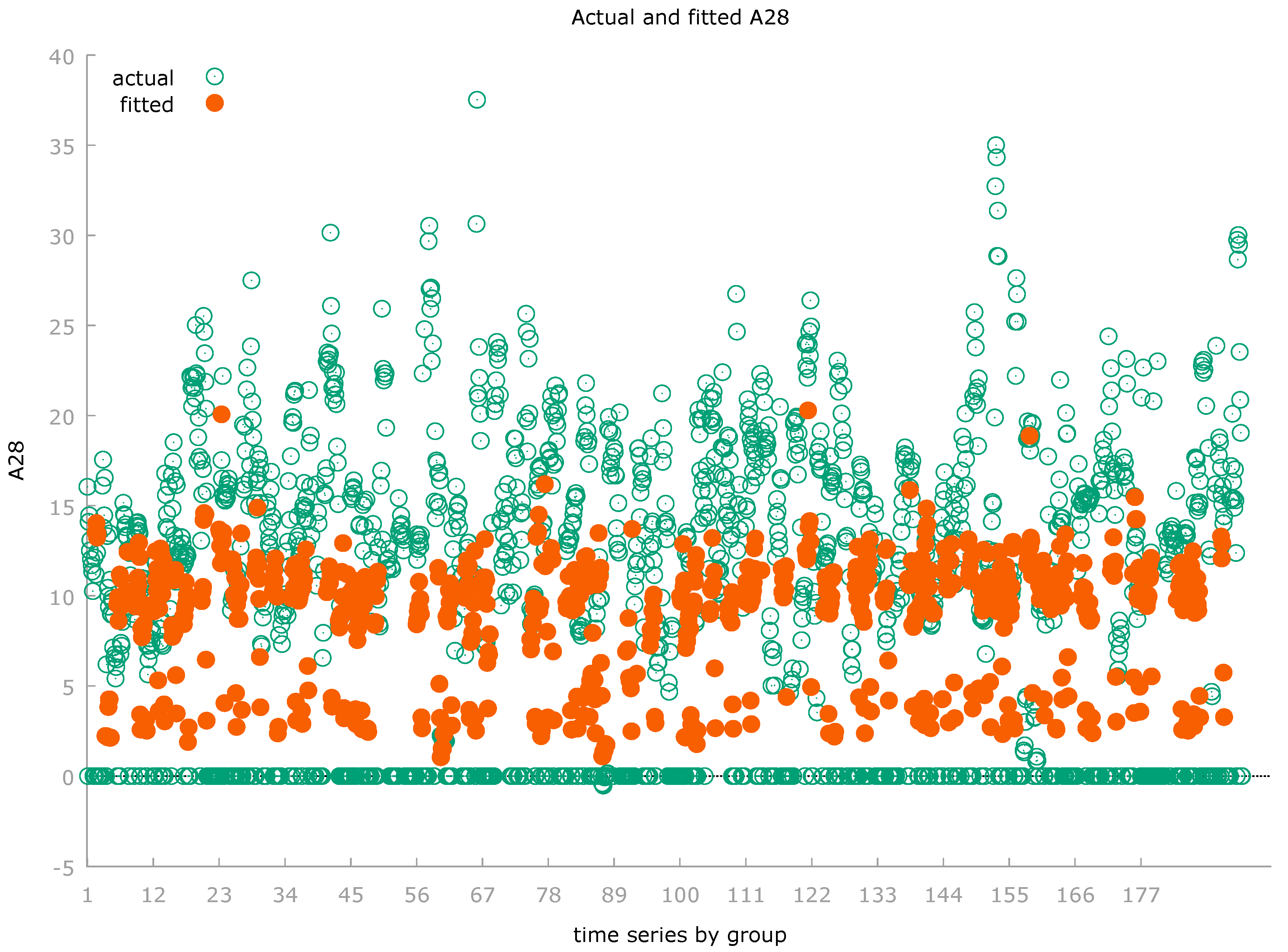
| Pooled OLS, using 813 observations | |||||
| Included 98 cross-sectional units | |||||
| Time-series length: minimum 1, maximum 10 | |||||
| Dependent variable: A28 | |||||
| Coefficient | Std. Error | t-ratio | p-value | ||
| const | 3.59150 | 0.612142 | 5.867 | <0.0001 | *** |
| l_A27 | −0.470012 | 0.210636 | −2.231 | 0.0259 | ** |
| A9 | 0.188949 | 0.0477061 | 3.961 | <0.0001 | *** |
| A19 | 0.000272386 | 9.89854e-05 | 2.752 | 0.0061 | *** |
| A21 | 0.0576490 | 0.00718759 | 8.021 | <0.0001 | *** |
| A30 | −0.521217 | 0.106855 | −4.878 | <0.0001 | *** |
| A64 | 0.111356 | 0.0297857 | 3.739 | 0.0002 | *** |
| A65 | 0.0910787 | 0.0426087 | 2.138 | 0.0329 | ** |
| Pooled OLS, using 813 observations | |||||
| Included 98 cross-sectional units | |||||
| Time-series length: minimum 1, maximum 10 | |||||
| Dependent variable: A28 | |||||
| Coefficient | Std. Error | t-ratio | p-value | ||
| const | 3.5915 | 0.61214 | 5.867 | <0.0001 | *** |
| l_A27 | −0.470012 | 0.21064 | −2.231 | 0.0259 | ** |
| A9 | 0.18895 | 0.04771 | 3.961 | <0.0001 | *** |
| A19 | 0.00027 | 9.90E-05 | 2.752 | 0.0061 | *** |
| A21 | 0.05765 | 0.00719 | 8.021 | <0.0001 | *** |
| A30 | −0.521217 | 0.10686 | −4.878 | <0.0001 | *** |
| A64 | 0.11136 | 0.02979 | 3.739 | 0.0002 | *** |
| A65 | 0.09108 | 0.04261 | 2.138 | 0.0329 | ** |
| Mean dependent var | 8.90255 | S.D. dependent var | 7.59439 |
| Sum squared resid | 39931.7 | S.E. of regression | 7.04306 |
| R-squared | 0.14734 | Adjusted R-squared | 0.13992 |
| F(7, 805) | 19.8718 | P-value(F) | 1.17E-24 |
| Log-likelihood | −2736.587 | Akaike criterion | 5489.18 |
| Schwarz criterion | 5526.78 | Hannan-Quinn | 5503.61 |
| rho | 0.739 | Durbin-Watson | 0.45908 |
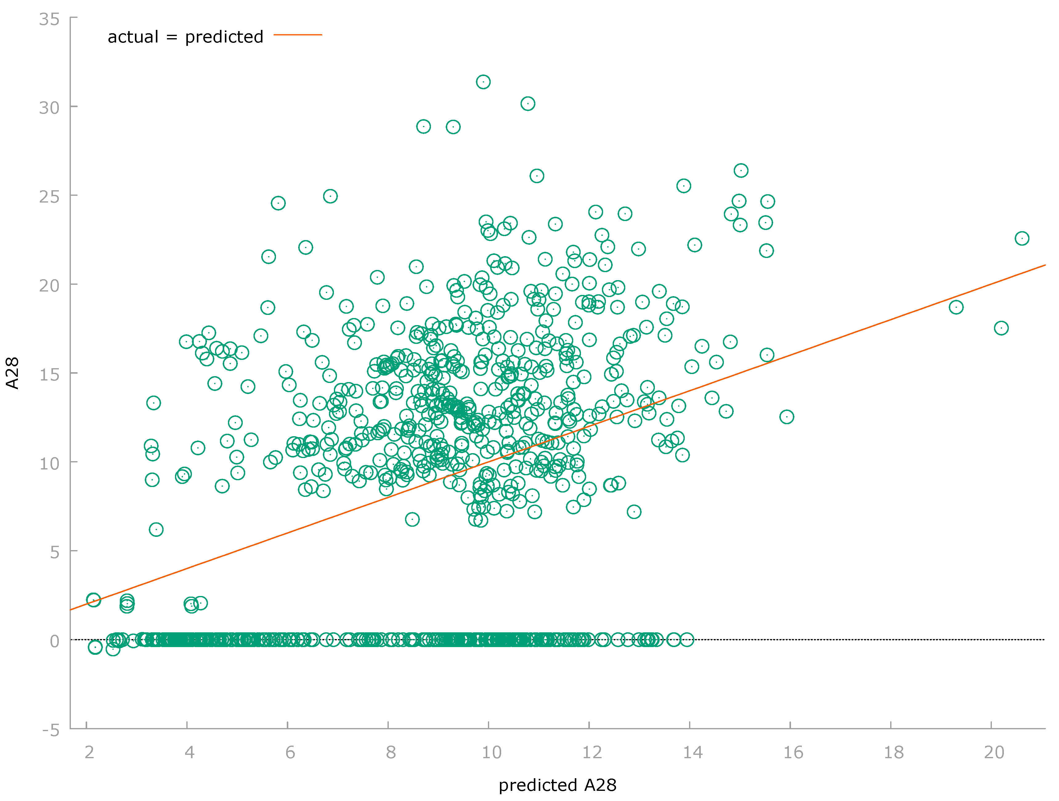
| Fixed-effects, using 813 observations | |||||
| Included 98 cross-sectional units | |||||
| Time-series length: minimum 1, maximum 10 | |||||
| Dependent variable: A28 | |||||
| Coefficient | Std. Error | t-ratio | p-value | ||
| const | 1.57607 | 0.780996 | 2.018 | 0.0440 | ** |
| l_A27 | −1.43833 | 0.333918 | −4.307 | <0.0001 | *** |
| A9 | 0.112728 | 0.0334793 | 3.367 | 0.0008 | *** |
| A19 | 0.000434257 | 7.92061e-05 | 5.483 | <0.0001 | *** |
| A21 | 0.0302943 | 0.00579020 | 5.232 | <0.0001 | *** |
| A30 | 0.369312 | 0.126930 | 2.910 | 0.0037 | *** |
| A64 | 0.136674 | 0.0223691 | 6.110 | <0.0001 | *** |
| A65 | 0.256559 | 0.0917394 | 2.797 | 0.0053 | *** |
| Fixed-effects, using 813 observations | |||||
| Included 98 cross-sectional units | |||||
| Time-series length: minimum 1, maximum 10 | |||||
| Dependent variable: A28 | |||||
| Coefficient | Std. Error | t-ratio | p-value | ||
| const | 1.57607 | 0.781 | 2.018 | 0.044 | ** |
| l_A27 | −1.43833 | 0.33392 | −4.307 | <0.0001 | *** |
| A9 | 0.11273 | 0.03348 | 3.367 | 0.0008 | *** |
| A19 | 0.00043 | 7.92E-05 | 5.483 | <0.0001 | *** |
| A21 | 0.03029 | 0.00579 | 5.232 | <0.0001 | *** |
| A30 | 0.36931 | 0.12693 | 2.91 | 0.0037 | *** |
| A64 | 0.13667 | 0.02237 | 6.11 | <0.0001 | *** |
| A65 | 0.25656 | 0.09174 | 2.797 | 0.0053 | *** |
| Mean dependent var | 8.902553 | S.D. dependent var | 7.594386 |
| Sum squared resid | 14903.52 | S.E. of regression | 4.588047 |
| LSDV R-squared | 0.681765 | Within R-squared | 0.265324 |
| LSDV F(104, 708) | 14.58435 | P-value(F) | 7.60E-120 |
| Log-likelihood | −2335.952 | Akaike criterion | 4881.904 |
| Schwarz criterion | 5375.48 | Hannan-Quinn | 5071.369 |
| rho | 0.355801 | Durbin-Watson | 1.116093 |
| test on named regressors - |
| Test statistic: F(7, 708) = 36.5272 |
| with p-value = P(F(7, 708) > 36.5272) = 1.05213e-43 |
| Test for differing group intercepts - |
| Null hypothesis: The groups have a common intercept |
| Test statistic: F(97, 708) = 12.2575 |
| with p-value = P(F(97, 708) > 12.2575) = 1.13564e-99 |
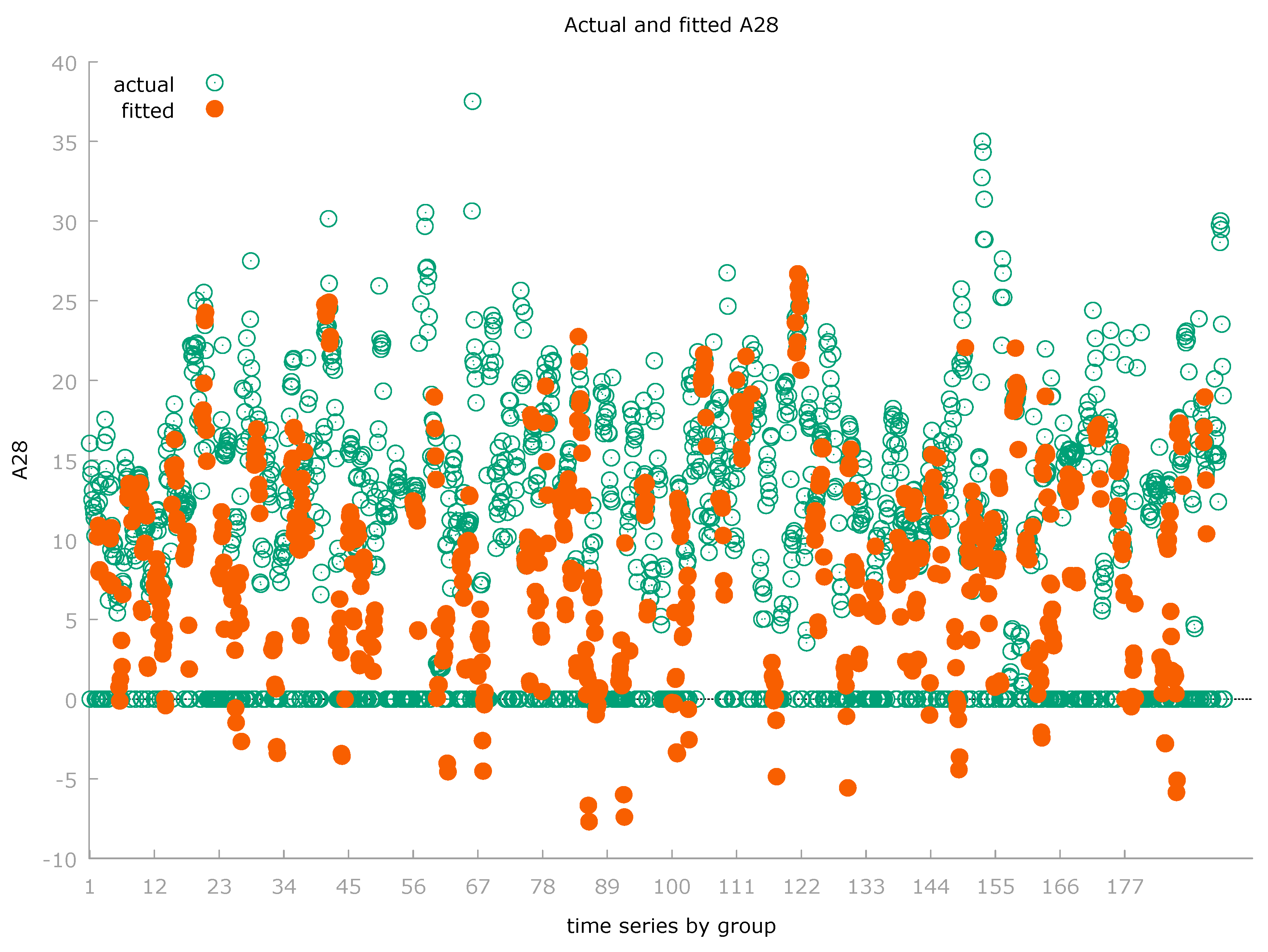
| Random-effects (GLS), using 813 observations | |||||
| Included 98 cross-sectional units | |||||
| Time-series length: minimum 1, maximum 10 | |||||
| Dependent variable: A28 | |||||
| Coefficient | Std. Error | z | p-value | ||
| const | 2.29877 | 0.83854 | 2.741 | 0.0061 | *** |
| l_A27 | −1.14585 | 0.26754 | −4.283 | <0.0001 | *** |
| A9 | 0.11812 | 0.03355 | 3.521 | 0.0004 | *** |
| A19 | 0.00043 | 7.86E-05 | 5.464 | <0.0001 | *** |
| A21 | 0.03538 | 0.00566 | 6.252 | <0.0001 | *** |
| A30 | 0.19514 | 0.11686 | 1.67 | 0.0949 | * |
| A64 | 0.12955 | 0.0222 | 5.835 | <0.0001 | *** |
| A65 | 0.16998 | 0.06812 | 2.495 | 0.0126 | ** |
| Mean dependent var | 8.90255 | S.D. dependent var | 7.59439 |
| Sum squared resid | 43019 | S.E. of regression | 7.30571 |
| Log-likelihood | −2766.860 | Akaike criterion | 5549.72 |
| Schwarz criterion | 5587.33 | Hannan-Quinn | 5564.16 |
| rho | 0.3558 | Durbin-Watson | 1.11609 |
| 'Between' variance = 28.2612 |
| 'Within' variance = 21.0502 |
| mean theta = 0.687986 |
| Joint test on named regressors - |
| Asymptotic test statistic: Chi-square(7) = 236.57 |
| with p-value = 1.99231e-47 |
| Breusch-Pagan test - |
| Null hypothesis: Variance of the unit-specific error = 0 |
| Asymptotic test statistic: Chi-square(1) = 908.437 |
| with p-value = 1.43822e-199 |
| Hausman test - |
| Null hypothesis: GLS estimates are consistent |
| Asymptotic test statistic: Chi-square(7) = 31.1548 |
| with p-value = 5.82155e-05 |
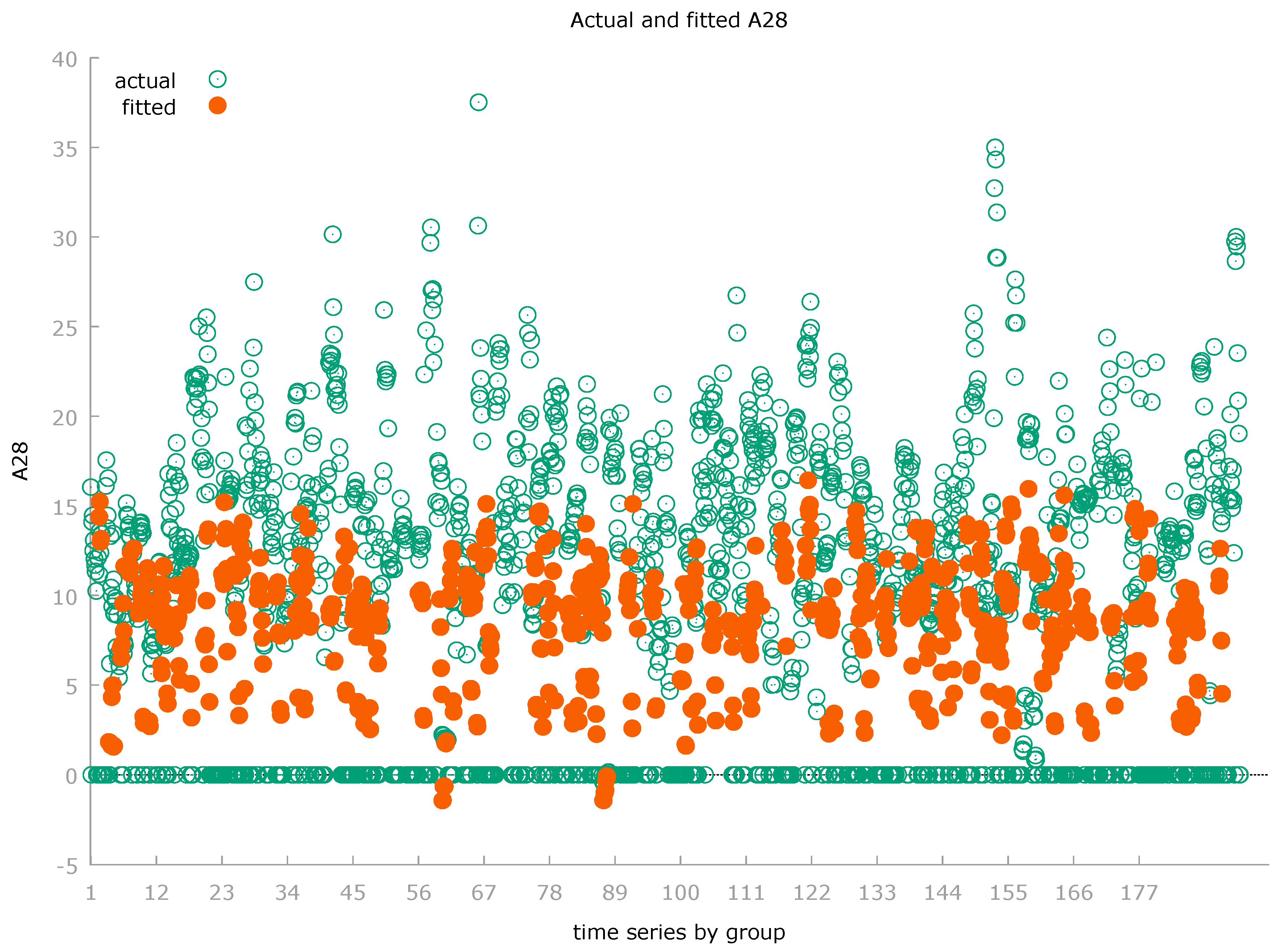
Clusterization
References
- G. Ferri e A. Leogrande, «The Founding Role of Cooperative Banking Within the European Variety of Capitalism,» in Contemporary Trends in European Cooperative Banking: Sustainability, Governance, Digital Transformation, and Health Crisis Response, Springer International Publishing, Cham, 2022, pp. 29-54.
- G. Ferri e A. Leogrande, «Stakeholder Management, Cooperatives, and Selfish-Individualism,» Journal for Markets and Ethics, vol. 9, n. 2, pp. 61-75, 2021.
- G. Ferri e A. Leogrande, «Entrepreneurial Pluralism,» The Oxford Handbook of Mutual, Co-Operative, and Co-Owned Business , vol. 28, n. 4, pp. 295-303, 2017. [CrossRef]
- G. Ferri e A. Leogrande, «Was the Crisis Due to a Shift from Stakeholder to Shareholder Finance? Surveying the Debate,» Euricse , n. 1576, 2015.
- Costantiello e A. Leogrande, «The Determinants of CO2 Emissions in the Context of ESG Models at World Level,» SSRN , n. 4425121, 2023.
- Leogrande e A. Costantiello, «The Role of GDP Growth in the ESG Approach at World Level,» SSRN, 2023.
- Costantiello e A. Leogrande, «The Ease of Doing Business in the ESG Framework at World Level,» SSRN , n. 4420946, 2023.
- Costantiello e A. Leogrande, «The Impact of Research and Development Expenditures on ESG Model in the Global Economy,» Center for Open Science, n. 85v3f, 2023.
- Costantiello e A. Leogrande, «The Role of Political Stability in the Context of ESG Models at World Level,» 2023.
- Costantiello e A. Leogrande, «The Impact of Voice and Accountability in the ESG Framework in a Global Perspective,» SSRN , n. 4398483, 2023.
- Costantiello e A. Leogrande, «The Regulatory Quality and ESG Model at World Level,» SSRN , n. 4388957, 2023.
- Leogrande, «The Rule of Law in the ESG Framework in the World Economy,» SSRN , n. 4355016, 2023.
- L. Laureti, A. Costantiello e A. Leogrande, «The Role of Government Effectiveness in the Light of ESG Data at Global Level,» SSRN , n. 4324938, 2023.
- L. Laureti, A. Costantiello e A. Leogrande, «The Fight Against Corruption at Global Level. A Metric Approach,» University Library of Munich, Germany, n. 115837, 2022.
- L. Laureti, A. Costantiello e A. Leogrande, «The Role of Renewable Energy Consumption in Promoting Sustainability and Circular Economy. A Data-Driven Analysis,» 2022.
- L. Laureti, A. Massaro, A. Costantiello e A. Leogrande, «The Impact of Renewable Electricity Output on Sustainability in the Context of Circular Economy: A Global Perspective,» Sustainability, vol. 3, n. 2160, p. 15, 2023. [CrossRef]
- J. Kutzschbach, I. Peetz, P. Tanikulova e K. Willers, «How CEO’s education impacts CSR performance–An empirical analysis of publicly listed companies in Germany,» Management Studies, vol. 10, n. 3, pp. 50-63, 2020.
- T. Yao, «ESG Education and Job Choice,» Working paper, 2022.
- M. A. Ramadhan, R. Mulyany e E. Mutia, «The irrelevance of R&D intensity in the ESG disclosure? Insights from top 10 listed companies on global Islamic indices,» Cogent Business & Management, vol. 1, n. 2187332, p. 10, 2023. [CrossRef]
- W. Ghardallou, «Corporate sustainability and firm performance: the moderating role of CEO education and tenure,» Sustainability, vol. 6, n. 3513, p. 14, 2022. [CrossRef]
- H. T. Liao, C. L. Pan e Y. Zhang, «Collaborating on ESG consulting, reporting, and communicating education: Using partner maps for capability building design,» Frontiers in Environmental Science, vol. 11, n. 298, 2023. [CrossRef]
- P. JÍLKOVÁ e L. KNIHOVÁ, «ESG FACTORS IN SUSTAINABILITY REPORTING AS A COMPETITIVE ADVANTAGE».
- P. Dmuchowski, W. Dmuchowski, A. H. Baczewska-Dąbrowska e B. Gworek, «Environmental, social, and governance (ESG) model; impacts and sustainable investment–Global trends and Poland's perspective,» Journal of Environmental Management, vol. 329, n. 117023, 2023. [CrossRef]
- R. Sun, «Female leadership and corporate ESG performance: evidence from China,» Doctoral dissertation, University of Chicago, 2022.
- Passas, K. Ragazou, E. Zafeiriou, A. Garefalakis e C. Zopounidis, «ESG Controversies: A Quantitative and Qualitative Analysis for the Sociopolitical Determinants in EU Firms,» Sustainability, vol. 19, n. 12879, p. 14, 2022. [CrossRef]
- W. Shaw, «Relationship between Female Board Changes and ESG Scores with CSR Influences,» Doctoral dissertation, Capella University, 2022.
- P. B. Huang, C. C. Yang, M. M. W. Inderawati e R. Sukwadi, «Using Modified Delphi Study to Develop Instrument for ESG Implementation: A Case Study at an Indonesian Higher Education Institution,» Sustainability, vol. 19, n. 12623, p. 14, 2022. [CrossRef]
- V. Esteves-Miranda, W. Liao, E. Abington-Prejean e C. Parker, «Incorporating ESG Strategy in DEI for Leadership Roles in Higher Education,» American International Journal of Business Management (AIJBM), 2020.
- Clément, É. Robinot e L. Trespeuch, «Improving ESG Scores with Sustainability Concepts,» Sustainability, vol. 20, n. 13154, p. 14, 2022. [CrossRef]
- T. F. Cojoianu, A. G. Hoepner e Y. Lin, «Private market impact investing firms: Ownership structure and investment style,» International Review of Financial Analysis, vol. 84, n. 102374, 2022. [CrossRef]
- Sullivan, «A BRICS Currency Could Shake the Dollar’s Dominance. De-dollarization’s moment might finally be here,» Foreign Policy, n. https://foreignpolicy.com/2023/04/24/brics-currency-end-dollar-dominance-united-states-russia-china/, 2023.
Disclaimer/Publisher’s Note: The statements, opinions and data contained in all publications are solely those of the individual author(s) and contributor(s) and not of MDPI and/or the editor(s). MDPI and/or the editor(s) disclaim responsibility for any injury to people or property resulting from any ideas, methods, instructions or products referred to in the content. |
© 2023 by the authors. Licensee MDPI, Basel, Switzerland. This article is an open access article distributed under the terms and conditions of the Creative Commons Attribution (CC BY) license (http://creativecommons.org/licenses/by/4.0/).
Copyright: This open access article is published under a Creative Commons CC BY 4.0 license, which permit the free download, distribution, and reuse, provided that the author and preprint are cited in any reuse.


