
Submitted:
01 May 2023
Posted:
02 May 2023
You are already at the latest version
Abstract
We analyze the question of GDP Growth-GDPG rate in the context of Environmental, Social and Governance-ESG framework. We use World Bank data for 193 countries in the period 2011-2020 using different econometric techniques i.e., Panel Data with Fixed Effects, Panel Data with Random Effects, Pooled Ordinary Least Squares-OLS. We found that GDPG rate is positively associated, among others, to “Government Effectiveness” and “Prevalence of Undernourishment” and negatively associated among others to “Unemployment” and “Research and Development Expenditure”. Furthermore, we have applied the k-Means algorithm optimized with the Elbow method and we found the presence of four clusters in the sense of GDPG rate. Finally, we confront eight machine learning algorithms to predict the value of GDPG rate and we found that the Polynomial Regression is the best predictor. The Polynomial Regression predicts an increase of GDPG rate equal to 2.88% on average for the analysed countries.
Keywords:
Analysis of Collective Decision-Making
; General
; Political Processes: Rent-Seeking
; Lobbying
; Elections
; Legislatures
; and Voting Behaviour
; Bureaucracy
; Administrative Processes in Public Organizations
; Corruption
; Positive Analysis of Policy Formulation
; Implementation.
1. Introduction-Research Question
In the following article we consider the connection between GDPG and variables of the ESG model. Economists have deeply analyzed the causes for economic growth. However, the relationship between GDP and ESG variables is not yet clear. Here is the original contribution of our article that aims to investigate the relationship between the trend of economic growth and ESG model at world level. At the theoretical level we expect to discover a negative relationship between GDPG trend and ESG variables. And in fact, the dynamics of the GDP seems to be inconsistent with the determinants of the ESG model. At least for environmental issues [1], [2], [3]. In fact, increasing GDP means increasing energy consumption and therefore having a negative impact in terms of respect for the environment. emissions tend to grow with the value of GDPG especially for African and Asian countries. However, the theoretical positive connection between the G [4], [5], [6], [7], [8], [9] and S component of the ESG model and the GDPG appears more plausible. Furthermore, the ESG model has also an impact on entrepreneurship [10] and R&D at country level [11].
The article continues as follows: the second section presents a brief analysis of the literature, the third paragraph contains the econometric analysis, the fourth section show the result of the clusterization with the application of the k-Means algorithm, the fifth section compares the performance of eight machine learning algorithms for the prediction of the future value of GDPG, the sixth paragraph concludes. The appendix contains further statistical results.
2. Literature Review
A brief analysis of literature is presented below. The short analysis does not want to be exhaustive of the field. Instead, it has the unique end to introduce the theme of the relationship between ESG and GDPG in the light of the metric analysis that will be presented in sections three, four and five. We have reported a list of econometric articles in which the results show the complex relationship that exist between three components of the ESG model and GDPG.
ESG and GDP. The relationship between the application of ESG models and the trend of GDP is paradoxical. In fact, the ESG models have been proposed above all in high-capita countries. However, there are significant differences between the various western countries in terms of effective ESG-GDPG relationship. The econometric and empirical results of the cited articles show the presence of a positive relationship between ESG and GDPG in the USA while this relationship seems to be negative in Europe. Furthermore, if on the one hand the S and G component are positively associated with GDPG, while the E component in the ESG model tends to be negatively associated with GDPG. In fact, one of the determinants of economic growth consists in the consumption of energy which inevitably generates an increase in the value of emissions. It follows that environmental sustainability tends to be a challenge for high GDPG countries.
Among the ESG variables only G seems not to have a negative effect on financial stability in the case of a reduction in GDPG rate for companies listed in the S&P 500 [12]. The positive relationship between GDP and ESG scores holds at global level [13]. ESG either Granger causes GDP either is Granger caused by GDP in OECD countries in the period 2000-2017 [14]. For countries that have a medium-low level of GDP there is a positive impact of the adoption of ESG models in implementing the energy transition [15]. Financial development, ESG scores and GDP are positively associated in Asian countries in the period 2013-2017 [16]. There is a negative relationship between GDPG rates and ESG scores in 25 OECD countries in the period 2008-2019 [17]. Financial investments in ESG projects are positively associated to economic growth in Latin America countries [18]. There is a positive relationship between GDPG rate and emissions suggesting that the E component of the ESG model does not improve the economic growth [19]. In EU there is a negative relationship between ESG and GDPG [20].
ESG and GDP in banking. The ESG type models have been applied widely in the banking system. Two different type of governance models have been juxtaposed in the banking sector i.e. stakeholder oriented governance and shareholder-oriented governance [21]. The affirmation of the ESG model tends to be the conclusion of a long debate that starting from the Corporate Social Responsibility has led to the recognition of social, governance and environmental issues within bank governance [22]. The relevance of social, ethical, and environmental issues in banking system can be traced back to the foundation of European cooperative banks [23]. There is a positive relationship between GDP and ESG scores in USA countries, even if the same relationship turns negative in the case of Europe [24]. ESG scores in banking tend to be higher in countries with low GDP [25]. The impact of ESG models on shareholder value creation is negatively associated to GDP in a set of 166 banks for 31 countries in the period 2010-2015 [26]. ESG and GDP are positively and insignificantly associated in the West Africa banking sector [27].
ESG and GDP and corporations. The application of ESG model within the governance of the corporations is a strategy that fulfils a set of purposes. Large companies apply ESG model to obtain greater reputation among consumers and investors by showing sensitivity towards ethical, social, and environmental issues. Since many financers are interested in offering resources for ESG based projects then a new form of free riding arose i.e., greenwashing. There is a positive relationship between the adoption of ESG models and practices at firm level and the increase in GDP per capita, a condition that reveals the existence of deep connection between micro-economic decision making and macro-economic performance [28]. There is a positive relationship between higher ESG scores and GDP values in the MSCI ESG database for the period 2007-2017 [29]. The impact of macro-economic uncertainty on ESG model is negatively associated to GDPG in a set of companies in China, USA, and UK [30].
ESG and GDP during the Covid 19 pandemic. During the Covid 19 pandemic, GDP has been negatively associated to the environmental component of the ESG score, negatively associated to the social component of ESG score, positively associated to the governance component of ESG score, and negatively associated to the overall ESG score [31].
3. The Econometric Model for the Estimation of the Value of GDPG
We present an econometric analysis using the following models or: Panel Data with Fixed Effects, Panel Data with Random Effects, Poled Ordinary Least Squares-OLS. Specifically, we have estimated the following equation or:
where and .
We found that the level of GDPG rate is positively associated to:
- GE: is a variable that considers the perceptions of the quality of public services, the quality of the civil service and the degree of independence from political pressure, the quality of the formulation and implementation of policies and the credibility of the government’s commitment to these policies The estimate provides the score of the country on the aggregate indicator, in units of a standard distribution, that is to say they range from about -2.5 to 2.5. There is a positive relationship between the value of GDPG and the value of GE. The motivation consists in the fact that the countries that have a public system that offers efficient services also have a positive GDPG trend. There is therefore no contrast between the development of the public sector and the development of the private sector. Indeed, on the contrary, the ability to develop the public economy is positively associated with GDPG.
- PU: is the percentage of the population whose habitual food consumption is insufficient to try the dietary energy levels that are required to maintain a normal active and healthy life. There is a positive relationship between PU value and the value of GDPG. This positive relationship is since the countries that grow most have reduced pro-capita incomes and therefore high values in terms of PU high as for example in the case of Bangladesh, Dominican Republic, Ethiopia, Ghana, Guinea, Malawi. However, this positive relationship tends to disappear if we consider the growth of the GDP in an absolute sense or per capita income. In fact, if there is an increase in the GDP per capita then the value of PU value tends to decrease. Although in the event of growth of the absolute pro-capita, the GDPG value would decrease, as the countries that have high per-capita incomes tend to have a reduced GDPG.
- NRD: is a variable that measures the exhaustion of natural resources is the sum of the exhaustion of the net forest, the exhaustion of energy and mineral exhaustion. There is a positive relationship between NRD and GDPG. This positive relationship is due to the fact that many countries that have high levels of GDPG are also countries that use large amount of natural resources to support economic growth. In fact, to promote economic growth, it is necessary improve the consumption of natural and energy resources with also negative effects in terms of emissions. It follows that countries that grow more in terms of GDP are also countries that have high values in terms of NRD.
- AE: is the percentage of population with access to electricity. Electrification data are collected from industry, national surveys, and international sources. There is a positive relationship between AE and GDPG. The countries that grow more in terms of GDPG also have a higher consumption of AE. In fact, to have a greater GDPG it is necessary that industries produce more. The growth of industrial production requires growth in electricity consumption. The consumption of electricity requires a growth in the distribution of the electrical network, and the increase in the percentage of the population that have access to electricity. In addition, it should be considered that a significant part of GDP is the consumption of families and individuals. The growth of electrification increases the level of consumption with a positive impact in terms of GDPG.
- FPI: covers food crops that are considered edible and that contain nutrients. Coffee and tea are excluded because, although edible, they have no nutritional value. There is a positive relationship between the FPI and GDPG. This relationship is since many of the countries that have high GDPG rates are also countries that have high levels of food production such as Senegal with 181.51, Mongolia with 173.71, Guinea with 135.81, the Tajikistan with 135.55, Mali with 134.57, Malawi with 132.97. Countries with high rates of economic growth are often countries with low per capita income, i.e. developing countries. In developing countries, the percentage of GDP deriving from agriculture tends to be high, in contrast to countries with a high GDP which focus more on the services sector.
- NOE: are emissions from agricultural biomass burning, industrial activities, and livestock management. There is a positive relationship between NOE and GDPG. The countries that grow more from an economic point of view also tend to have higher levels of pollution deriving from the industrial production systems. It therefore derives a growth of values also in terms of NOE. Among the countries that produce the greatest value of NOE there are at the top of Mongolia with 4.3, New Zealand with 3.0, Cameron and Australia with 2.4, and Uruguay with 2.3. The positive relationship between high levels of GDPG and high levels of NOE raises significant issues that refer to the relationship between ethics and the environment. Many of the environmental economic policies generate deleterious effects on low per-capita income countries by preventing them from growing in GDP. If higher GDPG rates are positively associated to pollution then the imposition of environmental constraints can reduce the ability of poor countries to develop their economy.
Figure 1.
Average value of the estimations with regressions.
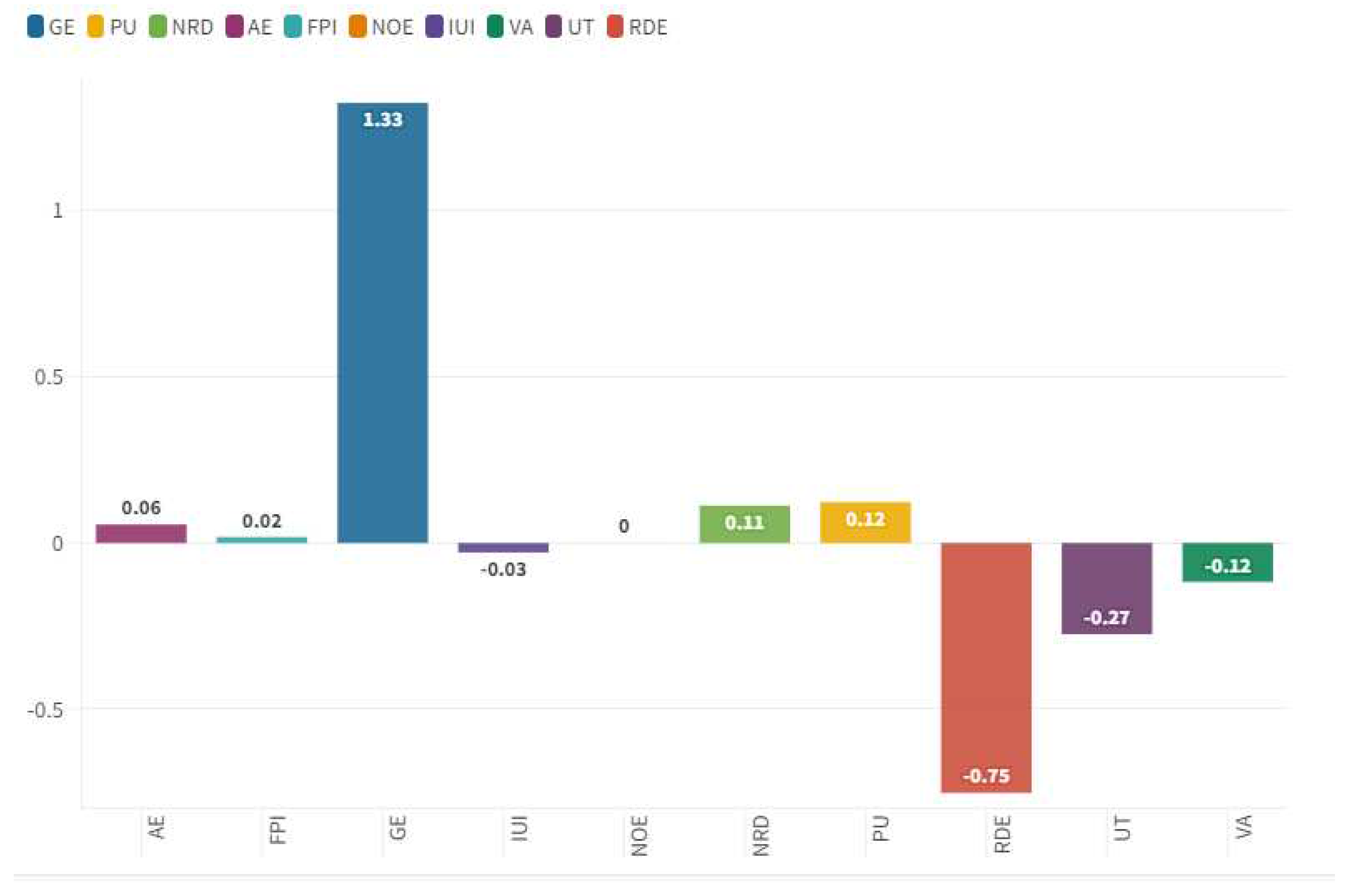
We also found that the value of GDPG rate is negatively associated to:
- IUI: it is a variable that measures the number of individuals who have used the Internet (from any location) in the last 3 months. The Internet can be used via a computer, mobile phone, personal digital assistant, games machine, digital TV etc. There is a negative relationship between IUI and GDPG. The reasoning is that countries that have high levels of economic growth are also countries that have low internet access. In fact, these are African or Asian countries with low per capita incomes that do not have internet coverage such as to allow the entire population to have the benefits of the digital economy. Countries with a high GDPG rate have low levels of digitization. These countries are growing thanks to Foreign Direct Investment-FDI, relocations, low labor costs, and the availability of raw materials useful for industrial production.
- VA: captures perceptions of the extent to which a country’s citizens are able to participate in selecting their government, as well as freedom of expression, freedom of association, and a free media. Standard error indicates the precision of the estimate of governance. Larger values of the standard error indicate less precise estimates. A 90 percent confidence interval for the governance estimate is given by the estimate +/- 1.64 times the standard error. There is a negative relationship between VA and GDPG. This negative relationship is since many countries that have a high GDPG value are countries with low per capita income that do not have the possibility to exercise democratic and civil freedoms. In fact, these are countries in which a profound democratic culture is not to be found and which experience questionable political regimes from a strictly democratic point of view. Conversely, Western countries in which the value of VA is high have low levels of GDPG rate. The negative relationship between VA and GDPG confirms that economic growth tends to be more marked for those countries that have low per capita incomes and are therefore in the early stages of economic, social, and institutional development.
- UT: refers to the share of the labor force that is out of work but available for and looking for work. There is a negative relationship between the UT model and the GDPG rate model. This relationship is since the growth of the GDP tends to generate a growth also in employment and therefore a reduction in unemployment. Increasing the level of economic activity allows countries to increase employment in both the public and private sectors with a significant reduction in unemployment. Countries that grow the most in terms of GDP are also those that have the largest share of agriculture and manufacturing as percentage of value added. The employment in agricultural and manufacture sectors do not require a high-skilled workforce. Therefore, the increase in the offer of labor in agriculture, construction and industry has an immediate impact in reducing unemployment even for non-educated workers.
- RDE: is a variable that measures the gross domestic expenditure on research and development (R&D), expressed as a percentage of GDP. They include both capital and current spending across the four major sectors: business, government, higher education, and private non-profits. R&D covers basic research, applied research and experimental development. There is a negative relationship between RDE and GDPG. This relationship is since countries with higher GDPG rates also have lower investment in research and development. Countries with a high GDPG rate are not countries with a high per capita income, with advanced economies from the point of view of services and therefore do not need to invest in R&D. Conversely, countries with a low GDPG rate and a high level of per capita income must invest in research and development to maintain the competitiveness of their businesses and their economy.
The econometric analysis shows that the value of GDPG rate increases in connection with relevant social and government variables i.e. GE and UT. However, the GDPG rate value is also negatively associated with environmental issues as demonstrated by NOE and NRD. It follows that while the process of economic growth is certainly compatible with governance and social issues, it is not equally compatible with environmental ones. In fact, the triggering of economic growth requires the consumption of large quantities of energy which have negative impacts on the environment. However, the positive relationship between economic growth and pollution is not an inescapable necessity. It is probable that in the future new forms of clean and sustainable energy could generate positive effects in terms of compatibility of GDP growth with the environment.
4. Clusterization with the k-Means Algorithm Optimized with the Elbow Method
Below is a clusterization with K-means algorithm optimized with the Elbow method. However, before applying the Elbow method we tried to apply the Silhouette coefficient method. The Silhouette coefficient is an index that varies from -1 to +1 and that can be attributed either to the clusters either to the individual elements within the clusters. The number of optimal clusters is the one that has a higher value, or close to 1. However, by applying the method of the Silhouette coefficient to the historical series of the countries for GDP Growth, the result was unsatisfactory. In fact, we found the presence of only two clusters in a dataset of 193 countries of which one made up of most of the countries and the other composed of a sparse minority of countries. Therefore, we first decided to eliminate the outliers from the distribution and later to replace the Silhouette coefficient with the Elbow method. In fact, the k-Means algorithm is a non-supervised algorithm and requires that the operator will arrange the optimal number of k such as to determine the optimization of the structure in cluster. Therefore, following the elimination of the outliers, the Elbow method was chosen obtaining a structure of three balanced clusters in terms of statistical numerosity. From a strictly quantitative point of view or considering the median value of the GDP Growth for individual countries it appears that the following order: C1 = 5.3> C3 = 4.8> C2 = 4.12.
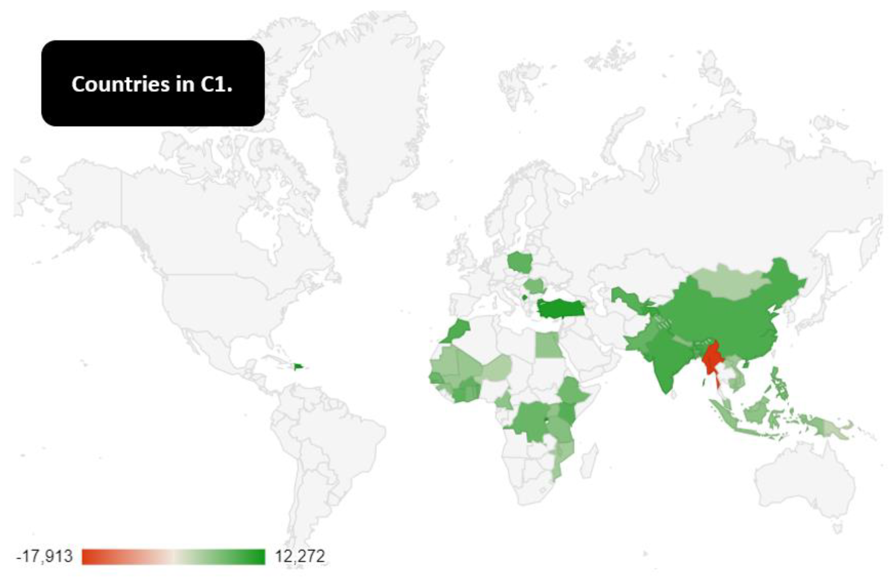
- Cluster 1: Armenia, Bangladesh, Benin, Bhutan, Burkina Faso, Cambodia, Cameroon, China, Congo, Dem. Rep., Cote d’Ivoire, Dominican Republic, Egypt, Arab Rep., Ethiopia, Ghana, Guinea, India, Indonesia, Kenya, Kosovo, Lao PDR, Malawi, Malaysia, Mali, Malta, Mauritania, Mongolia, Morocco, Mozambique, Myanmar, Nepal, Niger, Pakistan, Papua New Guinea, Philippines, Poland, Romania, Rwanda, Senegal, Tajikistan, Tanzania, Togo, Turkey, Tuvalu, Uganda, Uzbekistan, Vietnam. C1 is the cluster with the highest median value in terms of GDPG rate with an amount of 5.3%. However, within this cluster there are countries that in 2021 have had a much higher GDPG rate. The top ten of the C1 countries for the value of the GDPG rate in 2021 consists of Dominican Republic with 12.27%, Turkey with a value of 11.35%, Rwanda with 10.88%, Kosovo with 10.75%, Malta with 10.30%, Tajikistan with 9.20, India 8.68%, China with 8.11%, Morocco with 7.93%, Kenya with 7.52%. In the last place in the ranking of Cluster 1 countries there is Myanmar with a value of -17.91%. The quantitative trend of the GDPG rate of the Myanmar has a fluctuating trend. Between 2011 and 2020 the average GDPG rate in Myanmar was equal to a value of 6.60%. However, between 2020 and 2021 the GDPG rate went from 3.17% up to -17.91%. This reduction in Myanmar GDPG rate between 2020 and 2021 is due to the coup d’état in the country that laid President Aung San Suu Kyi and replaced the democratic government with a military dictatorship. This coup d’état cost about 21.08% of GDP between 2020 and 2021 to the country. C1 countries are all non -European countries except for Romania, Poland, and Kosovo. In the C1 it is possible to identify the presence of many of the economies that will certainly be the protagonists of the economy of the future such as China, India, and Turkey, Indonesia, Egypt, and Nigeria. The fact that these countries have a very high GDPG rate is due to a set of economic and institutional conditions. In fact, the countries that have low per capita incomes tend to grow quickly if they can attract Foreign Direct Investment-FDI. However, there are also favorable political conditions such as political stability, and the lack of terrorism or state strokes. Most C1 countries are Asian and African countries. However, there are doubts that the growth rate of these countries can continue to grow in the future. For example, in the case of China it is likely that the choice of an anti-western and isolationist turning point can lead to a reduction in the value of the GDPG rate which is very connected to the development of FDI and international supply chain. Similar considerations hold also for the other C1 countries that seem to be characterized by a basic political instability that could generate a return to low growth conditions and poverty preceding the development of commercial integration and globalization. It follows that the C1 countries are certainly the best in terms of GDPG rate. However, there are many political, economic, and institutional risks that could reduce the value of their economic growth in the future. Furthermore, it should be considered that the value of GDPG rate in C1 countries could be reduced by phenomena connected to mass immigration and the adverse effects of the climate change.
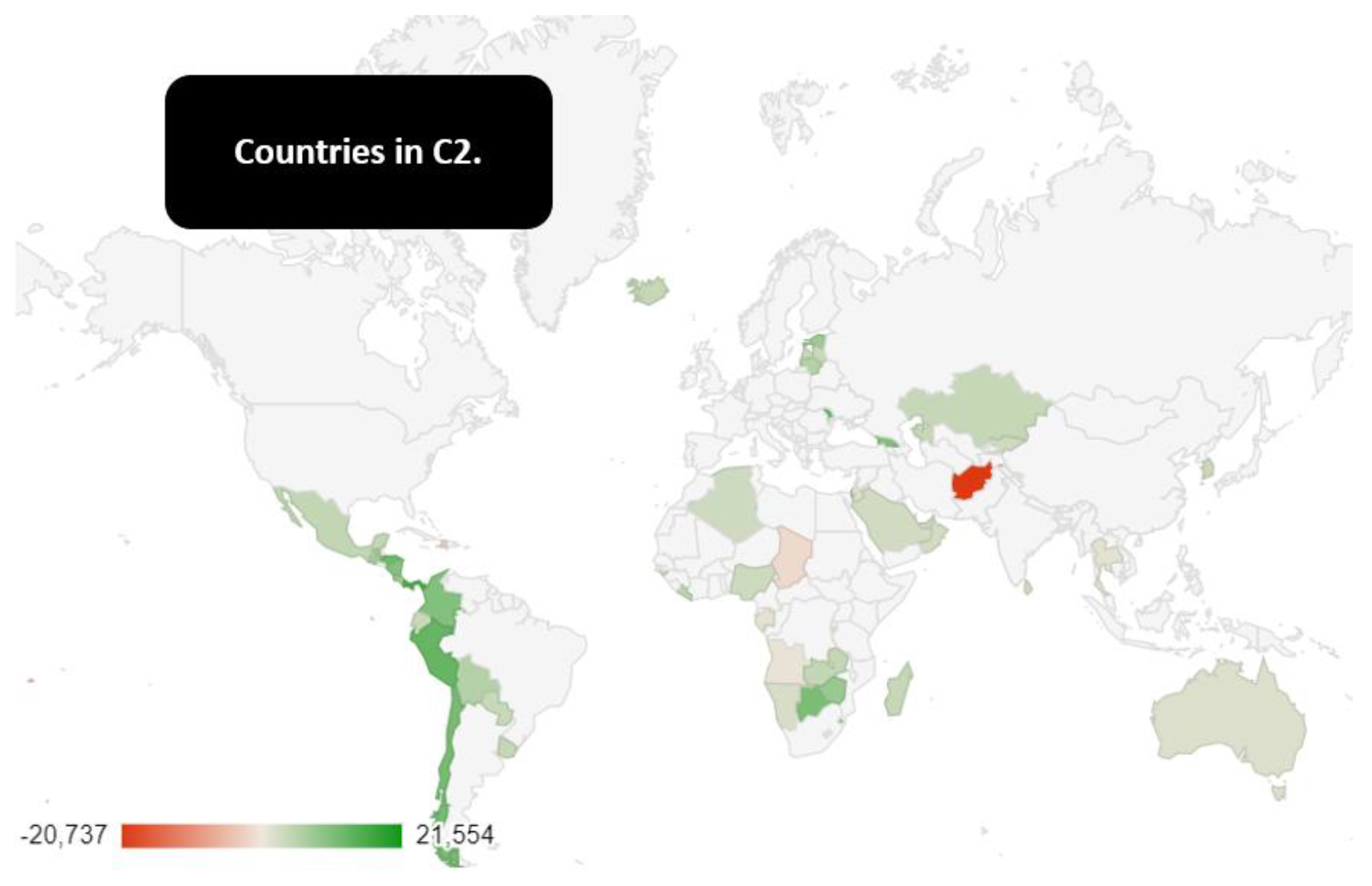
- Cluster 2: Afghanistan, Algeria, Angola, Australia, Bahrain, Bolivia, Botswana, Burundi, Chad, Chile, Colombia, Comoros, Costa Rica, Ecuador, Estonia, Eswatini, Fiji, Gabon, Georgia, Guatemala, Guinea-Bissau, Haiti, Honduras, Hong Kong, Iceland, Israel, Jordan, Kazakhstan, Kiribati, Korea, Rep., Kyrgyz Republic, Latvia, Lesotho, Liberia, Lithuania, Madagascar, Mauritius, Mexico, Moldova, Monaco, Namibia, New Zealand, Nicaragua, Nigeria, Oman, Panama, Paraguay, Peru, Qatar, Sao Tome and Principe, Saudi Arabia, Seychelles, Singapore, Solomon Islands, Sri Lanka, Thailand, Tonga, United Arab Emirates, Uruguay, West Bank and Gaza, Zambia, Zimbabwe. The C2 is the last cluster in terms of median value of the GDPG rate among the three identified clusters. The top ten of the countries by the value of the GDPG rate in 2021 consists of Monaco with a value of 21.55%, followed by Panama with a value of 15.34%, from Moldova with a value of 13.94%, from Peru with an amount of 13.35%, Honduras with a value of 12.53%, Chile with 11.67%, Botswana 11.37%, Colombia with 10.68%, Georgia with 10.47%, Nicaragua with 10.34%.
Figure 2.
Countries in C1.
Inside C2 it is possible to find Afghanistan a country that had a very positive GDPG rate trend until 2019. However, GDPG rate for Afghanistan has worsened both in 2020 with -2.35% and in 2021 with -20.73%. The reduction of the GDPG rate of Afghanistan is closely connected to the conclusion of the NATO-US occupation in the country and the return of the Taliban. The return of the Taliban has thrown the country into a condition of economic and political crisis, as well as a new international isolation, with a reduction in the civil rights and freedom and the life expectancy of the population. The C2 is made up of medium-low-income countries with some exceptions such as Monaco, Singapore, Israel, Hong Kong, Iceland, South Korea, Australia. From a geographical point of view, the C2 has a very low degree of homogeneity, being made up of countries that are part of all continents. These are countries that have not prospectively a very high growth capacity in terms of GDP and that appear very stable within the international system. However, the income of these countries tends to grow. Probably the C2 countries that will grow more in terms of GDPG rate are Mexico, Nigeria, and South Korea i.e. three countries that are part of the Next Eleven-N11 group. It is probable that these countries continue in their path of economic growth without becoming particularly relevant to an individual level in terms of the production of GDP.
Figure 3.
Countries in C2.
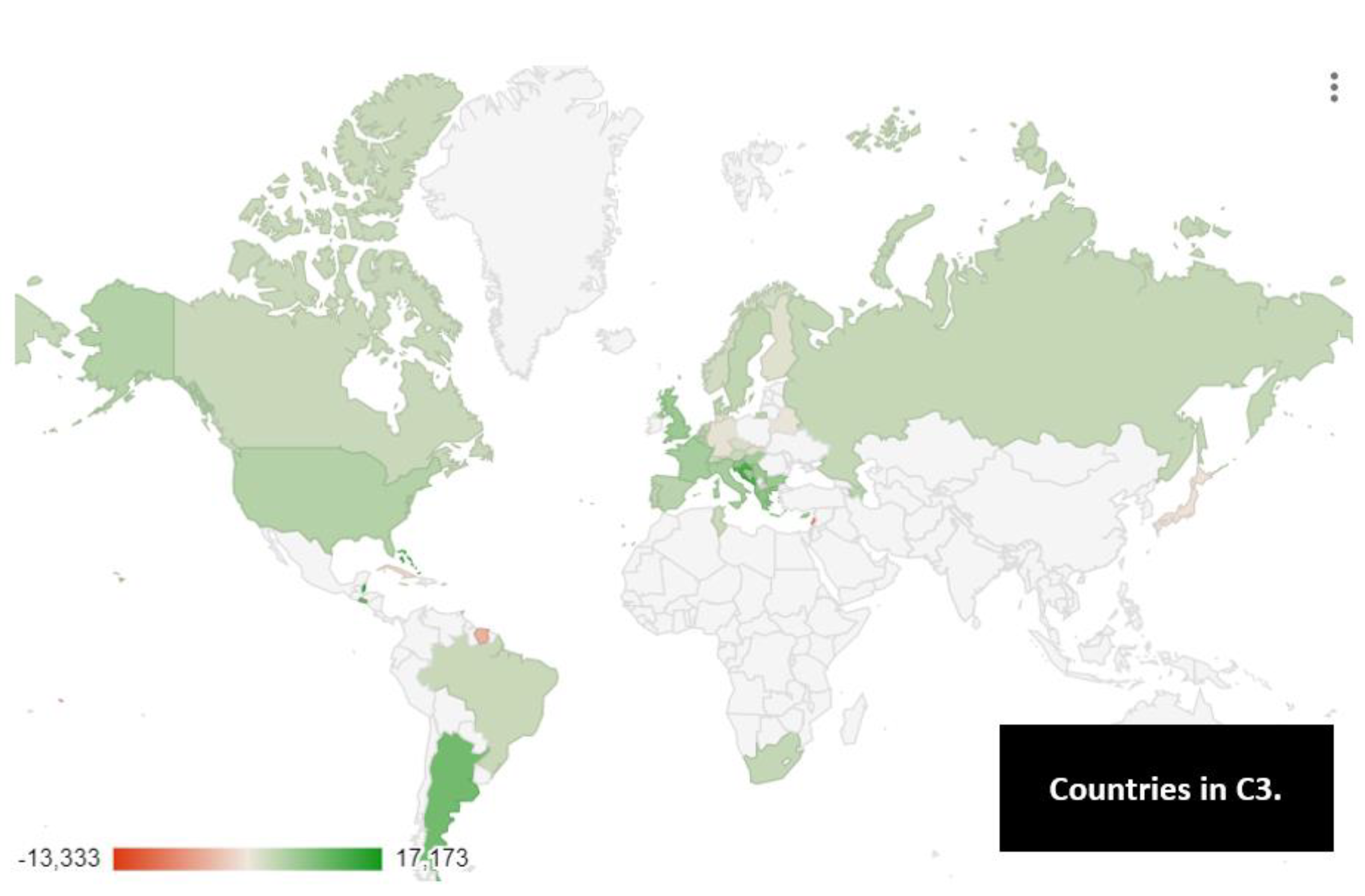
- Cluster 3: Albania, Andorra, Antigua and Barbuda, Argentina, Aruba, Austria, Azerbaijan, The Bahamas, Barbados, Belarus, Belgium, Belize, Bermuda, Bosnia and Herzegovina, Brazil, Brunei Darussalam, Bulgaria, Cabo Verde, Canada, Cayman Islands, Croatia, Cuba, Curacao, Cyprus, Czechia, Denmark, Dominica, El Salvador, Finland, France, French Polynesia, Germany, Greece, Grenada, Guam, Hungary, Italy, Jamaica, Japan, Lebanon, Luxembourg, Marshall Islands Micronesia Fed. Sts., Montenegro, Netherlands, North Macedonia, Norway, Palau, Portugal, Puerto Rico, Russian Federation, Samoa, Serbia, Slovak Republic, Slovenia, South Africa, Spain, St. Kitts and Nevis, St. Lucia, St. Vincent and the Grenadines, Suriname, Sweden, Switzerland, Trinidad and Tobago, Tunisia, United Kingdom, United States, Vanuatu. The C3 is the second cluster for the value of the GDPG rate with a median value equal to an amount of C3 = 4.8. The top ten of the GDPG rate countries consists of Belize with a value of 15.23%, The Bahamas with 13.72%, Croatia with 13.07%, Montenegro with 12.43%, St. Lucia with 12.23%, Argentina with 10.40%, El Salvador with 10.28%, Andorra with 8.95%, Albania with 8.52%, Greece with 8.43%. The C3 consists of a set of countries that essentially coincide with the western world, namely Europe, North America, Japan with the addition of some Latin America countries and South Africa. Russia is present in the C3. The GDPG rate of Russia was positive from 2011 to 2014, with a negative decline in 2015. Subsequently between 2016 and 2019 the value of the GDPG rate grew, and then decreased again in 2020 and grow in 2021 up to a value of 4.75%.
Figure 4.
GDPG rate of some high-income countries in C3 with the indication of the Rebound effect i.e. the increase of GDPG rate in the post Covid-19 Crisis with a value greater than the previous average.
Figure 4.
GDPG rate of some high-income countries in C3 with the indication of the Rebound effect i.e. the increase of GDPG rate in the post Covid-19 Crisis with a value greater than the previous average.
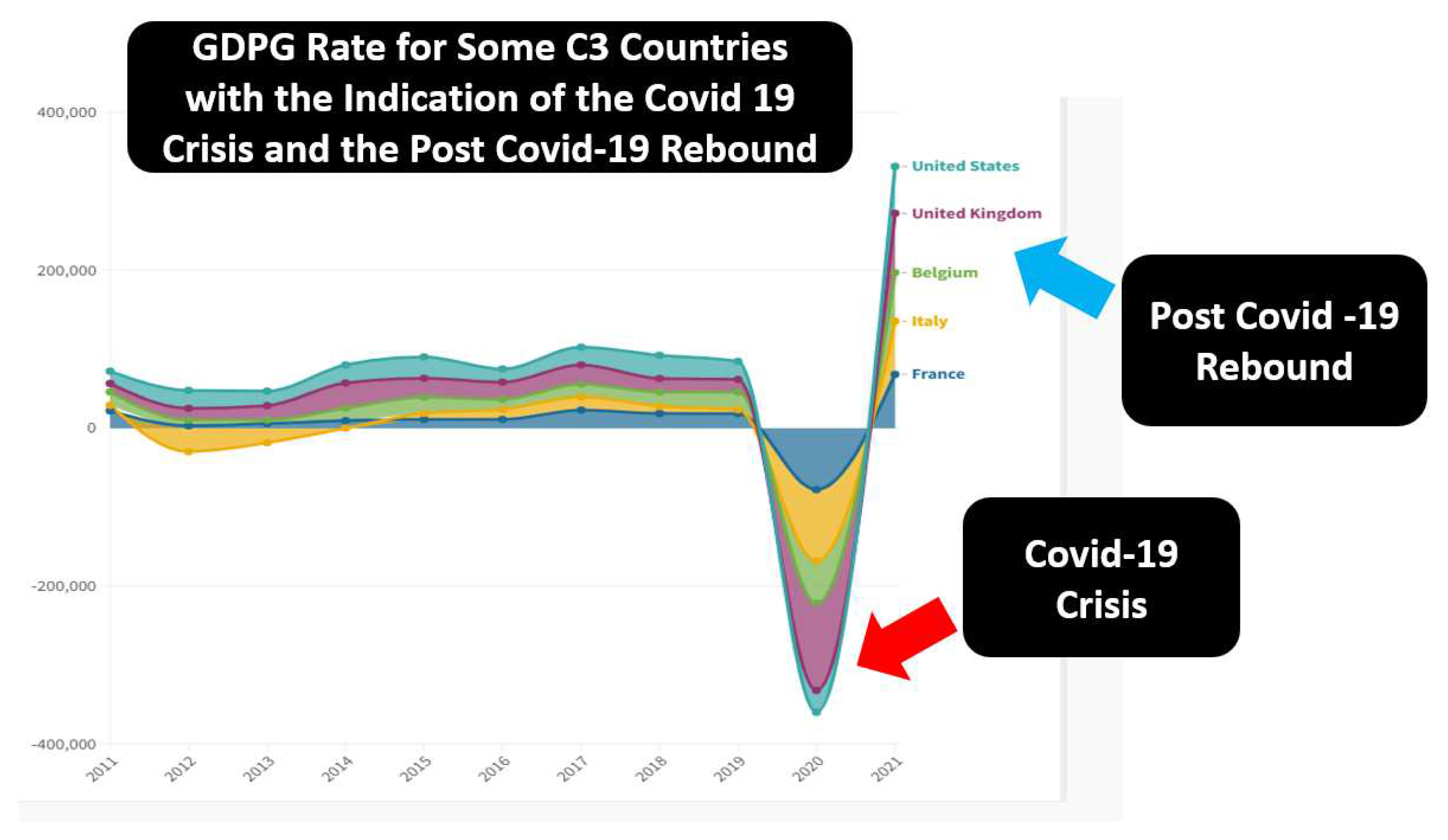
On average between 2011 and 2021 the average value of the GDPG rate of Russia was equal to an amount of 1.63%. However, it is very likely that the choice of Russia to attack Ukraine has a negative effect in terms of GDPG rate. In fact, the penalties that have been imposed on Russia will certainly have negative impacts in GDPG rate terms. It should be considered that GDPG Rates in 2021 for C3 countries are very high, especially for the C3 countries that have a medium-high pro-capita income value. Generally, countries with high-medium income, as that in C3, have a low GDPG Rate. If we look at the trend of GDP in France, Italy, Belgium, UK, and USA we can see that the value of the GDPG rate has decreased between 2019 and 2020 and then grew between 2020 and 2021. This condition is due the reduction of GDP in relation to Covid in 2019 and then grow between 2020 and 2021 with a “rebound” effect that brought the GDPG Rate to a much higher level than the previous average. The fact that a rebound effect occurred following the crisis from Covid 19 is since during the Covid-19 crisis it was not lost production capacity. In fact, the closings of companies, the limitations to travel, the rupture of the supply chains imposed by governments following the Covid 19 were arranged for public health reasons. However, potential production capacity has remained essentially intact at national level. Therefore, the end of the lockdown allowed the resumption of productivity with a significant growth in terms of GDP. This GDP growth in post lockdown has generated a rebound effect.
Figure 5.
Countries in C3.
5. Machine Learning and Predictions for the Estimation of the Future Value of GDPG Rate
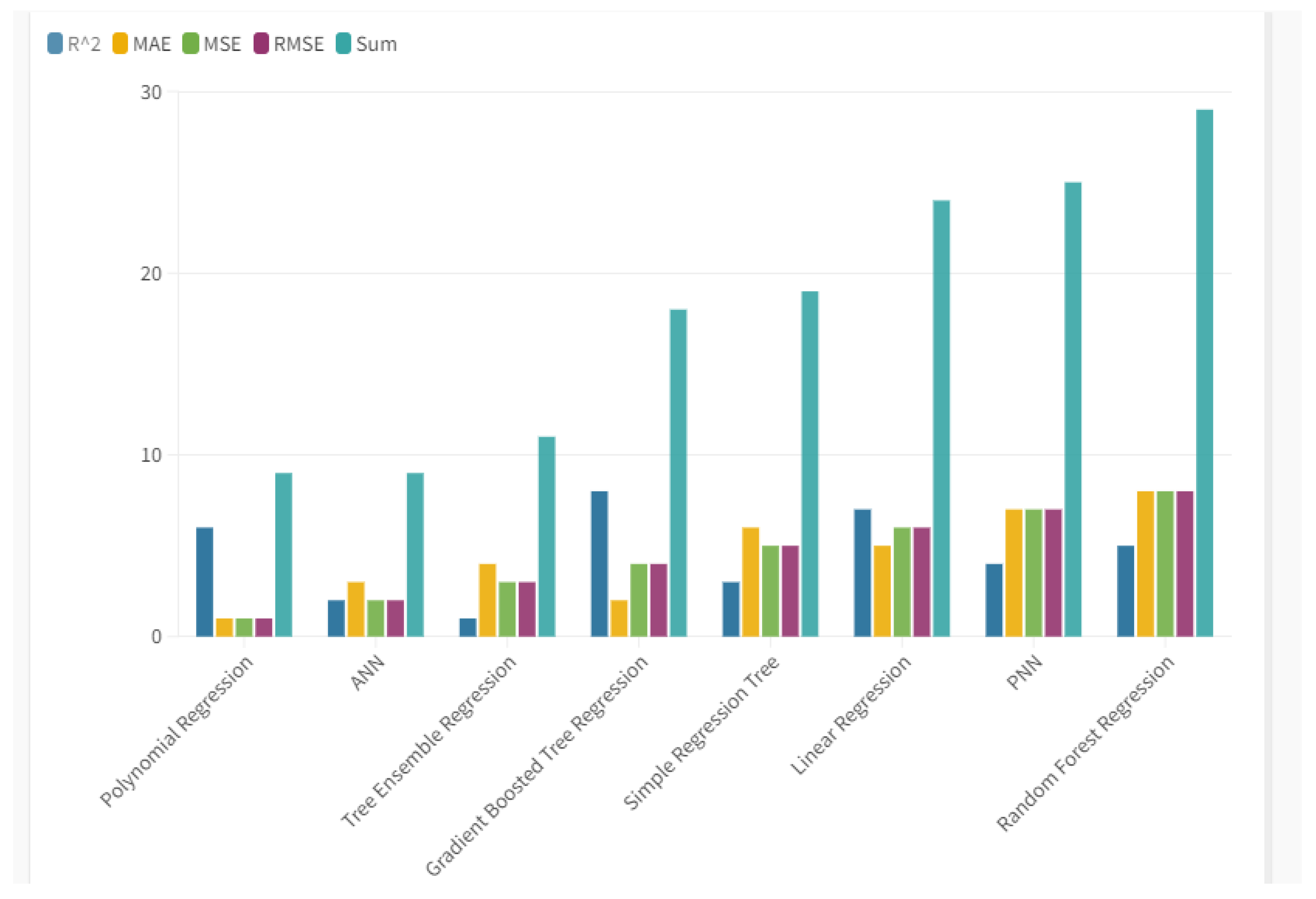
Below is a comparison between eight different Machine Learning algorithms for the prediction of the future value of the GDPG Rate. The algorithms are evaluated based on the maximization of the R-Squared and on the minimization of statistical errors Mean Average Error-MAE, Mean Squared Error-MSE, Root Mean Squared Error-RMSE. The algorithms were trained using 70% of the data while the remaining 30% was used to carry out the actual prediction. Based on the analysis, the following system of algorithms in terms of performance or:
- Polynomial Regression and Ann-Artificial Neural Network with a payoff value of 9;
- Tree regression ensemble with a payoff value of 11;
- Gradient Boosted Tree Regression with a payoff value of 18;
- Simple Regression Tree with a payoff value of 19;
- Linear Regression with a payoff value of 24;
- PNN-Probabilistic Neural Network with a payoff value of 25;
- Random Forest Regression with a payoff value of 29.
Figure 6.
The Ranking of Algorithms Based on R-squared, MAE, MSE, RMSE.
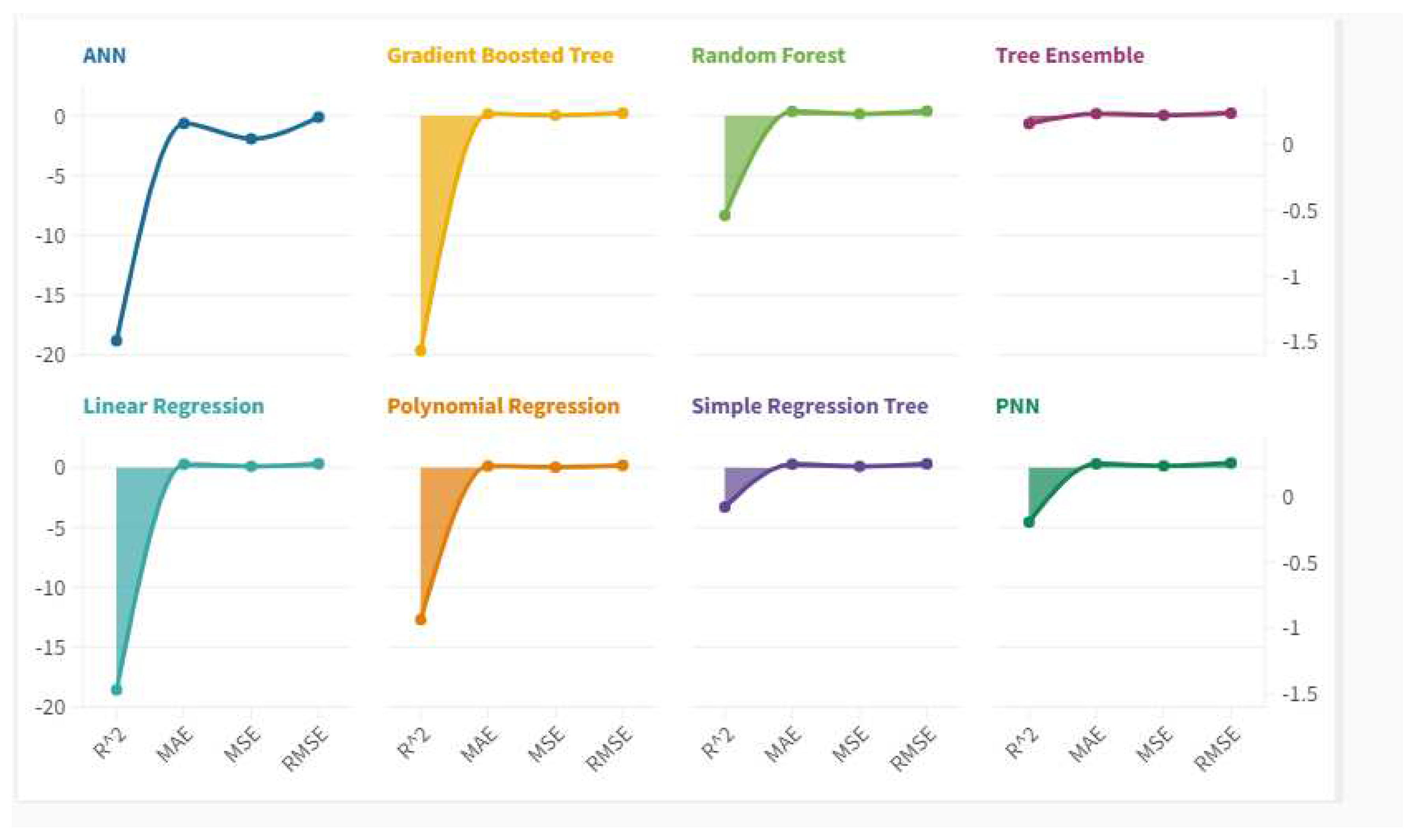
It therefore appears that in the first place in performative terms there are two algorithms or Ann-artificial neural Network and Polynomial Regression. However, following an analysis it appears that the Polynomial regression value is more efficient than ANN in terms of MAE, MSE and RMSE. Therefore, we choose the Polynomial Regression algorithm as Best Predictor.
Figure 7.
Statistical results for each algorithm based on R-squared, MAE, MSE, RMSE.
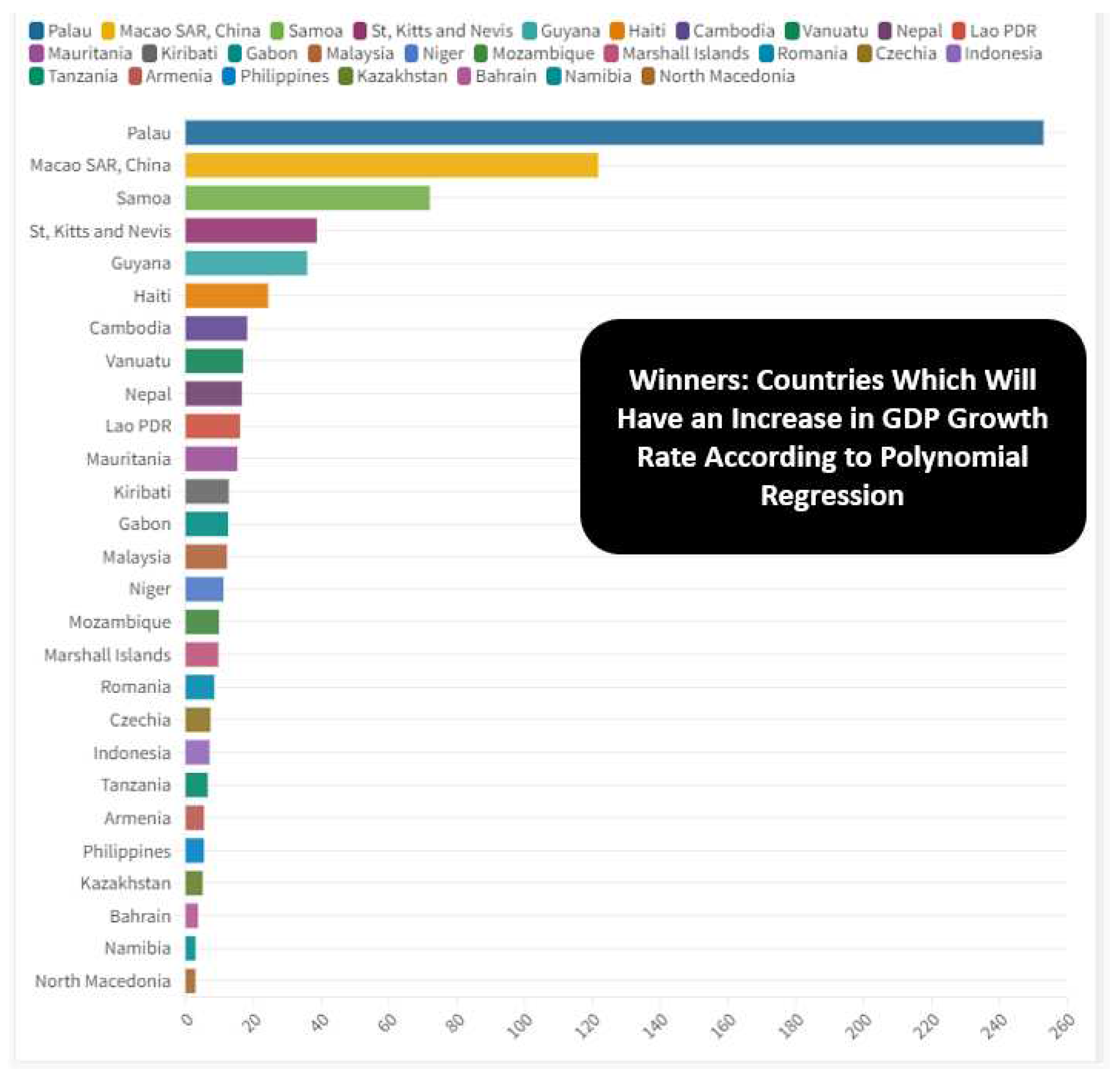
Through the application of the Polynomial Regression algorithm, it is possible to identify a future trend of the value of GDPG rate. On average, the value of GDPG rate is expected to grow for the countries analyzed for an average value equal to a value of 2.88%. However, there are countries that can be considered as Losers, or the countries for which a reduction in the value of GDPG rate is predicted, and the countries that are winners, or the countries for which a growth in the GDPG value is predicted installments. The top ten of the winners’ countries is composed as below or: Palau with +252.96%, Macao with 121.68%, Samoa with 71.99%, St. Kitts and Nevis with a value of 38.7%, Guyana with 35.87%, Haiti with 24.36%, Cambodia with 18.16%, Vanuatu with 16.94%, Nepal with 16.61%, Lao with 16.07%. However, there are also the Losers countries or the countries for which a reduction in the value of the GDPG Rate is predicted. The top ten of the losers in terms of GDPG rate are: Central African Republic with -50.3%, Belize with -25.87%, Croatia with -23.85%, Moldova with -21.03%, Guinea Equatorial with -20.22%, Botswana with -19.58%, Peru with -18.74%, Cote D’Ivoire with -18.44%; Albania with -16.41%, Luxembourg with -14.96%.
Figure 8.
Losers: Countries which Will Have a Reduction in GDP Growth Rate According to Polynomial Regression.
Figure 8.
Losers: Countries which Will Have a Reduction in GDP Growth Rate According to Polynomial Regression.
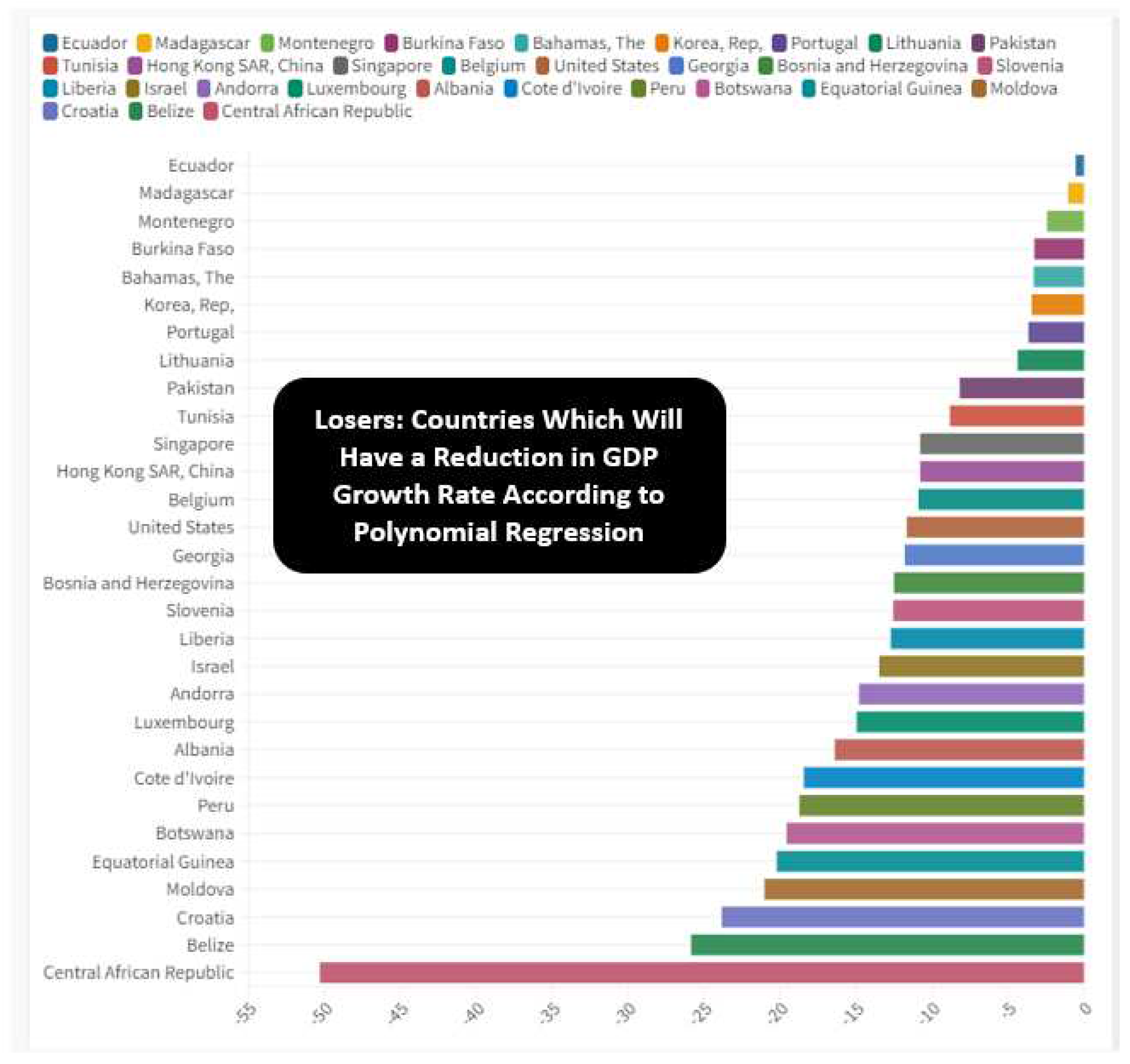
However, it is necessary to consider whether the predictions of the Polynomial Regression algorithm really make sense of what the short-term macro-economic trend can be. We therefore consider some countries for which the prediction is not efficient. First, there are Romania and the Czech Republic for which the algorithm predicts respectively a GDPG rate in 8.48% and 7.35%. However, we can see that these values are very high compared to the average trend of the historical series of both Romania and the Czech Republic. In fact, the average of GDPG rate for Romania in the period between 2011 and 2021 was equal to an amount of 3.30%, while for the Czech Republic it was 1.87%. Similarly, it appears that within the countries that are losers there are countries for which the prediction is not very credible such as, for example, in the case of Portugal for which is predicted a GDPG rate reduction of -3.66 %, Hong Kong with -10.78%, Singapore with -10.78, Belgium -10.9%, United States with -11.67%, Israel with -13.48%, Luxembourg with -14.96%, Albania -16.41%. For these countries there is certainly an incorrect prediction. The chances that Singapore’s economy lose 10.78% of GDP and that the US lose 11.67% and Israel’s GDP with -13.48% are practically close to zero.
Figure 9.
Winners: Countries Which Will Have an Increase in GDP Growth Rate According to Polynomial Regression.
Figure 9.
Winners: Countries Which Will Have an Increase in GDP Growth Rate According to Polynomial Regression.
However, should we ask ourselves why the algorithm produced such wrong predictions absolutely without a sense from an economic point of view? The motivation consists in the fact that Covid-19 significantly reduced the GDPG rate between 2019 and 2020 and later between 2020 and 2021 the GDPG Rate has grown significantly with a very high rebound effect. Since this trend can be found in all dataset countries, then it appears that in any case there is a linearity. It follows that in fact the algorithm makes predictions quite misaligned compared to the historical series due to the difficulty of “normalizing” the black swan produced by Covid 19 and the subsequent rebound effect between 2020 and 2021. However, the algorithm is efficient in terms of quantitative evaluation in terms of minimizing statistical errors and maximization of the R-Squared. However, this efficiency detected on a quantitative level does not have sufficient significance on a qualitative level. This means that the Polynomial Regression is the best predictive algorithm based on a statistical analysis. But the qualitative significance of the prediction is not acceptable on an economic point of view.
6. Conclusions
In the following article we highlighted the relationship between GDPG and some variables of the ESG model. The econometric analysis has shown that the value of GDPG grows together with the S variables of the ESG model. The relationship between the G component of the ESG model and GDPG is controversial as GDPG is positively associated with GE and negatively associated with VA. On the contrary, the relationship between the E component of the ESG model and GDPG is negative as GDPG i.e., GDP grows with NOE and NRD. From the point of view of clusterization, it appears that countries that have lowest per-capita income grow more in terms of GDP. The predictive analysis shows a positive trend of GDPG even if the historical series are influenced by the economic manifestation of the Covid 19 pandemic, which has significantly reduced GDP for all countries worldwide. From the point of view of political economy, there is no contradiction between GDPG and ESG except for the E component. In fact, to have access to economic growth, countries need to consume large quantities of energy especially in the case of countries a low per-capita income. It follows that only in the presence of technological innovations that allow to produce cleaner energy will it be possible to create a positive relationship between GDPG and the application of the ESG model, especially for low-income countries.
Funding
The authors received no financial support for the research, authorship, and/or publication of this article.
Data Availability Statement
The data presented in this study are available on request from the corresponding author.
Declaration of Competing Interest
The authors declare that there is no conflict of interests regarding the publication of this manuscript. In addition, the ethical issues, including plagiarism, informed consent, misconduct, data fabrication and/or falsification, double publication.
Software
The authors have used the following software: Gretl for the econometric models, Orange for clusterization and network analysis, and KNIME for machine learning and predictions. They are all free version without licenses.
Acknowledgements
We are grateful to the teaching staff of the LUM University “Giuseppe Degennaro” and to the management of the LUM Enterprise s.r.l. for the constant inspiration to continue our scientific research work undeterred.
Appendix A
| List of Variables | |||
| Acronym | Variables | Description | |
| GDPG | GDP growth | Annual percentage growth rate of GDP at market prices based on constant local currency. Aggregates are based on constant 2015 prices, expressed in U.S. dollars. GDP is the sum of gross value added by all resident producers in the economy plus any product taxes and minus any subsidies not included in the value of the products. It is calculated without making deductions for depreciation of fabricated assets or for depletion and degradation of natural resources. | |
| GE | Government Effectiveness: Estimate | Government Effectiveness captures perceptions of the quality of public services, the quality of the civil service and the degree of its independence from political pressures, the quality of policy formulation and implementation, and the credibility of the government's commitment to such policies. Estimate gives the country's score on the aggregate indicator, in units of a standard normal distribution, i.e. ranging from approximately -2.5 to 2.5. | |
| PU | Prevalence of undernourishment (% of population) | Prevalence of undernourishments is the percentage of the population whose habitual food consumption is insufficient to provide the dietary energy levels that are required to maintain a normal active and healthy life. Data showing as 2.5 may signify a prevalence of undernourishment below 2.5%. | |
| NRD | Adjusted savings: natural resources depletion (% of GNI) | Natural resource depletion is the sum of net forest depletion, energy depletion, and mineral depletion. Net forest depletion is unit resource rents times the excess of roundwood harvest over natural growth. Energy depletion is the ratio of the value of the stock of energy resources to the remaining reserve lifetime (capped at 25 years). It covers coal, crude oil, and natural gas. Mineral depletion is the ratio of the value of the stock of mineral resources to the remaining reserve lifetime (capped at 25 years). It covers tin, gold, lead, zinc, iron, copper, nickel, silver, bauxite, and phosphate. | |
| AE | Access to electricity (% of population) | Access to electricity is the percentage of population with access to electricity. Electrification data are collected from industry, national surveys and international sources. | |
| FPI | Food production index (2014-2016 = 100) | Food production index covers food crops that are considered edible and that contain nutrients. Coffee and tea are excluded because, although edible, they have no nutritive value. | |
| NOE | Nitrous oxide emissions (metric tons of CO2 equivalent per capita) | Nitrous oxide emissions are emissions from agricultural biomass burning, industrial activities, and livestock management. | |
| IUI | Individuals using the Internet (% of population) | Internet users are individuals who have used the Internet (from any location) in the last 3 months. The Internet can be used via a computer, mobile phone, personal digital assistant, games machine, digital TV etc. | |
| VA | Voice and Accountability: Estimate | Voice and accountability captures perceptions of the extent to which a country's citizens are able to participate in selecting their government, as well as freedom of expression, freedom of association, and a free media. | |
| UT | Unemployment, total (% of total labor force) (modeled ILO estimate) | Unemployment refers to the share of the labor force that is without work but available for and seeking employment. | |
| RDE | Research and development expenditure (% of GDP) | Gross domestic expenditures on research and development (R&D), expressed as a percent of GDP. They include both capital and current expenditures in the four main sectors: Business enterprise, Government, Higher education and Private non-profit. R&D covers basic research, applied research, and experimental development. | |
| Random-effects (GLS), using 1930 observations | |||||||||
| Included 193 cross-sectional units | |||||||||
| Time-series length = 10 | |||||||||
| Dependent variable: A24 | |||||||||
| Coefficient | Std. Error | z | p-value | ||||||
| const | −1.02421 | 0.450902 | −2.271 | 0.0231 | ** | ||||
| A2 | 0.0508179 | 0.00509079 | 9.982 | <0.0001 | *** | ||||
| A3 | 0.110081 | 0.0224437 | 4.905 | <0.0001 | *** | ||||
| A21 | 0.0201331 | 0.00391075 | 5.148 | <0.0001 | *** | ||||
| A27 | 1.24176 | 0.115788 | 10.72 | <0.0001 | *** | ||||
| A32 | −0.0336362 | 0.00582231 | −5.777 | <0.0001 | *** | ||||
| A42 | 0.000253546 | 2.95637e-05 | 8.576 | <0.0001 | *** | ||||
| A52 | 0.120953 | 0.0158723 | 7.620 | <0.0001 | *** | ||||
| A58 | −0.725966 | 0.0859671 | −8.445 | <0.0001 | *** | ||||
| A65 | −0.166348 | 0.0276719 | −6.011 | <0.0001 | *** | ||||
| sq_A67 | −0.113606 | 0.0244670 | −4.643 | <0.0001 | *** | ||||
| Mean dependent var | 2.752729 | S.D. dependent var | 7.551392 | ||||||
| Sum squared resid | 73037.27 | S.E. of regression | 6.167677 | ||||||
| Log-likelihood | −6244.830 | Akaike criterion | 12511.66 | ||||||
| Schwarz criterion | 12572.88 | Hannan-Quinn | 12534.18 | ||||||
| rho | −0.044700 | Durbin-Watson | 1.780619 | ||||||
| 'Between' variance = 1.42031 | |||||||||
| 'Within' variance = 34.3654 | |||||||||
| theta used for quasi-demeaning = 0.158831 | |||||||||
| Joint test on named regressors - | |||||||||
| Asymptotic test statistic: Chi-square(10) = 900.44 | |||||||||
| with p-value = 5.12031e-187 | |||||||||
| Breusch-Pagan test - | |||||||||
| Null hypothesis: Variance of the unit-specific error = 0 | |||||||||
| Asymptotic test statistic: Chi-square(1) = 35.4053 | |||||||||
| with p-value = 2.67755e-09 | |||||||||
| Hausman test - | |||||||||
| Null hypothesis: GLS estimates are consistent | |||||||||
| Asymptotic test statistic: Chi-square(10) = 114.382 | |||||||||
| with p-value = 6.95445e-20 | |||||||||
| Pooled OLS, using 1930 observations | |||||||||
| Included 193 cross-sectional units | |||||||||
| Time-series length = 10 | |||||||||
| Dependent variable: A24 | |||||||||
| Coefficient | Std. Error | t-ratio | p-value | ||||||
| const | −0.728472 | 0.426348 | −1.709 | 0.0877 | * | ||||
| A2 | 0.0456025 | 0.00487707 | 9.350 | <0.0001 | *** | ||||
| A3 | 0.104757 | 0.0208237 | 5.031 | <0.0001 | *** | ||||
| A21 | 0.0228313 | 0.00389345 | 5.864 | <0.0001 | *** | ||||
| A27 | 1.25541 | 0.108039 | 11.62 | <0.0001 | *** | ||||
| A32 | −0.0363034 | 0.00541884 | −6.699 | <0.0001 | *** | ||||
| A42 | 0.000256959 | 3.02624e-05 | 8.491 | <0.0001 | *** | ||||
| A52 | 0.107801 | 0.0144890 | 7.440 | <0.0001 | *** | ||||
| A58 | −0.710193 | 0.0788078 | −9.012 | <0.0001 | *** | ||||
| A65 | −0.153762 | 0.0242095 | −6.351 | <0.0001 | *** | ||||
| sq_A67 | −0.109099 | 0.0247975 | −4.400 | <0.0001 | *** | ||||
| Mean dependent var | 2.752729 | S.D. dependent var | 7.551392 | ||||||
| Sum squared resid | 72937.05 | S.E. of regression | 6.165050 | ||||||
| R-squared | 0.336926 | Adjusted R-squared | 0.333471 | ||||||
| F(10, 1919) | 97.50964 | P-value(F) | 2.9e-163 | ||||||
| Log-likelihood | −6243.505 | Akaike criterion | 12509.01 | ||||||
| Schwarz criterion | 12570.23 | Hannan-Quinn | 12531.53 | ||||||
| rho | 0.134672 | Durbin-Watson | 1.481766 | ||||||
| Fixed-effects, using 1930 observations | |||||||||
| Included 193 cross-sectional units | |||||||||
| Time-series length = 10 | |||||||||
| Dependent variable: A24 | |||||||||
| Coefficient | Std. Error | t-ratio | p-value | ||||||
| const | −0.212097 | 0.863193 | −0.2457 | 0.8059 | |||||
| A2 | 0.0701063 | 0.00669856 | 10.47 | <0.0001 | *** | ||||
| A3 | 0.122665 | 0.0358979 | 3.417 | 0.0006 | *** | ||||
| A21 | 0.0106832 | 0.00423368 | 2.523 | 0.0117 | ** | ||||
| A27 | 1.47789 | 0.188431 | 7.843 | <0.0001 | *** | ||||
| A32 | −0.0155919 | 0.00865741 | −1.801 | 0.0719 | * | ||||
| A42 | 0.000239513 | 2.89026e-05 | 8.287 | <0.0001 | *** | ||||
| A52 | 0.141313 | 0.0312518 | 4.522 | <0.0001 | *** | ||||
| A58 | −0.821873 | 0.150486 | −5.461 | <0.0001 | *** | ||||
| A65 | −0.504057 | 0.0933865 | −5.398 | <0.0001 | *** | ||||
| sq_A67 | −0.128323 | 0.0247580 | −5.183 | <0.0001 | *** | ||||
| Mean dependent var | 2.752729 | S.D. dependent var | 7.551392 | ||||||
| Sum squared resid | 59349.05 | S.E. of regression | 5.862201 | ||||||
| LSDV R-squared | 0.460455 | Within R-squared | 0.284820 | ||||||
| LSDV F(202, 1727) | 7.296266 | P-value(F) | 1.2e-127 | ||||||
| Log-likelihood | −6044.560 | Akaike criterion | 12495.12 | ||||||
| Schwarz criterion | 13624.87 | Hannan-Quinn | 12910.69 | ||||||
| rho | −0.044700 | Durbin-Watson | 1.780619 | ||||||
| Joint test on named regressors - | |||||||||
| Test statistic: F(10, 1727) = 68.7778 | |||||||||
| with p-value = P(F(10, 1727) > 68.7778) = 3.02506e-118 | |||||||||
| Test for differing group intercepts - | |||||||||
| Null hypothesis: The groups have a common intercept | |||||||||
| Test statistic: F(192, 1727) = 2.05936 | |||||||||
| with p-value = P(F(192, 1727) > 2.05936) = 6.03502e-14 | |||||||||
References
- Costantiello e A. Leogrande, «The Determinants of CO2 Emissions in the Context of ESG Models at World Level,» 2023.
- L. Laureti, A. Massaro, A. Costantiello e A. Leogrande, «The Impact of Renewable Electricity Output on Sustainability in the Context of Circular Economy: A Global Perspective,» Sustainability, vol. 3, n. 2160, p. 15, 2023.
- L. Laureti, A. Costantiello e A. Leogrande, «The Role of Renewable Energy Consumption in Promoting Sustainability and Circular Economy. A Data-Driven Analysis.,» 2022.
- Costantiello e A. Leogrande, «The Role of Political Stability in the Context of ESG Models at World Level,» University Library of Munich, Germany, 2023.
- Costantiello e A. Leogrande, «The Impact of Voice and Accountability in the ESG Framework in a Global Perspective,» SSRN , n. 4398483, 2023.
- Costantiello e A. Leogrande, «The Regulatory Quality and ESG Model at World Level,» 2023.
- Leogrande, «The Rule of Law in the ESG Framework in the World Economy,» University Library of Munich, Germany, n. 116293, 2023.
- L. Laureti, A. Costantiello e A. Leogrande, «The Role of Government Effectiveness in the Light of ESG Data at Global Level,» University Library of Munich, Germany, n. 115998, 2023.
- L. Laureti, A. Costantiello e A. Leogrande, «The Fight Against Corruption at Global Level. A Metric Approach,» 2023.
- Costantiello e A. Leogrande, «The Ease of Doing Business in the ESG Framework at World Level,» 2023.
- Costantiello e A. Leogrande, «The Impact of Research and Development Expenditures on ESG Model in the Global Economy,» 2023.
- G. Cohen, «ESG risks and corporate survival.,» Environment Systems and Decisions, pp. 1-6, 2022.
- Morgenstern, G. Coqueret e J. Kelly, «International market exposure to sovereign ESG,» Journal of Sustainable Finance & Investment, pp. 1-20, 2022.
- P. Naomi e I. Akbar, «Beyond sustainability: Empirical evidence from OECD countries on the connection among natural resources, ESG performances, and economic development,» Economics & Sociology, vol. 14, n. 4, pp. 89-106, 2021.
- W. Puttachai, R. Phadkantha e W. Yamaka, «The threshold effects of ESG performance on the energy transitions: A country-level data,» Energy Reports, vol. 8, pp. 234-241, 2022. [CrossRef]
- T. H. Ng, C. T. Lye, K. H. Chan, Y. Z. Lim e Y. S. Lim, «Sustainability in Asia: The roles of financial development in environmental, social and governance (ESG) performance,» Social Indicators Research, vol. 150, pp. 17-44, 2020.
- H. Al Amosh e S. F. Khatib, «ESG performance in the time of COVID-19 pandemic: cross-country evidence,» Environmental Science and Pollution Research, pp. 1-16, 2023. [CrossRef]
- V. Cherkasova e I. Nenuzhenko, «Investment in ESG Projects and Corporate Performance of Multinational Companies,» Journal of Economic Integration, vol. 37, n. 1, pp. 54-92, 2022. [CrossRef]
- S. H. Ho, R. Oueghlissi e R. El Ferktaji, «The dynamic causality between ESG and economic growth: Evidence from panel causality analysis,» 2019.
- Ye, X. Song e Y. Liang, «Corporate sustainability performance, stock returns, and ESG indicators: fresh insights from EU member states,» Environmental Science and Pollution Research, vol. 58, n. 87680-87691, p. 29, 2022.
- G. Ferri e A. Leogrande, «Was the Crisis Due to a Shift from Stakeholder to Shareholder Finance? Surveying the Debate. No. 1576.,» Euricse (European Research Institute on Cooperative and Social Enterprises), n. 176, 2015.
- G. Ferri e A. Leogrande, «Stakeholder Management, Cooperatives, and Selfish-Individualism,» Journal for Markets and Ethics, vol. 9, n. 2, pp. 61-75, 2021.
- G. Ferri e A. Leogrande, «The Founding Role of Cooperative Banking Within the European Variety of Capitalism,» in Contemporary Trends in European Cooperative Banking: Sustainability, Governance, Digital Transformation, and Health Crisis Response , vol. Springer International Publishing., Cham , Springer International Publishing., 2022, pp. 29-54.
- G. Birindelli, S. Dell’Atti, A. P. Iannuzzi e M. Savioli, «Composition and activity of the board of directors: Impact on ESG performance in the banking system,» Sustainability, vol. 12, n. 4699, p. 10, 2018.
- Buallay, «Is sustainability reporting (ESG) associated with performance? Evidence from the European banking sector,» Management of Environmental Quality: An International Journal, vol. 30, n. 1, pp. 98-115, 2019. [CrossRef]
- M. M. Miralles-Quirós, J. L. Miralles-Quirós e J. Redondo Hernández, «ESG performance and shareholder value creation in the banking industry: International differences,» Sustainability, vol. 5, n. 1404, p. 11, 2019. [CrossRef]
- H. Maama, «Institutional environment and environmental, social and governance accounting among banks in West Africa,» Meditari Accountancy Research, vol. 6, n. 1314-1336, p. 29, 2021. [CrossRef]
- X. Zhou, B. Caldecott, E. Harnett e K. Schumacher, «The effect of firm-level ESG practices on macroeconomic performance,» University of Oxford| Working Paper, vol. 20, n. 03, 2020.
- Breedt, S. Ciliberti, S. Gualdi e P. Seager, «Is ESG an equity factor or just an investment guide?,» SSRN, 2019. [CrossRef]
- M. Alandejani e H. Al-Shaer, «Macro Uncertainty Impacts on ESG Performance and Carbon Emission Reduction Targets,» Sustainability, vol. 5, n. 4249, p. 15, 2023. [CrossRef]
- H. Al Amosh e S. F. Khatib, «ESG performance in the time of COVID-19 pandemic: cross-country evidence,» Environmental Science and Pollution Research, pp. 1-16, 2023. [CrossRef]
Disclaimer/Publisher’s Note: The statements, opinions and data contained in all publications are solely those of the individual author(s) and contributor(s) and not of MDPI and/or the editor(s). MDPI and/or the editor(s) disclaim responsibility for any injury to people or property resulting from any ideas, methods, instructions or products referred to in the content. |
© 2023 by the authors. Licensee MDPI, Basel, Switzerland. This article is an open access article distributed under the terms and conditions of the Creative Commons Attribution (CC BY) license (http://creativecommons.org/licenses/by/4.0/).
Copyright: This open access article is published under a Creative Commons CC BY 4.0 license, which permit the free download, distribution, and reuse, provided that the author and preprint are cited in any reuse.


