
Submitted:
03 May 2023
Posted:
04 May 2023
You are already at the latest version
Abstract
Through the arrow decomposition of the Mueller matrix, respective sets of sixteen independent polarimetric images of biological tissues are obtained for enpolarizing, retarding and depolariz-ing descriptors. In addition to the mean intensity coefficient and the three indices of polarimetric purity, the absolute values and Poincaré orientations of diattenuation, polarizance, entrance re-tardance and exit retardance vectors are considered. In this work we use for the first time this set of polarimetric observables for the visualization of biological structures, both of animal and vege-tal origin. Results show images with enhanced visualization derived from the spatial variation of such significant polarimetric properties. The experimental results are discussed, showing the suit-ability of such set of observables for applications in biophotonics imaging, providing not only ex-cellent visualization of biological tissues, but also showing structures not visible in non-polarimetric images.
Keywords:
Polarimetric imaging
; Mueller matrix
; polarimetry
; diattenuation
; polarizance
; depolarization
; biophotonics
1. Introduction
Mueller polarimetry constitutes a powerful tool to generate images of a material sample, based on the spatial variation of polarization descriptors derived from the corresponding point-to-point Mueller matrices (M). Even though the sixteen elements of a given Mueller matrix can be used to build respective images, each of those elements are related in an intricate manner to the polarimetric properties of the sample at the particular point under consideration. Therefore, the contrast of the images derived directly from the Mueller matrix elements is not optimal. Consequently, the identification of appropriate sets of physical parameters representing, in a separate manner, the fundamental (phenomenological) polarimetric properties of the sample at each point, appears as a key aspect to optimize the contrast in imaging polarimetry, while the said properties can be monitored and represented.
From this point of view, in specialized literature there is a wide number of polarimetric observables derived from the M that allow a physical interpretation of some characteristics of samples [1,2,3,4]. A number of these observables has also proved its suitability in terms of biological tissues imaging and characterization. This is because most biological samples show spatially heterogeneous polarimetric response depending on the particular tissues they are composed of. For this reason, in the last years the use of polarimetric imaging has been broadly used for the field of biomedicine [5,6,7,8,9,10,11,12,13,14] more recently also for plants studies [15,16,17,18,19,20]. In the literature we can find several works demonstrating the potential of the polarimetric channels to obtain information from biological samples. For instance, for increasing the contrast and visualization of different structures in biological tissues [5,6,8,12,15,16,21,22,23,24] and pathology detection [9,11,14,19,25,26,27,28].
In this framework, this work focusses on studying the suitability of a different set of observables, derived from the so-called arrow decomposition of Mueller matrices [29], in biological applications. To this aim, the Mueller matrix of a given sample at a given point is submitted to arrow decomposition, which allows for decoupling sixteen meaningful and significant independent polarimetric properties. This approach is applied to the obtainment of sets of sixteen images for a series of biological tissue samples (two of animal origin, and one of vegetal origin), leading to improved contrast with respect to other conventional approaches. The results obtained are discussed and analyzed from both physical and physiological point of view.
The contents of this communication are organized as follows. Section 2 contains a summary of the concepts and notations that are necessary to formulate and analyze the new polarimetric imaging approach. Section 3 is devoted to describe a set of polarimetric observables derived from the arrow decomposition. Afterwards, in section 4, materials and methods are provided. In section 5 we show the polarimetric images of three different biological samples (Vitis rupestris leaf, tendinous tissue from a chicken leg and a coronal section of a cow brain) and they are compared with standard intensity images to highlight visualization improvement associated to arrow decomposition based observables. Finally, section 6 provides the main conclusions of the work.
2. Theoretical Background
Linear polarimetric interactions are characterized by means of the corresponding Mueller matrices, which encompass all the measurable information regarding the changes of the Stokes parameters of the polarized light probe for each given interaction conditions (angle of incidence and spectral profile of light, angle of observation, spot-size of the sample, measurement time, etc.).
Let us consider the transformation of polarized light by the action of a linear media (under fixed interaction conditions). It can always be formulated as where s and are the Stokes vectors that represent the states of polarization of the incident and emerging light beams respectively, while M is the Mueller matrix associated with this kind of interaction and that can always be expressed as [30,31,32]
where are the elements of M, the superscript T indicates transpose, is the mean intensity coefficient (MIC), i.e., the ratio between the intensity of the emerging light and the intensity of incident unpolarized light; D and P are the diattenuation and polarizance vectors, with absolute values D (diattenuation) and P (polarizance); and m is the normalized 3×3 submatrix associated with M.
Leaving aside systems exhibiting magneto-optic effects, given a Mueller matrix M, the Mueller matrix that represents the same linear interaction as M, but with the incident and emergent directions of propagation of the electromagnetic wave interchanged, is given by [2,33,34]
consequently, the diattenuation (polarizance) of coincides with the polarizance (diattenuation) of M, showing that D and P share a common essential nature related to the ability of the medium to enpolarize (increase the degree of polarization) unpolarized light incoming in either forward or reverse directions [2]. Since magneto-optic effects only affect to the sign of certain elements of M, this does not affect to D, P and other quantities considered below (when applied to the reverse Mueller matrix), which are defined from square averages of some Mueller matrix elements.
Since , vectors D and P can be represented in the Poincaré sphere; in fact they are closely linked to the Stokes vectors and , representing input unpolarized light and parameterized as follows
Regarding the ability of M to preserve the degree of polarization (DOP) of totally polarized incident light, a proper measure is given by the degree of polarimetric purity of M (also called depolarization index) [35], , which can be expressed as
where is the polarimetric dimension index (also called the degree of spherical purity), defined as [2,36]
being the Frobenius norm of m.
While the set D, P, and of components of purity (hereafter CP) contain complete information on the qualitative sources of polarimetric purity (see Eq. (4)), the quantitative information of the structure of polarimetric randomness is provided by the set of indices of polarimetric purity (IPP) [37], defined as
where are the trace-normalized eigenvalues (in decreasing order) of the coherency matrix C associated with M. The values of the IPP satisfy the nested inequalities and the following weighted square average of them equals he degree of polarimetric purity [37]
Eqs. (4) and (7) show the single connection between the CP and the IPP via . Parameters , D, P, , , , , and take their achievable values in the interval [0,1]. A detailed description of the properties and relations among these parameters can be found in [2]. In particular, it is remarkable that all of them are invariant under dual retarder transformations [38], that is to say, transformations of the form , and being Mueller matrices of respective retarders, which have the generic form [2]
and can be parameterized in terms of the azimuth and ellipticity of the fast eigenstate, together with the retardance of the retarder. Thus, is fully determined by its associated Poincaré retardance vector, defined as [2]
Hereafter, we will use the following generic parameterization of a Stokes vector X (akin to that used for the diattenuation, polarizance, Poincaré entrance retardance and Poincaré exit retardance vectors)
From the previous equation, the absolute value and angular parameters (Poincaré azimuth and ellipticity) can be calculated through
3. Arrow-form-inspired parameterization of the information contained in a Mueller matrix
Let us consider the following modified singular value decomposition of the 3×3 submatrix m of M [29]
where the nonnegative parameters are the singular values of m, so that the following orthogonal Mueller matrices (representing respective retarders) can be defined
The arrow form associated with a given M is then defined as
and the corresponding arrow decomposition of M is [29] (see Figure 1)
Note that, to avoid ambiguity in the definition of , the retarders and have been chosen so as to satisfy (with, ) with ( standing for the sign of x), thus ensuring that , as required for and to represent Mueller matrices of retarders).
The diattenuation and polarizance vectors of M are recovered from those of through the respective rotations in the Poincaré sphere representation and (thus preserving the respective absolute values, , ), which are directly determined from the entrance and exit retarders and of M.
The arrow decomposition of M, shows that M can be interpreted through the serial combination of the entrance retarder of M; the arrow form of M, and the exit retarder of M. Consequently, the physical information held by M can be parameterized through the following set of sixteen independent parameters [39]:
- the three parameters determining the entrance retarder;
- the three angles determining the exit retarder;
- the MIC of M (which coincides with that of );
- the three parameters determining the diattenuation vector D of M, or, alternatively the three parameters determining the diattenuation vector of ;
- the three parameters determining the polarizance vector P of M, or, alternatively the three parameters determining the polarizance vector of ;
- the three indices of polarimetric purity of M (which coincide with those of ).
It should be noted that, due to the simple links between the diattenuation vectors D and , and between the polarizance vectors P and , and since the polarimetric images generated from their respective parameters only depend on their variations, for imaging purposes the use of D (P) is entirely equivalent to that of .
Therefore, the Mueller polarimetry described in further sections, and applied to a set of biological tissues, leads to sixteen images (in general independent) for each sample, one for each of the sixteen parameters described above.
4. Materials and methods
4.1 Experimental setup description: Complete image Mueller matrix polarimeter
In the following we describe the experimental setup used to obtain the experimental Mueller matrix images of the biological samples inspected in this work.
The polarimeter employed to obtain the experimental M of the analyzed samples is a complete imaging Mueller polarimeter. The polarimeter is comprised by two main parts: the Polarization State Generator (PSG) and the Polarization State Analyzer (PSA). The PSG and the PSA are composed of respective series of optical elements (see Figure 2) and devices, which allow to generate and analyze, respectively, any state of fully polarized light. In the case of the PSG, for being able to generate any state of polarization, it is comprised by a linear polarizer oriented at 0º with respect to the laboratory vertical and two Parallel Aligned Liquid Crystals (PA-LC) retarders oriented at 45º and 0º respectively. The PSA is comprised by the same optical elements as the PSG but located in inverse order (Figure 2). To obtain the Mueller matrix images of the samples, a CCD camera is placed after the PSA to capture the intensity of the sample correspondent to each pixel. In addition, the PSG is illuminated with a light source which can work at different wavelengths in the visible spectrum (625 nm, 530 nm and 470 nm) allowing us to inspect different characteristics of samples [40,41]. To reduce the spectrum of different wavelengths of the LED source, in order to prevent from artificial depolarization originated by the PA-LCs performance dependence with such parameter, 10 nm filters for the blue and green illumination are used.
The PSG and the PSA systems are set into two mobile arms, where their respective angles can be adjusted to achieve different measuring configurations, defining an angular-based variable Polarimeter. This capability allows us to measure samples at two measuring configurations: transmission and reflection. To measure samples in the reflection configuration (see Figure 3 (a)), the PSG is located at 34º with respect to the laboratory vertical and the PSA is at 0º with respect to the laboratory vertical, this avoiding ballistic reflection (scattered light is measured). If the samples are thin enough, they are also measured in the transmission configuration (see Figure 3 (b)), where the two arms (PSG and PSA) are located in the laboratory horizontal, one facing the other. This is the case of vegetal samples as, for example, leaves. In turn, in the case of animal samples, due to the sample thickness and characteristics, we only use the above mentioned reflection configuration.
In the following, we also provide the detailed characteristics of the employed setup. The illumination is provided by a Thorlabs LED source (LED4D211, operated by DC4104 drivers distributed by Thorlabs) complemented with 10 nm dielectric bandwidth filters from Thorlabs FB530-10 and FB470-10 for green and blue wavelengths respectively. The linear polarizers are a Glam-Thompson prism-based CASIX and a dichroic sheet polarizer from Meadowlark Optics in the case of the PSG and PSA, respectively. The four PA-LC retarders are Variable Retarders with Temperature Control (LVR-200-400-700-1LTSC distributed by Meadowlark Optics). Finally, imaging is performed by means of a 35 mm focal length Edmund Optics TECHSPEC® high resolution objective followed by an Allied Vision Manta G-504B CCD camera, with 5 Megapixel GigE Vision and Sony ICX655 CCD sensor, 2452(H) × 2056(V) resolution, and cell size of 3.45 µm × 3.45 µm, so a spatial resolution of 22 µm is achieved.
4.2. Sample description and preparation
In this subsection we provide the physiological description of the animal and vegetal samples inspected in this work as well as the preparation procedure for the measures. The different structural components of tissue are directly related to their polarimetric response. Therefore, different structures can generate different values in the polarimetric observables. For instance, birefringent properties leading to retardance in biological samples can be produced by the organization of some fibers such as collagen and elastin[42]. To allow us to interpret the results when inspecting the polarimetric observables of the different samples, here we provide a brief physiological analysis of the different animal and plant structures inspected.
The plant sample is a pathological grapevine (Vitis rupestris Scheele) leaf, it was obtained from a collaboration with the Botanical Institute of Barcelona and the Institute of Agrifood Research and Technology. The leaf sample showed symptoms of black rot disease. Black rot of grapes is caused by the Ascomycete Guignardia bidwellii (Ellis) Viala & Ravaz (Botryosphaeriales). Guignardia bidwellii is a hemibiotrophic endoparasite that affects all growing green vine parts [43]; i.e., mainly occurring on leaves and additionally including leaf petioles, flower and bunch peduncles and pedicels, shoots, and tendrils[44]. On shoots, petioles, and pedicels, spots appear as small darkened depressions. Lesions appear one or two weeks after infection on the infected plant part. The spots are roughly round or slightly segmented, some millimeters in size, initially brown-reddish and darkening with age.
During the biotrophic stage of G. bidwellii, soon after infection, hyphae grow mainly between the leaf cuticle and the walls of the palisade parenchima. They form a dense, two-dimensional mycelium with no visible disease symptoms occurring during this latent incubation period, which may extend up to 12 days [45,46]. When a later transition to necrotrophic stage occurs, mycelium of G. bidwellii expands and colonizes all leaf tissues (including epidermis, mesophyll and vascular bundles), thus leading to an overall necrosis of the infected plant part. Leaf samples used in this study were all showing necrotic lesions corresponding to the necrotrophic stage, and no latent lesions (i.e., the biotrophic stage) were neither observed nor analyzed.
Production of secondary metabolites including guignardic acid, phenguignardic acid, alaguignardic acid, (6S,9R)-vomifoliol, several guignardianones (A to F), and several guignarenones (A to D) have been reported to date to be produced by different Guignardia species, which have been potentially related to show phytotoxic effects on plant cells [44]. Specifically, only (6S,9R)-vomifoliol and guignarenones (A to D) are known to be produced by G. bidwellii [47]. However, their phytotoxic action is disputed and their role in the development of grapevine black rot has not yet been confirmed [44].
The animal samples correspond to an ex-vivo chicken tendon and a biopsy from an ex-vivo cow brain. They were obtained by a local slaughterhouse and no laboratory animals were used for the experiments; previous treatment and commercial use of the animal tissue was in accordance with Spanish legislation. The samples were stored at -16ºC after the acquisition and until the measurements.
Tendons are composed by parallel fascicles of collagen following the same directionality as the corresponding muscle. Both tendinous and its surrounding tissue (fascia and areolar fatty tissue corresponding to paratenon) are of mesodermal origin, while the tendon is composed by densely packed directional bundles of type I collagen. This organization creates a striated structure.
The brain sample corresponds to a coronal section taken in the crossroad between the posterior parietal lobe and the occipital lobe of a cow, approximately 2 cm rostral to the occipital pole. This section is composed by cortical grey matter (GM), which is a layered cell-rich structure and subcortical white matter (WM) which is sparsely cellular and composed by bundles of nerve fibers that communicate cortex with other cortical areas or with subcortical structures (at this level, mainly thalamus).
As previously stated, the plant sample was measured in the transmission configuration whereas for the animal samples the reflection configuration was employed. All the samples were measured at the three available wavelengths in the polarimeter, for simplicity, here we only present the results providing the better structure visualization in the polarimetric observables (corresponding to 470 nm).
5. Application of the Mueller matrix parameterization to polarimetric imaging of biological tissues
In this section, we show the comparison between the standard intensity images of the studied samples (grapevine, tendon and brain; see section 4) and some of the selected polarimetric observables images (RI, φD and φI; see section 3). To highlight the potential of this set of observables, calculated for each one of the studied samples, in this section we provide the best observables-based images results in terms of tissues visualization.
On the one hand, in Figure 4 we show the results for the grapevine sample. In particular, we compare the intensity image (Figure 4 (a)) of the plant sample and the polarimetric image correspondent to the entrance retardance parameter (RI) (Figure 4 (b) and (c)). We clearly observe the visualization enhancement between different structures of the plant associated to the polarimetric channel RI when comparing Figure 4 (a) and (b). To benefit from the visual improvement related to colormaps, image based on the entrance retardance parameter (RI) is represented in Figure 4 (c) in a different colormap than the grayscale in Figure 4 (b). For the following discussion we will compare images (a) and (c).
In Figure 4 (c), we see how some structures almost invisible to the standard intensity image (Figure 4 (a)) are clearly observable. For instance, in Figure 4 (c) we observe how different structures present in the leaf have different polarimetric response, in this case in the entrance retardance value, which is translated in a different value of RI. For instance, the pathological areas of the plant (see yellow arrows) present different retardance values than the rest of the healthy leaf lamina. That is, the structural changes produced in these necrotic areas of the leaf (see description of sec. 4) produce a very different entrance retardance, RI, behavior which allow us to have a great contrast between the not infected part of the plant and the necrotic stage of the pathology. Moreover, we also can differentiate the vascular structure of the plant, being specially highlighted the primary veins (see yellow dashed rectangles). Note how the stated visualization improvement can be of interest for characterization as well as pathological analysis of plants.
On the other hand, in Figure 5 and Figure 6 we show the results for the two studied animal samples. In the same way as with the plant sample, the polarimetric observables based images (both in grayscale and optimized colormap) are compared with the intensity image as a reference for each case.
In Figure 5 we see the images correspondent to the tendon sample. Figure 5(a) shows the standard intensity image of a tendon which is partially enveloped by fascia and areolar fatty tissue (indicated by the symbol * in the figure). In the polarimetric image (Figure 5 (c)), which in these cases corresponds with the azimuth of the diattenuation () observable, we are able to see structures almost not visible in the intensity channel (Figure 5 (a)). In Figure 5 (b) and (c) we can appreciate a larger contrast between the fascia covering the right part of the tendon, where the different folds composing this structure have different azimuth values (see white rectangle Figure 5). Moreover, the polarimetric channel also reveals a structure in the left part of the samples. These structures (see red arrows), hidden in the intensity image, are the boundaries between different fascicles inside the same tendon.
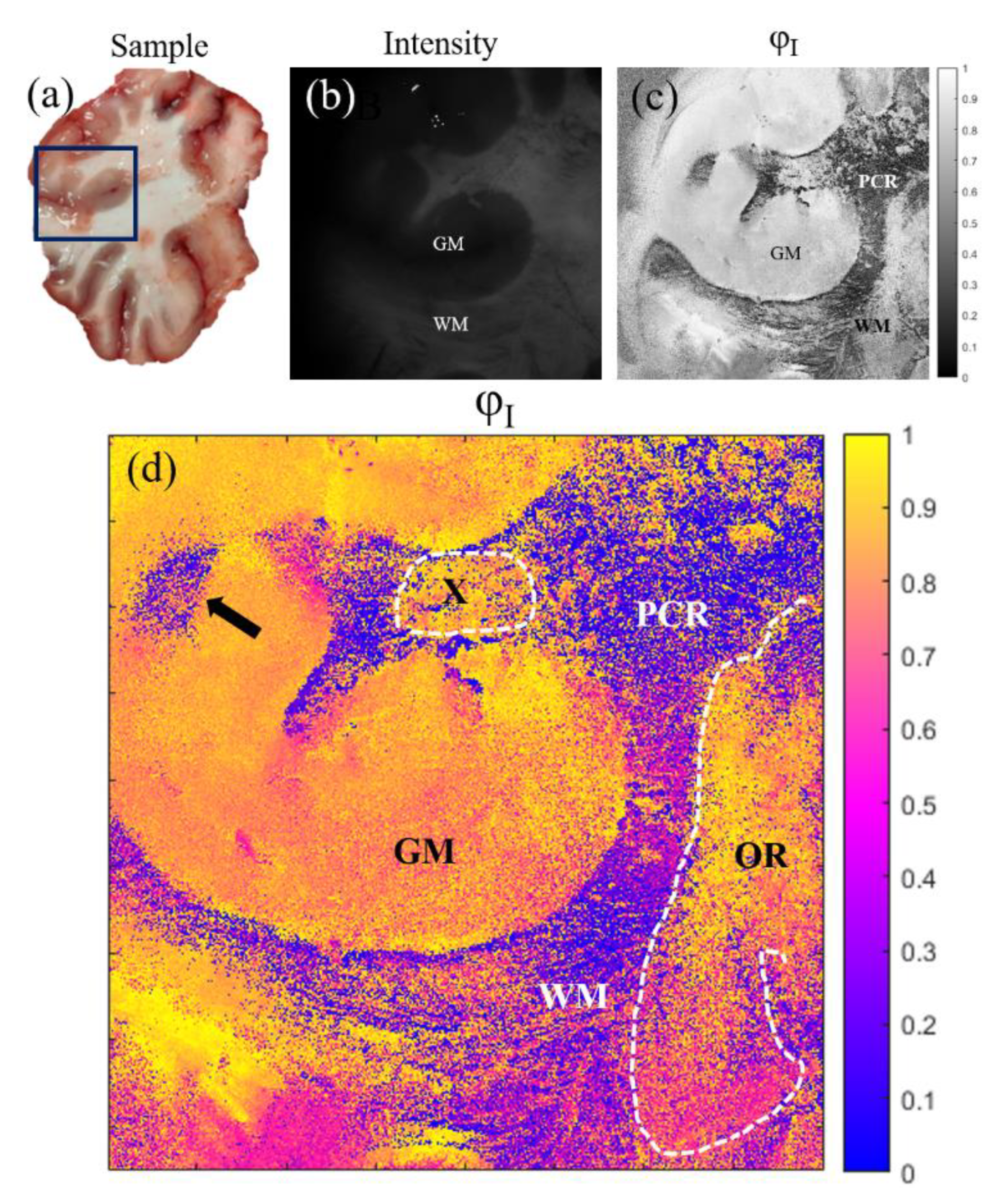
Finally, in Figure 6 we provide the results for a coronal section of a cow brain (see a photography of the sample in Figure 6 (a)). Once again, comparison is set between standard intensity image (Figure 6 (b)) and the best results for polarimetric images (azimuth of the entrance retarder, ; Figure 6 (c) and (d)). In this vein, in Figure 6 (a) and (b) we can see two different structures in the brain: the gray matter (GM) and the white matter (WM); which present different composition and functions in the brain. However, in the polarimetric images (Figure 6 (c) and (d)) we are able to distinguish information about the sample structure which is not visible in the intensity channel. Firstly, the boundaries of the WM and GM are better observed in the image, where we can see a region of WM (see black arrow in Figure 6 (d)) clearly contrasted (note that this WM region is not distinguished in the intensity image and can be misclassified as GM). Importantly, other interesting structures are revealed in the image. In particular, in Figure 6 (d) we can identify fiber tracts of the subcortical WM classified according their directionality. This allows tracing the borders between the longitudinal (at this level) parietal radiations of the corona radiata (PCR in the figure), optical radiations (transversal, OR in the figure) and specific fascicles probably corresponding to the dorsal visual processing pathway (for example, X in the figure). Note that WM is composed by bundles of nerve fibers whose directionality is not identifiable macroscopically or with routine histochemistry, while specific techniques are time consuming or not easily reproducible. However, as we are sensible to different directionalities of the fibers composing the WM through the entrance retarder azimuth, , this channel leads to high contrast of these structures. Therefore, with this channel we are capable to detect information of the directionality of the fibers by means of macroscopic and nondestructive measures of the sample.
7. Conclusions
In this work, we analyzed the suitability of a particular set of polarimetric observables in the framework of biological imaging. Although a wide number of polarimetric observables have been reported as an interesting tool for biomedical and botanical applications, those observables derived from the arrow decomposition are studied for the first time in this work. In particular, the arrow decomposition of a Mueller matrix of a given sample allows for decoupling sixteen meaningful and significant independent polarimetric properties: the mean intensity coefficient () of , three angles (azimuth, ellipticity and retardance) determining the entrance and exit retarders, respectively , three parameters (azimuth, ellipticity and diattenuation) determining the diattenuation vector , three parameters (azimuth, ellipticity and polarizance) determining the polarizance vectorand the three indices of polarimetric purity. These sixteen polarimetric properties are reviewed in this work in section 3 and further applied for imaging three different biological samples in section 4: a Vitis rupestris leaf, a tendinous tissue from a chicken leg and a coronal section of a cow brain. In all cases, some of the arrow decompositions derived observables leading to a significant enhancement of the visualization when compared with standard intensity images. In some cases, these properties even lead to reveal biological structures not visible in the intensity channel.
In the case of the Vitis rupestris leaf, the entrance retardance parameter leads to the best visualization results, allowing for a clear visualization of the necrotic areas of the leaf. For the case of tendinous tissue, the best visualization is provided by the azimuth of the diattenuation , providing the dichroic nature of the tissue and allowing for detecting the boundaries between different fascicles inside the same tendon. Finally, for the coronal section of the brain, the azimuth of the entrance retardancewas selected, this channel revealing fiber tracts of the subcortical white matter classified according to their directionality. These results offer new possibilities to early detection of some pathologies or to fundamental physiological studies. Importantly, we want to highlight that with this technique we are able to clearly observe some structures, as it is the case of different bundles within the subcortical white matter of the brain, which are difficult to describe both in vivo and postmortem and require time-consuming and not easily reproducible methods, such as microinjections or specific, highly destructive, techniques for dissection.
Summarizing, we have demonstrated the excellent potential of these metrics to not only enhance the contrast between different relevant structures in biological samples (both of animal and vegetal origin), but also to show structures that are hidden by using basic imaging systems. These are very promising results in biological applications as in plant pathology detection or animal tissue recognition, the latter paving the way to further studies in human scenarios. These polarimetric methods can be combined with other well-known optical techniques for helping to the early detection of pathologies.
Funding
This research was funded by Ministerio de Ciencia e Innovación and Fondos FEDER (PID2021-126509OB-C21 and PDC2022-133332-C21), Generalitat de Catalunya (2021SGR00138) and Beatriu de Pinós Fellowship (2021-BP-00206).
Informed Consent Statement
Not applicable.
Conflicts of Interest
The authors declare no conflict of interest
References
- Goldstein, D.; Goldstein, D.H. Polarized Light, Revised and Expanded; CRC Press, 2003; ISBN 9780203911587.
- Gil, J.J.; Ossikovski, R. Polarized Light and the Mueller Matrix Approach; CRC Press: New York, 2022; ISBN 9780367815578. [Google Scholar]
- Chipman, R.A. Polarimetry. Chapter 22 in Handbook of Optics II 1995.
- Sheppard, C.J.R.; Bendandi, A.; Le Gratiet, A.; Diaspro, A. Eigenvectors of Polarization Coherency Matrices. Journal of the Optical Society of America A 2020, 37, 1143. [Google Scholar] [CrossRef] [PubMed]
- Van Eeckhout, A.; Lizana, A.; Garcia-Caurel, E.; Gil, J.J.; Sansa, A.; Rodríguez, C.; Estévez, I.; González, E.; Escalera, J.C.; Moreno, I.; et al. Polarimetric Imaging of Biological Tissues Based on the Indices of Polarimetric Purity. J Biophotonics 2018, 11, e201700189. [Google Scholar] [CrossRef] [PubMed]
- Badieyan, S.; Ameri, A.; Razzaghi, M.R.; Rafii-Tabar, H.; Sasanpour, P. Mueller Matrix Imaging of Prostate Bulk Tissues; Polarization Parameters as a Discriminating Benchmark. Photodiagnosis Photodyn Ther 2019, 26, 90–96. [Google Scholar] [CrossRef] [PubMed]
- Van Eeckhout, A.; Garcia-Caurel, E.; Ossikovski, R.; Lizana, A.; Rodríguez, C.; González-Arnay, E.; Campos, J. Depolarization Metric Spaces for Biological Tissues Classification. J Biophotonics 2020, 13. [Google Scholar] [CrossRef] [PubMed]
- Ivanov, D.; Dremin, V.; Borisova, E.; Bykov, A.; Novikova, T.; Meglinski, I.; Ossikovski, R. Polarization and Depolarization Metrics as Optical Markers in Support to Histopathology of Ex Vivo Colon Tissue. Biomed Opt Express 2021, 12, 4560. [Google Scholar] [CrossRef]
- Pierangelo, A.; Benali, A.; Antonelli, M.-R.; Novikova, T.; Validire, P.; Gayet, B.; De Martino, A. Ex-Vivo Characterization of Human Colon Cancer by Mueller Polarimetric Imaging. Opt Express 2011, 19, 1582. [Google Scholar] [CrossRef]
- Rodríguez, C.; Van Eeckhout, A.; Ferrer, L.; Garcia-Caurel, E.; González-Arnay, E.; Campos, J.; Lizana, A. Polarimetric Data-Based Model for Tissue Recognition. Biomed Opt Express 2021, 12, 4852. [Google Scholar] [CrossRef]
- Wan, J.; Dong, Y.; Xue, J.-H.; Lin, L.; Du, S.; Dong, J.; Yao, Y.; Li, C.; Ma, H. Polarization-Based Probabilistic Discriminative Model for Quantitative Characterization of Cancer Cells. Biomed Opt Express 2022, 13, 3339. [Google Scholar] [CrossRef]
- Canabal-Carbia, M.; Van Eeckhout, A.; Rodríguez, C.; González-Arnay, E.; Estévez, I.; Gil, J.J.; García-Caurel, E.; Ossikovski, R.; Campos, J.; Lizana, A. Depolarizing Metrics in the Biomedical Field: Vision Enhancement and Classification of Biological Tissues. J Innov Opt Health Sci 2023. [Google Scholar] [CrossRef]
- Chue-Sang, J.; Holness, N. Use of Mueller Matrix Colposcopy in the Characterization of Cervical Collagen Anisotropy. J Biomed Opt 2018, 23, 1. [Google Scholar] [CrossRef]
- Sprenger, J.; Murray, C.; Lad, J.; Jones, B.; Thomas, G.; Nofech-Mozes, S.; Khorasani, M.; Vitkin, A. Toward a Quantitative Method for Estimating Tumour-Stroma Ratio in Breast Cancer Using Polarized Light Microscopy. Biomed Opt Express 2021, 12, 3241. [Google Scholar] [CrossRef]
- Van Eeckhout, A.; Garcia-Caurel, E.; Garnatje, T.; Escalera, J.C.; Durfort, M.; Vidal, J.; Gil, J.J.; Campos, J.; Lizana, A. Polarimetric Imaging Microscopy for Advanced Inspection of Vegetal Tissues. Sci Rep 2021, 11, 3913. [Google Scholar] [CrossRef] [PubMed]
- Van Eeckhout, A.; Garcia-Caurel, E.; Garnatje, T.; Durfort, M.; Escalera, J.C.; Vidal, J.; Gil, J.J.; Campos, J.; Lizana, A. Depolarizing Metrics for Plant Samples Imaging. PLoS One 2019, 14, e0213909. [Google Scholar] [CrossRef] [PubMed]
- Savenkov, S.N.; Muttiah, R.S.; Oberemok, E.A.; Priezzhev, A.V.; Kolomiets, I.S.; Klimov, A.S. Measurement and Interpretation of Mueller Matrices of Barley Leaves. Quantum Elec (Woodbury) 2020, 50, 55–60. [Google Scholar] [CrossRef]
- Bugami, B. Al; Su, Y.; Rodríguez, C.; Lizana, A.; Campos, J.; Durfort, M.; Ossikovski, R.; Garcia-Caurel, E. Characterization of Vine, Vitis Vinifera, Leaves by Mueller Polarimetric Microscopy. Thin Solid Films 2023, 764, 139594. [Google Scholar] [CrossRef]
- Rodríguez, C.; Van Eeckhout, A.; Garcia-Caurel, E.; Lizana, A.; Campos, J. Automatic Pseudo-Coloring Approaches to Improve Visual Perception and Contrast in Polarimetric Images of Biological Tissues. Sci Rep 2022, 12, 18479. [Google Scholar] [CrossRef]
- Patty, C.H.L.; Luo, D.A.; Snik, F.; Ariese, F.; Buma, W.J.; ten Kate, I.L.; van Spanning, R.J.M.; Sparks, W.B.; Germer, T.A.; Garab, G.; et al. Imaging Linear and Circular Polarization Features in Leaves with Complete Mueller Matrix Polarimetry. Biochimica et Biophysica Acta (BBA) - General Subjects 2018, 1862, 1350–1363. [Google Scholar] [CrossRef]
- Schucht, P.; Lee, H.R.; Mezouar, H.M.; Hewer, E.; Raabe, A.; Murek, M.; Zubak, I.; Goldberg, J.; Kovari, E.; Pierangelo, A.; et al. Visualization of White Matter Fiber Tracts of Brain Tissue Sections With Wide-Field Imaging Mueller Polarimetry. IEEE Trans Med Imaging 2020, 39, 4376–4382. [Google Scholar] [CrossRef]
- Canabal-Carbia, M.; Rodriguez, C.; Estévez, I.; Van Eeckout, A.; González-Arnay, E.; García-Caurel, E.; Garnatje, T.; Lizana, A.; Campos, J. Enhancing Biological Tissue Structures Visualization through Polarimetric Parameters. Proceedings of SPIE 1238205; p. 16. [CrossRef]
- Van Eeckhout, A.; González, E.; Escalera, J.C.; Moreno, I.; Campos, J.; Zhang, H.; Ossikovski, R.; Lizana, A.; Garcia-Caurel, E.; Gil, J.J.; et al. Indices of Polarimetric Purity to Enhance the Image Quality in Biophotonics Applications. Proceedings of SPIE 10685; p. 9. [CrossRef]
- Rodríguez-Núñez, O.; Schucht, P.; Hewer, E.; Novikova, T.; Pierangelo, A. Polarimetric Visualization of Healthy Brain Fiber Tracts under Adverse Conditions: Ex Vivo Studies. Biomed Opt Express 2021, 12, 6674. [Google Scholar] [CrossRef]
- Kupinski, M.; Boffety, M.; Goudail, F.; Ossikovski, R.; Pierangelo, A.; Rehbinder, J.; Vizet, J.; Novikova, T. Polarimetric Measurement Utility for Pre-Cancer Detection from Uterine Cervix Specimens. Biomed Opt Express 2018, 9, 5691. [Google Scholar] [CrossRef] [PubMed]
- Ushenko, V.A.; Hogan, B.T.; Dubolazov, A.; Piavchenko, G.; Kuznetsov, S.L.; Ushenko, A.G.; Ushenko, Y.O.; Gorsky, M.; Bykov, A.; Meglinski, I. 3D Mueller Matrix Mapping of Layered Distributions of Depolarisation Degree for Analysis of Prostate Adenoma and Carcinoma Diffuse Tissues. Sci Rep 2021, 11, 5162. [Google Scholar] [CrossRef] [PubMed]
- Du, E.; He, H.; Zeng, N.; Sun, M.; Guo, Y.; Wu, J.; Liu, S.; Ma, H. Mueller Matrix Polarimetry for Differentiating Characteristic Features of Cancerous Tissues. J Biomed Opt 2014, 19, 076013. [Google Scholar] [CrossRef] [PubMed]
- Rodríguez, C.; Garcia-Caurel, E.; Garnatje, T.; Serra i Ribas, M.; Luque, J.; Campos, J.; Lizana, A. Polarimetric Observables for the Enhanced Visualization of Plant Diseases. Sci Rep 2022, 12, 14743. [Google Scholar] [CrossRef] [PubMed]
- Gil, J.J. Transmittance Constraints in Serial Decompositions of Depolarizing Mueller Matrices: The Arrow Form of a Mueller Matrix. Journal of the Optical Society of America A 2013, 30, 701–707. [Google Scholar] [CrossRef]
- Xing, Z.-F. On the Deterministic and Non-Deterministic Mueller Matrix. J Mod Opt 1992, 39, 461–484. [Google Scholar] [CrossRef]
- Lu, S.-Y.; Chipman, R.A. Interpretation of Mueller Matrices Based on Polar Decomposition. Journal of the Optical Society of America A 1996, 13, 1106. [Google Scholar] [CrossRef]
- Robson, B.A. The Theory of Polarization Phenomena; Clarendon Press: Oxford, 1975. [Google Scholar]
- Sekera, Z. Scattering Matrices and Reciprocity Relationships for Various Representations of the State of Polarization. J Opt Soc Am 1966, 56, 1732. [Google Scholar] [CrossRef]
- Schönhofer, A.; Kuball, H.G. Symmetry Properties of the Mueller Matrix. Chem Phys 1987, 115, 159–167. [Google Scholar] [CrossRef]
- Gil, J.J.; Bernabeu, E. Depolarization and Polarization Indices of an Optical System. Optica Acta: International Journal of Optics 1986, 33, 185–189. [Google Scholar] [CrossRef]
- Gil, J.J. Components of Purity of a Mueller Matrix. Journal of the Optical Society of America A 2011, 28, 1578. [Google Scholar] [CrossRef] [PubMed]
- San José, I.; Gil, J.J. Invariant Indices of Polarimetric Purity: Generalized Indices of Purity for n × n Covariance Matrices. Opt Commun 2011, 284, 38–47. [Google Scholar] [CrossRef]
- Gil, J.J. Invariant Quantities of a Mueller Matrix under Rotation and Retarder Transformations. Journal of the Optical Society of America A 2016, 33, 52–58. [Google Scholar] [CrossRef] [PubMed]
- Gil, J.J. Physical Quantities Involved in a Mueller Matrix. In Proceedings of the SPIE 9853; p. 985302. [CrossRef]
- Jacquemoud, S.; Ustin, S. Leaf Optical Properties; Cambridge University Press, 2019; ISBN 9781108686457.
- Mustafa, F.H.; Jaafar, M.S. Comparison of Wavelength-Dependent Penetration Depths of Lasers in Different Types of Skin in Photodynamic Therapy. Indian Journal of Physics 2013, 87, 203–209. [Google Scholar] [CrossRef]
- Wang, L. V.; Coté, G.L.; Jacques, S.L. Special Section Guest Editorial. J Biomed Opt 2002, 7, 278. [Google Scholar] [CrossRef]
- De Silva, N.; Lumyong, S.; Hyde, K.D.; Bulgakov, T.; Philips, A.J.L.; Yan, J. Mycosphere Essays 9: Defining Biotrophs and Hemibiotrophs. Mycosphere 2016, 7, 545–559. [Google Scholar] [CrossRef]
- Szabó, M.; Csikász-Krizsics, A.; Dula, T.; Farkas, E.; Roznik, D.; Kozma, P.; Deák, T. Black Rot of Grapes (Guignardia Bidwellii)—A Comprehensive Overview. Horticulturae 2023, 9, 130. [Google Scholar] [CrossRef]
- Ullrich, C.I.; Kleespies, R.G.; Enders, M.; Koch, E. Biology of the Black Rot Pathogen, Guignardia Bidwellii, Its Development in Susceptible Leaves of Grapevine Vitis Vinifera. Journal für Kulturflanzen 2009, 61, 82–90. [Google Scholar]
- Kuo, K.; Hoch, H.C. The Parasitic Relationship between Phyllosticta Ampelicidaand Vitis Vinifera. Mycologia 1996, 88, 626–634. [Google Scholar] [CrossRef]
- Sommart, U.; Rukachaisirikul, V.; Trisuwan, K.; Tadpetch, K.; Phongpaichit, S.; Preedanon, S.; Sakayaroj, J. Tricycloalternarene Derivatives from the Endophytic Fungus Guignardia Bidwellii PSU-G11. Phytochem Lett 2012, 5, 139–143. [Google Scholar] [CrossRef]
Figure 1.
Arrow decomposition of a Mueller matrix. For any incident polarization state, with Stokes vector S, the effect of any given Mueller matrix M is equivalent to that a serial combination of an entrance retarder , the arrow form associated with M, and an exit retarder .
Figure 1.
Arrow decomposition of a Mueller matrix. For any incident polarization state, with Stokes vector S, the effect of any given Mueller matrix M is equivalent to that a serial combination of an entrance retarder , the arrow form associated with M, and an exit retarder .
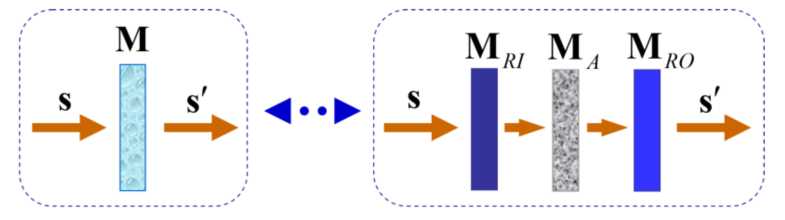
Figure 2.
3D representation of the PSG and PSA optical components. Image reproduced from Ref. [28].
Figure 2.
3D representation of the PSG and PSA optical components. Image reproduced from Ref. [28].
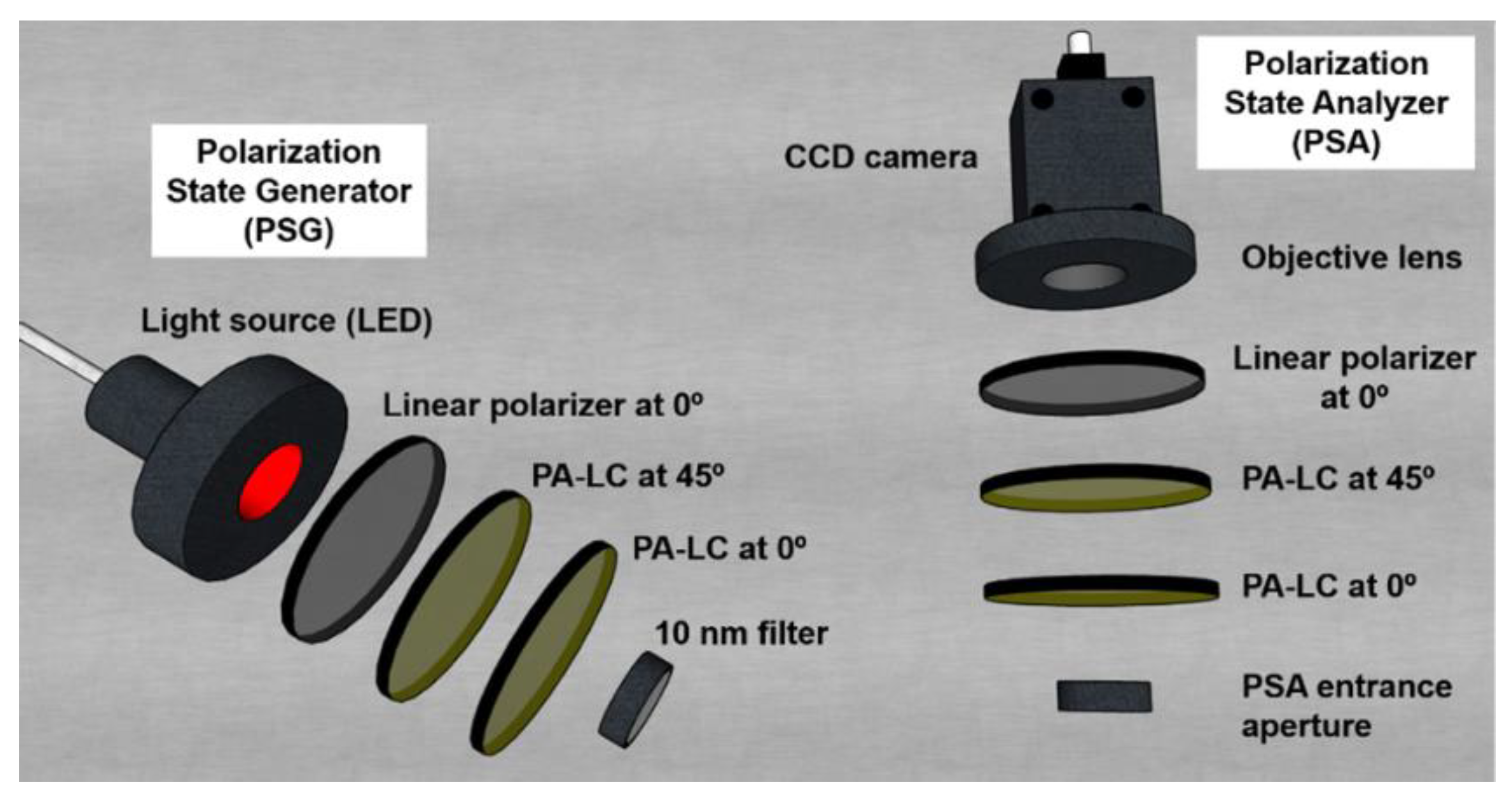
Figure 3.
3D representation of the complete image Mueller polarimeter configurations used in this work: (a) reflection configuration; and (b) transmission configuration. Image reproduced fromRef. [28].
Figure 3.
3D representation of the complete image Mueller polarimeter configurations used in this work: (a) reflection configuration; and (b) transmission configuration. Image reproduced fromRef. [28].
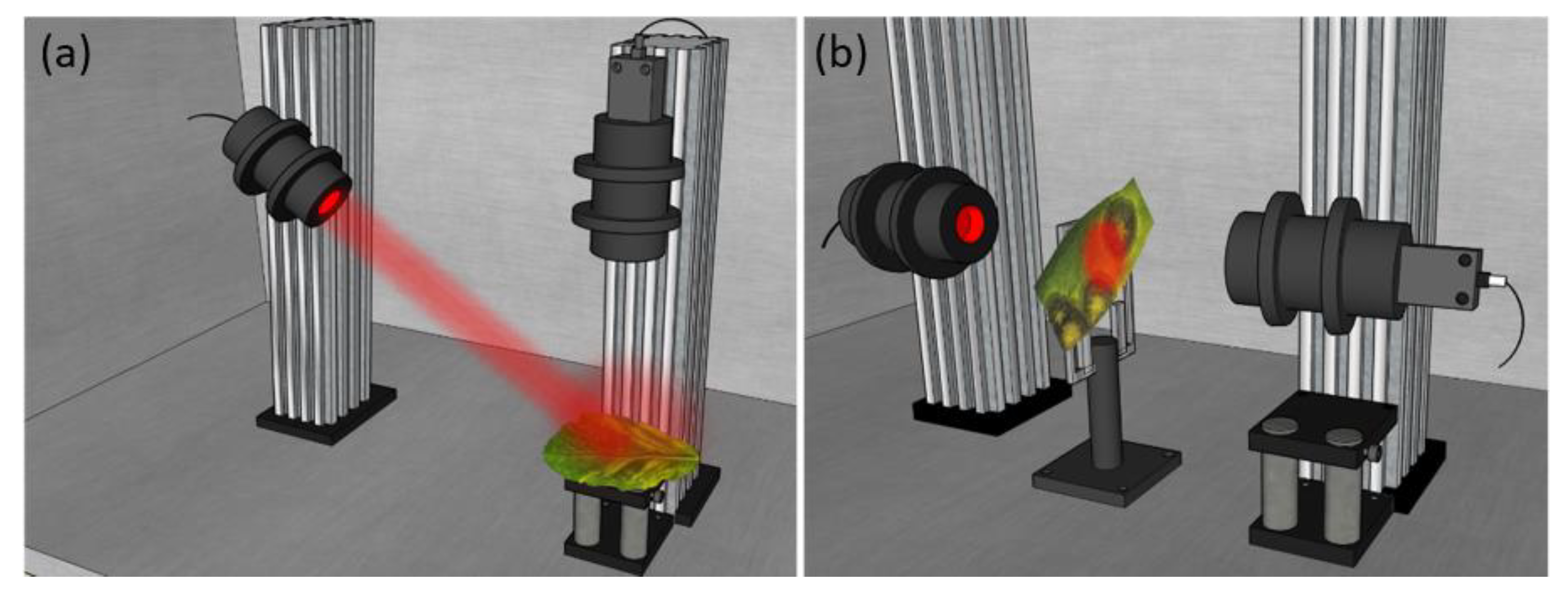
Figure 4.
Images of the pathological grapevine sample for the 470 nm illumination wavelength. (a) Intensity image; (b) and (c) images of the RI polarimetric channel with different colormaps (indicated in the right of the image). The yellow arrows indicate the necrotic lesions of the leaf and, the yellow dashed rectangles indicate some of the primary veins in the leaf.
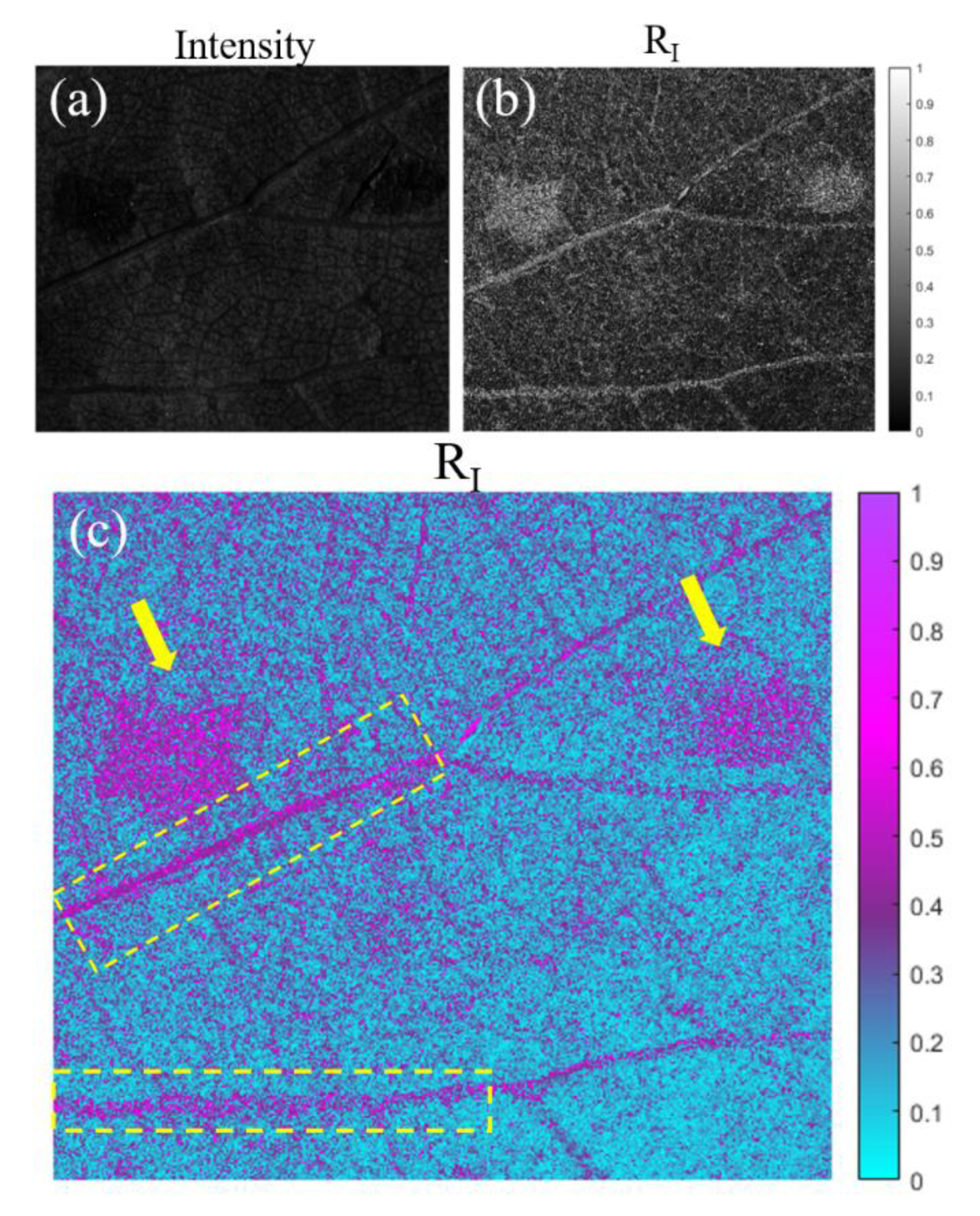
Figure 5.
Images of the tendon sample for the 470 nm illumination wavelength. (a) Intensity image, (b) and (c) azimuth of the diattenuation, , images with different colormaps (indicated in the right of each image). The tendon is partially (*) enveloped by fascia and areolar fatty tissue corresponding to paratenon. Red arrows in (c) indicate boundaries between different fascicles inside the same tendon.
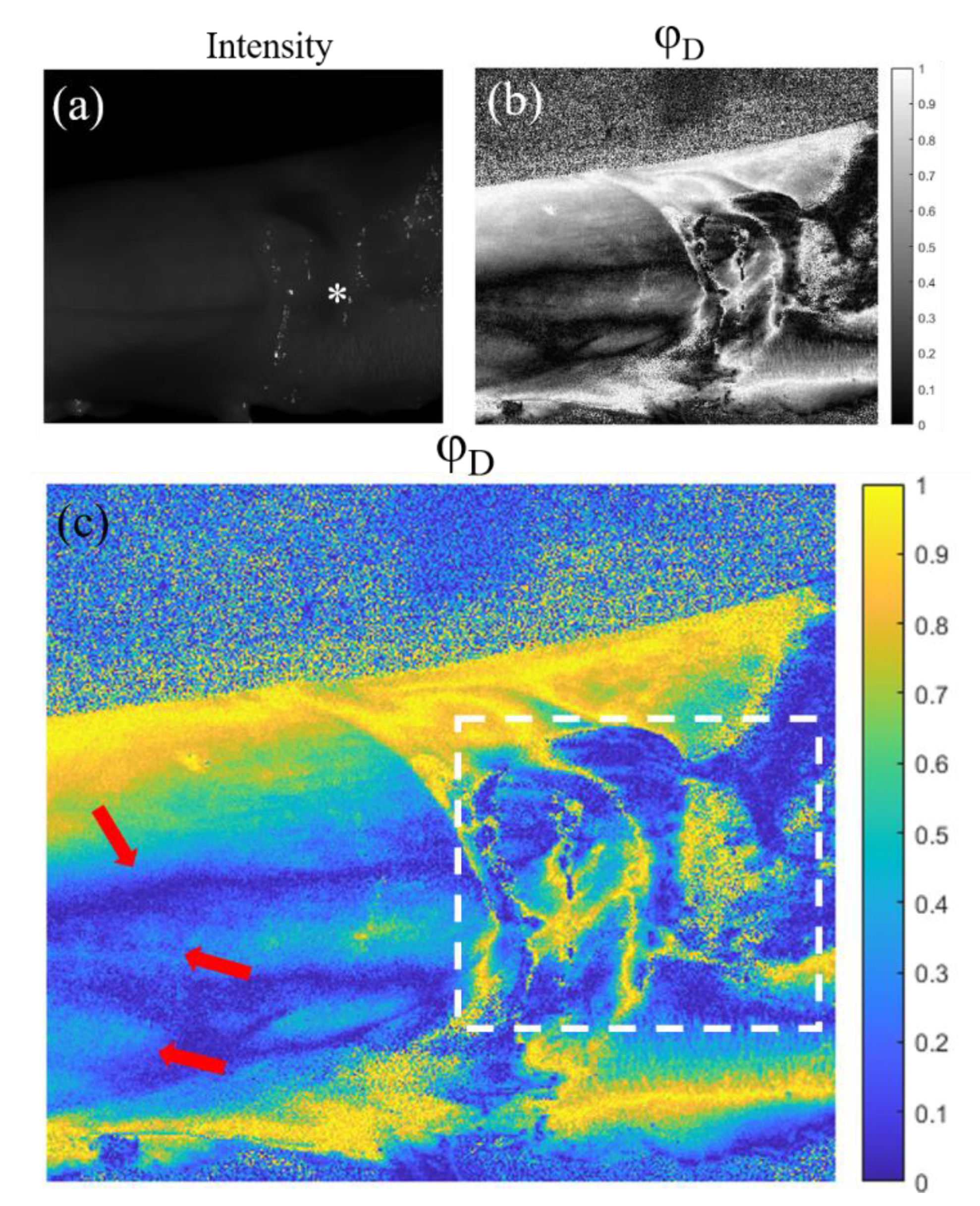
Figure 6.
Images of a coronal section of a cow brain sample for the 470 nm illumination wavelength. The sample corresponds to a section taken in crossroad between the posterior parietal and occipital lobes with cortical grey matter (GM) and subcortical white matter (WM) with fibers correspondent to different types of radiation; parietal radiations of the corona radiate (PCR) and optical radiations (OR). (a) Macroscopic plain view of the full cut of the sample, (b) intensity image, (c) and (d) entrance retarder azimuth images,, with different colormaps (indicated in the right of each image).
Disclaimer/Publisher’s Note: The statements, opinions and data contained in all publications are solely those of the individual author(s) and contributor(s) and not of MDPI and/or the editor(s). MDPI and/or the editor(s) disclaim responsibility for any injury to people or property resulting from any ideas, methods, instructions or products referred to in the content. |
© 2023 by the authors. Licensee MDPI, Basel, Switzerland. This article is an open access article distributed under the terms and conditions of the Creative Commons Attribution (CC BY) license (http://creativecommons.org/licenses/by/4.0/).
Copyright: This open access article is published under a Creative Commons CC BY 4.0 license, which permit the free download, distribution, and reuse, provided that the author and preprint are cited in any reuse.


