Backpropagation and F-adjoint

1. Introduction

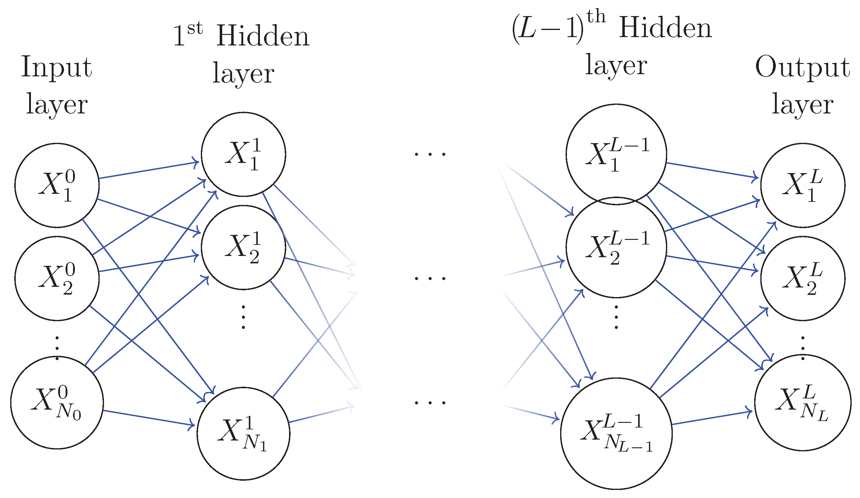
An Artificial Neural Network (ANN) is a mathematical model which is intended to be a universal function approximator which learns from data (cf. McCulloch and Pitts, [1]). In general, an ANN consists of a number of units called artificial neurons, which are a composition of affine mappings, and non-linear (activation) mappings (applied element wise), connected by weighted connections and organized into layers, containing an input layer, one or more hidden layers, and an output layer.The neurons in an ANN can be connected in many different ways. In the simplest cases, the outputs from one layer are the inputs for the neurons in the next layer. An ANN is said to be a feedforward ANN, if outputs from one layer of neurons are the only inputs to the neurons in the following layer. In a fully connected ANN, all neurons in one layer are connected to all neurons in the previous layer (cf. page 24 of [2]). An example of a fully connected feedforward network is presented in Figure 1.

In the present work we focus essentially on feed-forward artificial neural networks, with L hidden layers and a transfer (or activation) function $\sigma$, and the corresponding supervised learning problem. Let us define a simple artificial neural network as follows:

$$X^0=x,Y^h=W^h.X^{h-1},X^h=\sigma \left(Y^h\right),h=1,\cdots ,L$$

(1)

where $x\in {\mathbb{R}}^n$ is the input to the network, h indexes the hidden layer and $W^h$ is the weight matrix of the h-th hidden layer. In what follows we shall refer to the two equations of (1) as the two-step recursive forward formula. The two-step recursive forward formula is very useful in obtaining the outputs of the feed-forward deep neural networks.

A major empirical issue in the neural networks is to estimate the unknown parameters $W^h$ with a sample of data values of targets and inputs. This estimation procedure is characterized by the recursive updating or the learning of estimated parameters. This algorithm is called the backpropagation algorithm. As reviewed by Schmidhuber [3], back-propagation was introduced and developed during the 1970’s and 1980’s and refined by Rumelhart et al. [4]). In addition, it is well known that the most important algorithms of artificial neural networks training is the back-propagation algorithm. From mathematical point view, back-propagation is a method to minimize errors for a loss/cost function through gradient descent. More precisely, an input data is fed to the network and forwarded through the so-called layers ; the produced output is then fed to the cost function to compute the gradient of the associated error. The computed gradient is then back-propagated through the layers to update the weights by using the well known gradient descent algorithm.

As explained in [4], the goal of back-propagation is to compute the partial derivatives of the cost function J. In this procedure, each hidden layer h is assigned teh so-called delta error term ${\delta }^h$. For each hidden layer, the delta error term ${\delta }^h$ is derived from the delta error terms ${\delta }^k,k=h+1,\cdots L$; thus the concept of error back-propagation. The output layer L is the only layer whose error term ${\delta }^L$ has no error dependencies, hence ${\delta }^L$ is then given by the following equation

$${\delta }^L=\frac{\partial J}{\partial W^L}\odot {\sigma }^{\prime }\left(Y^L\right),$$

(2)

where ⊙ denotes the element-wise matrix multiplication (the so-called Hadamard product, which is exactly the element-wise multiplication $"*"$ in Python). For the error term ${\delta }^h$, this term is derived from matrix multiplying ${\delta }^{h+1}$ with the weight transpose matrix $\left(W^{h+1}\right)\top$ and subsequently multiplying (element-wise) the activation function derivative ${\sigma }^{\prime }$ with respect to the preactivation $Y^h$. Thus, one has the following equation

$${\delta }^h={\left(W^{h+1}\right)}^{\top }{\delta }^{h+1}\odot {\sigma }^{\prime }\left(Y^h\right),h=(L-1),\cdots ,1$$

(3)

Once the layer error terms have been assigned, the partial derivative $\frac{\partial J}{\partial W^h}$ can be computed by

$$\frac{\partial J}{\partial W^h}={\delta }^{h+1}{\left(X^h\right)}^{\top }$$

(4)

In particular, we deduce that the back-propagation algorithm is uniquely responsible for computing weight partial derivatives of J by using the recursive equations (4) and (3) with the initialization data given by (2). This procedure is often called "the generalized delta rule". The key question to which we address ourselves in the present work is the following: how could one reformulate this "generalized delta rule" in two-step recursive backward formula as (1) ?

In the present work, we shall provided a concise mathematical answer to the above question. In particular, we shall introduce the so-called two-step rule for back-propagation, recently proposed by the author in [5], similar to the one for forward propagation. Moreover, we explore some mathematical concepts behind the two-step rule for backpropagation.

The rest of the paper is organized as follows. Section 2 outlines some notations, setting and ANN framework. In Section 3 we recall and develop the two-step rule for back-propagation. In Section 4 we introduce the concepts of F-propagation and the associated F-adjoint and rewrite the two-step rule with these notions. In Section 5 we provide some application of this method to study some simple cases. In Section 6 conclusion, related works and mention future work directions are given.

2. Notations, Setting and the ANN

Let us now precise some notations. Firstly, we shall denote any vector $X\in {\mathbb{R}}^n$, is considered as columns $X={\left(X_1,\cdots ,X_n\right)}^{\top }$ and for any family of transfer functions ${\sigma }_i:\mathbb{R}\to \mathbb{R},i=1,\cdots ,n$, we shall introduce the coordinate-wise map $\sigma :{\mathbb{R}}^n\to {\mathbb{R}}^n$ by the following formula

$$\sigma \left(X\right):={\left({\sigma }_1\left(X_1\right),\cdots ,{\sigma }_n\left(X_n\right)\right)}^{\top }.$$

(5)

This map can be considered as an “operator” Hadamard multiplication of columns $\sigma ={\left({\sigma }_1,\cdots ,{\sigma }_n\right)}^{\top }$ and $X={\left(X_1,\cdots ,X_n\right)}^{\top }$, i.e., $\sigma \left(X\right)=\sigma \odot X.$ Secondly, we shall need to recall some useful multi-variable functions derivatives notations. For any $n,m\in {\mathbb{N}}^{*}$ and any differentiable function with respect to the variable x

$$F:\mathbb{R}\ni x\mapsto F\left(x\right)={\left(F_{ij}\left(x\right)\right)}_{\begin{array}{c}1\le i\le m\\ 1\le j\le n\end{array}}\in {\mathbb{R}}^{m\times n}$$

(6)

we use the following notations associated to the partial derivatives of F with respect to x

$$\frac{\partial F}{\partial x}={\left(\frac{\partial F_{ij}\left(x\right)}{\partial x}\right)}_{\begin{array}{c}1\le i\le m\\ 1\le j\le n\end{array}}$$

(7)

In adfdition, for any $n,m\in {\mathbb{N}}^{*}$ and any differentiable function with respect to the matrix variable

$$F:{\mathbb{R}}^{m\times n}\ni X={\left(X_{ij}\right)}_{\begin{array}{c}1\le i\le m\\ 1\le j\le n\end{array}}\mapsto F\left(X\right)\in \mathbb{R}$$

(8)

we shall use the so-called denominator layout notation (see page 15 of [6]) for the partial derivative of F with respect to the matrix X

$$\frac{\partial F}{\partial X}={\left(\frac{\partial F\left(X\right)}{\partial X_{ij}}\right)}_{\begin{array}{c}1\le i\le m\\ 1\le j\le n\end{array}}$$

(9)

In particular, this notation leads to the following useful formulas: for any $q\in {\mathbb{N}}^{*}$ and any matrix $W\in {\mathbb{R}}^{q\times m}$ we have

$$\frac{\partial \left(WX\right)}{\partial X}=W^{\top },$$

(10)

when $X\in {\mathbb{R}}^n$ with $X_n=1$ one has

$$\frac{\partial \left(WX\right)}{\partial X}=W_{♯}^{\top }$$

(11)

where $W_{♯}$ is the matrix W whose last column is removed (this formula is highly useful in practice). Moreover, for any matrix $X\in {\mathbb{R}}^{m\times n}$ we have

$$\frac{\partial \left(WX\right)}{\partial W}=X^{\top }.$$

(12)

Then, by the chain rule one has for any $q,n,m\in {\mathbb{N}}^{*}$ and any differentiable function with respect to the matrices variables $W,X$ :

$$F:(W,X)\mapsto Z:=WX\in {\mathbb{R}}^{q\times n}\mapsto F\left(Z\right)\in \mathbb{R}$$

$$\frac{\partial F}{\partial X}=W^{\top }\frac{\partial F}{\partial Z}\mathrm{and}\frac{\partial F}{\partial W}=\frac{\partial F}{\partial Z}{X}^{\top }.$$

(13)

Furthermore, for any differentiable function with respect to Y

$$F:{\mathbb{R}}^n\ni Y\mapsto X:=\sigma \left(Y\right)\in {\mathbb{R}}^n\mapsto F\left(X\right)\in \mathbb{R}$$

we have

$$\frac{\partial F}{\partial Y}=\frac{\partial F}{\partial X}\odot {\sigma }^{\prime }\left(Y\right).$$

(14)

Throughout this paper, we consider layered feedforward neural networks and supervised learning tasks. Following [2] (see (2.18) in page 24), we will denote such an architecture by

$$A[N_0,\cdots ,N_h,\cdots ,N_L]$$

(15)

where $N_0$ is the size of the input layer, $N_h$ is the size of hidden layer h, and $N_L$ is the size of the output layer; L is defined as the depth of the ANN, then the neural network is called as Deep Neural Network (DNN). We assume that the layers are fully connected, i.e., neurons between two adjacent layers are fully pairwise connected, but neurons within a single layer share no connections.

In the next section we shall recall, develop and improve the two-scale rule for backpropagation, recently introduced by the author in [5].

3. Two-step rule for backpropagation

First, let us mention that the two-step rule for backpropagation is very useful in obtaining some estimation of the unknown parameters $W_h$ with a sample of data values of targets and inputs (see some examples given in [5]).

Now, let ${\alpha }_{ij}^h$ denote the weight connecting neuron j in layer $h-1$ to neuron i in hidden layer h and let the associated transfer function denoted ${\sigma }_i^h$. In general, in the application two different passes of computation are distinguished. The first pass is referred to as the forward pass, and the second is referred to as the backward pass. In the forward pass, the synaptic weights remain fixed throughout the network, and the output $X_i^h$ of neuron i in hidden layer h is computed by the following recursive-coordinate form :

$$X_i^h:={\sigma }_i^h\left(Y_i^h\right)\mathrm{where}{Y}_i^h:=\sum _{j=1}^{N_{h-1}}{\alpha }_{ij}^h{X}_j^{h-1}$$

(16)

In two-step recursive-matrix form, one may rewrite the above formulas as

$$X^h={\sigma }^h\left(Y^h\right)\mathrm{where}{Y}^h=W^h{X}^{h-1},$$

(17)

with

$${\sigma }^h:={({\sigma }_1^h,\cdots ,{\sigma }_{N_h}^h)}^T,W^h:=\left({\alpha }_{ij}^h\right)\in {\mathbb{R}}^{N_h}\times {\mathbb{R}}^{N_{h-1}}.$$

(18)

Let us assume that for all $h\in \{1,\cdots ,L\}$, ${\sigma }^h={(\sigma ,\cdots ,\sigma )}^{\top }$, where $\sigma$ is a fixed activation function, and define a simple artificial neural network as follows:

$$\mathrm{given}{X}^0=x,\mathrm{for}h=1,\cdots ,L,Y^h=W^h.X^{h-1},X^h=\sigma \left(Y^h\right).$$

(19)

where $x\in {\mathbb{R}}^n$ is the input to the network.

To optimize the neural network, we compute the partial derivatives of the cost $J(.)$ w.r.t. the weight matrices $\frac{\partial J(.)}{\partial W^h}$. This quantity can be computed by making use of the chain rule in the back-propagation algorithm. To compute the partial derivative with respect to the matrices variables $\{X^h,Y^h,W^h\}$, we put

$$X_{*}^h=\frac{\partial J(.)}{\partial X^h},Y_{*}^h=\frac{\partial J(.)}{\partial Y^h},{\delta }_{W^h}=\frac{\partial J(.)}{\partial W^h}.$$

(20)

Figure 1. Example of an $A[N_0,\cdots ,N_L]$ architechture.

Figure 1. Example of an $A[N_0,\cdots ,N_L]$ architechture.

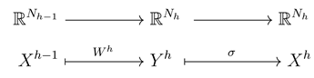
Let us notice that the forward pass computation between the two adjacent layers $h-1$ and h may be represented mathematically as the composition of the following two maps:

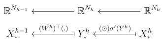
The backward computation between the two adjacent layers h and $h-1$ may be represented mathematically as follows:

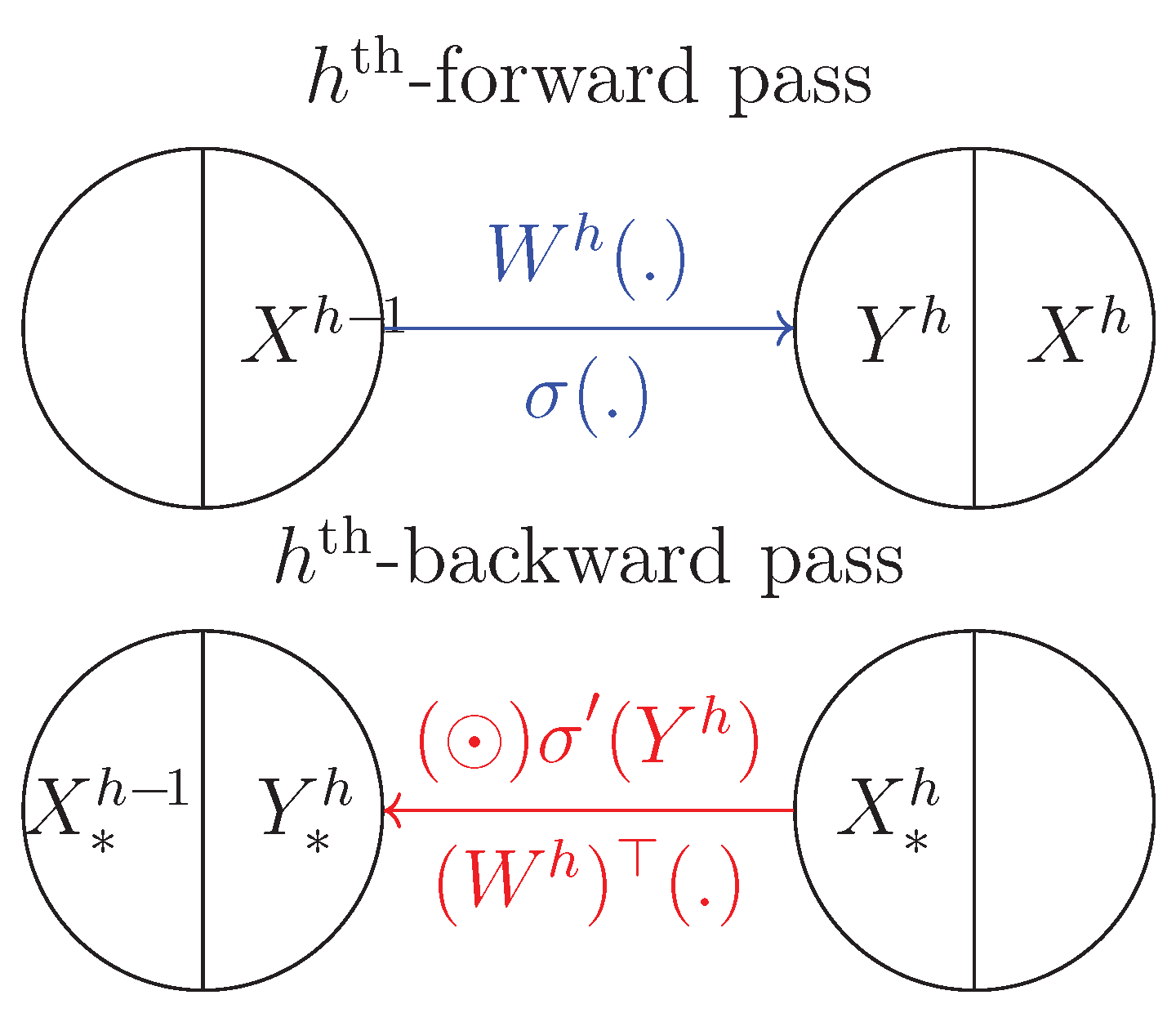
One may represent those maps as a simple mapping diagrams with $X^{h-1}$ and $X_{*}^h$ as inputs and the respective outputs are $Y^h=W^h{X}^{h-1},X^h=\sigma \left(Y^h\right)$ and $Y_{*}^h,X_{*}^{h-1}$ (see Figure 2).

Remark 1. 

It is crucial to remark that, if we impose the following setting on $X^h,W^h$ and ${\sigma }_{N_h}^h$:

1. 

all input vectors have the form $X^h={[X_1^h,\cdots ,X_{N_h-1}^h,1]}^{\top }$ for all $0\le h\le (L-1)$;

2. 

the last functions ${\sigma }_{N_h}^h$ in the columns ${\sigma }^h$ for all $1\le h\le (L-1)$ are constant functions equal to 1.

Then, the $A[N_0,\cdots ,N_L]$ neural network will be equivalent to a $(L-1)$-layered affine neural network with $(N_0-1)$-dimensional input and $N_L$-dimensional output. Each hidden layer h will contain $(N_h-1)$ “genuine” neurons and one (last) “formal”, associated to the bias; the last column of the matrix $W^h$ will be the bias vector for the h-th layer (For more details, see the examples given in Section 5).

Figure 2. Mapping diagrams associated to the forward and backward passes between two adjacent layers.

Figure 2. Mapping diagrams associated to the forward and backward passes between two adjacent layers.

Now, we state our first main mathematical result to answer the above question, in the following theorem.

Theorem 1

(The two-step rule for backpropagation).

Let L be the depth of a Deep Neural Network and $N_h$ the number of neurons in the h-th hidden layer. We denote by $X^0\in {\mathbb{R}}^{N_0}$ the inputs of the network, $W^h\in {\mathbb{R}}^{N_h\times N_{h-1}}$ the weights matrix defining the synaptic strengths between the hidden layer h and its preceding $h-1$. The output $Y^h$ of the hidden layer h are thus defined as follows:

$$X^0=x,Y^h=W^h{X}^{h-1},X^h=\sigma \left(Y^h\right),h=1,2,\cdots ,L.$$

(21)

Where $\sigma (.)$ is a point-wise differentiable activation function. We will thus denote by ${\sigma }^{\prime }(.)$ its first order derivative, $x\in {\mathbb{R}}^{N_0}$ is the input to the network and $W^h$ is the weight matrix of the h-th layer. To optimize the neural network, we compute the partial derivatives of the loss $J\left(f\right(x),y)$ w.r.t. the weight matrices $\frac{\partial J\left(f\right(x),y)}{\partial W^h}$, with $f\left(x\right)$ and y are the output of the DNN and the associated target/label respectively. This quantity can be computed similarly by the following two-step rule:

$${\displaystyle X_{*}^L=\frac{\partial J\left(f\right(x),y)}{\partial X^L},Y_{*}^h=X_{*}^h\odot {\sigma }^{\prime }\left(Y^h\right),X_{*}^{h-1}={\left(W^h\right)}^{\top }{Y}_{*}^h,h=L,\cdots ,1.}$$

(22)

Once $Y_{*}^h$ is computed, the weights update can be computed as

$$\frac{\partial J\left(f\right(x),y)}{\partial W^h}=Y_{*}^h{\left(X^{h-1}\right)}^{\top }.$$

(23)

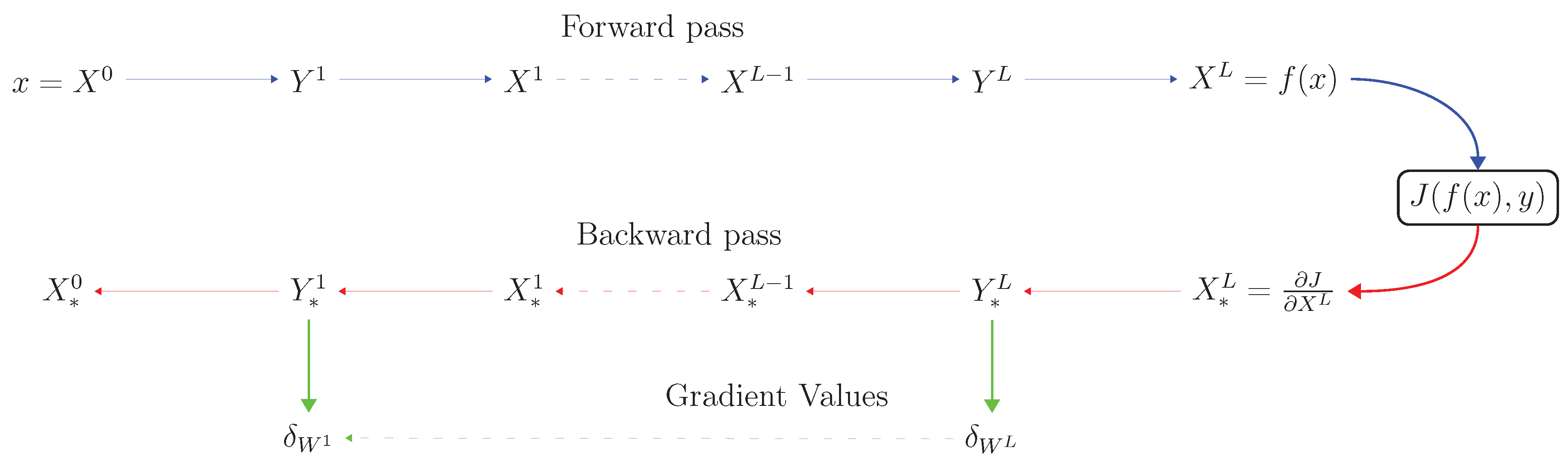
Hereafter, the two-step recursive formulae given in (22) and (23) will be referred to as "the two-step rule for back-propagation" (see the mapping diagram represented by Figure 3.). In particular, this rule provide us a simplified formulation of the so-called "generalized delta rule" similarly to (1). Thus, we have answered our key question.

Proof. 

Firstly, for any$h=1,\cdots ,L$ let us recall the simplified notations introduced by (20):

$$X_{*}^h=\frac{\partial J\left(f\right(x),y)}{\partial X^h},Y_{*}^h=\frac{\partial J\left(f\right(x),y)}{\partial Y^h}.$$

Secondly, for fixed $h\in \{1,\cdots ,L\}$, $X^h=\sigma \left(Y^h\right)$, then (14) implies that

$$\frac{\partial J\left(f\right(x),y)}{\partial Y^h}=\frac{\partial J\left(f\right(x),y)}{\partial X^h}\odot {\sigma }^{\prime }\left(Y^h\right)$$

thus

$$Y_{*}^h=X_{*}^h\odot {\sigma }^{\prime }\left(Y^h\right).$$

(24)

On the other hand, $Y^h=W^h{X}^{h-1}$, thus

$$\frac{\partial J\left(f\right(x),y)}{\partial X^{h-1}}={\left(W^h\right)}^{\top }\frac{\partial J\left(f\right(x),y)}{\partial Y^h}$$

by vertue of (13). As consequence,

$$X_{*}^{h-1}={\left(W^h\right)}^{\top }{Y}_{*}^h.$$

(25)

Equations (24) and (25) implies immediately (22). Moreover, we apply again (13) to the cost function J and the relation $Y^h=W^h{X}^{h-1}$, we deduce that

$$\frac{\partial J\left(f\right(x),y)}{\partial W^h}=\frac{\partial J\left(f\right(x),y)}{\partial Y^h}{\left(X^{h-1}\right)}^{\top }=Y_{*}^h{\left(X^{h-1}\right)}^{\top }.$$

This end the proof of the Theorem 1. Furthermore, in the practical setting mentioned in Remark 1, one should replace $W^h$ by $W_{♯}^h$ by vertue of (11). Thus, we have for all $h\in \{L,\cdots ,2\}$

$${\displaystyle X_{*}^{h-1}={\left(W_{♯}^h\right)}^{\top }{Y}_{*}^h,}$$

and then the associated two-step rule is given by

$${\displaystyle X_{*}^L=\frac{\partial J\left(f\right(x),y)}{\partial X^L},Y_{*}^h=X_{*}^h\odot {\sigma }^{\prime }\left(Y^h\right),X_{*}^{h-1}={\left(W_{♯}^h\right)}^{\top }{Y}_{*}^h,h=L,\cdots ,1.}$$

(26)

□

4. The F-propagation and F-adjoint

Based on the above idea of two-scale rule for back-prpagation, we shall introduce the following two natural definitions :

Definition 1

(An F-propagation).

Le $X^0\in {\mathbb{R}}^{N_0}$ be a given data, σ be a coordinate-wise map from ${\mathbb{R}}^{N_h}$ into ${\mathbb{R}}^{N_{h+1}}$ and $W^h\in {\mathbb{R}}^{N_h\times N_{h-1}}$ for all $1\le h\le L$. We say that we have a two-step recursive F-propagation F through the DNN $A[N_0,\cdots ,N_L]$ if one has the following family of vectors

$$F:=\left\{\begin{array}{c}{X}^0,Y^1,X^1,\cdots ,X^{L-1},Y^L,X^L\end{array}\right\}$$

(27)

with

$$Y^h=W^h{X}^{h-1},X^h=\sigma \left(Y^h\right),X^h\in {\mathbb{R}}^{N_h},h=1,\cdots ,L.$$

(28)

Before going further, let us point that in the above definition the prefix "F" stands for "Feed-forward".

Definition 2

(The F-adjoint of an F-propagation).

Let $X_{*}^L\in {\mathbb{R}}^{N_L}$ be a given data and a two-step recursive F-propagation F through the DNN $A[N_0,\cdots ,N_L]$. We define the F-adjoint $F_{*}$ of the F-propagation F as follows

$$F_{*}:=\left\{\begin{array}{c}{X}_{*}^L,Y_{*}^L,X_{*}^{L-1},\cdots ,X_{*}^1,Y_{*}^1,X_{*}^0\end{array}\right\}$$

(29)

with

$$Y_{*}^h=X_{*}^h\odot {\sigma }^{\prime }\left(Y^h\right),X_{*}^{h-1}={\left(W^h\right)}^{\top }{Y}_{*}^h,h=L,\cdots ,1.$$

(30)

Remark 2.

It is immediately seen that if for every $h=1,\cdots ,L$, $W^h$ is an orthogonal matrix i.e. ${\left(W^h\right)}^{\top }{W}^h=W^h{\left(W^h\right)}^{\top }=I_{N_h}$, $\sigma \left(X\right)=X$ and $X^0=X_{*}^0$ one has

$$Y^1=W^1{X}_{*}^0=W^1{\left(W^1\right)}^{\top }{Y}_{*}^1=Y_{*}^1,$$

$$Y^2=W^2{X}_{*}^1=W^2{\left(W^2\right)}^{\top }{Y}_{*}^2=Y_{*}^2,$$

by recurrence we obtain

$$Y^L=W^L{X}_{*}^{L-1}=W^L{\left(W^L\right)}^{\top }{Y}_{*}^L=Y_{*}^L.$$

On the other hand,

$$X^1=\sigma \left(W^L{X}^0\right)=W^L{X}_{*}^0=Y_{*}^1=X_{*}^1,$$

also, by recurrence we get

$$X^L=W^L{X}^{L-1}=W^L{\left(W^L\right)}^{\top }{Y}_{*}^L=Y_{*}^L=X_{*}^L.$$

Consequently, we obtain $F_{*}=F$ and we refer to this property as F-symmetric. We may conjecture that under the following assumption : for all vector X, $\sigma \left(X\right)=X$, a DNN is F-symmetric if and only if ${\left(W^h\right)}^{\top }{W}^h=W^h{\left(W^h\right)}^{\top }=I_{N_h},h=1,\cdots L$, i.e. for all $h=1,\cdots ,L$, $W^h$ is an orthogonal matrix.

Similarly to the note at the end of the proof of Theorem 1, if we are in the practical setting mentioned in Remark 1, one should replace $W^h$ by $W_{♯}^h$ by vertue of (11) and (30) by the following relations :

$${\displaystyle Y_{*}^h=X_{*}^h\odot {\sigma }^{\prime }\left(Y^h\right),X_{*}^{h-1}={\left(W_{♯}^h\right)}^{\top }{Y}_{*}^h,h=L,\cdots ,1.}$$

(31)

Now, following these definitions, we can deduce our second main mathematical result.

Theorem 2

(The backpropagation is an F-adjoint of the associated F-propagation).

Let $A[N_0,\cdots ,N_L]$ be a Deep Neural Network and let $F:=\left\{\begin{array}{c}{X}^0,Y^1,X^1,\cdots ,X^{L-1},Y^L,X^L\end{array}\right\}$ an F-propagation through $A[N_0,\cdots ,N_L]$, with weights matrix $W^h\in {\mathbb{R}}^{N_h\times N_{h-1}}$ and fixed point-wise activation ${\sigma }^h=\sigma$, $h=1,\cdots ,L$.

Let $X^0=x\in {\mathbb{R}}^{N_0}$ be the input to this network and $J\left(f\right(x),y)$ be the loss function, with $f\left(x\right)$ and y are the output of the DNN and the associated target/label respectively.

Then the associated backpropagation pass is computed with the F-adjoint of F with $X_{*}^L=\frac{\partial J}{\partial X^L}(f\left(x\right),y)$, that is $F_{*}:=\left\{\begin{array}{c}{X}_{*}^L,Y_{*}^L,X_{*}^{L-1},\cdots ,X_{*}^1,Y_{*}^1,X_{*}^0\end{array}\right\}$. Moreprecisely, for all $h=1,\cdots ,L$

$$\frac{\partial J\left(f\right(x),y)}{\partial W^h}=Y_{*}^h{\left(X^{h-1}\right)}^{\top }.$$

Before proving the Theorem 2, let us as remark that this mathematical result is a simplified version of Theorem 1 based on the notion of F-adjoint introduced in Definition 2.

Proof. 

By definition of the F-adjoint one has for all $h=L,\cdots ,1,$

$$Y_{*}^h=X_{*}^h\odot {\sigma }^{\prime }\left(Y^h\right),X_{*}^{h-1}={\left(W^h\right)}^{\top }{Y}_{*}^h.$$

Moreover, by the two-step rule for backpropagation, we have

$${\displaystyle X_{*}^L=\frac{\partial J(.)}{\partial X^L},Y_{*}^h=X_{*}^h\odot {\sigma }^{\prime }\left(Y^h\right),{\delta }_{W^h}=Y_{*}^h{\left(X^{h-1}\right)}^{\top },X_{*}^{h-1}={\left(W^h\right)}^{\top }{Y}_{*}^h,}$$

As consequence, we deduce that the backpropagation is exactely determined by the F-adjoint $F_{*}$ relatively to the choice of ${\displaystyle X_{*}^L=\frac{\partial J(.)}{\partial X^L}}$. Here we present a new proof of Theorem 1 of [5] which is simpler than the original one. □

5. Application to the two simplest cases $A[1,1,1]$ and $A[1,2,1]$

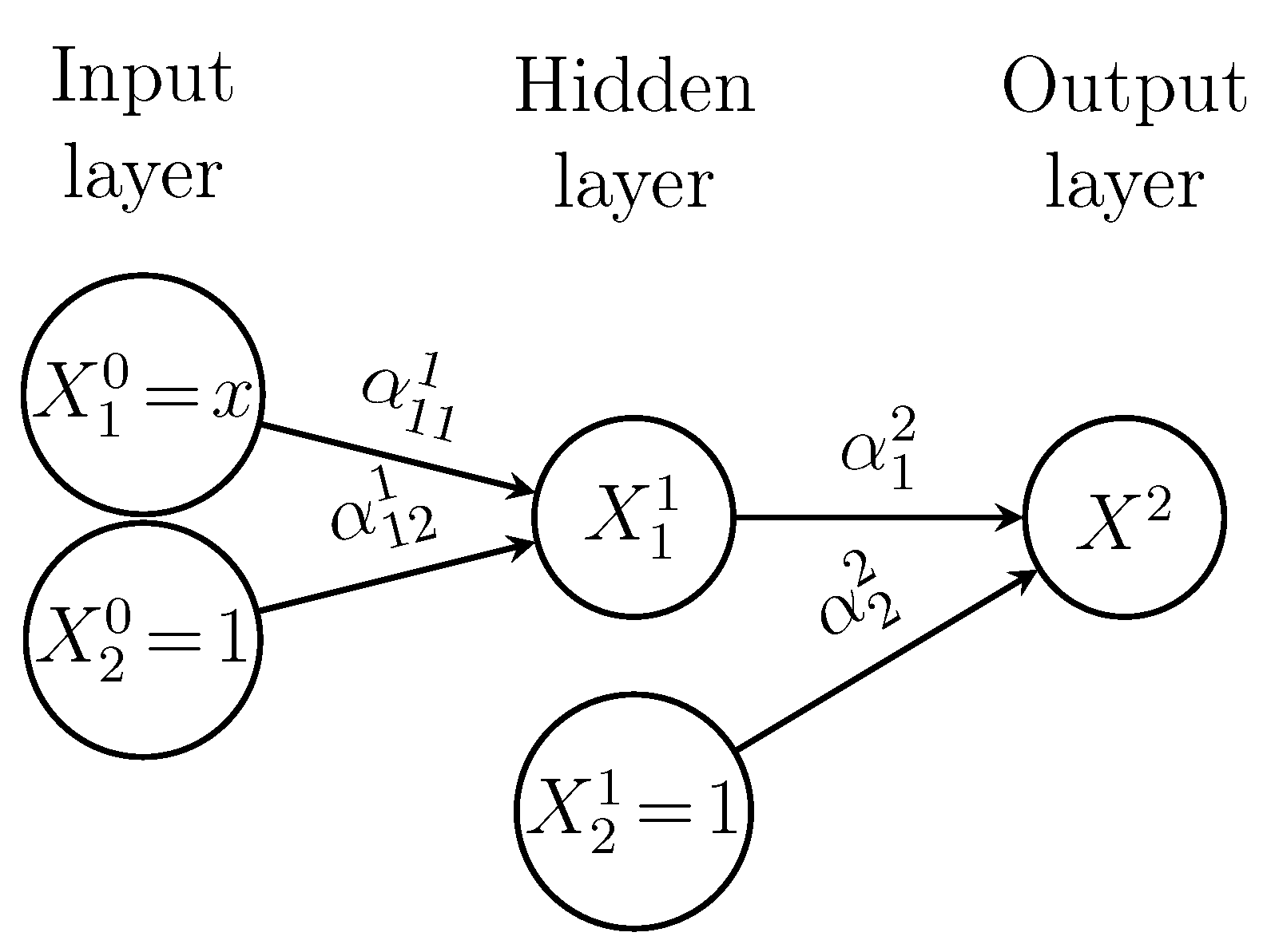
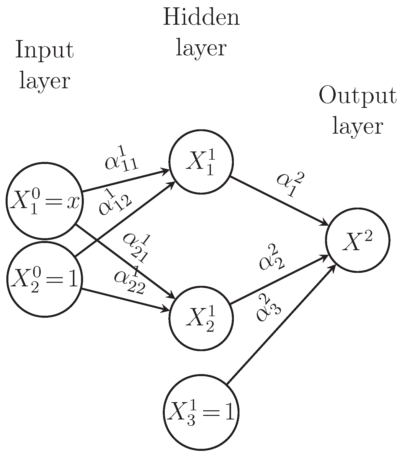
The present section shows that in the following four simplest cases associated to the DNN $A[1,N_1,1]$ with $N_1=1,2$, we shall apply the notion of F-adjoint to compute the partial derivative of the elementary cost function J defined by $J\left(f\right(x),y)=f\left(x\right)-y$ for any real x and fixed real y. In this particular setting, we have the two simplest cases $A[1,1,1]$ and $A[1,2,1]$: one neuron and two neurons in the hidden layer (see Figure 4 and Figure 5).

5.1. The first case: $A[1,1,1]$

The first simplest case corresponds to $A[1,1,1]$ architecture is shows by the Figure 4. Let us denote by a $W^1=\left(\begin{array}{cc}{\alpha }_{11}^1& {\alpha }_{12}^1\end{array}\right)$ and $W^2=\left(\begin{array}{cc}{\alpha }_1^2& {\alpha }_2^2\end{array}\right)$ the weights in the first and second layer. We will evaluate the ${\delta }_{W^1}$ and ${\delta }_{W^2}$ by the differential calculus rules firstly and then recover this result by the two-step rule for back-propagation.

Figure 4. The DNN associated to the case 1.

Figure 4. The DNN associated to the case 1.

The F-propagation through this DNN is given by : 

Obviously, we have

$$X^0=\left(\begin{array}{c}x\\ 1\end{array}\right),Y^1={\alpha }_{11}^{1}x+{\alpha }_{12}^1,X^1=\left(\begin{array}{c}\sigma ({\alpha }_{11}^{1}x+{\alpha }_{12}^1)\\ 1\end{array}\right),$$

$$Y^2={\alpha }_1^2\sigma ({\alpha }_{11}^{1}x+{\alpha }_{12}^1)+{\alpha }_2^2,X^2=\sigma \left[{\alpha }_1^2\sigma ({\alpha }_{11}^{1}x+{\alpha }_{12}^1)+{\alpha }_2^2\right].$$

Let us denote $y^1:={\alpha }_{11}^{1}x+{\alpha }_{12}^1$ and $y^2:={\alpha }_1^2\sigma \left(y^1\right)+{\alpha }_2^2$, then

$$F=\left\{X^0=\left(\begin{array}{c}x\\ 1\end{array}\right),Y^1=y^1,X^1=\left(\begin{array}{c}\sigma \left(y^1\right)\\ 1\end{array}\right),Y^2=y^2,X^2=\sigma \left(y^2\right)\right\}$$

and

$$J(f\left(x\right),y)=X^2-y=\sigma \left(y^2\right)-y=\sigma \left[{\alpha }_1^2\sigma ({\alpha }_{11}^{1}x+{\alpha }_{12}^1)+{\alpha }_2^2\right]-y.$$

Hence, by using the differential calculus rules one gets

$${\delta }_{W^2}={\left(\begin{array}{c}\frac{\partial J}{\partial {\alpha }_1^2}\\ \frac{\partial J}{\partial {\alpha }_2^2}\end{array}\right)}^{\top }={\left(\begin{array}{c}{\sigma }^{\prime }\left(y^2\right)\sigma \left(y^1\right)\\ {\sigma }^{\prime }\left(y^2\right)\end{array}\right)}^{\top },{\delta }_{W^1}={\left(\begin{array}{c}\frac{\partial J}{\partial {\alpha }_{11}^2}\\ \frac{\partial J}{\partial {\alpha }_{12}^2}\end{array}\right)}^{\top }={\left(\begin{array}{c}{\sigma }^{\prime }\left(y^2\right){\sigma }^{\prime }\left(y^1\right){\alpha }_1^{2}x\\ {\sigma }^{\prime }\left(y^2\right){\sigma }^{\prime }\left(y^1\right){\alpha }_1^2\end{array}\right)}^{\top }.$$

(32)

The F-adjoint of the above F-propagation is given by 

$$F_{*}=\left\{X_{*}^2=1,Y_{*}^2={\sigma }^{\prime }\left(y^2\right),X_{*}^1={\alpha }_1^2{\sigma }^{\prime }\left(y^2\right),Y_{*}^1={\alpha }_1^2{\sigma }^{\prime }\left(y^2\right){\sigma }^{\prime }\left(y^1\right),X_{*}^0={\alpha }_{11}^1{\alpha }_1^2{\sigma }^{\prime }\left(y^2\right){\sigma }^{\prime }\left(y^1\right)\right\}$$

since by (31) we have

$${\displaystyle Y_{*}^h=X_{*}^h\odot {\sigma }^{\prime }\left(Y^h\right),X_{*}^{h-1}={\left(W_{♯}^h\right)}^{\top }{Y}_{*}^h,h=2,1}$$

then we deduce that

$$Y_{*}^2=X_{*}^2\odot {\sigma }^{\prime }\left(y^2\right)={\sigma }^{\prime }\left(y^2\right),X_{*}^1={\left(W_{♯}^2\right)}^{\top }{Y}_{*}^2={\alpha }_1^2{\sigma }^{\prime }\left(y^2\right),Y_{*}^1=X_{*}^1\odot {\sigma }^{\prime }\left(y^1\right)={\alpha }_1^2{\sigma }^{\prime }\left(y^2\right){\sigma }^{\prime }\left(y^1\right)$$

and

$$X_{*}^0={\left(W_{♯}^1\right)}^{\top }{Y}_{*}^1={\alpha }_{11}^1{Y}_{*}^1={\alpha }_{11}^1{\alpha }_1^2{\sigma }^{\prime }\left(y^2\right){\sigma }^{\prime }\left(y^1\right)$$

Hence, by using the F-adjoint and the two-step rule (26) one gets

$${\delta }_{W^2}=Y_{*}^2{\left(X^1\right)}^{\top }={\left(\begin{array}{c}{\sigma }^{\prime }\left(y^2\right)\sigma \left(y^1\right)\\ {\sigma }^{\prime }\left(y^2\right)\end{array}\right)}^{\top },{\delta }_{W^1}=Y_{*}^1{\left(X^0\right)}^{\top }={\left(\begin{array}{c}{\sigma }^{\prime }\left(y^2\right){\sigma }^{\prime }\left(y^1\right){\alpha }_1^{2}x\\ {\sigma }^{\prime }\left(y^2\right){\sigma }^{\prime }\left(y^1\right){\alpha }_1^2\end{array}\right)}^{\top }.$$

Thus we recover, via the F-adjoint $F_{*}$, the computation given by (32).

5.2. The second case: $A[1,2,1]$

The second simplest case corresponds to $A[1,2,1]$ architecture is shows by the Figure 5. In this case we have $W^1=\left(\begin{array}{cc}{\alpha }_{11}^1& {\alpha }_{12}^1\\ {\alpha }_{21}^1& {\alpha }_{22}^1\end{array}\right)$ and $W^2=\left(\begin{array}{ccc}{\alpha }_1^2& {\alpha }_2^2& {\alpha }_3^2\end{array}\right)$. Thus, one deduce immediately that

Figure 5. The DNN associated to the case 2.

Figure 5. The DNN associated to the case 2.

The F-propagation through this DNN is given by : 

$$F=\left\{X^0=\left(\begin{array}{c}x\\ 1\end{array}\right),Y^1=\left(\begin{array}{c}{y}_{11}^1\\ y_{21}^1\end{array}\right),X^1=\left(\begin{array}{c}\sigma \left(y_{11}^1\right)\\ \sigma \left(y_{21}^1\right)\\ 1\end{array}\right),Y^2=y^2,X^2=\sigma \left(y^2\right)\right\}$$

Hence, by using the differential calculus rules one gets

$${\delta }_{W^2}={\left(\begin{array}{c}{\sigma }^{\prime }\left(y^2\right)\sigma \left(y_{11}^1\right)\\ {\sigma }^{\prime }\left(y^2\right)\sigma \left(y_{21}^1\right)\\ {\sigma }^{\prime }\left(y^2\right)\end{array}\right)}^{\top },{\delta }_{W^1}=\left(\begin{array}{cc}{\alpha }_1^{2}x{\sigma }^{\prime }\left(y_{11}^1\right){\sigma }^{\prime }\left(y_{21}^1\right)& {\alpha }_1^2{\sigma }^{\prime }\left(y_{11}^1\right){\sigma }^{\prime }\left(y^2\right)\\ {\alpha }_2^{2}x{\sigma }^{\prime }\left(y_{21}^1\right){\sigma }^{\prime }\left(y^2\right)& {\alpha }_2^2{\sigma }^{\prime }\left(y_{21}^1\right){\sigma }^{\prime }\left(y^2\right)\end{array}\right)$$

with

$$y^2:={\alpha }_1^2\sigma \left(w^{1}x\right)+{\alpha }_2^2\sigma \left(w^2\right)+{\alpha }_3^2,y_{11}^1:={\alpha }_{11}^{1}x+{\alpha }_{12}^1,y_{21}^1:={\alpha }_{21}^{1}x+{\alpha }_{22}^1.$$

The F-adjoint of the above F-propagation is given by 

$$F_{*}=\left\{X_{*}^2=1,Y_{*}^2={\sigma }^{\prime }\left(y^2\right),X_{*}^1=\left(\begin{array}{c}{\alpha }_1^2{\sigma }^{\prime }\left(y^2\right)\\ {\alpha }_2^2{\sigma }^{\prime }\left(y^2\right)\end{array}\right),Y_{*}^1=\left(\begin{array}{c}{\alpha }_1^2{\sigma }^{\prime }\left(y^2\right){\sigma }^{\prime }\left(y_{11}^1\right)\\ {\alpha }_2^2{\sigma }^{\prime }\left(y^2\right){\sigma }^{\prime }\left(y_{21}^1\right)\end{array}\right),X_{*}^0=x^0\right\}$$

with $x^0={\alpha }_{11}^1{\alpha }_1^2{\sigma }^{\prime }\left(y^2\right){\sigma }^{\prime }\left(y_{11}^1\right)+{\alpha }_{21}^1{\alpha }_2^2{\sigma }^{\prime }\left(y^2\right){\sigma }^{\prime }\left(y_{21}^1\right)$. As above, by using also the F-adjoint and the two-step rule (26) one gets

$${\delta }_{W^2}=Y_{*}^2{\left(X^1\right)}^{\top }={\left(\begin{array}{c}{\sigma }^{\prime }\left(y^2\right)\sigma \left(y_{11}^1\right)\\ {\sigma }^{\prime }\left(y^2\right)\sigma \left(y_{21}^1\right)\\ {\sigma }^{\prime }\left(y^2\right)\end{array}\right)}^{\top },{\delta }_{W^1}=Y_{*}^1{\left(X^0\right)}^{\top }=\left(\begin{array}{cc}{\alpha }_1^{2}x{\sigma }^{\prime }\left(y_{11}^1\right){\sigma }^{\prime }\left(y^2\right)& {\alpha }_1^2{\sigma }^{\prime }\left(y_{11}^1\right){\sigma }^{\prime }\left(y_{21}^1\right)\\ {\alpha }_2^{2}x{\sigma }^{\prime }\left(y_{21}^1\right){\sigma }^{\prime }\left(y_{21}^1\right)& {\alpha }_2^2{\sigma }^{\prime }\left(y_{21}^1\right){\sigma }^{\prime }\left(y_{21}^1\right)\end{array}\right).$$

6. Related works and Conclusion

To the best of our knowledge, in literature, the related works to this paper are [7] and [8]. In particular, in the first paper the authors uses some decomposition of the partial derivatives of the cost function, similar to the two-step formula (cf. (22)), to replace the standard back-propagation. In addition, they show (experimentally) that for specific scenarios, the two-step decomposition yield better generalization performance than the one based on the standard back-propagation. But in the second article, the authors find some similar update equation similar to the one given by (22) that report similarly to standard back-propagation at convergence. Moreover, this method discovers new variations of the back-propagation by learning new propagation rules that optimize the generalization performance after a few epochs of training.

In conclusion, we have provided a two-step rule for back-propagation similar to the one for forward propagation and a new mathematical notion called F-adjoint which is combined by the two-step rule for back-propagation describes, in a simple and direct way, the computational process given by the back-propagation pass. We hope that, the power and simplicity of the F-adjoint concept may inspire the exploration of novel approaches for optimizing some artificial neural networks training algorithms and investigating some mathematical properties of the F-propagation and F-adjoint notions. As future work, we envision to explore some mathematical results regarding the F-adjoint for deep neural networks with respect to the choice of the activation function.

References

- W. S. McCulloch and W. Pitts, A logical calculus of the ideas immanent in nervous activity. The bulletin of mathematical biophysics 1943, 5, 115–133.
- Baldi, P. Deep learning in science; Cambridge University Press: Cambridge, 2021.
- Schmidhuber, J. Deep learning in neural networks: An overview. Neural networks 2015, 61, 85–117.
- Rumelhart, D.E.; Hinton, G.E.; Williams, R.J. Learning representations by back-propagating errors. nature 1986, 323, 533–536.
- Boughammoura, A. A Two-Step Rule for Backpropagation 2023. Preprint at https://www.preprints.org/manuscript/202303.0001/v3, doi:10.20944/preprints202303.0001.v3. [CrossRef]
- Ye, J.C. Geometry of Deep Learning; Springer: Heidelberg, 2022.
- Alber, M.; Bello, I.; Zoph, B.; Kindermans, P.J.; Ramachandran, P.; Le, Q. Backprop evolution 2018. Preprint at https://arxiv.org/abs/1808.02822.
- Hojabr, R.; Givaki, K.; Pourahmadi, K.; Nooralinejad, P.; Khonsari, A.; Rahmati, D.; Najafi, M.H. TaxoNN: A Light-Weight Accelerator for Deep Neural Network Training. 2020 IEEE International Symposium on Circuits and Systems (ISCAS). IEEE, 2020, pp. 1–5.
Figure 3.
Mapping diagram associated to the two-step rule for backpropagation.
Disclaimer/Publisher’s Note: The statements, opinions and data contained in all publications are solely those of the individual author(s) and contributor(s) and not of MDPI and/or the editor(s). MDPI and/or the editor(s) disclaim responsibility for any injury to people or property resulting from any ideas, methods, instructions or products referred to in the content. |
© 2023 by the authors. Licensee MDPI, Basel, Switzerland. This article is an open access article distributed under the terms and conditions of the Creative Commons Attribution (CC BY) license (http://creativecommons.org/licenses/by/4.0/).
Copyright: This open access article is published under a Creative Commons CC BY 4.0 license, which permit the free download, distribution, and reuse, provided that the author and preprint are cited in any reuse.