3. Wavelet-based measure of time series non-stationarity
Let’s consider a random signal
where
is an integer discrete time index. For a finite sample of the signal entropy could be defined as:
Here
are coefficients of orthogonal wavelet decomposition. Within a finite set of Daubechies wavelet bases [
20] with the number of vanishing moments from 1 to 10 the optimal basis is chosen from the minimum of (1).
The DJ index was introduced in the problem of noise reduction and compression of information by setting all “small” wavelet coefficients to zero and performing an inverse wavelet transform [
14,
20]. This operation of noise reduction is performed for optimal wavelet basis which was found from minimum of entropy. The problem is how define the threshold which separates “large” wavelet coefficients from “small” ones. In [14} this problem was solved using formula of asymptotic probability of the maximum deviations of Gaussian white noise. The DJ threshold is given by the expression
where
is standard deviation of wavelet coefficients of the 1
st detail level of wavelet decomposition. The first level is the most high-frequency and is considered as the most noisy. Thus, in order to estimate noise standard deviation it is possible to calculate standard deviation of the 1
st level wavelet coefficients
. The robust estimate was proposed:
where
N/2 is the number of wavelet coefficients on the 1
st level,
is median. Formula (2) gives relation between standard deviation and median for Gaussian random variable.
Finally it is possible to define the dimensionless signal characteristic , , as the ratio of the number of the most informative wavelet coefficients, for which the inequality is satisfied, to the total number N of all wavelet coefficients. For stationary Gaussian white noise which is some kind of ideal stationary random signal, the index . That is why the DJ index could be called a measure of non-stationarity.
For each reference point, the index value
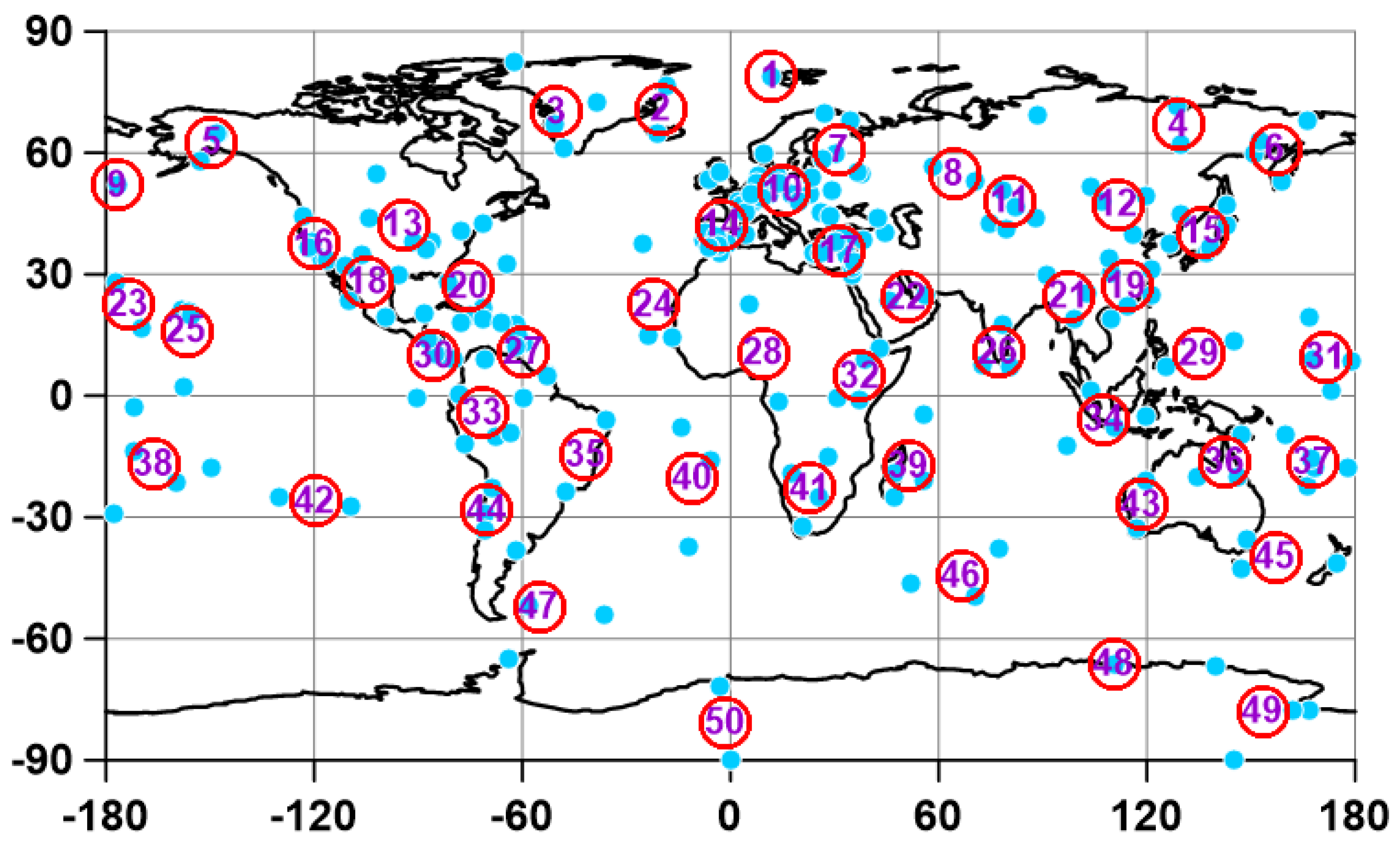
is calculated daily as a median of the values in the 5 nearest operational stations. Thus, continuous time series are obtained with a time sampling 1 day at 50 reference points.
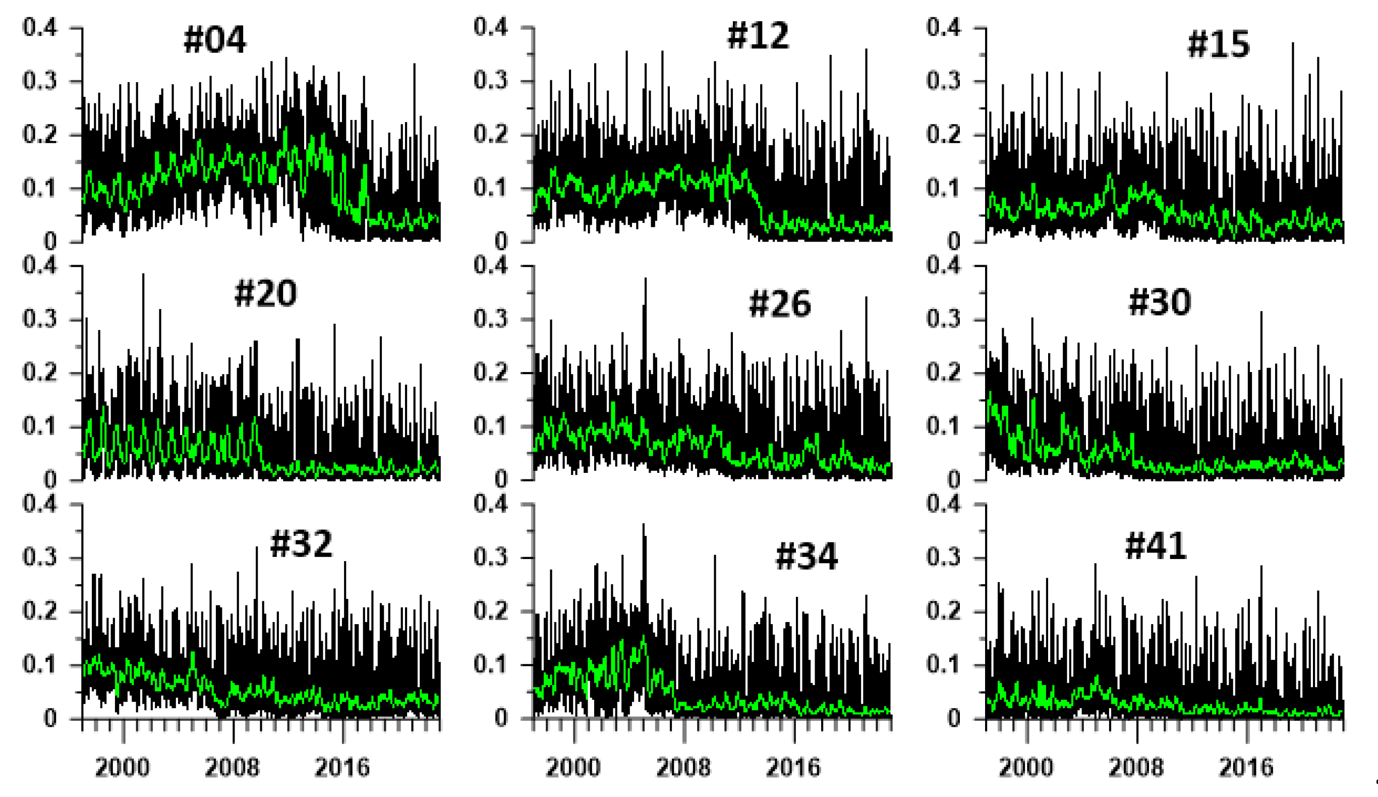
Figure 2 shows the graphs of the index
for 9 reference points (point numbers are indicated next to each graph).
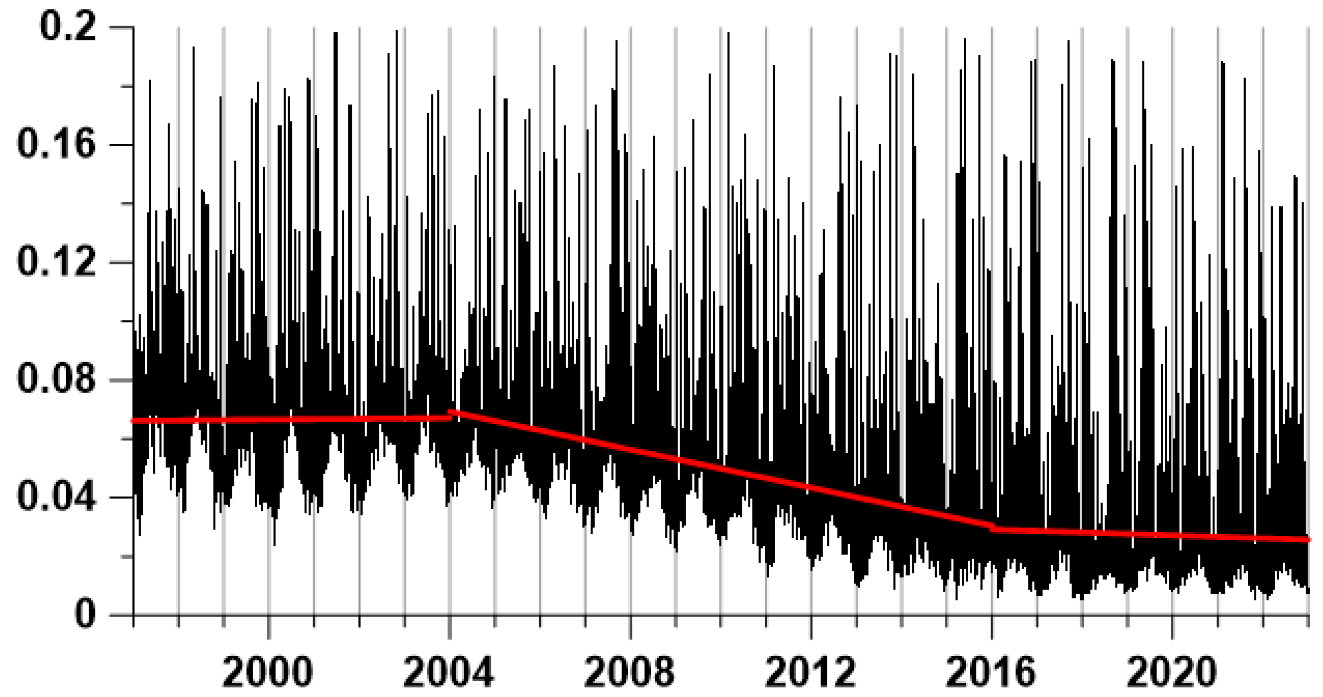
Figure 3 shows a graph of average daily values of index
calculated for all 50 reference points. The red lines represent the linear trends of the average values calculated for the time fragments 1997-2003, 2004-2015 and 2016-2022. The boundaries of time fragments are chosen so that the continuity of the broken line of the union of linear trends is approximately observed. For time intervals 1997-2003 and 2016-2022 linear trends coincide with the average values and it can be seen that during the intermediate time interval 2004-2015 there has been a significant decrease in the global average
. According to the results published in articles [
15,
17,
18], a decrease in the average value of the index
, which is a sign of simplification of the statistical structure of noise (approximation of its properties to the properties of white noise), is associated with an increase in seismic hazard. Thus, the graph of average values in
Figure 3 can be interpreted as a transition to a higher level of global seismic hazard during 2004-2015.
4. Probability densities of extreme values of seismic noise properties
Further analysis of the properties of seismic noise will be based on the identification of regions that are characterized by the most frequent occurrence of extreme values of certain seismic noise statistics. To do this, it is necessary to estimate the probability densities of the distribution over the space of extreme values by their values in the network of reference points. Denote by coordinates of the reference points. Let be the values of any property of the noise at the reference point with the number . We will be interested in maps of the distribution of probability densities of extreme values (minimums or maxima) of values over the Earth's surface. To construct such maps, consider a regular grid of 50 nodes in latitude and 100 nodes in longitude covering the entire earth's surface. Next, maps will be built for various seismic noise statistics , the values of which will be estimated in time windows of various lengths. For each such window, we define the time index , which corresponds to its right end. For each time index , find the reference point with the number , at which the extremum of one or another property is realized, and let be the coordinate of the reference point with the number .
Let
be the distance between the points
and coordinates of the nodes of the regular grid
. Then the value of the probability density of extreme values of the quantity
at the node
of the regular grid can be calculated according to Gaussian distribution:
Here
is the distance, which corresponds to an arc of 15 angular degrees, which is approximately equal to 1700 km, and
is a divisor that provides the normalization condition so that the numerical integral of function (3) over the Earth’s surface is equal to 1. Formula (3) gives "elementary map" of the probability density of the property
extrema distribution for each current window with a time index
. This makes it possible to calculate the average probability density for a given time interval from
to
:
where
is the number of time windows labeled from
to
.
Another way to estimate the variability of the probability density of extreme properties of seismic noise is to construct histograms of the distribution of numbers of control points, in which the statistics extrema are realized. The construction of such histograms in a moving time window, the length of which should include a sufficiently large number of initial time windows within which the noise properties are estimated, makes it possible to determine the reference points at which the minima or maxima of the seismic noise properties are realized most often.
This method has the disadvantage that it does not give a direct distribution of the places of the most probable realization of the noise property extrema in the form of a geographical map, although each reference point has geographical coordinates. On the other hand, this method makes it possible to compactly visualize the temporal dynamics, in particular, to determine the time intervals when the places of concentration of extreme values of the noise statistics change sharply. To solve a similar problem of visualizing temporal dynamics using averaged probability densities (4), one would have to build a laborious long sequence of maps for time fragments consisting of the same number of time windows.
Therefore, in the future, the probability densities of extreme values of noise properties will be presented simultaneously in 2 forms: as averaged densities according to formula (4) for two time intervals, before and after 2011, and as a temporal histogram of the distribution of numbers of reference points in which extremes are realized . In this case, the number of base intervals (bins) of histograms is taken equal to the number of reference points, that is, 50, which makes it possible to visualize the dynamics of the emergence and disappearance of bursts of the probability of extreme values at each reference point.
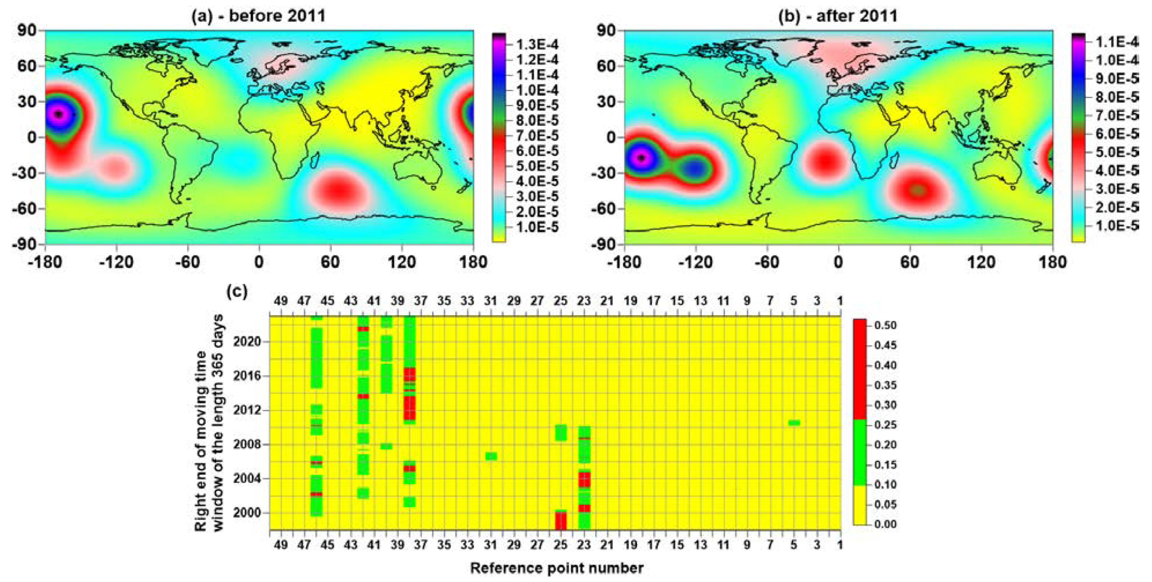
Figure 4(a, b) show maps of distribution of of the minimum values of the DJ index, calculated by formulas (3-4) for windows with time stamps before and after 2011. The choice of 2011 as a boundary time mark is connected, as will be seen from the following presentation, with the fact that the correlation properties of seismic noise changed dramatically after 2 mega-earthquakes: February 27, 2010,
M=8.8 in Chile and March 11, 2011,
M=9.1 in Japan. Previously, this change was already detected in [
3,
18]. Increased attention to the areas where the minimum values
are most often realized, as was already written when discussing
Figure 3, is due to the fact that an increase in seismic hazard is associated with a simplification of the statistical noise structure and a decrease in
. For regions that are quite densely covered with seismic networks, for example, for Japan, this property of statistics
makes it possible to estimate the location of a possible strong earthquake [
17].
However, the global network of seismic stations is sparse and therefore the selection of places where the probability of occurrence of small values is increased does not necessarily coincide with the known places of occurrence of strong earthquakes. On
Figure 4(a, b) the maxima of the probability density distribution of the minimum values
are located in the vicinity of reference points with numbers 23, 25 and 37, 38 in the western part of the Pacific Ocean, where the epicenters of strong earthquakes and volcanic manifestations are really concentrated, including the largest volcanic eruption Hunga Tonga-Hunga Ha'apai January 15, 2022 [
21]. Note that in
Figure 4(c), which shows a diagram of the change in the histogram of the numbers of reference points, in which the minimum value
was realized, one can see the switching of the histogram maximum from the reference point number 23 to the reference point number 38 just after 2011. As for the concentration of probabilities of minimum values
in the vicinity of reference points with number 46 in the southern Indian Ocean (in the vicinity of Kerguelen Island) and in the vicinity of point 40 (Saint Helena) in the Atlantic Ocean after 2011, these features can be associated with mantle plume activation regime [
22].
5. Estimation of Spatial Long-Range Correlations of Seismic Noise Properties
The simplification of the statistical structure of seismic noise manifests itself in a decrease in the average value of the index
(
Figure 3), and is also reflected in an increase in entropy (1) and a decrease in the width of the multi-fractal singularity spectrum support width (“loss of multifractality”). These changes in noise properties are indicators of the transition of a seismically active region (including the whole world) to a critical state [
3,
17].
Another indication of an increase in seismic hazard is an increase in the average correlation as well as the radius of strong correlations between noise properties in different parts of the system. In order to find out how the spatial scale of correlations changes with time, for each reference point we calculate the correlation coefficient between the index
values at this point and at all other reference points. We will perform these calculations in a sliding time window 365 days long with a shift of 3 days. Next, for each reference point, we calculate the average value of the correlation coefficient with the values of
at all other reference points. Since the result of calculating such an average value depends on the time window, we will get graphs of changes in average correlations for all reference points.
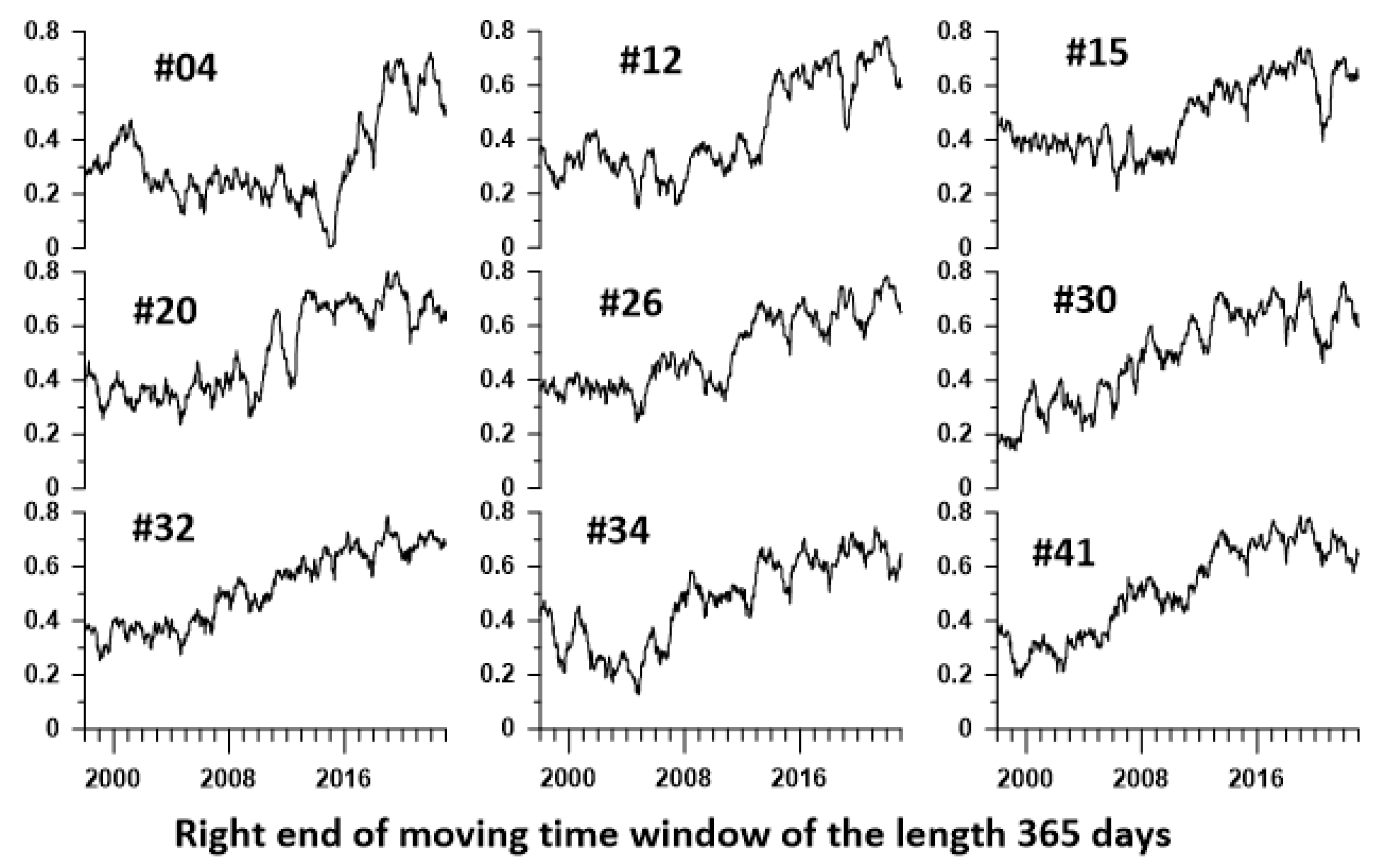
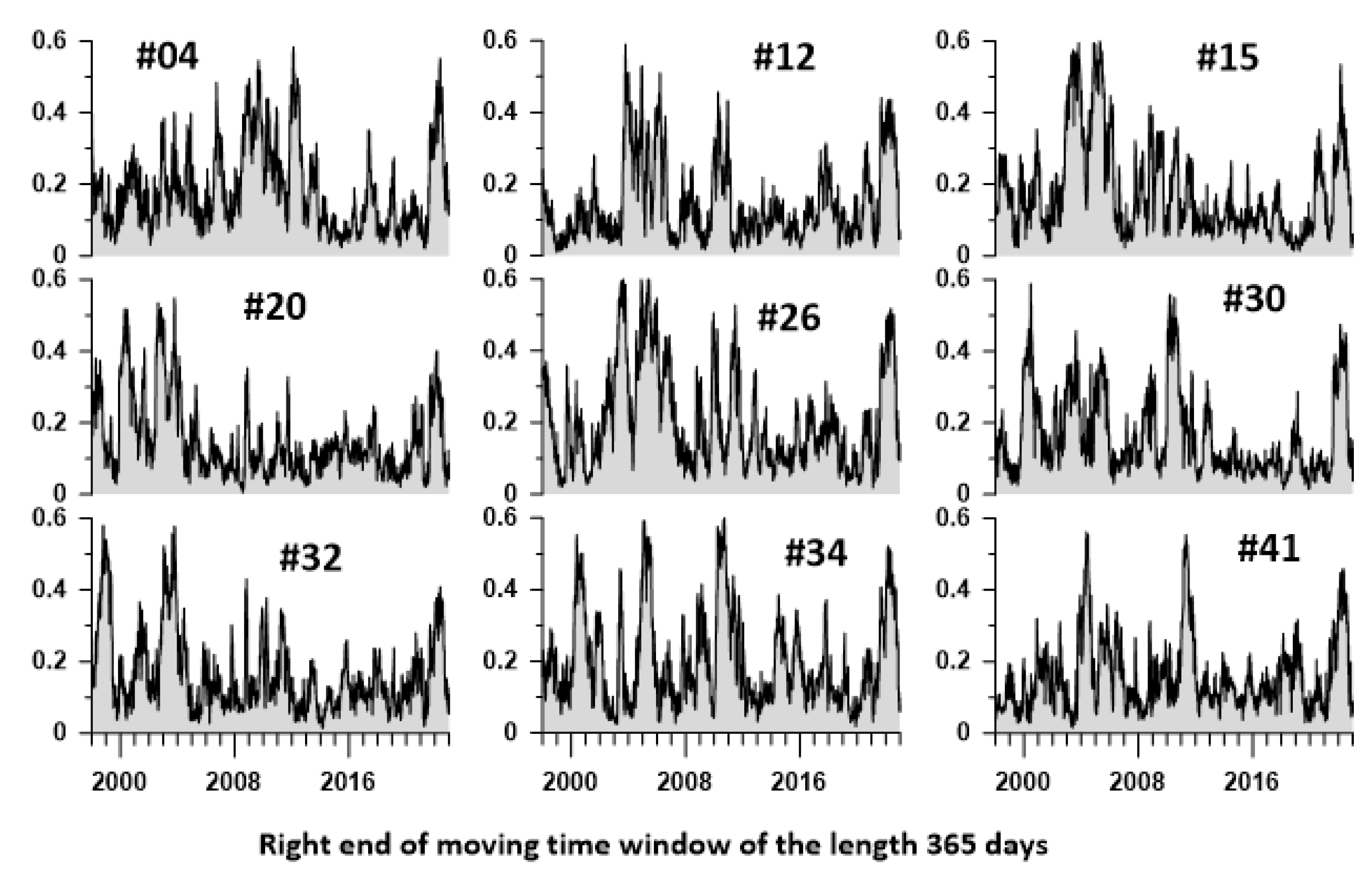
Figure 5 shows examples of graphs of changes in correlations for 9 reference points.
From the graphs in
Figure 5, a general trend towards an increase in the average correlations for each reference point is noticeable. As a result of averaging all graphs of the type shown in
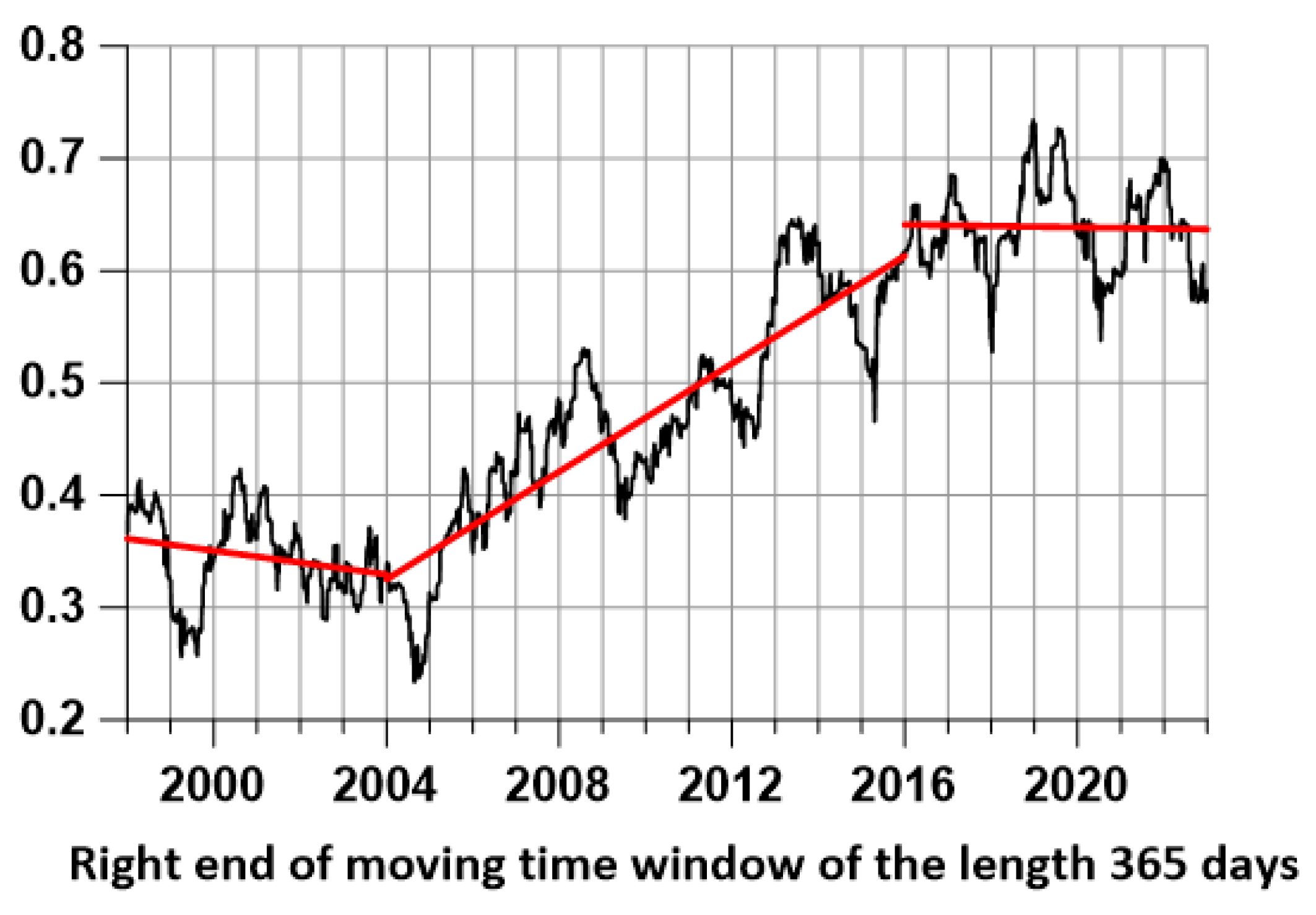
Figure 5 for all 50 reference points, we obtain a general graph of average correlations shown in
Figure 6.
It can be noticed from the graphs in
Figure 6, the time interval 2004-2016, in which the index
decreases (
Figure 3), corresponds to an increase in average correlations between the properties of noise at various reference points and there is a transition from small correlations before 2004 to fairly large correlations after 2016.
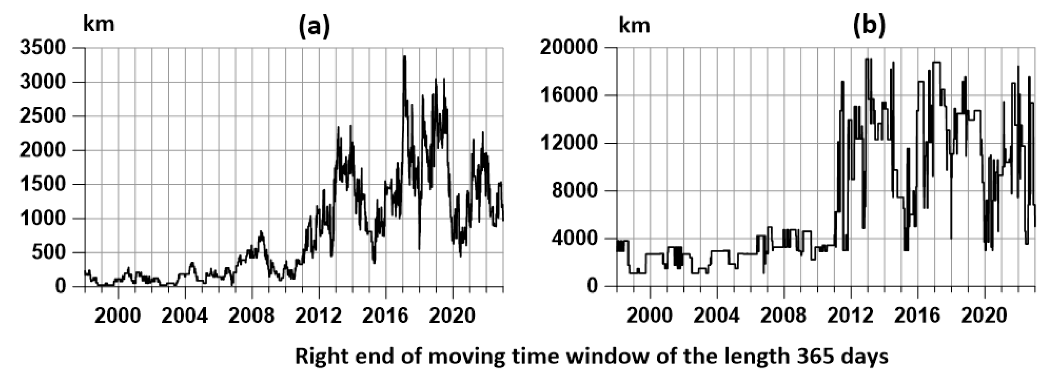
In order to assess the scale of strong correlations between seismic noise properties, for each reference point we define another point that has a maximum correlation with this point, provided that this maximum exceeds the threshold of 0.8, and calculate the distance between these points.
Figure 7 shows the graphs of the change in the average and maximum values of the distances between points for which the correlation maxima exceed 0.8.
It can be seen from the graph in
Figure 7(b) that after 2011 there was a sharp increase in the maximum distance at which strong maximum correlations occur. Thus, the growth of average correlations, which is visible in
Figure 6, is supplemented by an explosive growth of the maximum scale of strong correlations.
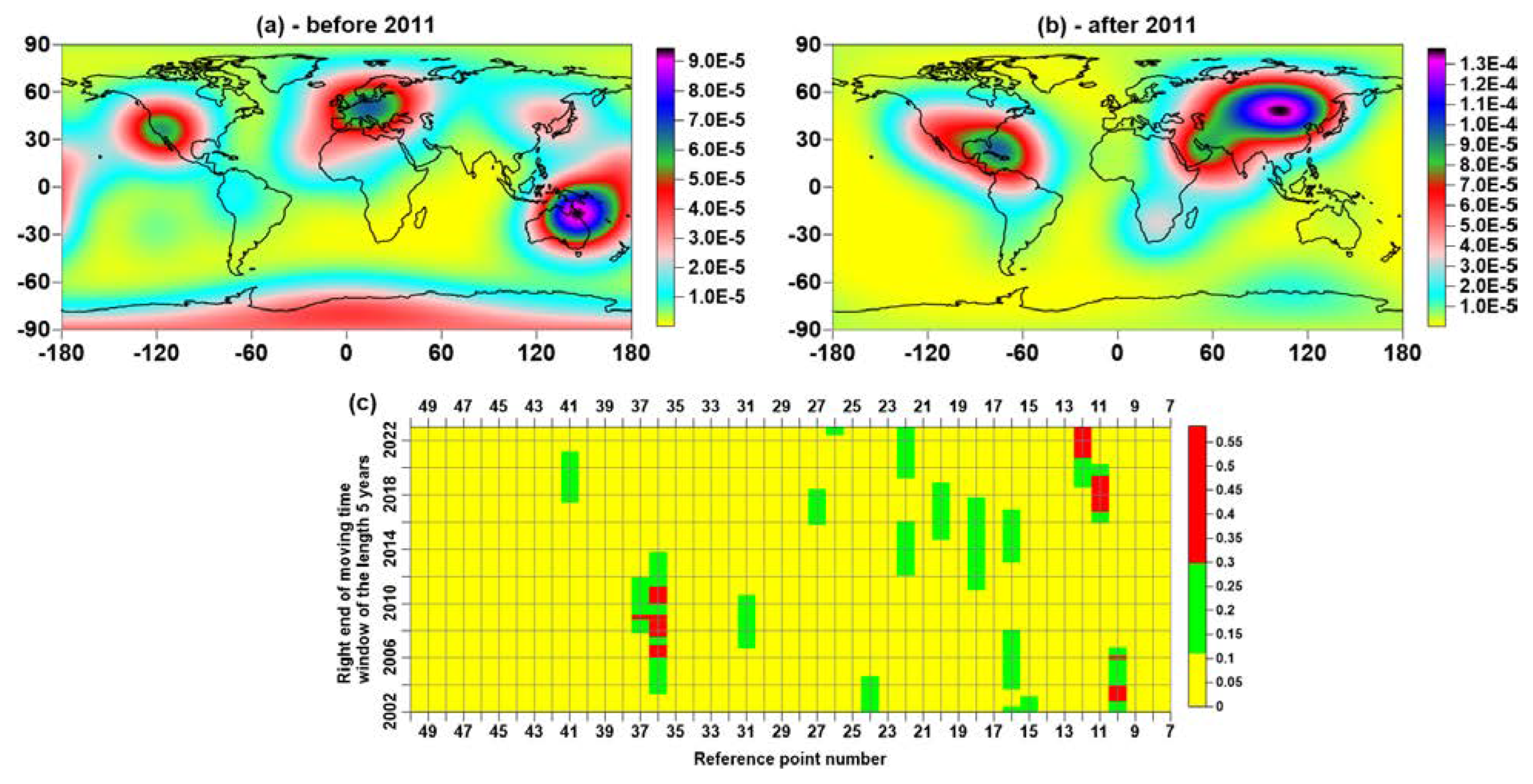
It is of interest to identify those reference points in the vicinity of which strong correlations most often occur. As before, for this purpose we use estimates (3-4) of the probability density of the distribution over space of the maximum correlation values for the time intervals before and after 2011, as well as the distribution histograms of the numbers of control points in which the maximum correlation values occurred.
To select the length of the time window for calculating histograms, we recall that the correlation coefficients between the values at each reference point with the values of the DJ index at other reference points are calculated in windows of 365 days with a shift of 3 days. Let us choose the length of the window for calculating histograms so that the dimensional length of the window is equal to 5 years. It is easy to calculate that this length will be 488 values of "short" time windows with a length of 365 days with an offset of 3 days. In this case, the histogram is calculated in a window of length 365+3⋅(488-1)=1826 days, which is approximately equal to 5 years, given that every 4th year is a leap year. As for the number of base intervals (bins) of histograms, in this case there will be not 50, as in
Figure 4(c), but 44, since for reference points with numbers 1-6 there are no realizations of correlation maxima.
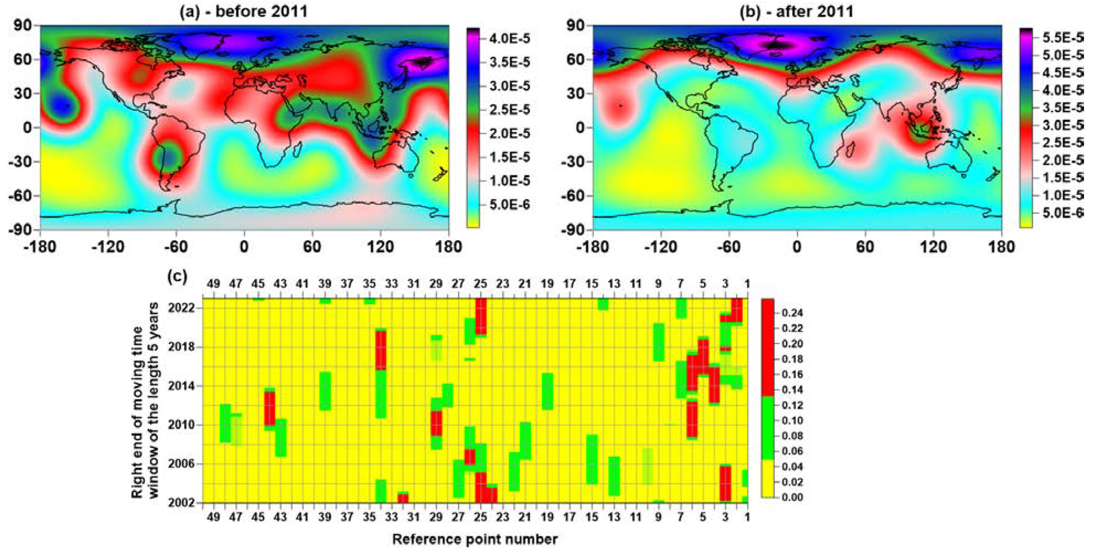
Estimates of the position and temporal dynamics of places with an increased probability of maximum correlations are presented in
Figure 8. Comparison of
Figure 8(a) and 8(b) shows that the places of concentration of maximum correlations have changed significantly since 2011. In particular, there has been a rapid shift of such a center from the Southwest Pacific to Central Eurasia, which can be seen in the histogram diagram in
Figure 8(c).
6. Seismic Noise Response to the Irregularity of the Earth's Rotation
The connection between irregular rotation of the Earth and seismicity was investigated in [
23]. An influence of strong earthquakes on the Earth’s rotation was studied in [
25].
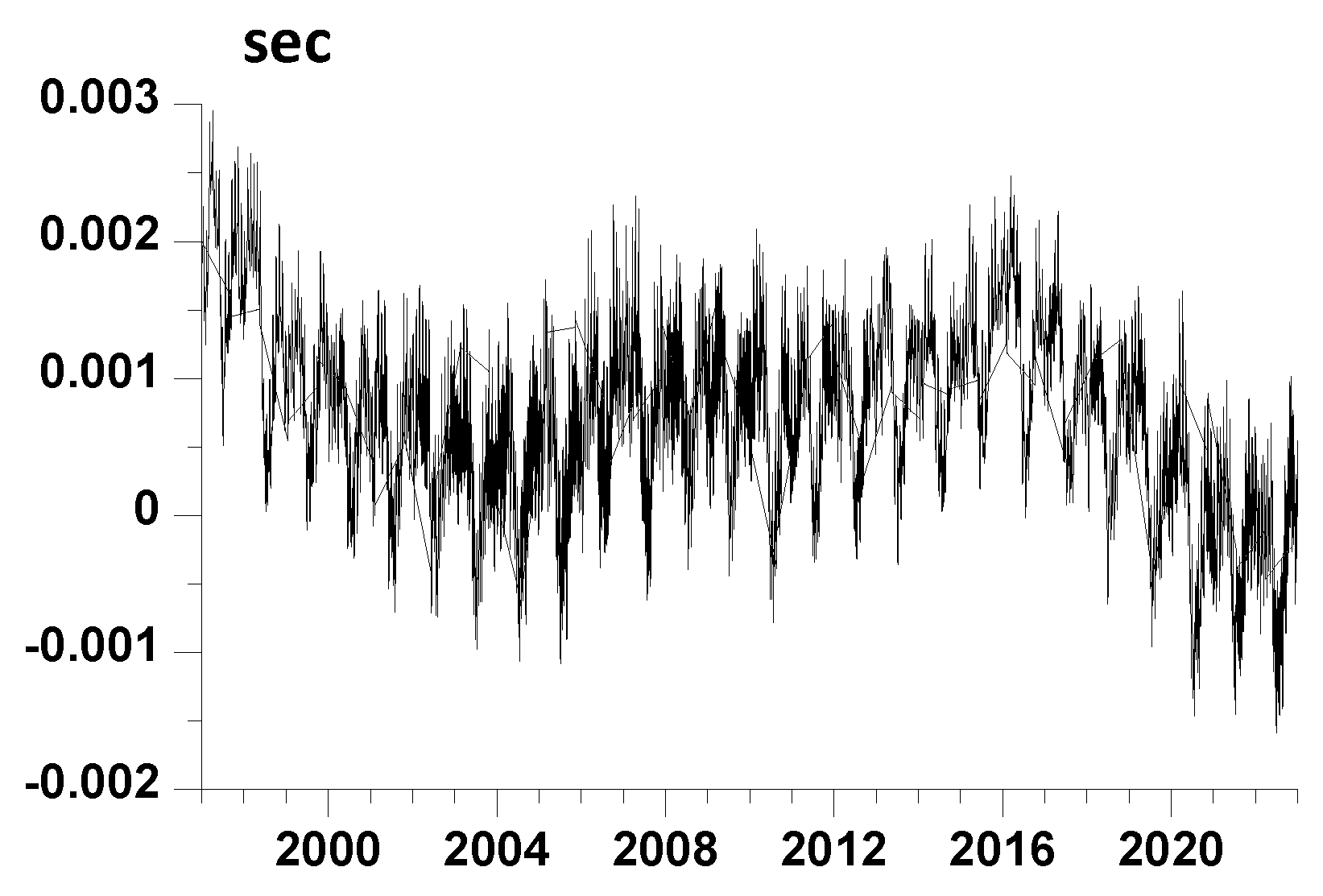
Figure 9 shows a graph of the time series of the length of the day for the time interval 1997-2022.
Further, the LOD time series is used as a kind of "probing signal" for the properties of the seismic process [
3,
15,
16,
17,
18]. To study the relationship between the properties of the seismic process and the irregularity of the Earth's rotation, the squared coherences maxima between the LOD and the properties of seismic noise at each reference point were estimated. The coherences were estimated in moving time windows of 365 days with a shift of 3 days using a vector (two-dimensional) 5th order autoregressive model [
15,
16,
17,
18]. In what follows, these maximum coherences will be referred to as the seismic noise
responses to the LOD.
Figure 8 shows examples of LOD response graphs at 9 reference points.
We define the integrated response of the global seismic to the LOD as the average of the responses of the type shown in
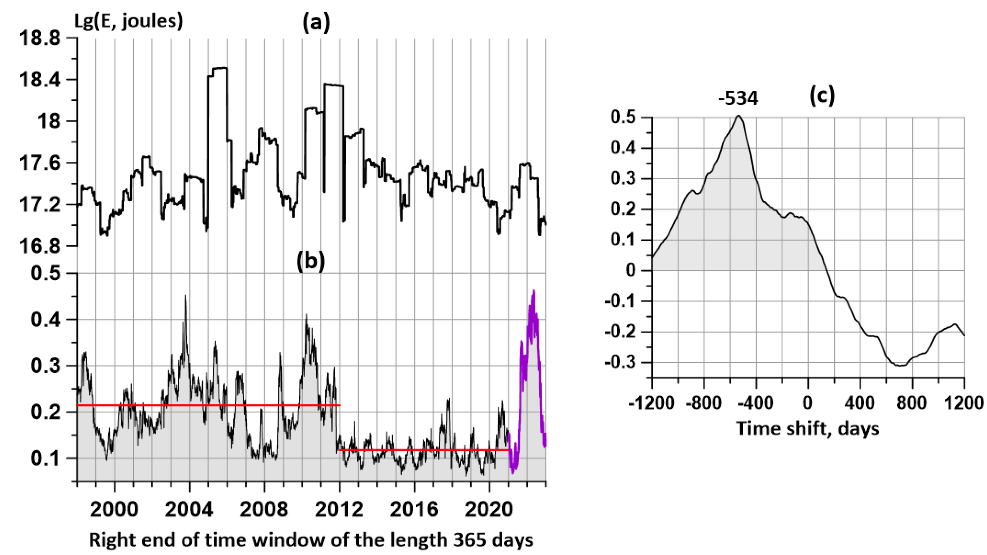
Figure 10 from all 50 reference points. Let us compare the behavior of the average response to LOD with the amount of released seismic energy. To do this, we calculate the logarithm of the released energy as a result of all earthquakes in a moving time window 365 days long with a shift of 3 days. On
Figure 11 (a, b) there are graphs of the logarithm of the released energy and the average response to the LOD. It is visually noticeable that bursts of the average maximum coherence in
Figure 11(b) precede the energy spikes in
Figure 11(a). In order to quantitatively describe this delay, we calculate the correlation function between the curves in
Figure 11(a, b). The graph of this correlation function for time shifts of ±1200 days is shown in
Figure 11(c).
The estimate of the correlation function in
Figure 11(c) between the logarithm of the released seismic energy in
Figure 11(a) and the average response of seismic noise to LOD has a significant asymmetry and is shifted to the region of negative time shifts, which corresponds to the coherence maxima being ahead of the maxima of seismic energy emissions. The correlation maximum corresponds to a negative time shift of 534 days. This estimate of cross-correlations gives a foundation to propose that the burst shown in
Figure 11(b) by the magenta line may precede a major earthquake with an average delay of 1.5 years.
The curve in
Figure 11(b) can be split into 3 sections. The first 2 intervals with time marks of the right ends of windows before and after 2012 differ significantly from each other by their mean values presented by red lines.
The third time interval in
Figure 11(b) is presented by the magenta line and refers to the processing of the most recent data which correspond to right-hand end windows after 2021 i.e. referring to the time span of 2020-2022. Identification of a short 3rd segment based on the results of data processing in 2021-2022 due to an unusually large spike in the response of noise properties to LOD. The maximum value of the response in
Figure 11(b) is reached at the time corresponding to the date 2022.05.09. The "naive" forecast, which consists in the fact that 534 days are added to this date, gives the most probable date for the future strong event on 2023.10.24. A more realistic prediction would be to blur this date with some uncertainty interval. However, it is not yet possible to give such an interval due to the small history of using the seismic noise response to LOD as a predictor.
Similarly to how it was done to identify the places of concentration of maxima of spatial correlations of seismic noise in
Figure 8, we can search for places where the maximum response of seismic noise properties to the uneven rotation of the Earth is most likely. The results of such a search are shown in
Figure 12. Comparison of
Figure 12(a) and 12(b) shows that the maximum response to LOD is concentrated in the subarctic regions.
In addition to the issue of synchronization of seismic noise properties, which are reflected in the graphs in
Figure 5,
Figure 6 and
Figure 7, we also study the synchronization of seismic noise responses to the irregularity of the Earth's rotation. Previously, this issue was considered for the synchronization of seismic noise responses to LODs in Japan and California [
16].
For each reference point, we estimate the correlation of the response at this point with the responses at all other points. It should be taken into account that the correlated responses themselves were calculated in sliding time windows of 365 days with a shift of 3 days. These were "short" time windows. Now we need to take a certain number of consecutive "short" windows and form a "long window" from them, such that it contains a sufficiently large number of noise response estimates to LOD in "short" time windows. Next, 250 adjacent "short" windows were selected to form a "long" window. Correlation coefficients between responses to LOD at various reference points were calculated in a sliding "long" window with a shift of 1, that is, in a time window with a length of 365+3⋅ (250-1)=1112 days, which is approximately 3 years. A shift of 1 count means a real shift of 3 days.
The goal of such calculations for each reference point is the average correlations of responses over all other reference points. As a result of such averaging, 50 dependences of the same type as shown in
Figure 5 will be obtained. In order to obtain an integrated measure of the correlation of global noise responses to LOD, the average dependences for all reference points should be averaged secondary. As a result, we get the graph shown in
Figure 13.
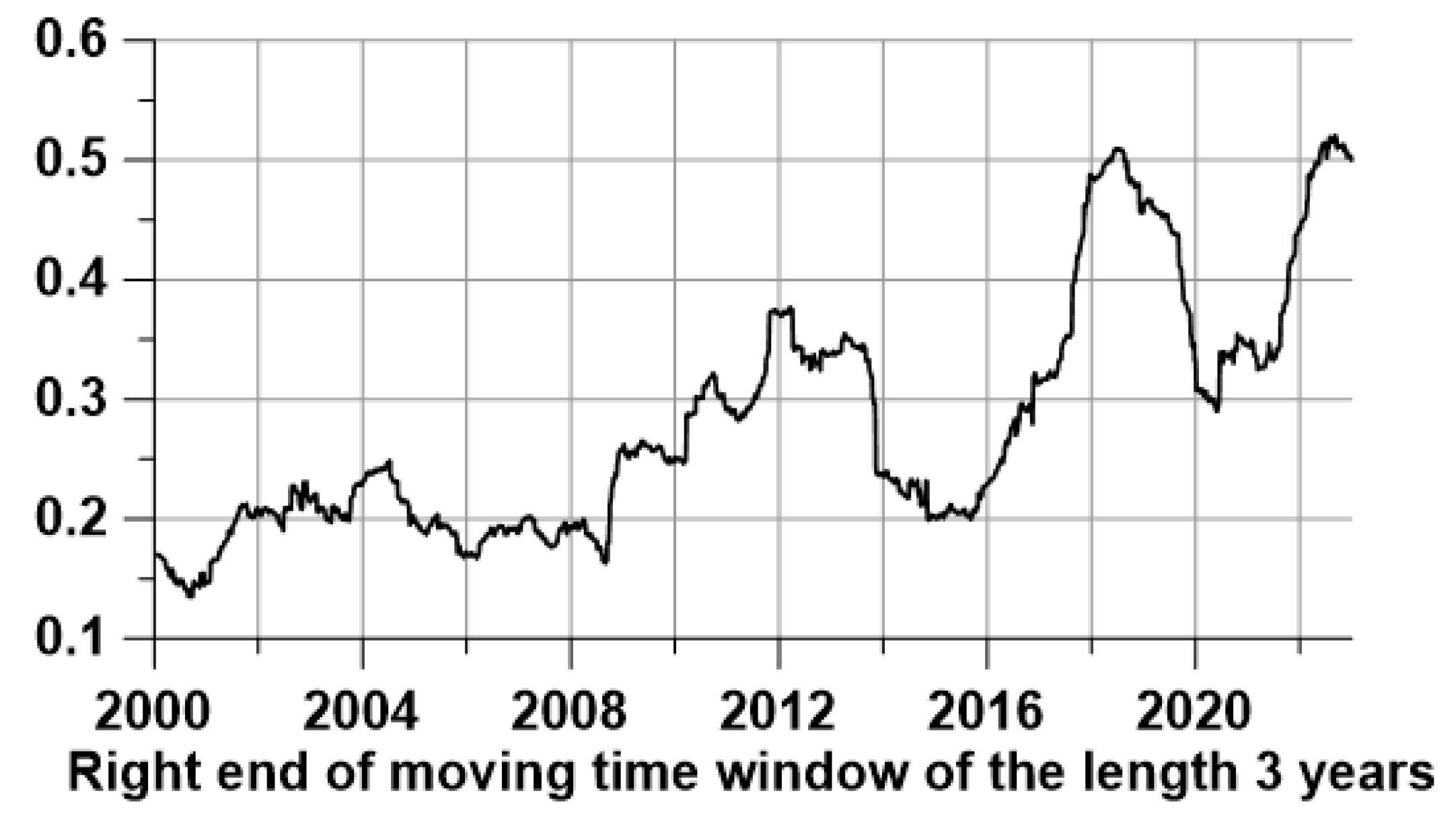
Figure 13 shows the change in time of the measure of synchronization of the response of seismic noise to the irregularity of the Earth's rotation. This graph also shows the growth of correlations, similar to the growth of the initial correlations in
Figure 6.
Figure 1.
Positions of 229 broadband seismic stations (blue circles) and a network of 50 reference points (numbered red circles).
Figure 1.
Positions of 229 broadband seismic stations (blue circles) and a network of 50 reference points (numbered red circles).
Figure 2.
Graphs of daily index values for 9 reference points. The green lines represent the moving averages in a 57 day window.
Figure 2.
Graphs of daily index values for 9 reference points. The green lines represent the moving averages in a 57 day window.
Figure 3.
Graph of the average daily values of the DJ index for all 50 reference points. Red lines present linear trends for 3 time intervals: 1997-2003, 2004-2015 and 2016-2022.
Figure 3.
Graph of the average daily values of the DJ index for all 50 reference points. Red lines present linear trends for 3 time intervals: 1997-2003, 2004-2015 and 2016-2022.
Figure 4.
(a) and (b) are the probability densities of the distribution of the minimum values of the seismic noise index in a network of 50 control points before and after 2011; (c) - histogram of numbers of control points, in which the minimum values of the index were realized in a moving time window 365 days long.
Figure 5.
Graphs of the average correlation coefficients of the index for 9 data points with values at other data points in a moving time window of 365 days with mutual shift 3 days.
Figure 5.
Graphs of the average correlation coefficients of the index for 9 data points with values at other data points in a moving time window of 365 days with mutual shift 3 days.
Figure 6.
The average correlation coefficient between the values of the DJ-index at each control point with the values at other points. Red lines show linear trends for 3 intervals of time marks of the right ends of windows with a length of 365 days: 1998-2004, 2004-2016 and 2016-2023. On the last time fragment, the linear trend coincides with the average value.
Figure 7.
(a) - the average distance between the reference points for which the maxima of correlations between the values of the DJ-index of seismic noise exceeded the threshold of 0.8; (b) - the maximum distance between the reference points with the maximum correlation coefficient above the threshold of 0.8.
Figure 8.
(a) and (b) are the probability densities of the correlation maxima between for index values at each reference point with index values at other reference points before and after 2011; (c) - a histogram of the numbers of reference points, in which the correlation maxima for values of at each reference point with the values at other points in a moving time window of 5 years were realized.
Figure 10.
Plots of maximum squared coherence between index and LOD in a moving time window of 365 days with mutual shift 3 days for 9 reference points.
Figure 10.
Plots of maximum squared coherence between index and LOD in a moving time window of 365 days with mutual shift 3 days for 9 reference points.
Figure 11.
(a) is the logarithm of the released seismic energy (in joules) in a sequence of time intervals 365 days long, taken with an offset of 3 days; (b) - average values of maximum coherences between LOD and daily DJ-index values at 50 reference points; (c) is the correlation function between the logarithm of the released seismic energy and the average value of the maximum coherence between the LOD and the seismic noise DJ index at 50 reference points.
Figure 12.
(a) and (b) are the probability densities of the seismic noise index response maxima to LOD before and after 2011; (c) - histogram of numbers of reference points, in which the maximum values of the index response to LOD were realized in a sliding time window of 5 years
Figure 12.
(a) and (b) are the probability densities of the seismic noise index response maxima to LOD before and after 2011; (c) - histogram of numbers of reference points, in which the maximum values of the index response to LOD were realized in a sliding time window of 5 years
Figure 13.
The average value of the correlation coefficients between the seismic noise index responses per LOD for each of the 50 control points with responses at other points.
Figure 13.
The average value of the correlation coefficients between the seismic noise index responses per LOD for each of the 50 control points with responses at other points.
