Assessing the Likelihood of Failure Due to Stem Decay Using Different Assessment Techniques

Arborists commonly investigate the extent of stem decay to assess the likelihood of stem failure when conducting tree risk assessments. Studies have shown that (i) arborists can sometimes judge the extent of internal decay based on external signs; (ii) sophisticated tools can reliably illustrate the extent of internal decay; and (iii) assessing components of tree risk can be highly subjective. We recruited 18 experienced tree risk assessors who held the International Society of Arboriculture’s Tree Risk Assessment Qualification (TRAQ) to assess the likelihood of stem failure due to decay after each of 5 consecutive assessments on 30 individuals of 2 genera. Five assessment techniques, in stepwise order, were 1) visual, 2) sounding the trunk with a mallet, 3) viewing a scaled diagram of the cross-section that revealed sound and decayed wood ascertained from resistance drilling, 4) viewing sonic and electrical resistance tomograms, and 5) consulting with a peer. For each technique, assessors assigned two or more likelihood of failure ratings (LoFRs) for at least 83% of trees, which were proportionally greatest after assessors viewed tomograms; the proportions did not differ among the other four assessment techniques. Covariates that influenced the distribution of LoFRs included percent of the cross-section that was decayed, and assessors’ experience using resistance drilling devices and tomography in regular practice. Practitioners should be aware that disagreement on the likelihood of tree failure exists even among experienced arborists.

Keywords:

Subject: Biology and Life Sciences - Forestry

1. Introduction

Urban forests and greenspaces are increasingly considered an important priority for improving the sustainability, resilience, and livability of the urban landscape [1]. Trees in the urban forest provide many benefits such as air pollution reduction [2], storm water runoff attenuation [3], carbon sequestration [4], and building energy conservation [5]. Benefits generally increase as the size of trees increase [6], but as trees mature they are more likely to develop decay that increases their likelihood of failure [7]. In built environments, tree failures can result in fatalities [8], power outages [9], and catastrophic fires [10]; and damage from failures is associated with higher costs [11] and legal liability [12].

Arborists have assessed tree risk for many years. Recent revisions have brought the process into better alignment with risk assessment practices used in other disciplines. The current U.S. standard considers 1) the likelihood of a tree failure, 2) the likelihood of impact of a tree or tree part on a target and 3) the severity of the consequence if impact were to occur. Arborists assign one of four ratings to likelihood of failure (improbable, possible, probable, imminent) that are defined as follows: [13]:

Improbable: The tree or tree part is not likely to fail during normal weather conditions and may not fail in extreme weather conditions within the specified time frame.
Possible: Failure may be expected in extreme weather conditions, but it is unlikely during normal weather conditions within the specified time frame.
Probable: Failure may be expected under normal weather conditions within the specified time frame.
Imminent: Failure has started or is most likely to occur in the near future, even if there is no significant wind or increased load. This is a rare occurrence for a risk assessor to encounter and may require immediate action to protect people from harm. The imminent category overrides the stated time frame.

Decay is a common defect that is often associated with tree failure [7,14,15]. Decay reduces load-bearing capacity by reducing wood strength and, if wood components are completely digested, by creating voids that reduce cross-sectional area. Many tools and techniques to detect and assess the extent of decay have been developed. Some are simple (e.g., sounding the stem with a mallet); others are sophisticated (e.g., resistance drills and tomography) [16]. Many studies have investigated how well decay detection tools and techniques work [17,18,19,20,21,22,23,24].

Despite advancements in decay detection tools and techniques, many aspects of risk assessment remain uncertain because of the lack of knowledge about how trees grow and fail. Uncertainty may also be exacerbated by assessor bias, including an assessor’s personal risk tolerance [25]. Cognitive studies on human risk perception attribute an individual’s attitude towards risk to personal experiences [26,27], personal fears [28], and biases shared by communities [29]. An assessor’s training also influences ratings: trained professionals tended to return lower likelihood of failure ratings (LoFRs) than those without training [25,30].

Our objectives for this study were as follows:

to determine whether more detailed information about the extent of trunk decay influenced experienced assessors’ LoFRs and, if so,
to identify factors related to assessors and trees that explained the influence.

2. Materials and Methods

The study took place on the campus of the University of Massachusetts in Amherst, Mass., USA (USDA Hardiness Zone 5b). In July 2021, 18 experienced arborists who held the International Society of Arboriculture’s (ISA) Tree Risk Assessment Qualification (TRAQ) (among other credentials) assessed the likelihood of stem failure due to decay of 30 trees using 5 (basic and advanced) assessment techniques.

We selected trees for the field assessment based on practical considerations. The first was the availability of sonic and electrical resistance (ER) tomograms taken of the trunk taken within 2 m of the ground. Tomograms had been previously obtained using a PiCUS Sonic Tomograph 3, a TreeTronic 3 for ERT, and the Caliper 3 Geometry Measurement System (Argus Electronic GMBH, Rostock, Germany) following the methods of [23]. A second consideration was variation in compartmentalization response: weak (Pinus) and strong (Quercus). Finally, only (i) larger individuals (> 50 cm stem diameter measured 1.4 m above ground—“DBH”) and (ii) individuals that were close enough to one another that they could be grouped by location were selected. In the latter case, we selected individuals in six discrete clusters around the campus. We selected clusters of individuals for two reasons: (i) it included a variety of landscape settings (open space or near infrastructure such as roads, buildings, and parking lots); and (ii) it limited travel time to maximize the number of individuals that could be assessed in the two days when assessors visited campus. Prior to conducting the study, we pre-tested the methods and determined an efficient route to assess as many trees as possible in two days.

We recruited assessors from our professional networks, inviting only experienced assessors who (i) held the TRAQ credential, (ii) regularly performed risk assessments as part of their professional practice, and (iii) were familiar with advanced decay detection techniques such as resistance drilling and tomography. We offered continuing education units to assessors, but neither financial compensation nor reimbursement of travel expenses.

Before assessors arrived on campus in July 2020 to participate in the study, we used a Resistograph® F500-S (IML North America, Moultonborough, N.H., USA) to determine the thickness of sound wood (t) at between three and six locations spaced at approximately even intervals around the stem circumference and at the same height as the tomogram. For each location, we computed the t/R ratio, where R is trunk radius [31]. We attached flagging to the stem to indicate the locations of the tomography and Resistograph measurements (Figure 1).

We provided each assessor a binder that included a sheet for each tree. The sheet contained the following information: genus and species, DBH, height, the Resistograph output (Figure 2), and the sonic and ERT tomograms (Figure 3). Output from the Resistograph included a scaled diagram of the cross-section of the stem and lines indicating where drillings were made, the height and stem diameter where the drillings were made, the mean t value, and a table of all t/R values. The tomograms included the percentages of cross-sectional area that were sound or decayed. The decayed proportion of the cross-section was computed automatically from the combined areas of blue and purple in the sonic tomogram. Since we used the default settings (SoT1 calculation option and minimum velocity established at 50%), the resulting tomogram depicts the greatest possible area of decay in comparison to those generated using SoT2 and an expanded color space to view the minimum percent velocities. But the computed proportion of decayed wood indicated at the top of the tomogram assessors viewed during the study (e.g., Figure 3) did not include areas of intermediate velocities. We explained this to assessors prior to the field study. After the field study, we computed the loss in section modulus due to decay (Z_LOSS) from each sonic tomogram following the method of [32].

We instructed assessors to assign a rating of the likelihood of stem failure due to decay (“LoFR”) within 2 m of the ground and reminded them not to assess likelihood of failure of other parts of the tree. We used LoFRs from [13] and provided assessors with the definitions (listed in the Introduction). We instructed assessors to assign their LoFR based on a timeframe of three years.

Assessors performed five consecutive assessments of the LoFR. In order, assessments were as follows:

visual assessment of the tree and its surroundings;
sounding the trunk with a plastic mallet;
viewing the Resistograph output (Figure 2);
viewing the tomograms (Figure 3);
consulting with a randomly assigned assessor.

Assessment techniques (a) and (b) are part of a Level 2 (“basic”) risk assessment [13]. Assessment techniques (c) and (d) are more sophisticated techniques to assess the amount and location (i.e., the “extent”) of decay and part of a Level 3 (“advanced”) risk assessment [13]. For odd-numbered trees, assessors viewed the resistance drilling output (c) before the viewing the tomogram (d); for even-numbered trees, assessors viewed the tomogram first. Consulting with a peer is not explicitly recommended in common professional guidelines [13,33]. Within each cluster of trees, assessors were randomly paired and inspected individual trees at their own pace.

After each of the five assessments [(a) – (e)] on a tree, assessors completed a survey to indicate their LoFR and describe the factor(s) (e.g., species, decay severity, tree size, exposure, lean, crown, etc.) that most influenced their LoFR, and if the additional information gained in the assessment technique changed their LoFR.

Assessors also self-reported the following information on the survey: years of experience performing tree risk assessments; number of trees assessed annually; relevant credentials in addition to TRAQ; and how frequently they used assessment techniques (b), (c), and (d) as part of their professional practice.

During the field study, not every assessor completed all five assessments of every tree. As a result, approximately 15% of the expected dataset was missing values. We used multivariate imputation by chained equations [34,35] to impute the most likely value for each missing value to obtain a full dataset prior to OLR analyses.

The university campus is well maintained, and no assessor assigned a LoFR of four (“imminent”) to any tree. Consequently, we coded LoFR ordinally as one (“improbable”), two (“possible”), or three (“probable”) and built ordinal logistic regression (OLR) models to investigate the effect of assessment technique on LoFR. All analyses were performed using the statistical language R, v4.1.2 [36]. In the OLR models, we included covariates describing trees [genus; DBH; percent of cross-sectional area with decay (from tomograms); average sound wood thickness (t) from the Resistograph output; t/R, where R is stem radius; Z_LOSS] and participants (years of experience; frequency of using a mallet, resistance drilling, and tomography when conducting risk assessments). We also included tree and assessor identification as random effects in each OLR model. We built models with the “clmm” function from the “Ordinal” package by iteratively adding covariates as single effects or interactions with the main effect of assessment technique [37]. Since the order of assessments differed between even- (viewed tomogram before Resistograph output) and odd-numbered (viewed Resistograph output before tomogram) trees, the variable “assessment technique” contained ten levels that represented an interaction between the five assessment techniques and even- or odd-numbered trees. We then selected the best model using lowest AICc scores.

In addition to the OLR analyses, we created a contingency table with four rows (one for each of the assessment techniques that followed the initial visual assessment) and two columns (to indicate whether the additional information gained for the assessment technique changed (“Yes”) or did not change (“No”) assessors’ LoFRs). We used a

χ^{2}

test to determine whether the proportion of affirmative and negative responses varied among assessment techniques.

Lastly, we investigated the influence of the random variables in the OLR model (assessor and tree) on LoFR. To investigate the influence of assessors, we evaluated if the consistency in assessor LoFRs changed among the five assessment techniques or four frequency-of-use categories of the tomogram or Resistograph. We quantified LoFR consistency with the “betadisper” function in the “vegan” package, which performed a multivariate test of homogeneity of variances on a Bray-Curtis (rank-based) dissimilarity matrix of the proportional distribution of LoFRs [38]. A multivariate approach was needed to evaluate inconsistencies of LoFRs with a single test.

To investigate the influence of trees between the initial visual assessment and each subsequent assessment technique, we computed the ratio of the weighted mean change in LoFR to the proportion of unchanged LoFRs for each tree. The ratio illustrated the frequency, magnitude, and direction of changes in LoFR from the initial visual assessment. We computed the ratio (

R

) as follows:

Compute the difference in LoFR from the initial visual LoFR:

${{∆ L o F R}_{i j k} = L o F R}_{i j k} - {L o F R}_{v j k}$

where $i$ , $j$ , and $k$ , are indices for the 4 assessment techniques following the initial visual assessment (indicated by the subscript $v$ ), 30 trees, and 18 assessors, respectively.
Compute the proportion of unchanged LoFRs (i.e., $∆ L o F R = 0$ ) for each tree and assessment technique:

$κ_{i j} = \frac{|{∆ L o F R}_{i j} = 0|}{|{∆ L o F R}_{i j}|}$

(2)
Compute the weighted mean change in LoFR:

$\bar{{∆ L o F R}_{i j}} = \frac{\sum_{i j} ({∆ L o F R}_{i j} * ω_{i j})}{|{∆ L o F R}_{i j}|}$

(3)

where $ω$ is a weighting factor of 1 (for LoFRs that changed one level from the initial visual assessment, e.g., from probable to possible or improbable to possible) or 2 (for LoFRs that changed two levels, e.g., from probable to improbable).
For each tree and assessment technique,

$R_{i j} = \frac{\bar{{∆ L o F R}_{i j}}}{κ_{i j}}$

(4)

We thus computed 30 values of

R

for each of the 4 assessment techniques that followed the initial visual assessment. From the resulting distribution of 120 values of

R

, we considered only values in the upper and lower quartiles as having increased and decreased LoFR, respectively. We considered values of

R

within the interquartile range (IQR) as having the same LoFR as the initial visual assessment. In the rest of the paper, we refer to “increased”, “decreased”, or “unchanged” LoFRs rather than values of

R

in upper quartile, lower quartile, and IQR, respectively.

We described the basic assessment techniques as “consistent” if the LoFR assigned in the mallet assessment was unchanged from the initial visual assessment, and “inconsistent” if the LoFR assigned in the mallet assessment was greater or less than the initial visual assessment. We described the advanced assessment techniques as consistent if the change in LoFR from the initial visual assessment was the same for both advanced assessment techniques. We described the advanced assessment techniques as inconsistent if the change in LoFR from the initial visual assessment was not the same for both advanced assessment techniques. With respect to changes in LoFR from the initial visual assessment, we described the effect of the consultation assessment as “confirming” (or not) the basic and advanced assessments. If the LoFR assigned in the mallet and consultation assessments was unchanged from the initial visual assessment, the consultation assessment confirmed the basic assessment techniques. Similarly, if the LoFR was greater than or less than the initial visual assessment for both advanced assessment techniques and the consultation assessment, the consultation confirmed the advanced assessment techniques.

3. Results

3.1. Assessors

On average, assessors held the TRAQ credential for 6.1 years (3.1 years standard deviation). Some assessors additionally held the following credentials: ISA Board Certified Master Arborist (39%), American Society of Consulting Arborists (ASCA) Registered Consulting Arborist (39%), an advanced degree (M.S., Ph.D.) in arboriculture or a related field (67%). All assessors conducted tree risk assessments as part of their job; the mean years of practice was 14.3 (10.8 years standard deviation) with a mean of 425 trees assessed annually (737 trees standard deviation). Table 1 includes assessors’ responses to inquiries about their level of experience with the techniques and tools used in the study. Nearly all “often” conducted basic visual assessments using a mallet; a majority often or “occasionally” used a resistance recording drill, sonic tomography, or both.

3.2. Trees

Trees were semimature to mature, and large, with proportions typical of open-grown trees (Table 2). Table 2 also includes (i) the stem height at which tomography and Resistograph drilling were conducted, and (ii) the following covariates included in the OLR models for each tree: mean t value, minimum t/R ratio, percent decayed wood in the stem cross-section, and Z_LOSS.

Table 3 includes the fixed effects and interactions of the best OLR model to predict LoFR. Assessment technique influenced the predicted proportions of improbable, possible, and probable LoFRs (Table 3). The proportion of improbable LoFRs was least after assessors viewed tomograms; proportions of improbable, possible, and probable LoFRs were statistically similar among the other four assessment techniques (Figure 4). There were also significant interactions between assessment technique and the following covariates: percentage of decayed wood in the cross-section, mean t, and how often a participant used resistance drilling in professional practice (Table 3).

As the percentage of the cross-section with decay increased, the proportional response revealed greater LoFRs for the Resistograph, tomography, and consultation assessments (Figure 5). But the opposite was true for the visual and mallet assessments: the proportional response revealed lower LoFRs as the percentage of decay in the cross-section increased. The findings applied whether assessors viewed the Resistograph output or tomogram first. As the average thickness of sound wood increased, the proportional response revealed lower LoFRs, but the effect was proportionally greater for odd-numbered trees in each assessment technique (Figure 5). Assessors who used resistance drilling more often to assess tree risk assigned a greater proportion of lower LoFRs for all assessment techniques except the initial visual assessment (Figure 5). For the latter, assessors who used resistance drilling more often in their tree risk assessments assigned a greater proportion of higher LoFRs.

The other statistically significant influence on the distribution of LoFRs was how often assessors used tomography when conducting risk assessments (Table 3). Those who “often” used tomography assigned proportionally more improbable LoFRs than those who “never” used tomography (Figure 6). And variance was homogeneous among the four levels of assessors’ frequency of tomography use (Table 4).

3.4. Variability in Likelihood of Failure Ratings

Despite obtaining more information following each assessment technique, the variance among assessment techniques was also homogeneous (Table 4). Neither did more information substantially reduce variability among assessors (Table 5). In the initial visual assessment, assessors did not assign the same LoFRs for any tree, and most trees (77%) received two LoFRs. The proportion of trees that received a single LoFR increased for the subsequent assessments, but for the mallet and tomogram assessments, so did the proportion of trees that received three LoFRs. Even after the consultation assessment, most trees (77%) still received two LoFRs.

3.5. Changes in Likelihood of Failure Ratings

More assessors reported that they changed their LoFR following the Resistograph and tomogram assessments than the mallet and consultation assessments (

χ^{2}

= 30.58, p < 0.0001, Table 6). Changes in LoFR from the initial visual assessment helped identify trees that were more (or less) difficult to assess (Table 7). For 4 trees, the LoFR was unchanged from the initial visual assessment for any of the 4 subsequent assessment techniques. For 16 of the remaining 26 trees, the LoFRs assigned in the basic assessments were consistent and confirmed by the consultation assessment in 9 of the 16 trees. For 12 of the remaining 26 trees, the advanced assessments consistently changed the LoFR from the initial visual assessment and the change was confirmed by the consultation assessment for 11 of the 12 trees. For 9 of the remaining 26 trees, only the LoFR assigned in the tomogram assessment was greater than the initial visual assessment.

The most commonly reported factors that assessors noted when assigning LoFRs to trees were the presence/absence of decay, the degree to which the tree was exposed to the wind, and the presence/absence of root problems (Figure 7). Together, these factors accounted for nearly half of the responses.

4. Discussion

Our results demonstrate that detailed information about the extent of trunk decay influenced experienced TRAQ-credentialed assessors’ LoFRs, but neither consistently nor in a straightforward way. The effect was most noticeable in greater LoFRs assigned following the tomogram assessment. But covariates related to trees (percent decay and t) and assessors (frequency of using resistance drilling tools for risk assessments) led to significant interactions with assessment technique, indicating the need for a more nuanced interpretation. A larger sample of assessors may have improved our understanding of their effect on LoFRs.

Because the Resistograph output and tomogram helped assessors visualize the extent of decay, we expected that the advanced assessment techniques would influence LoFRs—particularly for assessors who used advanced techniques less frequently. The influence was obvious in the changing proportions of LoFRs as percent decay changed, but only after assessors viewed the Resistograph output and tomogram. The pattern persisted following the consultation assessment, further supporting the idea that visualizing decay affected assessors’ LoFRs. But the overall trend did not apply to every tree. Our observation that the consultation assessment confirmed the basic assessment nearly as often as the advanced assessment was the result of greater LoFRs assigned following the tomogram assessment.

We speculate that the significant increase in LoFR following the tomogram assessment was due in part to the visual presentation of tomograms themselves. Our choice of the default (and more liberal) SoT1 calculation with minimum velocity set at 50% created tomograms with the largest area of decay. Assessors who often used tomography for risk assessments would more likely have understood that the tomograms may have overestimated the extent of decay using the default calculation, whereas assessors who only rarely used tomography may have been more inclined to increase the LoFR they assigned, as our findings suggest. Especially on stems of larger diameter and less regular shape, it is imperative that assessors are familiar with the uncertainty associated with interpreting tomorgrams [39].

It is also plausible that the complete and in-color view of decayed areas in tomograms may have been perceived as a more definitive depiction of decay, especially for assessors who used tomography less frequently. For instance, the number of holes drilled for the Resistograph may not have been adequate to precisely define the extent of decay, which could in turn result in assessors to experience greater uncertainty in how to interpret the Resistograph outputs. Resistograph outputs also were truncated and did not traverse the entire diameter. In contrast, tomograms presumably presented more visually compelling cross-sectional images than the black and white line drawings of the Resistograph output. For example, the extent of decay presented in Resistograph outputs and tomograms was similar for trees 22 and 27 (Figure 8), but the change in LoFR from the visual assessment was only greater after viewing tomograms. Without comparing tomograms and the outputs from the Resistograph to pictures of the cross-sections themselves, it was not possible to know which portrayal of internal decay was more accurate. Many studies have demonstrated the accuracy and limitations of each technique [18,19,21,22,23,24], which is why using both techniques to investigate the extent of decay is helpful [40].

For assessments that followed the initial visual assessment, the decreasing proportion of probable LoFRs assigned by assessors who more frequently used a resistance drilling tool in practice was intuitive. With visual assessments, however, the trend was inverted: the proportion of probable LoFRs increased with assessors who more frequently used a resistance drilling tool. It was not clear why this occurred. It may reflect assessors being accustomed to using simple and advanced tools to detect decay rather than focusing on a tree’s outward visual appearance. But previous studies have found for several species that visual assessment of a tree’s appearance often aligned with the extent of internal decay [14,15,17].

Statistically significant differences, however, do not imply that trends applied to all trees, assessors, and techniques. Trees 3 and 4 (Figure 9) highlighted both the advantage of using more than one technique to assess likelihood of failure due to stem decay and the challenges of individual assessment techniques. Both trees were Q. bicolor with nearly identical DBH; they were in the same location and presumably exposed to the same wind loads. Both trees also showed signs of past lightning strikes, with woundwood formed around the lightning damage, and superficial trunk decay. Their tomograms showed nearly identical percentages of sound wood (86% and 87%) but with areas of green indicating intermediate velocities and the possibility of decay. The Resistograph output for tree 3 (t/R ≥ 0.59, average t = 30 cm) aligned neatly with the tomogram, confirming—at least for an assessor who appreciates the nuanced interpretation of green areas using the SoT1 setting—that the extent and severity of decay were minimal. But the Resistograph output for tree 4 (minimum t/R = 0.22, average t = 18 cm) contradicted the tomogram: the extent and severity of decay presented more of a concern. The detailed description of each tree was reflected in the changes in LoFR: LoFRs assigned following the Resistograph and tomogram assessments decreased compared to the initial visual assessment of tree 3, but LoFR of tree 4 decreased compared to the initial visual assessment only following the tomogram assessment.

Individual trees also illustrated the limitations of using simple tools and techniques. Trees 14 and 26 (both P. strobus) thwarted assessors’ attempts to assess the extent of decay by sounding the trunk with a mallet, even though all but one assessor “often” sounded trunks in practice. Following the mallet assessment, the LoFR of each tree increased from the visual assessment. Assessors described the trunk as sounding hollow, but the advanced techniques revealed little decay. There were only five P. strobus in the study; that two were problematic suggests that sounding with a mallet may not be reliable for some species. Future studies should investigate this technique’s reliability.

Previous studies have shown that risk assessments are prone to bias related to an assessor’s training, experience, and perceptions of risk [25,41,42,43]. To manage subjectivity, clear definitions of categories in a risk matrix (e.g., the four LoFRs in [13]) [44] and sufficient training to calibrate assessors [45] are imperative. Yet despite assessors (i) holding the TRAQ credential (which requires continual training to obtain and maintain), and (ii) receiving more information about the extent of decay through five successive assessments of stem decay, some variation among their LoFRs persisted. For most trees and all assessment techniques, assessors assigned two or three LoFRs, and the non-significant beta dispersion test demonstrated that obtaining more information about the extent of decay did not reduce assessors’ variation, aligning with the findings of [42]. None of the covariates that described assessors’ experience adequately explained this finding. We speculate that this reflects the innate imprecision of assessing likelihood of failure. The persistent variation in LoFRs in our study and [42] may not be as problematic as one might suppose because studies have shown that assigned LoFRs were broadly consistent with measured likelihood of failure following storms [46,47].

5. Conclusions

Experienced, credentialed tree risk assessors often changed their rating of the likelihood of failure due to stem decay in response to obtaining new information about the extent of decay. The pattern was only statistically significant after viewing tomograms, but individual assessors and trees were plainly influential overall (as demonstrated by the significant random effects of assessor and tree in OLR models) and for specific assessment techniques (e.g., trees 14 and 26 with the mallet assessment). As expected, the amount of decay in the cross-section—reflected in the covariates percent decay (from the tomogram) and t (from the Resistograph output)—predicted assessors’ LoFRs, particularly in concert with their experience using each of the advanced decay assessment tools.

In the short-term, it is essential for arborists who assess tree risk to appreciate that variation among individual ratings is common but can be reduced with additional information, training, and experience. Even among the group of experienced tree risk assessors assembled for our study, responses typically focused on two of four possible LoFRs: either improbable and possible or possible and probable. Individual tree risk assessors base rating decisions on a wide variety of factors with each assessor weighing factors differently.

Author Contributions

Conceptualization, B.K.; methodology, B.K., and N.B.; formal analysis, A.O., B.K., M.C-M., N.B., and D.B.; investigation, A.O., J.C., and B.K.; resources, B.K. N.B., D.B., and J.C.; data curation, B.K. and M.C-M.; writing—original draft preparation, B.K. and A.O.; writing—review and editing, B.K., N.B., J.C., M.C-M., and D.B.; visualization, B.K., M.C-M., N.B., and D.B.; supervision, B.K.; project administration, A.O. and B.K.; funding acquisition, B.K. and N.B. All authors have read and agreed to the published version of the manuscript.

Funding

This research was funded in part by the TREE Fund, grant number 19-JD-01.

Data Availability Statement

The corresponding author will provide data upon request.

Acknowledgments

We gratefully acknowledge the participants in the study who spent time away from work to generate the knowledge we present in this paper. We also thank Amanda Halperin and Ryan Suttle (Department of Environmental Conservation, University of Massachusetts – Amherst) for helping to pre-test the experimental methods.

Conflicts of Interest

The authors declare no conflict of interest. The funders had no role in the design of the study; in the collection, analyses, or interpretation of data; in the writing of the manuscript; or in the decision to publish the results.

References

McPherson, E.G.; Simpson, J.R.; Xiao, Q.; Wu, C. Million trees: Los Angeles canopy cover and benefit assessment. Landsc Urb Plan 2011, 99, 40–50. [Google Scholar] [CrossRef]
Cavanagh, J.E.; Zawar-Reza, P.; Wilson, J.G. Spatial attenuation of ambient particulate matter air pollution within an urbanized native forest patch. Urb For Green 2009, 8, 21–30. [Google Scholar] [CrossRef]
Hunt, W.F.; Smith, J.T.; Jadlocki, S.J.; et al. Pollutant removal and peak flow mitigation by a bioretention cell in urban Charlotte, NC. J Env Engin 2008, 134, 403–408. [Google Scholar] [CrossRef]
Nowak, D.J.; Greenfield, E.J.; Hoehn, R.E.; Lapoint, E. Carbon storage and sequestration by trees in urban and community areas of the United States. Env Poll 2013, 178, 229–236. [Google Scholar] [CrossRef] [PubMed]
Hwang, W.H.; Wiseman, P.E.; Thomas, V.A. Enhancing the energy conservation benefits of shade trees in dense residential developments using an alternative tree placement strategy. Landsc Urb Plan 2017, 158, 62–74. [Google Scholar] [CrossRef]
Nowak, D. Assessing the benefits and economic value of trees. In Routledge Handbook of Urban Forestry; Ferrini, F., Konijnendijk van den Bosch, C.C., Fini, A., Eds.; Routledge: London, England, 2017; pp. 152–162. [Google Scholar]
Luley, C.; Nowak, D.; Greenfield, E. Frequency and severity of trunk decay in street tree maples in four New York cities. Arboric Urb For 2009, 35, 94–99. [Google Scholar] [CrossRef]
Schmidlin, T.W. Human fatalities from wind-related tree failures in the United States, 1995-2007. Nat Haz 2008, 50, 13–25. [Google Scholar] [CrossRef]
Poulos, H.M.; Camp, A.E. Decision Support for Mitigating the Risk of Tree Induced Transmission Line Failure in Utility Rights-of-Way. Env Manage 2010, 45, 217–226. [Google Scholar] [CrossRef]
Mitchell, J.W. Power line failures and catastrophic wildfires under extreme weather conditions. Engineering Failure Analysis 2013, 35, 726–735. [Google Scholar] [CrossRef]
Vogt, J.; Hauer, R.J.; Fischer, B.C. The cost of maintaining and not maintaining the urban forest: a review of urban forestry and arboriculture literature. Arboric Urb For 2015, 41, 293–323. [Google Scholar] [CrossRef]
Mortimer, M.J. Kane, B. Hazard tree law in the United States. Urb For Green 2004, 2, 208–215. [Google Scholar]
Smiley, E.; Matheny, N.; Lilly, S. Best management practices – Tree risk assessment, 2nd ed.; International Society of Arboriculture: Atlanta, Ga, USA, 2017. [Google Scholar]
Terho, M. An assessment of decay among urban Tilia, Betula, and Acer trees felled as hazardous. Urb For Green 2009, 8, 77–85. [Google Scholar] [CrossRef]
Koeser, A.K.; McLean, D.C.; Hasing, G.; Allison, R.B. Frequency, severity, and detectability of internal trunk decay of street tree Quercus spp. in Tampa, Florida, US. Arboric Urb For 2016, 42, 217–226. [Google Scholar]
Leong, E.C.; Burcham, D.C.; Fong, Y.K. A purposeful classification of tree decay detection tools. Arboric J 2012, 34, 94–115. [Google Scholar] [CrossRef]
Kennard, D.; Putz. F.; Neiederhofer, M. The predictability of tree decay based on visual assessments. J Arboric 1996, 22, 249–254. [Google Scholar]
Costello, L.; Quarles, S. Detection of wood decay in blue gum and elm: an evaluation of the IML-Resistograph and the portable drill. J Arboric 1999, 25, 311–317. [Google Scholar] [CrossRef]
Gilbert, E.A.; Smiley, E.T. Quantification of decay in White Oak. Arboric Urb For 2004, 30, 277–281. [Google Scholar]
Deflorio, G.; Fink, S.; Schwarze, F.W.M.R. Detection of incipient decay in tree stems with sonic tomography after wounding and fungal inoculation. Wood Science & Technology 2007, 42, 117–132. [Google Scholar]
Johnstone, D.M.; Ades, P.K.; Moore, G.M.; Smith, I.W. Predicting wood decay in eucalypts using an expert system and the IML Resistograph drill. Arboric Urb For 2007, 33, 76–82. [Google Scholar] [CrossRef]
Wang, X.; Allison, R.B. Decay detection in red oak trees using a combination of visual inspection, acoustic testing, and resistance micro drilling. Arboric Urb For 2008, 34, 1–4. [Google Scholar]
Brazee, N.J.; Marra, R.E.; Göcke, L.; Van Wassenaer, P. Non-destructive assessment of internal decay in three hardwood species of northeastern North America using sonic and electrical impedance tomography. Forestry 2011, 84, 33–39. [Google Scholar] [CrossRef]
Marra, R.E.; Brazee, N.J.; Fraver, S. Estimating carbon loss due to internal decay in living trees using tomography: Implications for forest carbon budgets. Env Res Letter 2018, 13, 105004. [Google Scholar] [CrossRef]
Koeser, A.K.; Smiley, E.T. Impact of assessor on tree risk assessment ratings and prescribed mitigation measures. Urb For Green 2017, 24, 109–115. [Google Scholar] [CrossRef]
Rundmo, T.; Oltedal, S.; Moen, B.; Klempe, H. Explaining risk perception: An evaluation of cultural theory; Norwegian University of Science and Technology: Trondheim, Norway, 2004. [Google Scholar]
Botterill, L.; Mazur, N. Risk and perception: a literature review; Australian Rural Industries Research and Development Corporation: Australia, 2004; pp. 1–22. [Google Scholar]
Slovic, P. Trust, emotion, sex, politics, and science: Surveying the risk-assessment battlefield. Risk Anal 1999, 19, 689–701. [Google Scholar] [CrossRef] [PubMed]
Scherer, C.W.; Cho, H. A social network contagion theory of risk perception. Risk Anal 2003, 23, 261–267. [Google Scholar] [CrossRef]
Koeser, A.K.; Klein, R.W.; Hasing, G.; Northrop, R.J. Factors driving professional and public urban tree risk perception. Urb For Green 2015, 14, 968–974. [Google Scholar] [CrossRef]
Mattheck, C.; Breloer, H. Field guide for visual tree assessment (VTA). Arboric J 1994, 18, 1–23. [Google Scholar] [CrossRef]
Burcham, D.C.; Brazee, N.J.; Marra, R.E.; Kane, B. Can sonic tomography predict loss in load-bearing capacity for trees with internal defects? A comparison of sonic tomograms with destructive measurements. Trees 2019, 33, 681–695. [Google Scholar] [CrossRef]
Dunster, J.A.; Smiley, E.T.; Matheny, N.; Lilly, S. Tree risk assessment manual; International Society of Arboriculture: Atlanta, GA, USA, 2017. [Google Scholar]
Azur, M.J.; Stuart, E.A.; Frangakis, C.; Leaf, P.J. Multiple imputation by chained equations: what is it and how does it work? Int J Methods Psychiatr Res 2011, 20, 40–49. [Google Scholar] [CrossRef]
Van Buuren, S.; Groothuis-Oudshoorn, K. mice: Multivariate Imputation by Chained Equations in R. Int J Stat Soft 2011, 45, 1–67. [Google Scholar] [CrossRef]
R Core Team. R: A language and environment for statistical computing; R Foundation for Statistical Computing: Vienna, Austria; 2021. [Google Scholar]
Christensen, R. Ordinal—Regression Models for Ordinal Data. R package version 2019.12-10. https://CRAN.R-project.org/package=ordinal.
Dixon, P. VEGAN, a package of R functions for community ecology. J Veg Sci 2003, 14, 927–930. [Google Scholar] [CrossRef]
Burcham, D.C.; Brazee, N.J.; Marra, R.E.; Kane, B. Geometry matters for sonic tomography of trees. Trees 2023. [Google Scholar] [CrossRef]
Wang, X.; Wiedenbeck, J.K.; Ross, R.J.; Forsman, J.W.; Erickson, J.R.; Pilon, C.L.; Brashaw, B.K. Nondestructive evaluation of incipient decay in hardwood logs; U.S. Department of Agriculture Forest Service Forest Products Laboratory: Madison, Wis., USA, 2005. [Google Scholar]
Klein, R.W.; Koeser, A.K.; Hauer, R.J.; Hansen, G.; Escobedo, F.J. Relationship between perceived and actual occupancy rates in urban settings. Urb For Green 2016, 19, 194–201. [Google Scholar] [CrossRef]
Koeser, A.K.; Hauer, R.J.; Klein, R.W.; Miesbauer, J.W. Assessment of likelihood of failure using limited visual, basic, and advanced assessment techniques. Urb For Green 2017, 24, 71–79. [Google Scholar] [CrossRef]
Klein, R.W.; Koeser, A.K.; Hauer, R.J.; Miesbauer, J.W.; Hansen, G.; Warner, L.; Dale, J.; Watt, J. Assessing the consequences of tree failure. Urb For Green 2021, 65, 127307. [Google Scholar] [CrossRef]
Cox, T.L. ; What's Wrong with Risk Matrices? Risk Anal 2008, 28, 497–512. [Google Scholar] [PubMed]
Matheny, N.P.; Clark, J.R. ; A Photographic Guide to the Evaluation of Hazard Trees in Urban Areas; International Society of Arboriculture: Champaign, Ill, USA, 1994. [Google Scholar]
Koeser, A.K.; Smiley, E.T.; Hauer, R.J.; Kane, B.; Klein, R.W.; Landry, S.M. and M. Sherwood. 2020. Can Professionals Gauge Likelihood of Failure? – Insights from Tropical Storm Matthew. Urb For Green 2020, 52, 126701. [Google Scholar] [CrossRef]
Nelson, M.F.; Klein, R.W.; Koeser, A.K.; Landry, S.M.; Kane, B. The Impact of Visual Defects and Neighboring Trees on Wind-related Tree Failures. Forests 2022, 13, 978. [Google Scholar] [CrossRef]

Figure 1. lower trunk of tree 1 (Pinus strobus) with flagging to indicate the height at which the Resistograph drillings and tomograms were taken.

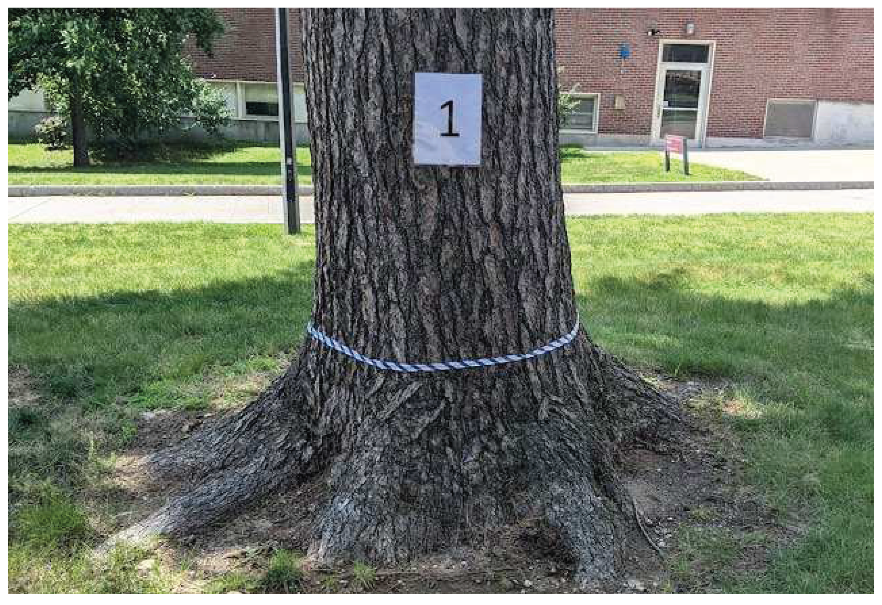
Figure 2. Output of Resistograph for tree 24, including the height at which the trunk was drilled, the diameter at that height, the average sound wood thickness from five drillings, and the ratio of sound wood thickness (T) to trunk radius (R) at each drilling (D) location.

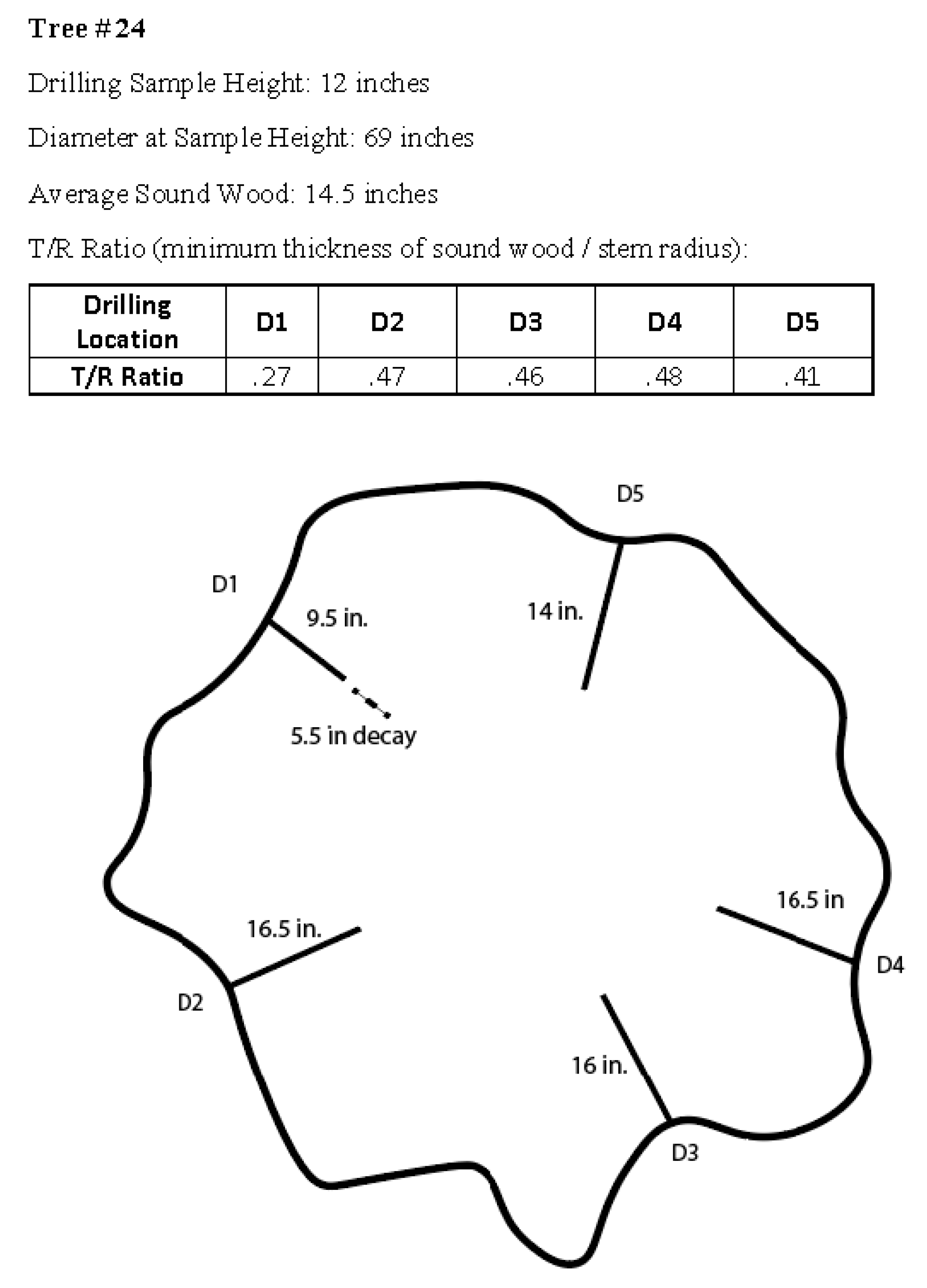
Figure 3. (a) Sonic and (b) electrical resistance tomograms of a tree; color coding along the top margin of the sonic tomogram indicates the areas of sound (in brown) and damaged (in violet and blue) wood expressed as proportions of the total cross-sectional area. Areas of green in the sonic tomogram represent intermediate velocities that are not utilized by the software to report the “damaged” cross sectional area. In the ER tomogram, areas of relatively lower electrical resistance (higher relative conductivity) appear as blue, while relatively higher resistance appear as red.

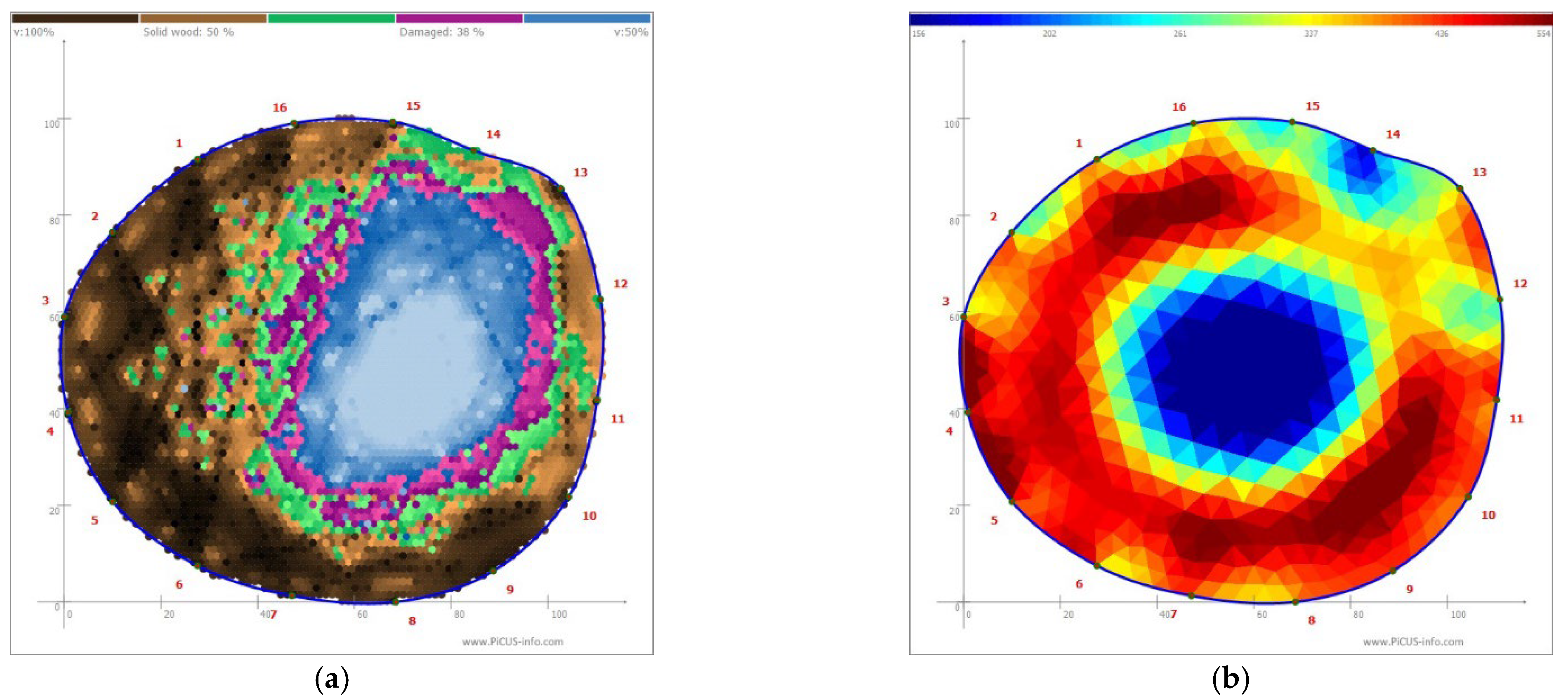
Figure 4. Proportional likelihood of failure ratings assigned following each assessment technique, which are listed, from left to right, in the order they were conducted for odd-numbered trees. For even-numbered trees, the tomogram assessment was conducted before the resistance drill assessment.

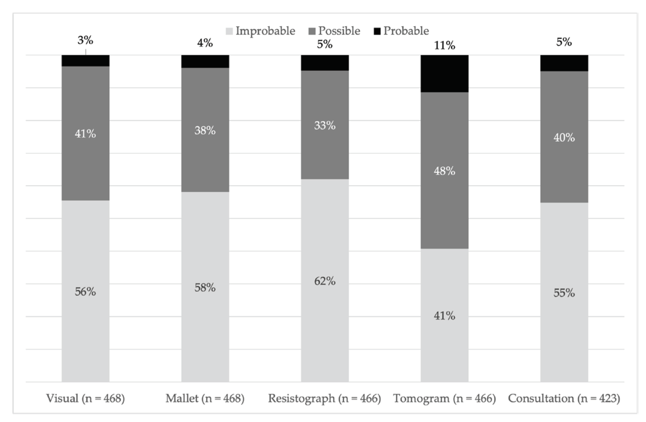
Figure 5. Proportional response of likelihood of failure ratings—improbable (light shading), possible (gray shading), probable (black shading)—vs. continuous covariates (left-hand panels: percent of the cross-section with decay, assessed by tomography; middle panels: average thickness of sound wood, assessed by Resistograph; right-hand panels: frequency that assessors employed resistance drilling in risk assessments) for each assessment technique. The vertical ordering of plots in columns labeled “Resistograph Assessment First” indicates the order in which assessments were conducted. The order was the same for plots in columns labeled “Tomography Assessment First” except that the tomography assessment preceded the Resistograph assessment. The presentation facilitates comparison between techniques for each covariate.

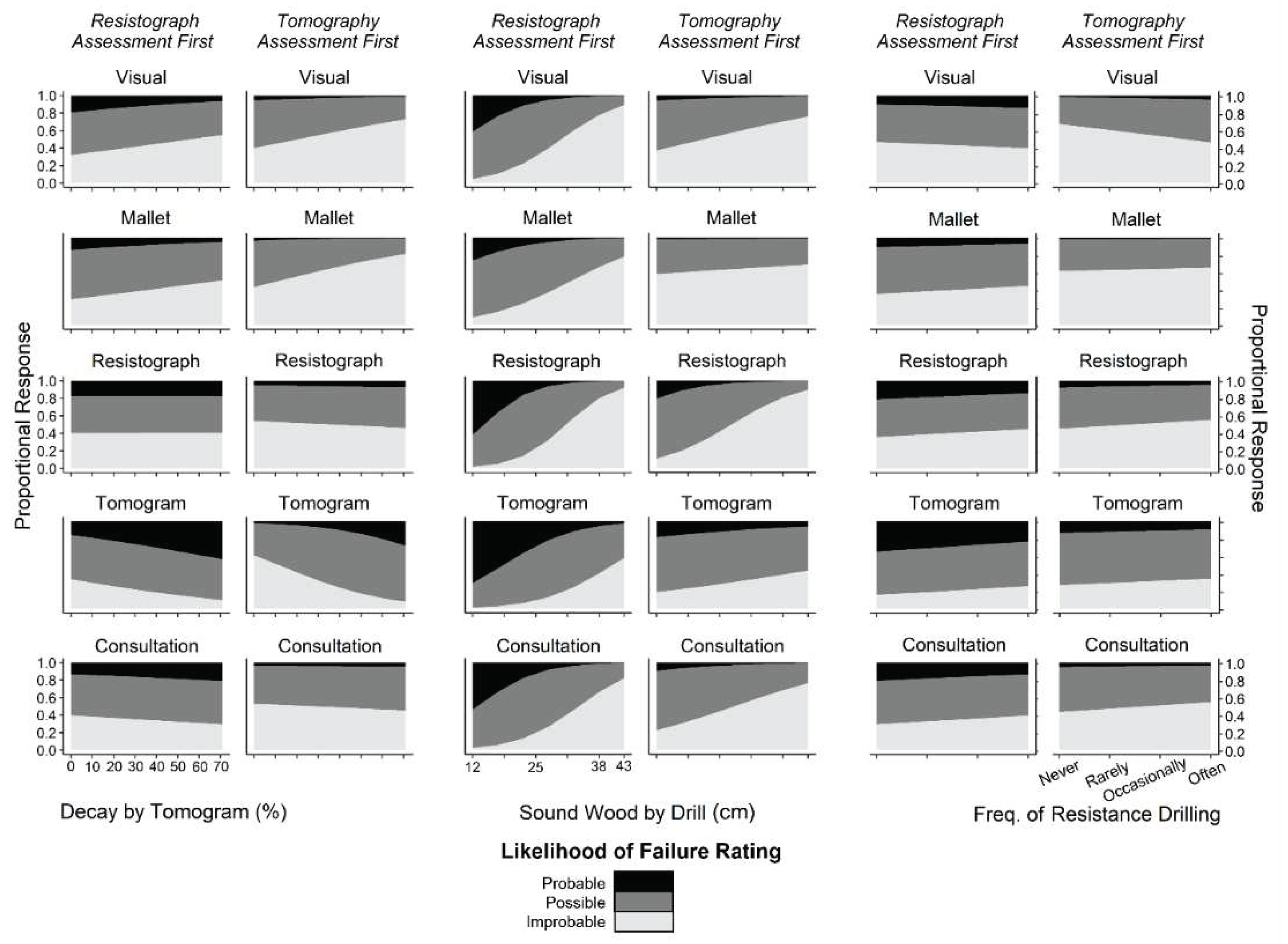
Figure 6. Proportional response of likelihood of failure ratings as related to how frequently assessors used tomography for risk assessments.

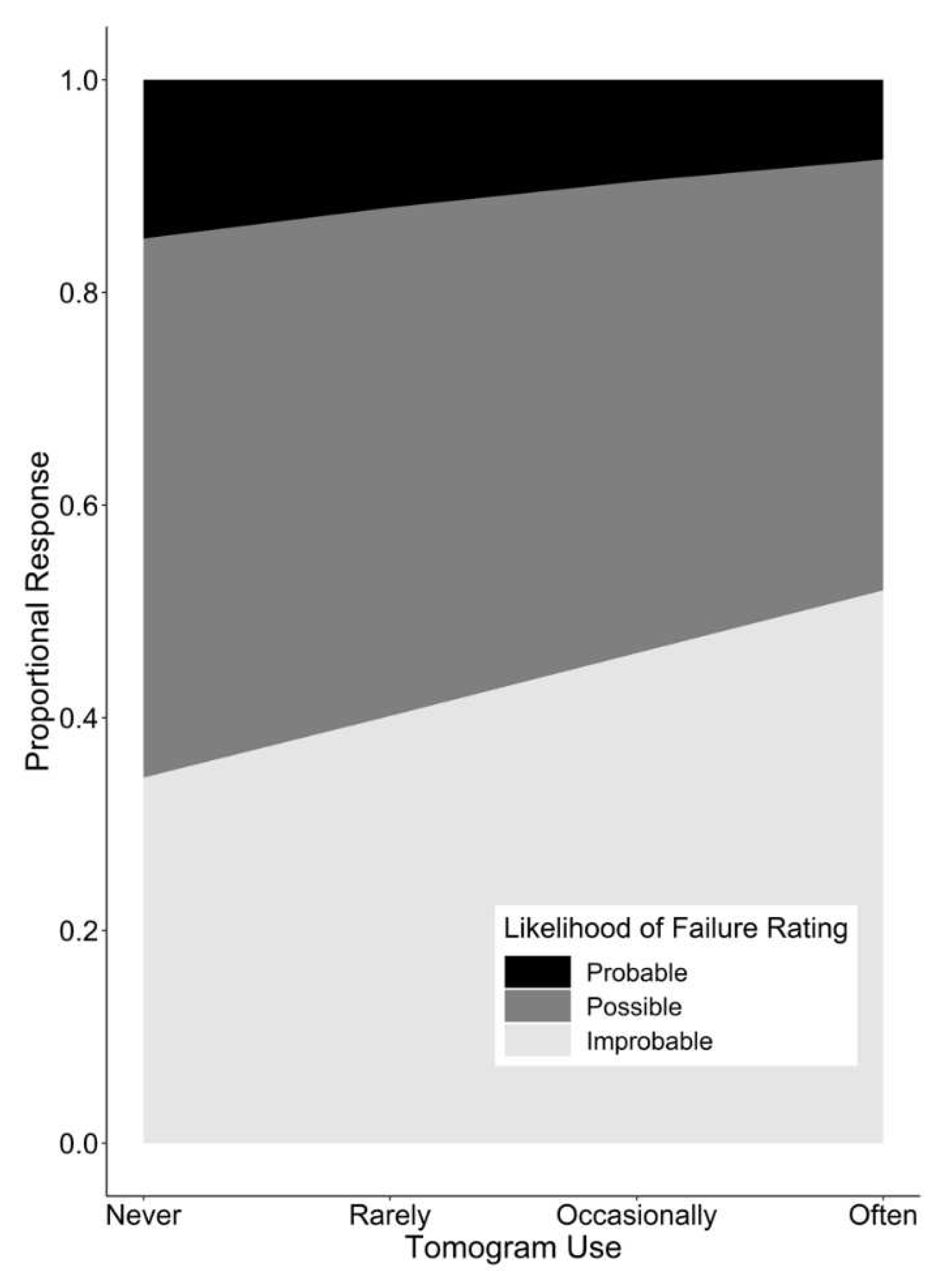
Figure 7. Factors that assessors reported as influencing their likelihood of failure ratings.

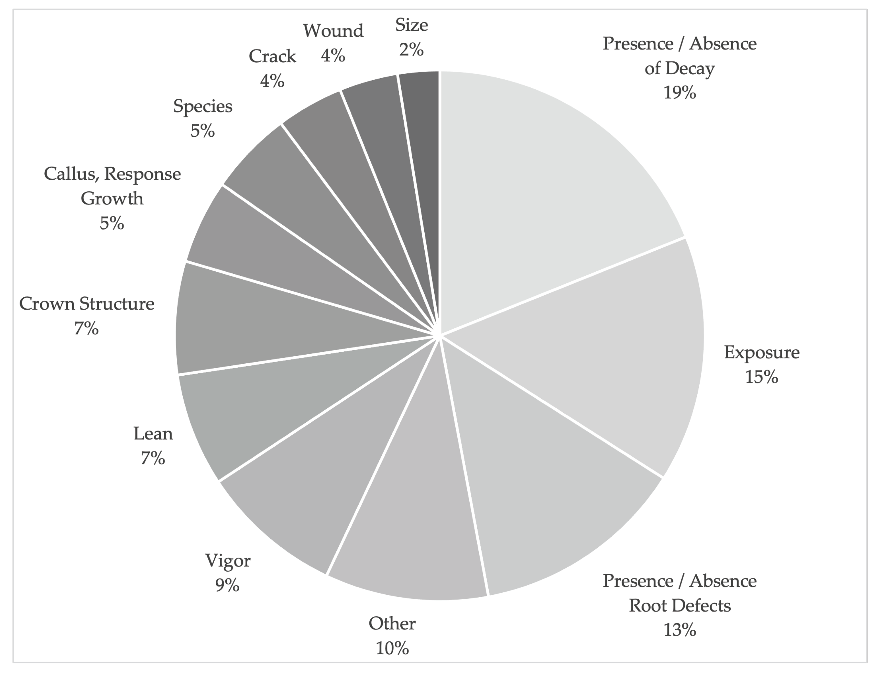
Figure 8. (a) Resistograph output of tree 22; (b) tomogram of tree 22; (c) Resistograph output of tree 27; (d) tomogram of tree 27.

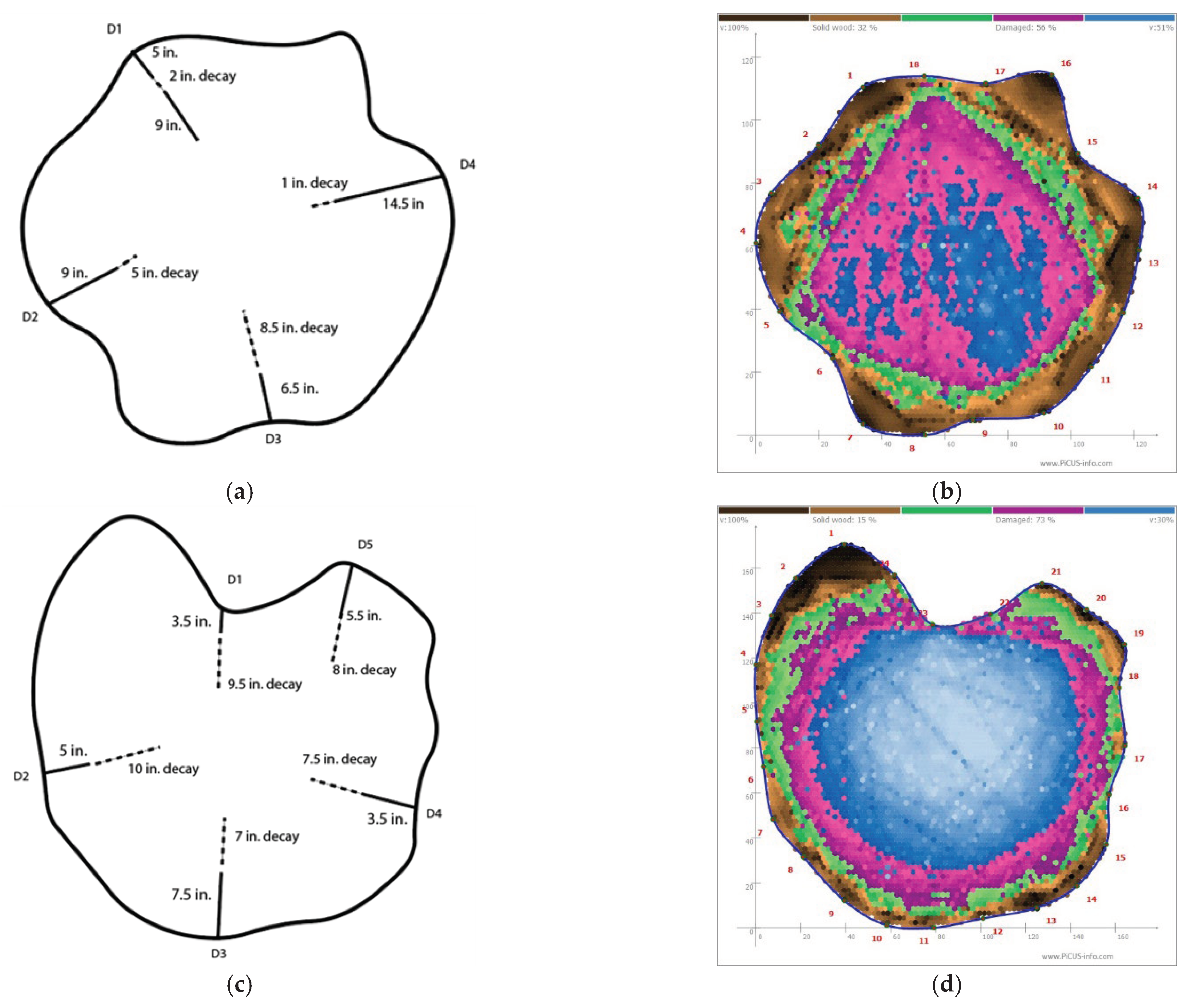
Figure 9. (a) Tree 3 in situ; (b) Resistograph output of tree 3; (c) tomogram of tree 3; (d) Tree 4 in situ; (b) Resistograph output of tree 4; (c) tomogram of tree 4.

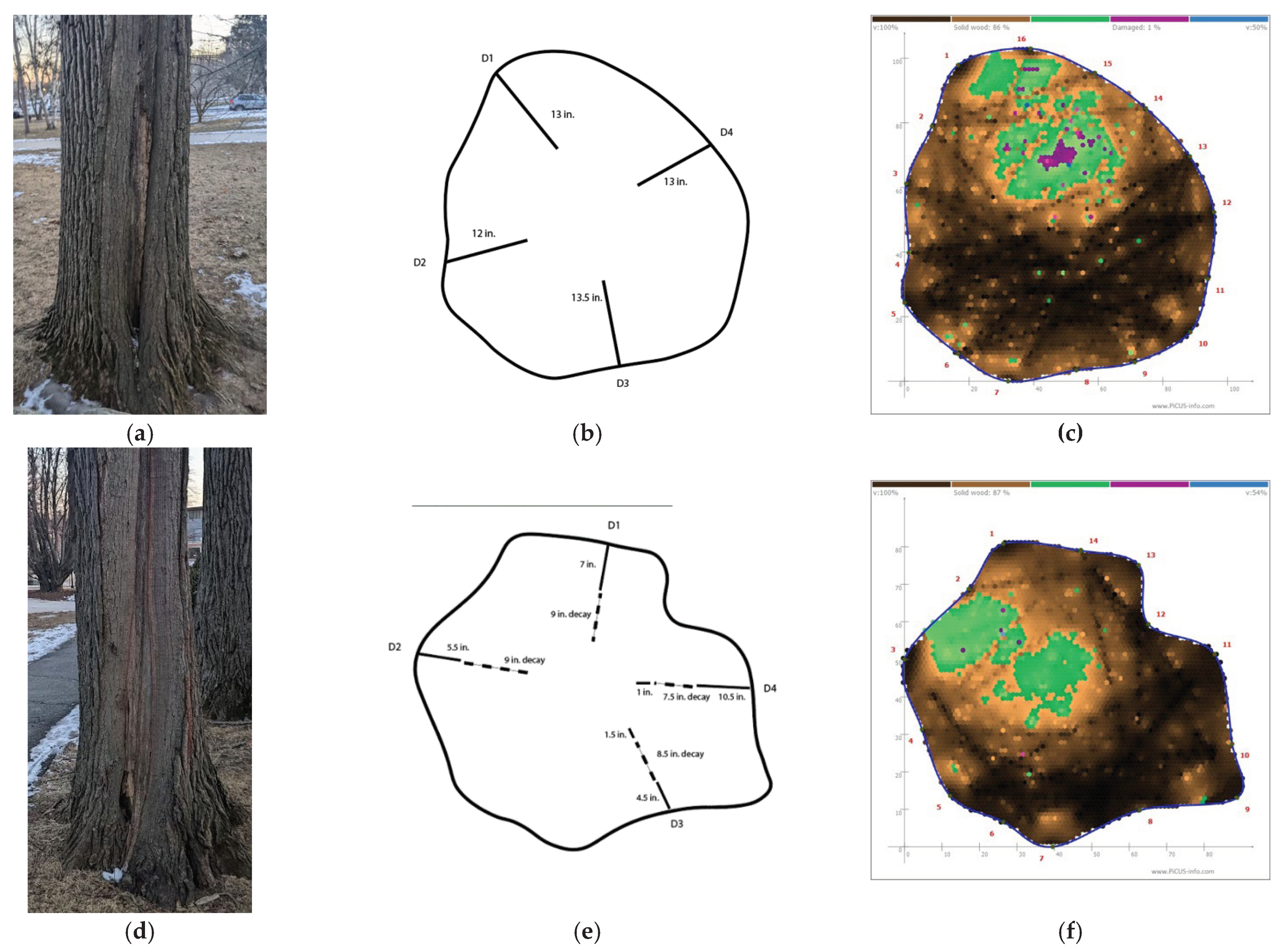
Table 1. Assessors’ (n = 18) frequency of use with techniques and tools used in the study.

Inquiry	Never	Rarely	Occasionally	Often
How frequently do you conduct basic visual risk assessments?	0	0	1	17
How frequently do you use a sounding mallet when conducting risk assessments?	0	0	2	16
How frequently do you use a resistance recording drill when conducting risk assessments?	2	4	4	8
How frequently do you use a sonic tomography system when conducting risk assessments?	1	5	5	7

Table 2. Morphological data for individuals of the two genera (Pinus and Quercus) in the study, including tree number, species, diameter 1.4 m above ground (DBH), tree height, crown width, height of tomography and Resistograph, mean thickness (t) of sound wood from Resistograph, minimum ratio of thickness of sound wood to stem radius (t/R), percentage of the stem cross-section with decay (% Decay) from the sonic tomogram, and percentage loss in section modulus (% Z_LOSS) from Burcham et al. (2019).

Tree	Species	DBH (cm)	Height (m)	Width (m)	Sample Height (cm)	t (cm)	t/R	% Decay	% Z_LOSS
1	P. strobus	89	24	14	50	31	0.5	26	16
2	Q. bicolor	84	20	28	30	25	0.5	0	0
3	Q. bicolor	71	17	15	30	31	0.6	1	1
4	Q. bicolor	69	17	13	30	18	0.2	13	0
5	Q. palustris	122	23	24	30	34	0.3	36	47
6	Q. rubra	76	17	9	30	29	0.2	18	21
7	Q. rubra	152	23	26	30	23	0.0	32	14
8	Q. alba	81	20	18	30	41	0.8	0	0
9	Q. alba	84	18	17	30	37	0.6	26	19
10	P. strobus	71	21	12	40	38	1.0	0	0
11	Q. palustris	84	23	19	30	40	0.6	49	32
12	Q. bicolor	91	20	14	30	36	0.1	40	77
13	Q. bicolor	91	23	14	30	30	0.3	63	54
14	P. strobus	97	24	16	100	45	0.9	0	0
15	P. strobus	66	20	11	50	38	1.0	0	4
16	Q. alba	61	19	8	30	34	0.7	0	0
17	Q. palustris	91	23	19	40	33	0.0	44	23
18	Q. palustris	97	25	23	40	20	0.0	53	65
19	Q. alba	107	21	20	30	40	0.6	71	73
20	Q. velutina	107	18	17	60	30	0.5	0	0
21	Q. velutina	145	26	25	50	22	0.0	65	92
22	Q. velutina	104	21	23	30	22	0.2	56	35
23	Q. bicolor	155	27	30	30	38	0.3	44	65
24	Q. rubra	124	21	27	30	37	0.3	66	88
25	Q. palustris	102	23	19	30	41	0.5	51	85
26	P. strobus	86	21	16	100	31	0.0	6	n/a ¹
27	Q. rubra	132	24	17	40	13	0.1	73	85
28	Q. velutina	74	20	10	30	33	0.2	12	20
29	Q. velutina	84	21	15	40	41	0.8	33	22
30	Q. velutina	94	24	17	40	30	0.0	37	81
Overall Mean		96	21	18	40	32	0.39	31	35
Odd-numbered trees ²		105	22	19	36	33	0.41	41	42
Even-numbered trees ³		88	21	17	43	31	0.37	20	28

¹ Not computed. ² The Resistograph assessment preceded the tomogram assessment. ³ The tomogram assessment preceded the Resistograph assessment.

Table 3. Analysis of variance table for the ordinal logistic regression model used to predict likelihood of stem failure rating from the main effect of assessment technique, covariates that quantified the random effects of trees and assessors, and their interactions; the table includes the χ² value of the likelihood ratio (LR) and the degrees of freedom (Df) and p-value of the effect or interaction.

Effect	LR χ²	Df	p-value
Technique	93.87	9	<0.0001
% Decay in cross-section	0.005	1	0.9419
Mean sound wood thickness	0.006	1	0.9404
Frequency of using a resistance drill	0.001	1	0.9780
Frequency of using tomography	4.279	1	0.0386
Genus	2.474	1	0.1157
Technique * % decay in cross-section	167.3	9	<0.0001
Technique * mean sound wood thickness	42.70	9	<0.0001
Technique * frequency of using a resistance drill	27.47	9	0.0012

Table 4. Analysis of variance table for beta dispersion tests for homogeneity of variance among (a) assessors’ self-reported frequency of sonic tomography use for tree risk assessment and (b) assessment techniques.

	Parameter	Df	Sum Sq	Mean Sq	F-value	p-value
(a)	Groups	17	0.07237	0.004257	1.1438	0.3173
	Residuals	162	0.60294	0.003722

(b)	Groups	3	0.00041	0.000135	0.0393	0.9896
	Residuals	176	0.60547	0.003440

Table 5. Distribution of the number of different likelihood of failure ratings (LoFRs) within each assessment technique.

	Assessment Technique ¹
Number of LoFRs	Visual	Mallet	Resistograph	Tomogram	Consultation
1	0	5	5	2	4
2	23	14	20	15	23
3	7	11	5	13	3

¹ From left to right, techniques are listed in chronological order for odd-numbered trees; for even-numbered trees, the tomogram assessment preceded the Resistograph assessment.

Table 6. For each assessment technique, the distribution of assessors’ responses to the question Did the technique change your likelihood of failure rating?

	Assessment Techniques After Visual Assessment ¹
Response	Mallet	Resistograph	Tomogram	Consultation
Yes	210	252	270	170
No	223	165	153	178

¹ From left to right, techniques are listed in chronological order for odd-numbered trees; for even-numbered trees, the tomogram assessment preceded the Resistograph assessment.

Table 7. For each tree and the four assessment techniques that followed the initial visual assessment (n = 120), the ratio (

R

) of the weighted mean change in likelihood of failure rating (LoFR) from the initial visual rating to the proportion of unchanged ratings for the tree and technique. Values in the upper quartile (underlined) indicate higher LoFRs than the initial visual assessment; values in the lower quartile (bolded) indicate lower LoFRs. Interquartile values in plain text indicate unchanged LoFRs.

Table 7. For each tree and the four assessment techniques that followed the initial visual assessment (n = 120), the ratio (

R

Tree	Consistent Basic Assessment ¹	Consistent Advanced Assessment ²	Consultation Confirmed ³	Mallet	Drill	Tomogram	Consultation
1	No	Yes	Neither	0.60	0.46	1.11	0.42
2	No	Yes	Advanced	-0.29	-0.38	-0.29	-0.31
3	Yes	Yes	Advanced	0.00	-0.70	-0.42	-0.78
4	Yes	No	Basic	-0.20	0.31	-0.30	-0.08
5	Yes	No	Basic	-0.13	-0.13	0.78	0.18
6	No	Yes	Advanced	-0.45	0.20	0.20	-0.11
7	No	No	Neither	-0.38	0.27	0.56	0.00
8	Yes	Yes	n/a	-0.14	-0.20	-0.14	-0.23
9	Yes	No	Neither	-0.17	-0.29	2.60	0.50
10	Yes	Yes	Advanced	-0.09	-0.80	-0.80	-0.36
11	Yes	No	Basic	0.33	0.08	0.89	0.44
12	No	No	Neither	-0.27	-0.27	0.83	-0.14
13	Yes	Yes	Advanced	0.25	0.78	6.00	0.60
14	No	No	Neither	1.50	-0.30	0.00	0.09
15	Yes	Yes	n/a	0.22	-0.25	-0.25	-0.20
16	Yes	Yes	n/a	-0.07	-0.07	-0.07	-0.07
17	Yes	Yes	Advanced	-0.15	0.50	2.20	0.75
18	Yes	Yes	Advanced	0.00	3.67	6.00	3.33
19	Yes	No	Basic	-0.18	-0.18	4.00	0.00
20	No	Yes	Advanced	-0.86	-6.00	-6.00	-3.67
21	Yes	Yes	Advanced	0.29	0.63	2.50	0.50
22	Yes	No	Basic	-0.08	0.44	13.00	0.20
23	Yes	No	Basic	0.30	-0.38	0.57	0.40
24	Yes	No	Basic	-0.17	0.08	2.20	0.18
25	Yes	No	Basic	0.33	0.09	1.00	0.25
26	No	Yes	Advanced	0.75	-0.67	-0.43	-0.80
27	No	No	Neither	-0.50	0.43	1.00	1.00
28	No	Yes	Advanced	-0.40	-3.67	-2.50	-2.25
29	Yes	No	Basic	0.27	-0.27	0.09	-0.20
30	Yes	Yes	n/a	-0.17	-0.11	0.40	0.25

¹ “Consistent” indicates that the LoFR assigned in the mallet assessment was the same as in the initial visual assessment. ² “Consistent” indicates that the advanced assessments (Resistograph and tomogram) produced the same change in LoFR from the initial visual assessment. ³ Confirmation of the advanced assessments occurred when the advanced and consultation assessments produced the same change in LoFR from the initial visual assessment; confirmation of the basic assessments occurred when the LoFRs assigned in the mallet and consultation assessments were unchanged from the initial visual assessment; “n/a” indicates that confirmation was not applicable because all LoFRs were unchanged from the initial visual assessment.

Disclaimer/Publisher’s Note: The statements, opinions and data contained in all publications are solely those of the individual author(s) and contributor(s) and not of MDPI and/or the editor(s). MDPI and/or the editor(s) disclaim responsibility for any injury to people or property resulting from any ideas, methods, instructions, or products referred to in the content.

© 2023 by the authors. Licensee MDPI, Basel, Switzerland. This article is an open access article distributed under the terms and conditions of the Creative Commons Attribution (CC BY) license (http://creativecommons.org/licenses/by/4.0/).

Copyright: This open access article is published under a Creative Commons CC BY 4.0 license, which permit the free download, distribution, and reuse, provided that the author and preprint are cited in any reuse.

MDPI Initiatives

Important Links

Choose an area of interest and we will send you notifications of new preprints at your preferred frequency.

Disclaimer