Submitted:
24 April 2023
Posted:
25 April 2023
You are already at the latest version
Abstract
Accelerators play a critical role in fostering innovative ecosystems and nurturing startups. The evaluation and selection of startups, particularly technology-based startups, for acceleration programs are essential in accelerator economy and management. Assessment of startups requires consideration of numerical and qualitative criteria such as sales, prior startup experience, demand validation, and product maturity. Startups must be ranked based on the varying importance of criteria, which can be identified as a fuzzy multi-criteria decision-making (MCDM) problem. MCDM methods have proven effective in managing complex problems. However, the use of MCDM techniques in startup selection and evaluation of criteria interrelationships from the accelerator perspective is yet to be researched. This study proposes a hybrid DEMATEL-ANP-based fuzzy PROMETHEE II model to rank startups and examine the interrelationships between factors. The final preference values are fuzzy numbers, making a fuzzy ranking method necessary for decision-making. An extension of ranking fuzzy numbers using a spread area-based relative maximizing and minimizing set is suggested to improve the flexibility of existing ranking MCDM methods. Algorithms and formulas are derived and a comparison demonstrates the merits of the proposed method. Finally, a numerical experiment is designed to address the viability of the hybrid DEMATEL-ANP-based fuzzy PROMETHEE II model.
Keywords:
DEMATEL
; ANP
; PROMETHEE II
; Ranking Fuzzy numbers
; Startups
1. Introduction
Entrepreneurship has been demonstrated to affect economic growth, directly and indirectly, and support more investments in knowledge creation and generation [1]. Notably, technology-based startups can transform the traditional economy into a digital economy through innovation [2]. The factors determining entrepreneurial success are entrepreneurs’ connections, leadership skills, financial competency, aptitude, knowledge, and support services [3]. Stam [3] defined the entrepreneurial ecosystem “as a set of interdependent actors and factors coordinated in such a way that they enable productive entrepreneurship.” Accelerators, whose mission is fostering innovation and nurturing startups, are the primary players in the entrepreneurial ecosystem. They develop startup projects, including financing, services, networking, mentoring, and training [4]. Not only do accelerators support networking services, mentorships, and education, but they also finance to augment entrepreneurial firms. Despite their critical role, research on how accelerators select entrepreneurial firms and their selection criteria is still limited [5].
The initial step of the entry-boost-exit process is to select a suitable startup. Accelerators invest in a selected startup, which means the accelerator’s profit depends on the startup’s exit; hence, accelerators must be selective when evaluating startup projects [5]. The three steps of the selection process are as follows: calling for startups’ submission, examining and assessing the projects, and, based on the opinions of the key decision-makers (DMs), rejecting inauspicious projects and investing in promising projects [6]. Lin et al. [7] used the hesitant fuzzy linguistic (HFL) multi-criteria decision-making (MCDM) method to evaluate startups from a technology business incubator perspective, taking into account DMs’ psychology. They developed a ratio of score value to deviation degree to compare HFL term sets and defined the HFL information envelopment efficiency, analysis, and preference model. Their numerical example showed the method’s applicability, and they concluded that it is more flexible and general. However, this method only applies to HFL information environments with unrevealed criteria weight values. The authors also stated that research on ranking startups is limited in the literature.
Selecting startups for acceleration programs involves incredibly complex qualitative criteria, such as competitive advantage and demand validation, and quantitative criteria, such as investment cost and the number of team members. Therefore, the ranking of startups is an MCDM problem. MCDM is a field of research that contributes to decision-support methodologies and tool development and execution [8]. Additionally, MCDM methods help resolve multiplex problems that involve objectives, multiple criteria, and alternatives rated by DMs. The DMs’ judgment through qualitative criteria is crucial to the decision-making process but can be subjective and vague. Hence, fuzzy numbers (FNs) can be used better to model human thought relative to their crisp counterparts.
However, an MCDM method only applies to classical mathematical theory, and different methods must be improved or combined to adapt to actual MCDM [9]. Moreover, the amalgamation of DEMATEL-ANP-based fuzzy PROMETHEE II has never been applied. This work aims to bridge this gap and investigates the technology startup selection procedure from the accelerators’ point of view using DEMATEL-ANP-based fuzzy PROMETHEE II. No study has scrutinized this hybrid method in evaluating startups; therefore, our study tested its feasibility and effectiveness. A ranking method based on spread areas is proposed with formulas to support the decision-making process, and a comparison demonstrates the method’s advantages. Subsequently, a numerical example clarifies the complete process of the hybrid method.
The remainder of the paper is organized as follows. Section 2 presents a literature review of the accelerator, selection criteria, and MCDM techniques. Section 3 presents the classical concept of fuzzy set theory and introduces the hybrid DEMATEL-ANP-based fuzzy PROMETHEE II method. Section 4 presents a comparative analysis to demonstrate the advantages of the ranking technique. Section 5 introduces a numerical example that highlights the viability and implementation of the hybrid approach in real-world problems. Finally, concluding thoughts and avenues for further research are presented in Section 6.
2. Literature review
2.1. Accelerators and the startup selection approach
In the last 15 years, accelerators have boomed due to their effects on startup development, entrepreneurial ecosystem formation, and innovation support [10]. The Y-Combinator, the first accelerator founded by Paul Graham in 2005, was a milestone for the growth of startup accelerators worldwide. By April 2023, according to Seed-DB, 8153 companies were accelerated with funding of US$88,874,580,633 [11]. Worldwide high-impact accelerators include Y-Combinator, with 1801 companies accelerated and US$52,211,811,615 of funding, Techstars with 1336 companies accelerated and US$12,690,624,018 of funding, and 500startups with 1686 companies accelerated and US$4,030,020,819 of funding. In the entrepreneurial ecosystem, many organizations support startups in their early stages with financial and nonfinancial investment, including incubators, accelerators, angel investors, venture capitalists, and governments. However, accelerators are the primary players with their mission of fostering innovative ecosystems and nurturing startups.
Accelerators provide mentoring and networking for selected startups in their intensive programs that develop startups’ ability to seek investors. “Accelerators are organizations that serve as gatekeepers and validators of promising business innovations through their embeddedness in their respective ecosystems and, thus, play an active and salient role in socioeconomic and technological advancement” ([10], p.2). Moreover, various accelerators require equity to counterbalance the support services. For example, the structured investment of one of the biggest accelerators, 500startups, is US$150,000 for 6% of their companies [12]. The primary return of profit-driven accelerators is from initial public offerings or acquisitions when a startup exits [13]. Therefore, accelerators must be selective when evaluating startup projects. The filtering process is crucial yet challenging for both accelerators and startups; however, research on the selection criteria and process is still lacking [5].
When investigating the Singapore-based Joyful Frog Digital Incubator (JFDI), Yin and Luo [5] adopted an RWW framework for innovation projects to apply to the accelerator program’s assessment. Using a scoreboard of 30 criteria based on the RWW framework, they identified eight vital criteria in the initial screening process. Among these factors, market attractiveness factors explain the existing markets and potential customers, including “demand validation,” “customer affordability,” and “market demographics,” and product feasibility factors include “concept maturity,” “sales and distribution,” and “product maturity.” In addition, product advantage factors, such as “value proposition” and “sustainable advantage,” and team competence factors, such as “technology expertise,” “prior startup experience,” and “feedback mechanism,” were crucial. Furthermore, “growth strategy” was considered an essential criterion.
Mariño-Garrido et al. [14] used statistical methods on a Spanish accelerator case study analysis to determine the essential criteria for selecting an entrepreneurial project. Out of the nine criteria investigated, six were significant: speed of acceleration, the extent of innovation, the extent of investment ability, creativity, negotiation, and the extent of team consistency.
2.2. MCDM methods
MCDM methods assist in resolving complex problems that entail multiple objectives, criteria, and alternatives evaluated by decision-makers (DMs). A review of MCDM methods can be found in various studies [15,16,17,18].
DEMATEL [19,20] is a constructive method for identifying cause–effect-linked components of a multiplex system. Using a visual systemic model, the technique evaluates interrelationships among criteria and uncovers the critical interrelationships. Moraga et al. [21] used DEMATEL to create a quantitative strategy map identifying causal relationships. Using an MCDM method, the authors developed the final strategy map with qualitative and quantitative approaches that improve and assist managers’ assessment process. Altuntas and Gok [22] applied DEMATEL to making correct quarantine decisions, aiming to reduce the burden of the COVID-19 pandemic on the hospitality industry. Wang et al. [23] suggested a new approach for group recommendation, named GroupRecD, which utilizes data mining and the DEMATEL technique to allocate user weights scientifically and rationally. Si et al. [24] conducted a systematic review of DEMATEL. They claimed that the DEMATEL has advantages, including effectively analyzing the direct and indirect effects among factors, visualizing the interdependent relationships between factors by network relation maps, and identifying critical criteria. However, the review also pointed out that DEMATEL cannot achieve the desired level of alternatives, as in Vise Kriterijumska Optimizacija I Kompromisno Resenje (VIKOR) method, or produce partial ranking sequences, as in the ELimination Et Choix Traduisant la REalite (ELECTRE) method. Hence, the DEMATEL was combined with different MCDM methods to obtain appropriate outcomes [24].
Saaty [25] introduced both the AHP and ANP methods. The AHP method [26] assumes criteria independence and analyzes decision-making problems in a hierarchical criteria structure. To overcome this limitation, Saaty [27,28] developed the ANP method, which considers dependencies and feedback among elements in a network structure to obtain criteria weights. A systematic review of both methods can be found in [29]. The ANP method has been applied to various fields of research. Galankashi et al. [30] amalgamated fuzzy logic and linguistic expression with ANP for investment portfolio selection. When sorting portfolios, multiple studies have focused on financial factors; however, the results indicated that other factors, such as risk, the market, and growth, are essential. The study demonstrated that ANP could present the internal relations between criteria, which is critical in decision-making. In 2023, Saputro et al. [31] utilized Multi-Dimensional Scaling (MDS) and ANP to examine the sustainability approach for developing rural tourism in Panjalu, Ciamis, Indonesia. Kadoić [32] noted that the ANP method effectively analyzes interconnections and consistency within a decision system. Criteria weights should be identified before alternative weights to prevent fraud and irregularities [32].
The Preference Ranking Organization Method for Enrichment Evaluations (PROMETHEE), developed by Brans [33], is one of the most common MCDM methods. PROMETHEE was extended to decision-making in many studies, such as PROMETHEE I for partial ranking and PROMETHEE II for complete ranking [34]. The method has undergone many modifications and improvements to assist humans in decision-making [35]. Among them, PROMETHEE II is the most frequently used because it allows a DM to establish a full ranking [36]. The PROMETHEE methods have also been applied to FNs. Jiang et al. [37] proposed a PROMETHEE II method based on covering-based variable precision fuzzy rough sets with fuzzy logical operators. Hua and Jing [38] extended the classical PROMETHEE method by incorporating the generalized Shapley value in interval-valued Pythagorean fuzzy sets to achieve a more rigorous ranking outcome. To verify the effectiveness of this approach, a case study is conducted to evaluate sustainable suppliers.
Numerous studies have applied hybrid models combining the PROMETHEE method and other MCDM techniques. For example, Khorasaninejad et al. [39] used a hybrid model to determine the best prime mover in a thermal power plant. The model combined fuzzy ANP-DEMATEL to assess criteria importance and relationships and PROMETHEE to rank alternatives. Govindan et al. [40] used an integrated Fuzzy Delphi, a DEMATEL-based ANP (DANP), and a PROMETHEE method to choose the best supplier based on corporate social responsibility practices and to identify the key factors. Torbacki [41] applied the crisp DANP and PROMETHEE II methods to assess cybersecurity in the sustainable Industry 4.0 sphere. The literature review indicated that combining DEMATEL, ANP, and PROMETHEE methods is effective and reliable in assisting decision-making in various fields. However, DEMATEL-ANP-based fuzzy PROMETHEE II amalgamations have never been applied. In this research, DEMATEL is adopted during the first stage to investigate the cause–effect relationships between criteria and to filter out the nonsignificant criteria. Then, ANP is used to determine the criterion weights because it permits criterion dependency. Finally, the fuzzy-based PROMETHEE II method determines the final ranking.
2.3. Ranking fuzzy numbers
Lofi Zadeh [42] introduced fuzzy sets to efficiently model human thought. Fuzzy sets have widely affected many areas of scientific research, including mathematics [43], engineering [44], business, and management [45]. A literature review of the historical evolutions of fuzzy sets, their application, and their frequencies was conducted by Kahraman et al. [46].
Ranking FNs became a critical problem in linguistic decision-making. Jain [47] proposed the first FN ranking method based on maximizing sets. Since then, various methods have been presented, such as the Pos index and its dual Nec index [48], maximizing set and minimizing set [49], area compensation [50], an area method using a radius of gyration [51], deviation degree [52], defuzzified values, heights and spreads [53] and mean of relative values [54].
Wang et al. [52] proposed a ranking method based on left and right deviation degrees derived from maximal and minimal reference sets. Additionally, Wang and Luo [55] introduced an area ranking method using positive and negative ideal points, which they claimed more effectively discriminated FNs than Chen’s maximizing and minimizing sets [49]. Asady [56] pointed out that the methods of Wang et al. [52] could not correctly rank fuzzy images. Therefore, he proposed a revised method using parametric forms. Nejad and Mashinchi [57] developed a technique based on the left and right areas to improve the deviation degree method. Yu et al. [58] proposed an extension using an epsilon-deviation degree. Nevertheless, Chutia [59] observed that the approach of Yu et al. still presented limitations in discriminating FNs. Chutia suggested a modified method constituting the ill-defined magnitude value and the angle of the fuzzy set. However, this method cannot be used when FNs have non-linear left and right membership functions [59]. Ghasemi et al. [60] discovered a disadvantage in both the deviation degree method [52] and area ranking based on positive and negative ideal points [55]. The author accordingly introduced an improved approach that considers DMs’ risk attitudes. Moreover, numerical examples that demonstrated the efficiency of ranking the proposed method’s FNs were provided.
Chu and Nguyen [61] suggested a method to improve Chen’s [49] maximizing and minimizing sets to rank FNs. In their study, comparative examples were provided. An experiment demonstrated that the relative maximizing and minimizing set (RMMS) could consistently and logically rank the final fuzzy values of alternatives. This study proposed a fuzzy ranking approach inspired by area ranking and using four spread areas. Based on the RMMS model, the areas were measured and integrated with a confidence level μ to assist the FN ranking procedure. The DMs provided confidence levels, which indicated their confidence toward alternatives.
3. Model Establishment
3.1. Fuzzy Set Theory
3.1.1. Fuzzy Sets
where x is an element in the space of points U,
A is a fuzzy set in U, is the membership function of A at x [71]. The larger , the stronger the grade of membership for x in A.
3.1.2. Fuzzy Numbers
A real FN A is described as any fuzzy subset of the real line R with a membership function that possesses the following properties [58]. is a continuous mapping from R to [0,1],. is strictly increasing on the left membership function and is strictly decreasing on the right membership function . and
, where a, b, c, and d are real numbers.
We may let , or a=b, or b=c, or c=d, or d=. Unless elsewhere defined, A is assumed to be convex, normalized, and bounded, i.e., , . A can be indicated as , . Let represent and represent the left and the right membership function of A, respectively, and
In this research, TFNs will be used. The FN A is a TFN if its membership function is given as follows [72].
where a, b and c are real numbers.
3.1.3. α-Cuts
The α-cuts of FN A can be determined as, where is a non-empty bounded closed interval is contained in R and can be denoted by, where are lower bounds and are upper bounds [62].
3.1.4. Arithmetic Operations on Fuzzy Numbers
Given FNs A and B,, and . By the interval arithmetic, some primary operations of A and B can be described as follows [62].
3.1.5. Linguistic Values
A linguistic variable is a variable whose values are represented in linguistic terms. It is advantageous for dealing with complicated matters or is ambiguous to be rationally described in traditional quantitative information [49,63]. DMs are assumed to have agreed to weight alternatives over criteria using linguistic values such as Extremely Poor (EP), Very Poor (VP), Poor (P), Moderate (M), High (H), Very High (VH), and Extremely High (EH) which can also be represented by TFNs such as EP=(0,0.1,0.25), VP=(0.1,0.2,0.35), P=(0.25,0.35,0.5), M=(0.35,0.5,0.65), H=(0.5,0.65,0.75), VH=(0.65,0.8,0.9), and EH=(0.75,0.9,1).
3.1.6. Relative Maximizing and Minimizing Sets
Chu and Nguyen [61] suggested a technique to improve Chen’s [49] maximizing and minimizing set to rank FNs. In their study, numerical comparisons and example were conducted to demonstrate that the RMMS can consistently and logically rank fuzzy values of alternatives. The RMMS [61] technique is introduced as follows.
Assume there are n FNs,. , FNs and are added to the right and left sides of the above n FNs , respectively. Assume , , and . Let and , where , , , . The new supremum element is defined as and the new infimum element is defined as , where .
The relative maximizing set and the relative minimizing set are determined as:
Herein, k is set to 1. The value of k can be varied to suit the application. The total relative utility of each Ai is denoted as in Eq. (8).
where the first right relative utility , the first left relative utility , the second left relative utilityand the second right relative utility.
3.1.7. Spread area-based RMMS
In 2011, Nejad and Mashinchi [57] pointed out the shortcomings of Wang et al.’s [52] deviation degree method that when the values of the left area, the right area, the transfer coefficient or is zero, the ranking result is inaccurate. Hence, to prevent these problems from occurring, expanding and is needed when ranking. Chu and Nguyen [61] also found out that when adding a new FN, and must be modified by adding equal values to consider both sides of membership functions. Consequently, four utilities need to be accounted for to reduce the inconsistency of Chen’s [49] maximizing and minimizing set. However, if a set of FNs with , then a new FN is added, there is no extended value applicable in this situation. Therefore, this work suggests to integrate confidence level in ranking FNs to solve the mentioned problems.
Yeh and Kuo [64] in their research on evaluating passenger service quality of Asia-Pacific international airports, suggested incorporating a DM’s confidence level α and a preference index λ to obtain an overall service performance index. In the evaluation procedure, DMs give the value α, based on the concept of an α-cut, with respect to the criteria’s weights and alternative performance ratings.
This work proposes to use confidence level in a new perspective, which is confidence level, symbolized as μ, will be integrated into measuring areas spreading based on the RMMS model to assist the ranking FNs procedure, as shown in Figure 1. First, h experts in the group of DMs, are asked to specify their confidence , representing their confidence for alternatives to obtain . The greater the μ, the more assured is the decision-maker on the alternative.
Since DMs’ confidence in an alternative will influence their confidence level in other alternatives, the confidence level μ, calculated by the average of all DMs’ evaluation, should be engaged simultaneously to the immensity of the RMMS concept. Accordingly, value μ is integrated by shifting the RMMS’s infimum element to the left, provided that the new infimum element is obtained as . Similarly, the average value of μ will be integrated by shifting the RMMS’s infimum element to the right, provided that the new supremum element is obtained as .
The coordinates of the intersect of the with the relative maximizing set and the relative minimizing set can be seen in Figure 1 and are determined as the following equations.
The first left spread area is defined as follows.
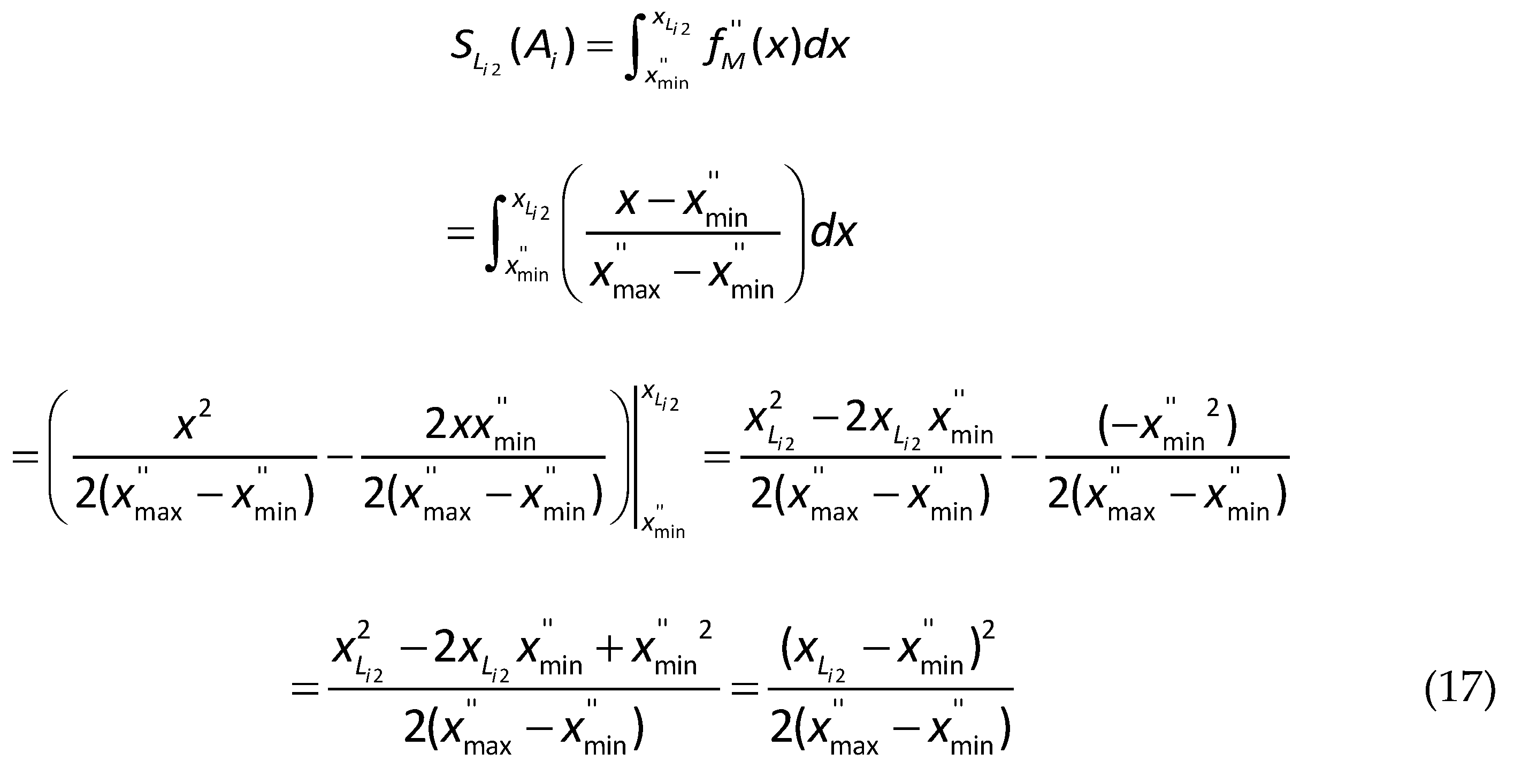
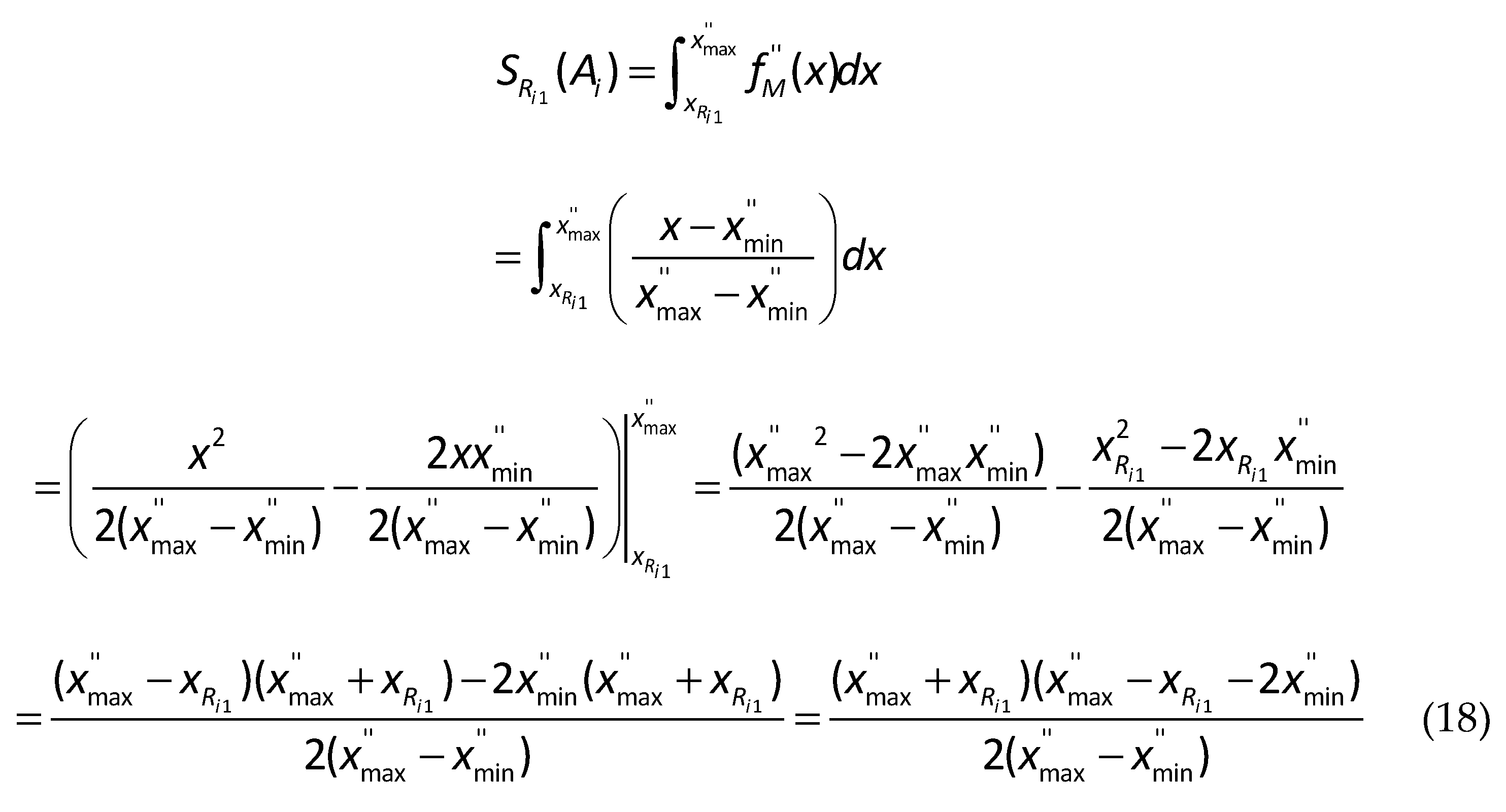
Clearly, if the first left spread area is larger, fuzzy number is larger. The second left spread area is defined as Eq. (14); and if is larger, fuzzy number is also larger. The first right spread area is defined as Eq. (15); but if is lager, fuzzy number is smaller. Finally, the second right spread area is defined as Eq. (16); and if is larger, fuzzy number is also smaller. Therefore, the above four areas must be considered when ranking FNs. The detailed derivation for Eqs. (14)-(16) is placed in Appendix I.
Finally, the ranking value of each is determined as Eq. (17) to classify FNs. An FN is more prominent if its value is larger.
3.1.8. The hybrid DEMATEL-ANP based fuzzy PROMETHEE II model
DEMATEL
The DEMATEL method is first used to demonstrate the interrelationships between criteria and produce the influential network relationship map. The constructing equations of the classical DEMATEL model can be summarized as follows [65].
Assume that h experts in a decision groupare asked to indicate the direct effect of factor (criterion) Ci has on factor (criterion) Cj in a system with m factors (criteria)using an integer scale of No Effect (0), Low Effect (1), Medium Low Effect (2), Medium Effect (3), Medium High Effect (4), High Effect (5) and Extremely Strong Effect (6). Next, the individual direct-influence matrix provided by the eth expert can be constructed, where all main diagonal components are equal to zero and represent the respondent’s evaluation of DM on the degree to which criterion Ci affects Cj.
Step 1. Generating the group direct-influence matrix. By aggregating h DMs’ judgments, the group direct-influence matrix can be constructed by)
Step 2. Acquiring the normalized direct-influence matrix. At this step, the normalized direct influence matrix by the eth expert is .
The following equations calculate the average matrix X
Step 3. Computing the total-influence matrix T. The total-influence matrix is computed the summation of the direct impacts and all of the indirect impacts by Eq. (21)
(21)
when in identity matrix, named as I.
Step 4. Setting up a threshold value and producing the causal diagram.
The sum of columns and the sum of rows are symbolized as R and D, respectively, within the total-relation matrix by the following formulas
The horizontal axis vector (D + R) called “Prominence” demonstrates the power of influence degree that is given and received by the criteria. The vertical axis vector (D - R) named “Relation” shows the system’s criteria effect. If (D – R) is positive, the criterion Cj influences other criteria and can be grouped into a causal group; if (D + R) is negative, the criterion Cj is being influenced by the other criteria and can be grouped into an effect group. A causal diagram can be produced by mapping the (D + R, D - R) dataset, yielding valuable assessment perception. A threshold value can be defined to screen out the negligible factors [66,67]. In this work, factors that have a value higher than the average value of the “Prominence” (D + R) and/or (D – R) is positive are selected to use in the next step.
ANP
Next, the present work applied the ANP method to produce the weights of the criteria. The generalized ANP process from previous studies is summarized as follows [27,68,69]. In this work, a set of importance scales [13] is adopted to weight each criterion using linguistic values, including 1 –Identically Important (II), 3 – Moderately Important (MI), 5 – Highly Important (HI), 7 – Very Highly Importance (VHI), 9 – Extremely Important (EI), and 2, 4, 6, 8 are the median values. Reciprocal values are used for inverse comparison.
Step 1. Obtaining Pairwise Comparison Matrix (PCM). Assume that h experts in a decision group are responsible for evaluating criteriathat are screened through the previous step. The PCM is generated by comparing the ith row with the jth column. The weights of components are formed as shown in matrix A. The diagonal components having identical importance are illustrated by 1.
As there are several DMs, the pairwise comparison values from different DMs may vary. Experts can decide together or each assessment can be integrated into a PCM by the geometric mean GM as in Eq. (24).
Step 2. Computing eigenvectors and unweighted supermatrix. In this step, eigenvector Ei is obtained through Eq. (25), which is computed by each row’s average.
Then, the eigenvectors of each matrix are consolidated to form the unweighted matrix.
Step 3. Examining the consistency. In order to guarantee consistency among the judgments of the DMs, it is necessary to test the consistency by three metrics, including Consistency Measure (CM), Consistency Index (CI), and Consistency Ratio (CR).
The general form for CM values is obtained through Eq. (26).
where aj is the corresponding row of the comparison matrix, E is Eigenvector and Ej represents the corresponding component in E.
Then, λmax is obtained by the average of the CM vector. The CI is calculated as shown in Eq. (27).
Next, a random index, as listed in Table 1 [13], is computed following the order of the PCM. Consequently, the consistency ratio CR is obtained by Eq. (28).
The value of CR ≤ 0.1 is in the satisfactory range; otherwise, the pairwise comparison is required to be revised.
Step 4. Obtain the weighted supermatrix. A weighted supermatrix is obtained to evaluate the relation between criteria. Then, the unweighted matrix is converted into a weighted supermatrix to make the sum of each column be 1, called column stochastic.
Step 5. Determining stable weights by obtaining limit supermatrix. The values produced from the previous step are elevated to the power of 2k until the values are firmly established, where k is an arbitrarily large number. The final priorities can be determined by using the normalization function on each block of the limit matrix. The most significant value represents the most critical criterion among other criteria. The stable weights w constructed from this step are utilized in the following steps.
Fuzzy PROMETHEE-based ranking method
The same group of h experts will assess n alternativesunder m criteriathat are screened through the previous steps. Let be the rating assigned to an alternative under the criterion by a decision-maker. Criteria chosen from the earlier steps are first categorized into the cost-benefit framework as qualitative benefit criteria, quantitative benefit criteria, cost qualitative criteria, and cost quantitative criteria The fuzzy PROMETHEE II process is summarized as follows [70,71].
Step 1. Constructing the fuzzy decision matrix. Aggregated rating is:
where , , .
Step 2. Computing the normalized matrix. The normalization is completed using the Chu and Nguyen [61] approach. The ranges of normalized TFNs belong to [0,1]. Suppose is the value of an alternative versus a benefit (B) criterion or a cost (C) criterion. The normalized value lij can be as
where .
Step 3. Calculating the evaluative differences. Pairwise comparison is made by calculating the evaluative differences of ith alternative with respect to other alternatives. The intensity of the fuzzy preference of an alternative Ai over Ai’ is obtained by Eqs. (32)-(33), based on Eq. (3)
where Pj is the fuzzy preference function for the jth criterion and Cj(Ai) is the evaluation of alternative Aicorresponding to criterion Cj.
Step 4. Determining the preference function. To avoid the complexity and be more in a practicable form, the simplified fuzzy preference function is applied in this study as in Eqs. (34) - (35).
Step 5. Reckoning the aggregated fuzzy preference function. Calculate the aggregated fuzzy preference function considering the criteria weights computed from the ANP method.
The higheris, the stronger preference for the ith alternative will be.
Step 6. Determining the fuzzy leaving flowand the fuzzy entering flow The fuzzy leaving flow of Ai is determined as
The fuzzy entering flow of Ai is determined as
Step 7. Calculating the fuzzy net outranking flow for each alternative
Step 8. Defuzzifying the fuzzy net outranking flow value and obtaining the ranking of alternatives. In this step, the spread area-based RMMS model is proposed to apply to assist defuzzification and obtain the final ranking using Eqs. (12)-(20). An FN is more prominent if its value is more significant.
4. Numerical Comparison and Consistency Test
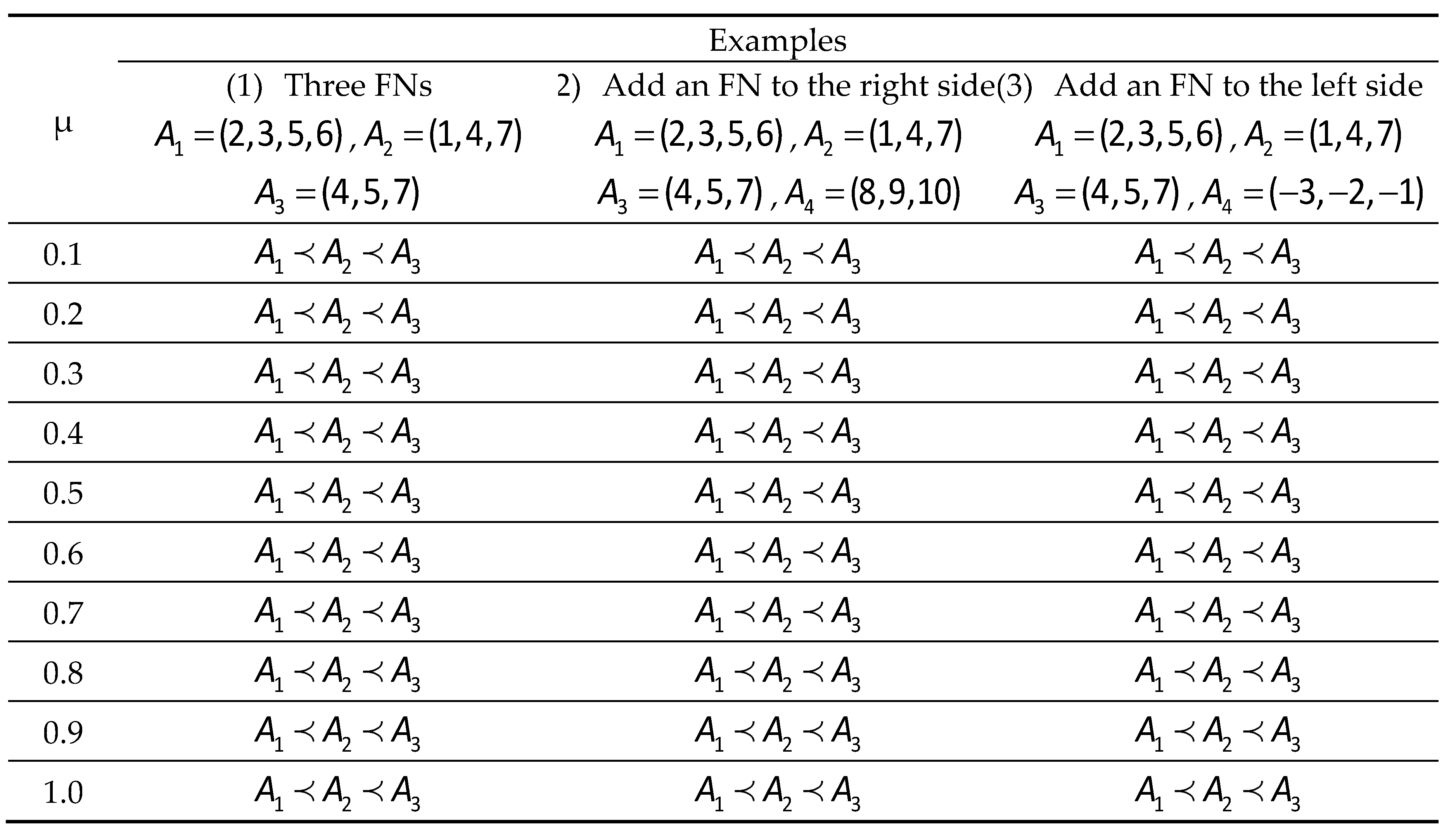
In this section, various examples of comparisons are established to investigate the effectiveness of the proposed method. The first example illustrates the ranking orders of the method compared with the methods of Wang et al. [52] and Nejad and Mashinchi [57]. We used FNs in Examples 2, 3, and 4 from Nejad and Mashinchi [57], and then different situations were generated through the addition of new FNs for testing the consistency of the ranking results, as shown in Table 2. In Situation (1), methods from both Nejad and Mashinchi and Wang et al. produce , but the proposed method can discriminate between three FNs with the order . Furthermore, the ranking order is , and either is added (see Situation [1.1]) or is added (see Situation [1.2]). In Situation (2), the proposed method yields the same ranking, , as that of the method of Nejad and Mashinchi when either or is added. However, the method of Wang et al. highlights the inconsistency and produces in Situation (2.2). In Situation (3), the proposed method yields the same ranking as that of Nejad and Mashinchi when or is added, but the method of Wang et al. compensates for the inconsistency and produces in Situation (3.2). The first comparison demonstrates the usefulness of the proposed method in discriminating FNs.
Second, three sets of FNs are created to further examine the proposed method’s stability and credibility, as shown in Table 3. In all previous situations, the method of Wang et al. is ineffective in distinguishing FNs. For example, in Situation (1.1), the method of Nejad and Mashinchi yields an FN ranking, , but yields in cases (1) and (1.2), indicating inconsistency, but the proposed method yields in all Situations (1), (1.1), and (1.2). Similarly, in Situations (2) and (2.2), the ranking order obtained using the method of Nejad and Mashinchi is ; however, when is added, the order changes to , as in Situation (2.1); whereas the suggested method persistently ranks in the following order: . In Situations (3) and (3.2), both the proposed method and the method of Nejad and Mashinchi yield a ranking order of ; however, in (3.1), whenis added, the method of Nejad and Mashinchi yields ; however, the proposed method yields a persistent rank order of. Hence, the second comparison has demonstrated the effectiveness of the proposed method in discriminating FNs compared to Wang et al.’s technique and the consistency compared with the method of Nejad and Mashinchi.
Additionally, a consistency test is designed to examine the reliability of the proposed method, as shown in Table 5. In Example 1, the result is for all assumed various µ values. In Example 2, when is added, the classifying order remains the same as for all . Finally, in Example 3, whenis added, the proposed method consistently yields an order of for all tested values of µ. The results of the numerical comparison demonstrate the credibility and effectiveness of the suggested ranking method based on spread area–based RMMS.

Table 5.
A consistency test with various values of µ in different examples.
5. Numerical Example
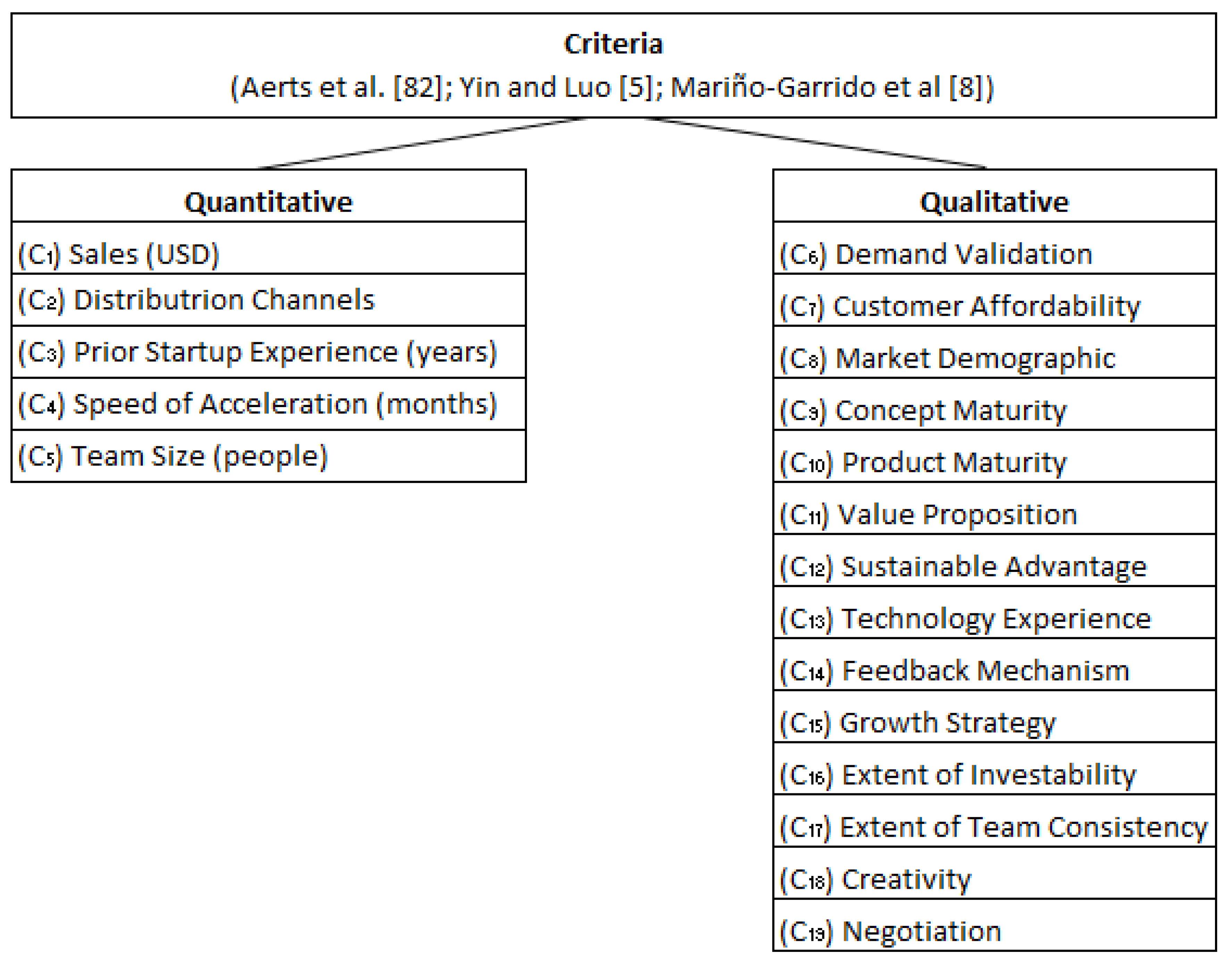
Suppose 4 DMs of an accelerator must establish criteria and analyze the criteria’s effect on a technology-based acceleration program. To achieve this goal, the methods DEMATEL and ANP are performed. Assume are the qualitative criteria and quantitative criteria under consideration, as shown in Figure 2 (see Appendix II for details). Assuming that DMs have reached a consensus, the effects of criteria on each other are indicated using a scale of No Effect (1), Low Effect (2), Medium Low Effect (3), Medium Effect (4), Medium High Effect (5), High Effect (6), and Extremely Strong Effect (7). After each DM rates the alternatives, the aggregating direct-relation matrix is determined using Eq. (18) and is shown in Table 6 (see Appendix III for details).
Subsequently, values of the normalized direct-relation matrix are obtained using Eqs. (19) and (20) and are shown in Table 7 (see Appendix IV for details). Finally, the total relation matrix is attained using Eq. (21), as shown in Table 8 (see Appendix V for details). Next, the prominence (D+R) and relation (D-R) values are calculated using Eqs. (22) and (23). Thereafter, the threshold value is set, which determines the filtered factors. The causal relationship and notable factors are displayed in Table 9 and Figure 3. According to Table 9, “(C6) demand validation” has the greatest (D+R) value and is the most critical factor, followed by “(C7) customer affordability” and “(C8) market demographic.” All these factors are necessary to be evaluated in the initial steps when building a product or service. Additionally, the (D-R) values of “(C3) prior startup experience,” “(C1) sales,” and “(C2) product development cost” demonstrate that these criteria have net influences on other factors. Other medium value factors that are selected when proceeding to the next steps are “(C9) concept maturity,” “(C10) product maturity,” “(C11) value proposition,” “(C13) technology experience,” “(C15) growth strategy,” “(C18) creativity,” and “(C19) negotiation.”
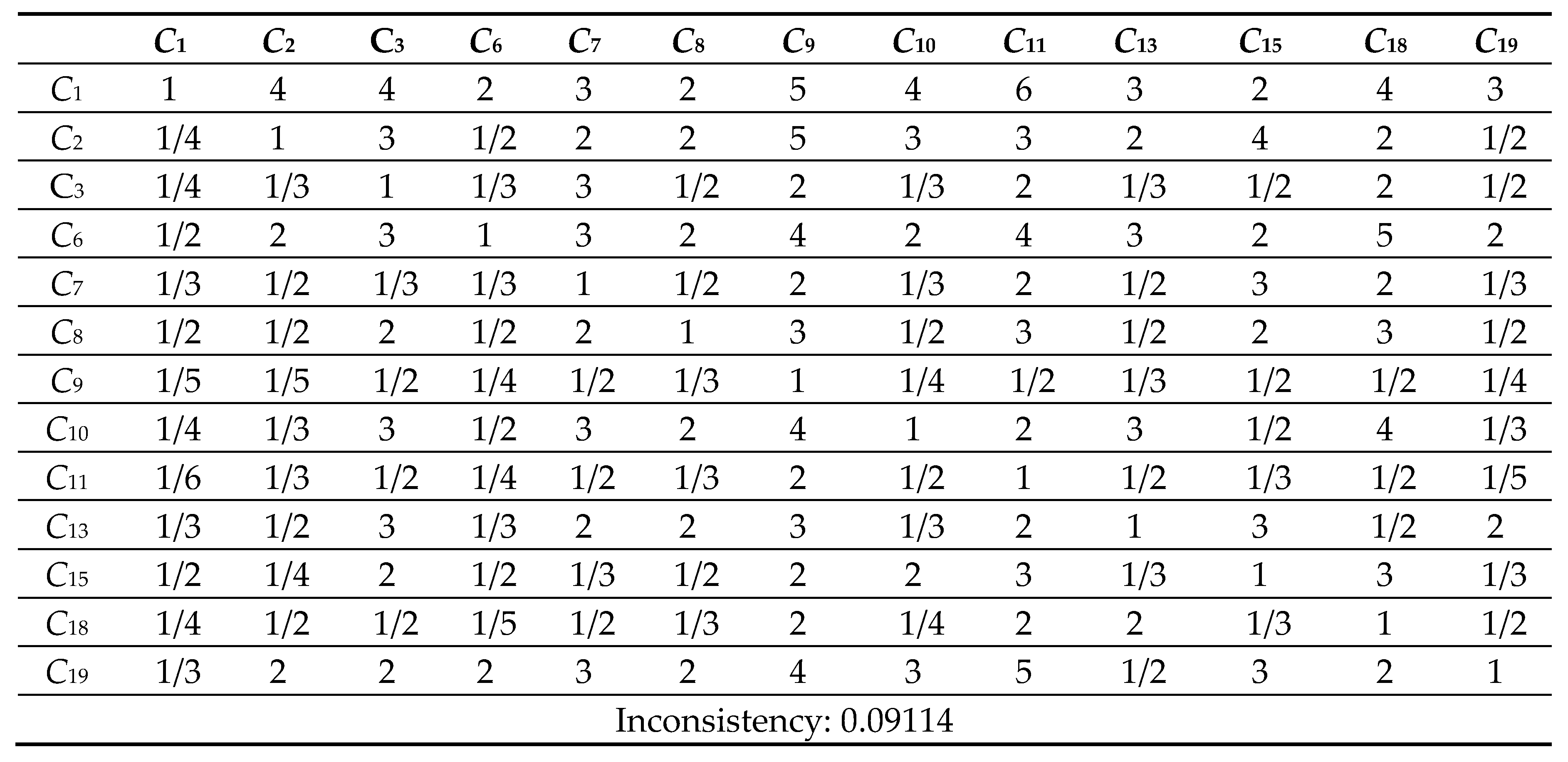
Next, the pairwise comparison must be carefully evaluated by DMs according to the criteria. In this study, the statistical software Super Decisions was used for the analysis. Super Decisions is a decision support program that implements AHP and ANP to calculate the weights of the dimensions and tests the expert’s competency. After obtaining the integrated PCM, the values are entered into the software to compute CR values. First, the integrated matrix is computed with respect to each criterion, including the consistency ratio CR ≤ 0.1, as shown in Eqs. (24) to (28) (see Tables 10.1–10.13 in Appendix VI for details). Then, the unweighted supermatrix and weighted matrix are created, as shown in Table 11 and Table 12. Finally, the limited matrix with the stable weights and the final weight order can be determined, as shown in Table 13 and Table 14. According to Table 14, “(C8) market demographics” has the highest value with 0.1253, followed by “(C6) demand validation” with 0.1196 and “(C3) prior startup experience” with 0.0940. The lowest weight value is “(C11) value proposition” with 0.0215.
Table 11.
The unweighted supermatrix.
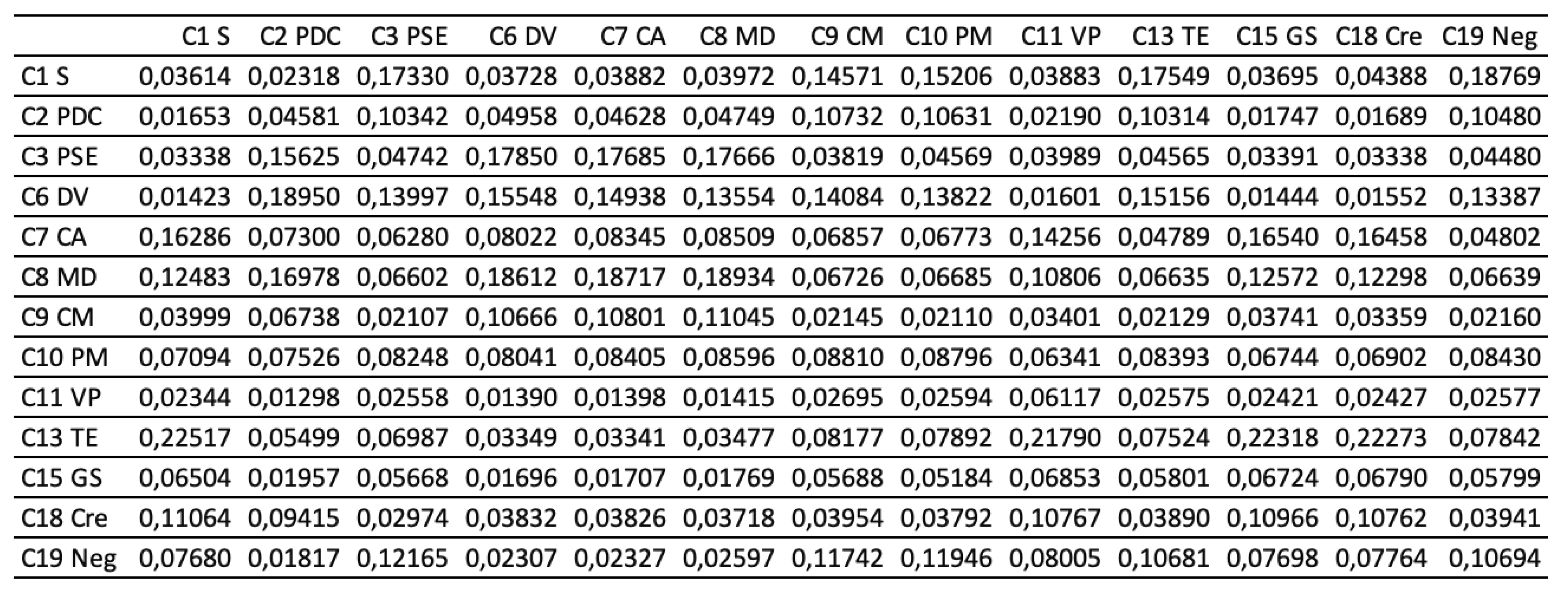
Table 12.
The weighted supermatrix.
Table 13.
The limited supermatrix.
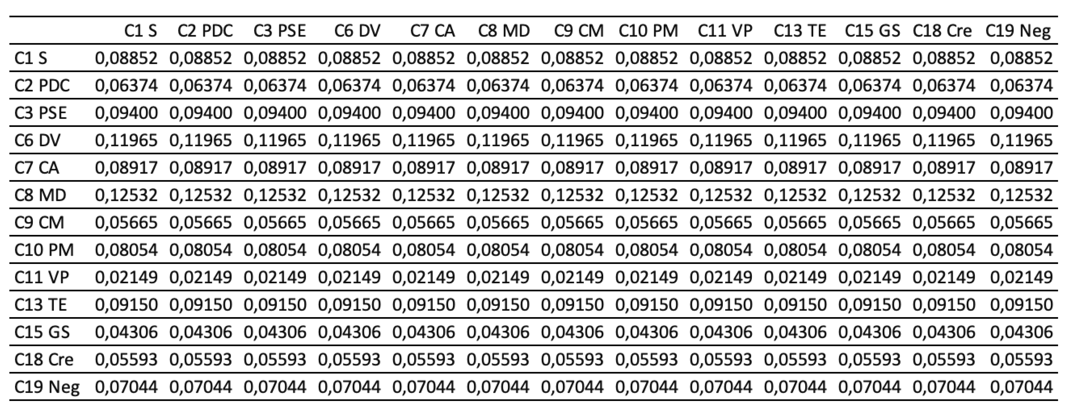
Table 14.
Final weight order.
| Criteria | Symbol | Values | Ranking |
| (C8) Market Demographic | C8 MD | 0.1253 | 1 |
| (C6) Demand Validation | C6 DV | 0.1196 | 2 |
| (C3) Prior Startup Experience | C3 PSE | 0.0940 | 3 |
| (C13) Technology Experience | C13 TE | 0.0915 | 4 |
| (C7) Customer affordability | C7 CA | 0.0892 | 5 |
| (C1) Sales | C1 S | 0.0885 | 6 |
| (C10) Product Maturity | C10 PM | 0.0805 | 7 |
| (C19) Negotiation | C19 Neg | 0.0704 | 8 |
| (C2) Product Development Cost | C2 PDC | 0.0637 | 9 |
| (C9) Concept Maturity | C9 CM | 0.0567 | 10 |
| (C18) Creativity | C18 Cre | 0.0559 | 11 |
| (C15) Growth Strategy | C15 GS | 0.0431 | 12 |
| (C11) Value Proposition | C11 VP | 0.0215 | 13 |
Finally, the fuzzy PROMETHEE II-based spread area
ranking method is applied. Suppose the same DM group assesses four
technology-based startup projects  under
13 criteria that are screened during the previous steps. The ratings of the
alternatives over qualitative criteria and quantitative criteria are shown in
Table 15 and Table 17
(see
Appendix V
II and
Appendix V
III, respectively,
for details). Subsequently, the mean ratings are calculated using Eq. (29), as
shown in
Table 16
, and the alternatives’ normalized gradings versus quantitative criteria
are produced using Eqs. (30) and (31), as shown in
Table 18
. The confidence
level ratings on alternatives are also collected to produce µ value, as
shown in
Table 19
.
under
13 criteria that are screened during the previous steps. The ratings of the
alternatives over qualitative criteria and quantitative criteria are shown in
Table 15 and Table 17
(see
Appendix V
II and
Appendix V
III, respectively,
for details). Subsequently, the mean ratings are calculated using Eq. (29), as
shown in
Table 16
, and the alternatives’ normalized gradings versus quantitative criteria
are produced using Eqs. (30) and (31), as shown in
Table 18
. The confidence
level ratings on alternatives are also collected to produce µ value, as
shown in
Table 19
. The aggregated fuzzy preference is attained using Eqs. (32) to (36), as shown in Table 20. Subsequently, the fuzzy leaving flow , the fuzzy entering flow , and the fuzzy net outranking flow for each alternative are computed using Eqs. (41) to (43), as presented in Table 21. Using the proposed spread area-based RMMS model, the fuzzy net outranking flow of each alternative is defuzzified using Eqs. (9) to (17) and yields values of A1 (−0.0519), A2 (0.0905), A3 (0.0594) and A4 (−0.0980). The final ranking of four startup projects indicates that startup project A2 has the highest comprehensive potential, followed by startup project A3.
The utilization of the DEMATEL-ANP-based fuzzy PROMETHEE II provides a comprehensive procedure for ranking alternatives. The DEMATEL investigated the cause–effect relationships between criteria and filtered out the nonsignificant criteria. Subsequently, ANP helped to determine the criteria weights because it permits criterion dependency. Finally, the final ranking was generated by the fuzzy-based PROMETHEE II method, which includes a proposed ranking model to enhance consistency and discrimination ability. The numerical results demonstrated the feasibility of the hybrid model for various decision-making management applications.
6. Conclusions
Language has naturally evolved to reflect human judgment and fuzzy ranking is required to turn assessments into decision-making. An extension on ranking FNs using spread area-based RMMS was proposed to improve the applicability and differentiation of the methods of Wang et al. [51], Nejad and Mashinchi [56], and Chu and Nguyen [60]. The algorithm and equations were derived by implementing a ranking method. Comparative examples demonstrated the strengths of the proposed method in discriminating fuzzy numbers and consistency ranking. Finally, the suggested ranking method was integrated into a hybrid DEMATEL-ANP-based fuzzy PROMETHEE II model to inspect the interrelationships among factors, obtain critical criteria weights, and organize startups for a comprehensive decision-making procedure. The numerical example has illustrated the feasibility of the hybrid fuzzy MCDM method. In future studies, the proposed fuzzy ranking method can be amalgamated into different MCDM methods to further investigate its validity and apply the method to various practices, such as project selections, evaluating business investments, evaluating accelerators, etc.
Author Contributions
Conceptualization, H.T.N. and T.-C.C.; methodology, H.T.N and T.-C.C.; validation, H.T.N. and T.-C.C.; formal analysis, H.T.N.; investigation, H.T.N. and T.-C.C.; resources, T.-C.C.; data curation, H.T.N.; writing—original draft preparation, H.T.N.; writing— review and editing, H.T.N. and T.-C.C.; visualization, H.T.N.; supervision, T.-C.C.; project administration, T.-C.C. All authors have read and agreed to the published version of the manuscript.
Funding
This work was supported in part by the National Science and Technology Council, Taiwan, under Grant MOST 111-2410-H-218-004.
Institutional Review Board Statement
Not applicable.
Informed Consent Statement
Not applicable.
Data Availability Statement
Not applicable.
Acknowledgments
Conflicts of Interest
The authors declare no conflict of interest.
Appendix I
The derivation of Eq. (17) for the second left spread areais presented as follows.
The derivation of Eq. (18) for the first right spread area is presented as follows.
The derivation of Eq. (19) for the second right spread area is presented as follows.

Appendix II
Figure 2.
Structure of criteria.
Appendix III
Table 6.
The aggregating direct-relation matrix of decision makers.
| C1 | C2 | C3 | C4 | C5 | C6 | C7 | C8 | C9 | C10 | C11 | C12 | C13 | C14 | C15 | C16 | C17 | C18 | C19 | |
| C1 | 0 | 2 | 1.5 | 4 | 5 | 1 | 1 | 1 | 1.5 | 1 | 2.75 | 4 | 4 | 3 | 2 | 5 | 3 | 3 | 3 |
| C2 | 5.5 | 0 | 1.25 | 5 | 4 | 1.25 | 1 | 1.75 | 1.25 | 2 | 1 | 4 | 2 | 3 | 1 | 4 | 2 | 2 | 2 |
| C3 | 6 | 6 | 0 | 6 | 6 | 4 | 5 | 4 | 3 | 3 | 4 | 6 | 5 | 6 | 6 | 5 | 6 | 5 | 5 |
| C4 | 4 | 3 | 1 | 0 | 4 | 1 | 1.75 | 1 | 2 | 1 | 2 | 3 | 1 | 5 | 2 | 3 | 3 | 4 | 2 |
| C5 | 3 | 4 | 1 | 4 | 0 | 1.75 | 2 | 2 | 1 | 2 | 1 | 4 | 4 | 6 | 1 | 2 | 3 | 5 | 4 |
| C6 | 6 | 6 | 4 | 5.75 | 6 | 0 | 4.25 | 4.5 | 6 | 6 | 6 | 6 | 4 | 5.75 | 6 | 6 | 5.75 | 5.25 | 3.75 |
| C7 | 6 | 6 | 3 | 6 | 6 | 3.75 | 0 | 3.25 | 6 | 5.75 | 5.75 | 6 | 6 | 6 | 5.25 | 5.5 | 6 | 4.75 | 3.75 |
| C8 | 5.75 | 6 | 4 | 5.75 | 5.25 | 3.5 | 4.75 | 0 | 5.5 | 5.25 | 6 | 5.5 | 4 | 6 | 5.75 | 6 | 5.75 | 5 | 3.75 |
| C9 | 6 | 6 | 5 | 6 | 6 | 1.5 | 1 | 2.5 | 0 | 6 | 5 | 6 | 3.25 | 6 | 6 | 6 | 5 | 4 | 4 |
| C10 | 6 | 6 | 5 | 6 | 5.75 | 1 | 1 | 2.25 | 2 | 0 | 5 | 6 | 3 | 6 | 5 | 5 | 6 | 3 | 4 |
| C11 | 5.25 | 6 | 4 | 6 | 6 | 2 | 2 | 1.75 | 2.75 | 3 | 0 | 6 | 5 | 5 | 3 | 6 | 4 | 3 | 3 |
| C12 | 4 | 4 | 1 | 4.75 | 4 | 1 | 1 | 1 | 1 | 2 | 2 | 0 | 2 | 3 | 2 | 4 | 4 | 2 | 3 |
| C13 | 4 | 6 | 3 | 6 | 4 | 4 | 2 | 4 | 4.75 | 5 | 3 | 6 | 0 | 6 | 6 | 5 | 5 | 6 | 6 |
| C14 | 5 | 5 | 2 | 3 | 2 | 2.25 | 2 | 1.5 | 1.75 | 1.75 | 3 | 5 | 1 | 0 | 1 | 2 | 2 | 1 | 3 |
| C15 | 6 | 6 | 2 | 6 | 6 | 1 | 2.75 | 2 | 1.75 | 3 | 5 | 6 | 2 | 6 | 0 | 6 | 6 | 2 | 3 |
| C16 | 3 | 4 | 3 | 5 | 6 | 2 | 1.75 | 1 | 2 | 3 | 2 | 4 | 3 | 6 | 1 | 0 | 3 | 2 | 2 |
| C17 | 5 | 6 | 2 | 5 | 5 | 1.75 | 2 | 2 | 3 | 2 | 4 | 4 | 3 | 6 | 2 | 5 | 0 | 3 | 2 |
| C18 | 4.75 | 5.75 | 3 | 4 | 3 | 2.75 | 3 | 3 | 4 | 5 | 5 | 6 | 2 | 6 | 6 | 6 | 5 | 0 | 5 |
| C19 | 5 | 6 | 3 | 6 | 4 | 4 | 4 | 4 | 4 | 4 | 5 | 5 | 2 | 5 | 5 | 6 | 6 | 3 | 0 |
Table 7.
The normalized direct-relation matrix.
| C1 | C2 | C3 | C4 | C5 | C6 | C7 | C8 | C9 | C10 | C11 | C12 | C13 | C14 | C15 | C16 | C17 | C18 | C19 | |
| C1 | 0 | 0.0206 | 0.0155 | 0.0412 | 0.0515 | 0.0103 | 0.0103 | 0.0103 | 0.0155 | 0.0103 | 0.0284 | 0.0412 | 0.0412 | 0.0309 | 0.0206 | 0.0515 | 0.0309 | 0.0309 | 0.0309 |
| C2 | 0.0567 | 0 | 0.0129 | 0.0515 | 0.0412 | 0.0129 | 0.0103 | 0.0180 | 0.0129 | 0.0206 | 0.0103 | 0.0412 | 0.0206 | 0.0309 | 0.0103 | 0.0412 | 0.0206 | 0.0206 | 0.0206 |
| C3 | 0.0619 | 0.0619 | 0 | 0.0619 | 0.0619 | 0.0412 | 0.0515 | 0.0412 | 0.0309 | 0.0309 | 0.0412 | 0.0619 | 0.0515 | 0.0619 | 0.0619 | 0.0515 | 0.0619 | 0.0515 | 0.0515 |
| C4 | 0.0412 | 0.0309 | 0.0103 | 0 | 0.0412 | 0.0103 | 0.0180 | 0.0103 | 0.0206 | 0.0103 | 0.0206 | 0.0309 | 0.0103 | 0.0515 | 0.0206 | 0.0309 | 0.0309 | 0.0412 | 0.0206 |
| C5 | 0.0309 | 0.0412 | 0.0103 | 0.0412 | 0 | 0.0180 | 0.0206 | 0.0206 | 0.0103 | 0.0206 | 0.0103 | 0.0412 | 0.0412 | 0.0619 | 0.0103 | 0.0206 | 0.0309 | 0.0515 | 0.0412 |
| C6 | 0.0619 | 0.0619 | 0.0412 | 0.0593 | 0.0619 | 0 | 0.0438 | 0.0464 | 0.0619 | 0.0619 | 0.0619 | 0.0619 | 0.0412 | 0.0593 | 0.0619 | 0.0619 | 0.0593 | 0.0541 | 0.0387 |
| C7 | 0.0619 | 0.0619 | 0.0309 | 0.0619 | 0.0619 | 0.0387 | 0 | 0.0335 | 0.0619 | 0.0593 | 0.0593 | 0.0619 | 0.0619 | 0.0619 | 0.0541 | 0.0567 | 0.0619 | 0.0490 | 0.0387 |
| C8 | 0.0593 | 0.0619 | 0.0412 | 0.0593 | 0.0541 | 0.0361 | 0.0490 | 0 | 0.0567 | 0.0541 | 0.0619 | 0.0567 | 0.0412 | 0.0619 | 0.0593 | 0.0619 | 0.0593 | 0.0515 | 0.0387 |
| C9 | 0.0619 | 0.0619 | 0.0515 | 0.0619 | 0.0619 | 0.0155 | 0.0103 | 0.0258 | 0 | 0.0619 | 0.0515 | 0.0619 | 0.0335 | 0.0619 | 0.0619 | 0.0619 | 0.0515 | 0.0412 | 0.0412 |
| C10 | 0.0619 | 0.0619 | 0.0515 | 0.0619 | 0.0593 | 0.0103 | 0.0103 | 0.0232 | 0.0206 | 0 | 0.0515 | 0.0619 | 0.0309 | 0.0619 | 0.0515 | 0.0515 | 0.0619 | 0.0309 | 0.0412 |
| C11 | 0.0541 | 0.0619 | 0.0412 | 0.0619 | 0.0619 | 0.0206 | 0.0206 | 0.0180 | 0.0284 | 0.0309 | 0 | 0.0619 | 0.0515 | 0.0515 | 0.0309 | 0.0619 | 0.0412 | 0.0309 | 0.0309 |
| C12 | 0.0412 | 0.0412 | 0.0103 | 0.0490 | 0.0412 | 0.0103 | 0.0103 | 0.0103 | 0.0103 | 0.0206 | 0.0206 | 0 | 0.0206 | 0.0309 | 0.0206 | 0.0412 | 0.0412 | 0.0206 | 0.0309 |
| C13 | 0.0412 | 0.0619 | 0.0309 | 0.0619 | 0.0412 | 0.0412 | 0.0206 | 0.0412 | 0.0490 | 0.0515 | 0.0309 | 0.0619 | 0 | 0.0619 | 0.0619 | 0.0515 | 0.0515 | 0.0619 | 0.0619 |
| C14 | 0.0515 | 0.0515 | 0.0206 | 0.0309 | 0.0206 | 0.0232 | 0.0206 | 0.0155 | 0.0180 | 0.0180 | 0.0309 | 0.0515 | 0.0103 | 0 | 0.0103 | 0.0206 | 0.0206 | 0.0103 | 0.0309 |
| C15 | 0.0619 | 0.0619 | 0.0206 | 0.0619 | 0.0619 | 0.0103 | 0.0284 | 0.0206 | 0.0180 | 0.0309 | 0.0515 | 0.0619 | 0.0206 | 0.0619 | 0 | 0.0619 | 0.0619 | 0.0206 | 0.0309 |
| C16 | 0.0309 | 0.0412 | 0.0309 | 0.0515 | 0.0619 | 0.0206 | 0.0180 | 0.0103 | 0.0206 | 0.0309 | 0.0206 | 0.0412 | 0.0309 | 0.0619 | 0.0103 | 0 | 0.0309 | 0.0206 | 0.0206 |
| C17 | 0.0515 | 0.0619 | 0.0206 | 0.0515 | 0.0515 | 0.0180 | 0.0206 | 0.0206 | 0.0309 | 0.0206 | 0.0412 | 0.0412 | 0.0309 | 0.0619 | 0.0206 | 0.0515 | 0 | 0.0309 | 0.0206 |
| C18 | 0.0490 | 0.0593 | 0.0309 | 0.0412 | 0.0309 | 0.0284 | 0.0309 | 0.0309 | 0.0412 | 0.0515 | 0.0515 | 0.0619 | 0.0206 | 0.0619 | 0.0619 | 0.0619 | 0.0515 | 0 | 0.0515 |
| C19 | 0.0515 | 0.0619 | 0.0309 | 0.0619 | 0.0412 | 0.0412 | 0.0412 | 0.0412 | 0.0412 | 0.0412 | 0.0515 | 0.0515 | 0.0206 | 0.0515 | 0.0515 | 0.0619 | 0.0619 | 0.0309 | 0 |
Appendix V
Table 8.
The total relation matrix.
| C1 | C2 | C3 | C4 | C5 | C6 | C7 | C8 | C9 | C10 | C11 | C12 | C13 | C14 | C15 | C16 | C17 | C18 | C19 | |
| C1 | 0.0681 | 0.0911 | 0.0507 | 0.1117 | 0.1165 | 0.0406 | 0.0418 | 0.0417 | 0.0532 | 0.0539 | 0.0754 | 0.1097 | 0.0820 | 0.1040 | 0.0655 | 0.1147 | 0.0891 | 0.0780 | 0.0781 |
| C2 | 0.1152 | 0.0620 | 0.0442 | 0.1134 | 0.1000 | 0.0391 | 0.0381 | 0.0450 | 0.0462 | 0.0580 | 0.0532 | 0.1018 | 0.0581 | 0.0954 | 0.0504 | 0.0979 | 0.0727 | 0.0631 | 0.0629 |
| C3 | 0.1930 | 0.1963 | 0.0692 | 0.1986 | 0.1895 | 0.0979 | 0.1110 | 0.1010 | 0.1050 | 0.1151 | 0.1353 | 0.1951 | 0.1320 | 0.2009 | 0.1486 | 0.1774 | 0.1747 | 0.1419 | 0.1419 |
| C4 | 0.1022 | 0.0939 | 0.0424 | 0.0646 | 0.1001 | 0.0372 | 0.0459 | 0.0383 | 0.0542 | 0.0495 | 0.0642 | 0.0936 | 0.0488 | 0.1156 | 0.0607 | 0.0893 | 0.0830 | 0.0821 | 0.0635 |
| C5 | 0.1045 | 0.1161 | 0.0487 | 0.1166 | 0.0708 | 0.0507 | 0.0543 | 0.0545 | 0.0524 | 0.0675 | 0.0635 | 0.1154 | 0.0841 | 0.1374 | 0.0606 | 0.0910 | 0.0938 | 0.1004 | 0.0917 |
| C6 | 0.2028 | 0.2062 | 0.1154 | 0.2064 | 0.1997 | 0.0614 | 0.1072 | 0.1095 | 0.1383 | 0.1502 | 0.1615 | 0.2051 | 0.1286 | 0.2088 | 0.1554 | 0.1962 | 0.1806 | 0.1503 | 0.1363 |
| C7 | 0.1983 | 0.2019 | 0.1034 | 0.2044 | 0.1952 | 0.0969 | 0.0626 | 0.0957 | 0.1360 | 0.1451 | 0.1556 | 0.2009 | 0.1449 | 0.2067 | 0.1453 | 0.1873 | 0.1790 | 0.1430 | 0.1338 |
| C8 | 0.1952 | 0.2009 | 0.1124 | 0.2009 | 0.1873 | 0.0941 | 0.1096 | 0.0627 | 0.1307 | 0.1396 | 0.1577 | 0.1950 | 0.1254 | 0.2056 | 0.1493 | 0.1912 | 0.1759 | 0.1442 | 0.1326 |
| C9 | 0.1810 | 0.1836 | 0.1125 | 0.1862 | 0.1783 | 0.0671 | 0.0657 | 0.0797 | 0.0652 | 0.1341 | 0.1349 | 0.1828 | 0.1071 | 0.1881 | 0.1389 | 0.1748 | 0.1541 | 0.1226 | 0.1237 |
| C10 | 0.1690 | 0.1713 | 0.1054 | 0.1737 | 0.1641 | 0.0575 | 0.0606 | 0.0718 | 0.0791 | 0.0670 | 0.1258 | 0.1703 | 0.0975 | 0.1753 | 0.1205 | 0.1537 | 0.1528 | 0.1050 | 0.1152 |
| C11 | 0.1562 | 0.1659 | 0.0934 | 0.1685 | 0.1614 | 0.0655 | 0.0677 | 0.0652 | 0.0846 | 0.0953 | 0.0727 | 0.1653 | 0.1140 | 0.1607 | 0.0988 | 0.1582 | 0.1293 | 0.1028 | 0.1029 |
| C12 | 0.1037 | 0.1051 | 0.0431 | 0.1140 | 0.1026 | 0.0378 | 0.0393 | 0.0391 | 0.0452 | 0.0596 | 0.0648 | 0.0649 | 0.0595 | 0.0985 | 0.0614 | 0.1006 | 0.0942 | 0.0645 | 0.0739 |
| C13 | 0.1672 | 0.1894 | 0.0965 | 0.1911 | 0.1631 | 0.0941 | 0.0785 | 0.0975 | 0.1172 | 0.1301 | 0.1213 | 0.1880 | 0.0765 | 0.1933 | 0.1446 | 0.1709 | 0.1593 | 0.1453 | 0.1463 |
| C14 | 0.1139 | 0.1143 | 0.0532 | 0.0973 | 0.0834 | 0.0500 | 0.0491 | 0.0441 | 0.0528 | 0.0576 | 0.0749 | 0.1143 | 0.0505 | 0.0667 | 0.0526 | 0.0819 | 0.0752 | 0.0545 | 0.0738 |
| C15 | 0.1589 | 0.1607 | 0.0711 | 0.1633 | 0.1571 | 0.0529 | 0.0721 | 0.0642 | 0.0714 | 0.0909 | 0.1184 | 0.1600 | 0.0822 | 0.1648 | 0.0632 | 0.1535 | 0.1435 | 0.0885 | 0.0981 |
| C16 | 0.1067 | 0.1181 | 0.0692 | 0.1289 | 0.1331 | 0.0533 | 0.0525 | 0.0452 | 0.0619 | 0.0774 | 0.0734 | 0.1175 | 0.0770 | 0.1404 | 0.0606 | 0.0716 | 0.0952 | 0.0737 | 0.0738 |
| C17 | 0.1379 | 0.1492 | 0.0659 | 0.1415 | 0.1357 | 0.0558 | 0.0599 | 0.0598 | 0.0781 | 0.0755 | 0.1011 | 0.1297 | 0.0846 | 0.1527 | 0.0777 | 0.1331 | 0.0749 | 0.0909 | 0.0815 |
| C18 | 0.1638 | 0.1759 | 0.0910 | 0.1614 | 0.1443 | 0.0770 | 0.0827 | 0.0822 | 0.1032 | 0.1224 | 0.1324 | 0.1772 | 0.0915 | 0.1816 | 0.1359 | 0.1703 | 0.1496 | 0.0782 | 0.1285 |
| C19 | 0.1689 | 0.1808 | 0.0923 | 0.1833 | 0.1570 | 0.0904 | 0.0939 | 0.0932 | 0.1056 | 0.1148 | 0.1343 | 0.1701 | 0.0941 | 0.1755 | 0.1281 | 0.1727 | 0.1613 | 0.1115 | 0.0810 |
Appendix VI
Table 10.
1 Comparison Matrix of 13 criteria with respect to criterion 1.
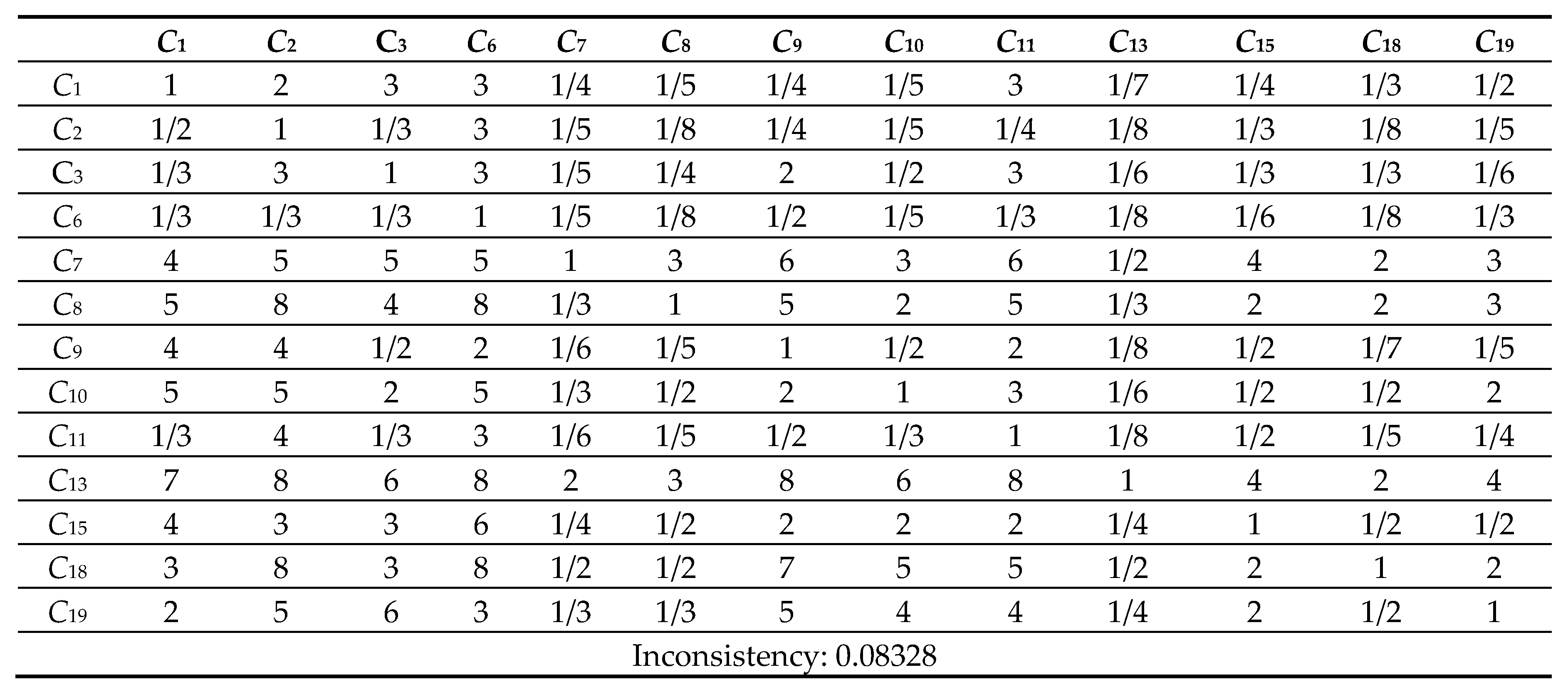
Table 10.
2 Comparison Matrix of 13 criteria with respect to criterion 2.
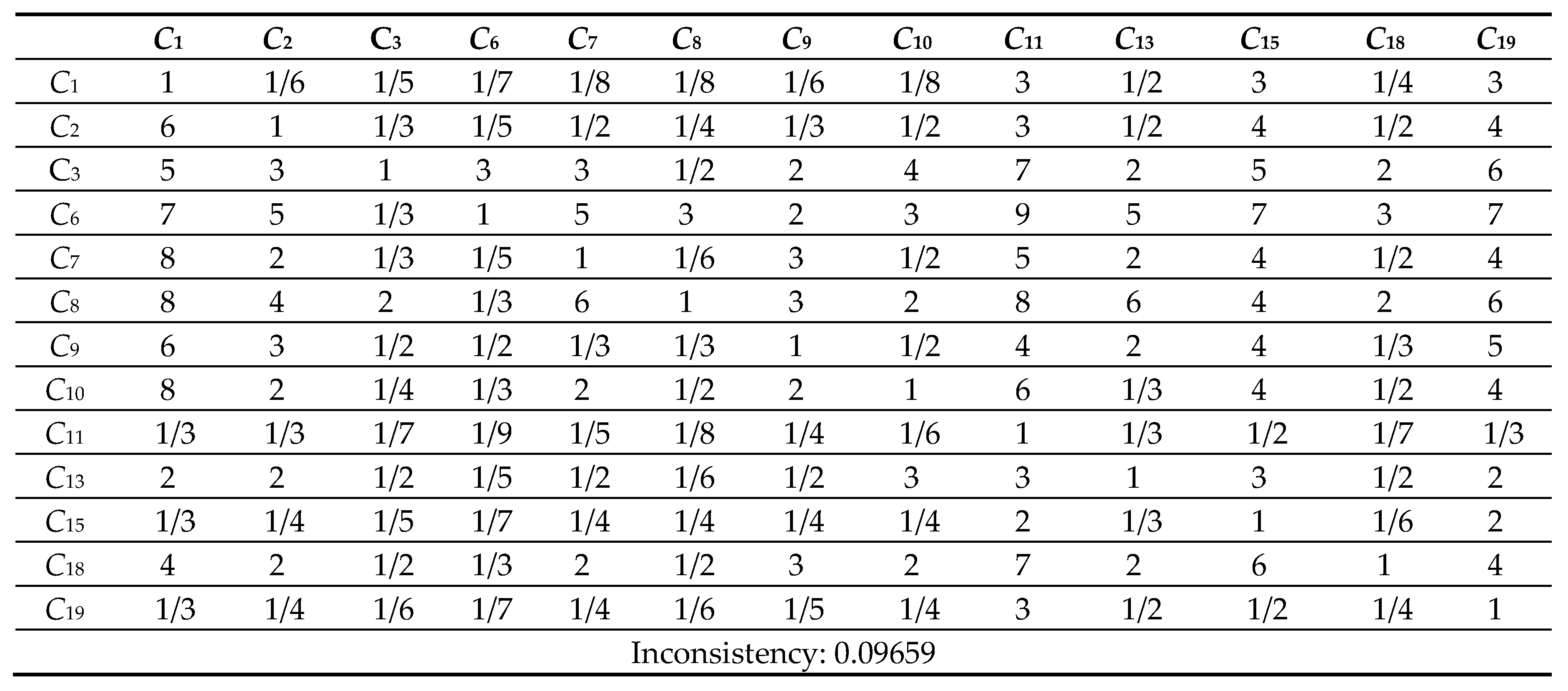
Table 10.
3 Comparison Matrix of 13 criteria with respect to criterion 3.
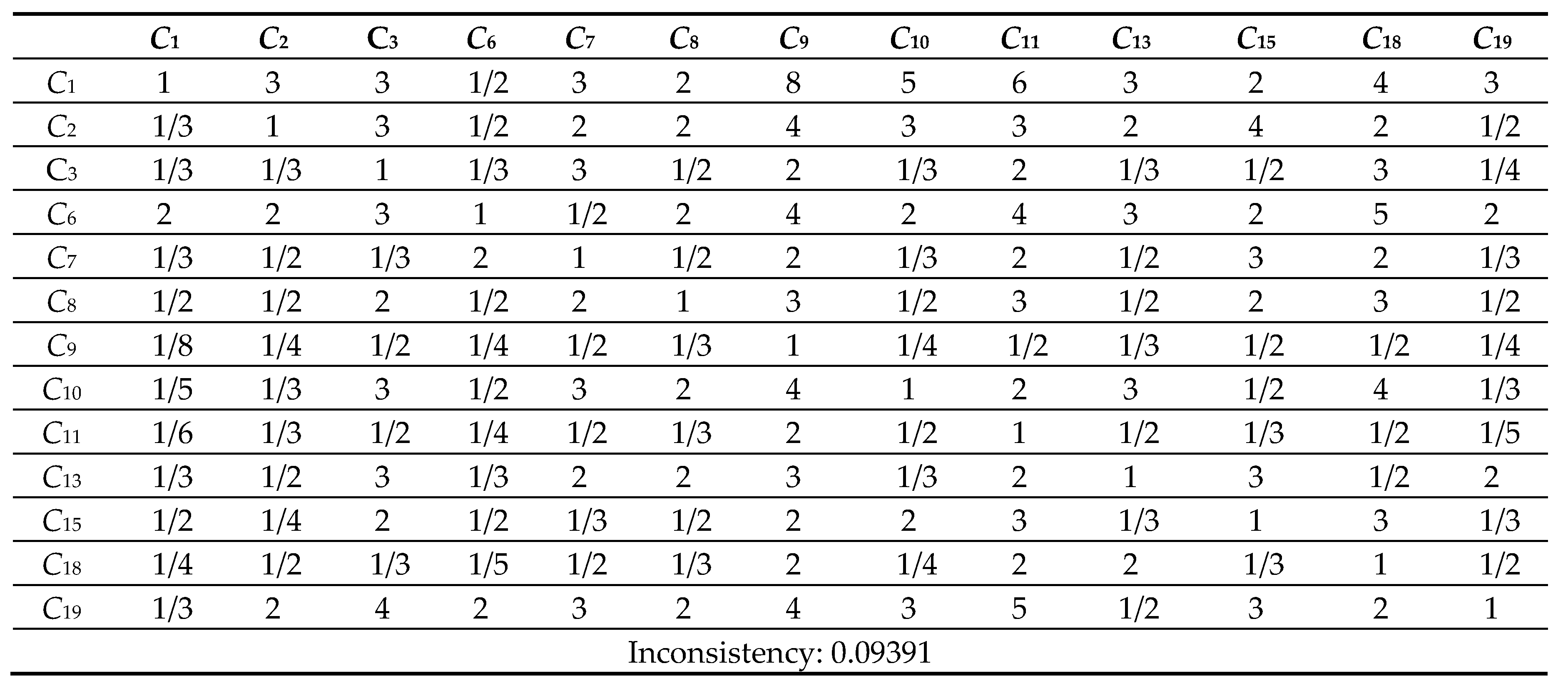
Table 10.
4 Comparison Matrix of 13 criteria with respect to criterion 6.
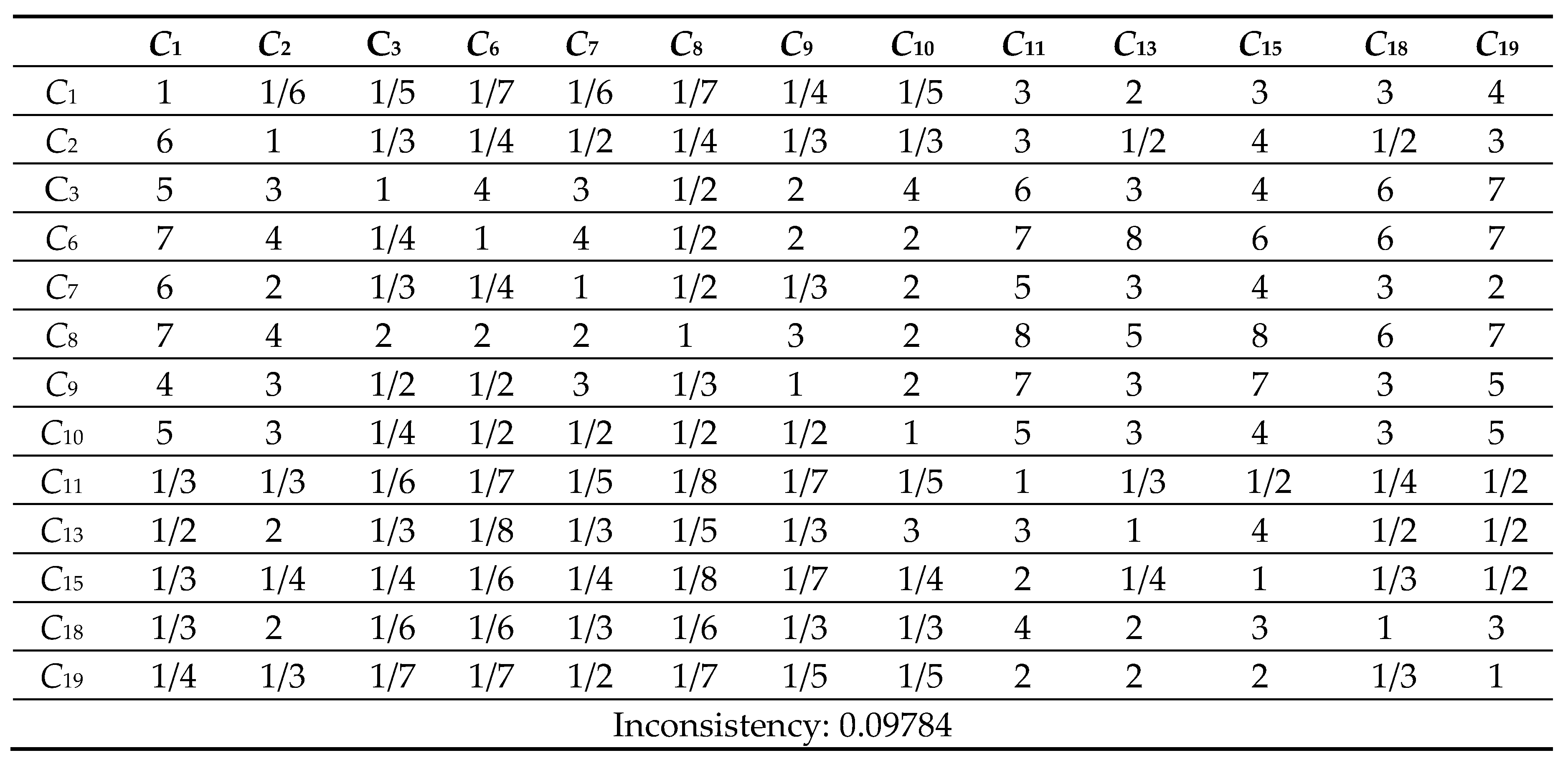
Table 10.
5 Comparison Matrix of 13 criteria with respect to criterion 7.

Table 10.
6 Comparison Matrix of 13 criteria with respect to criterion 8.
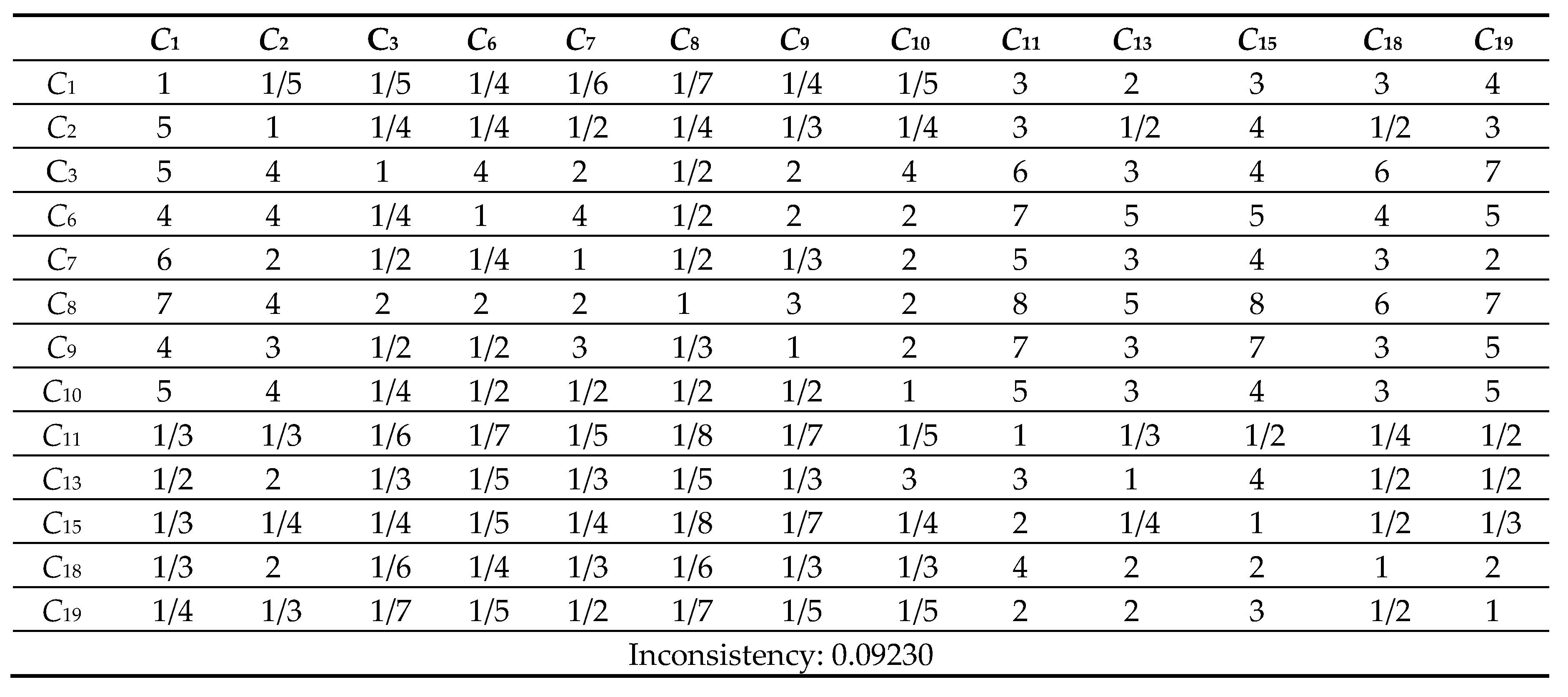
Table 10.
7 Comparison Matrix of 13 criteria with respect to criterion 9.
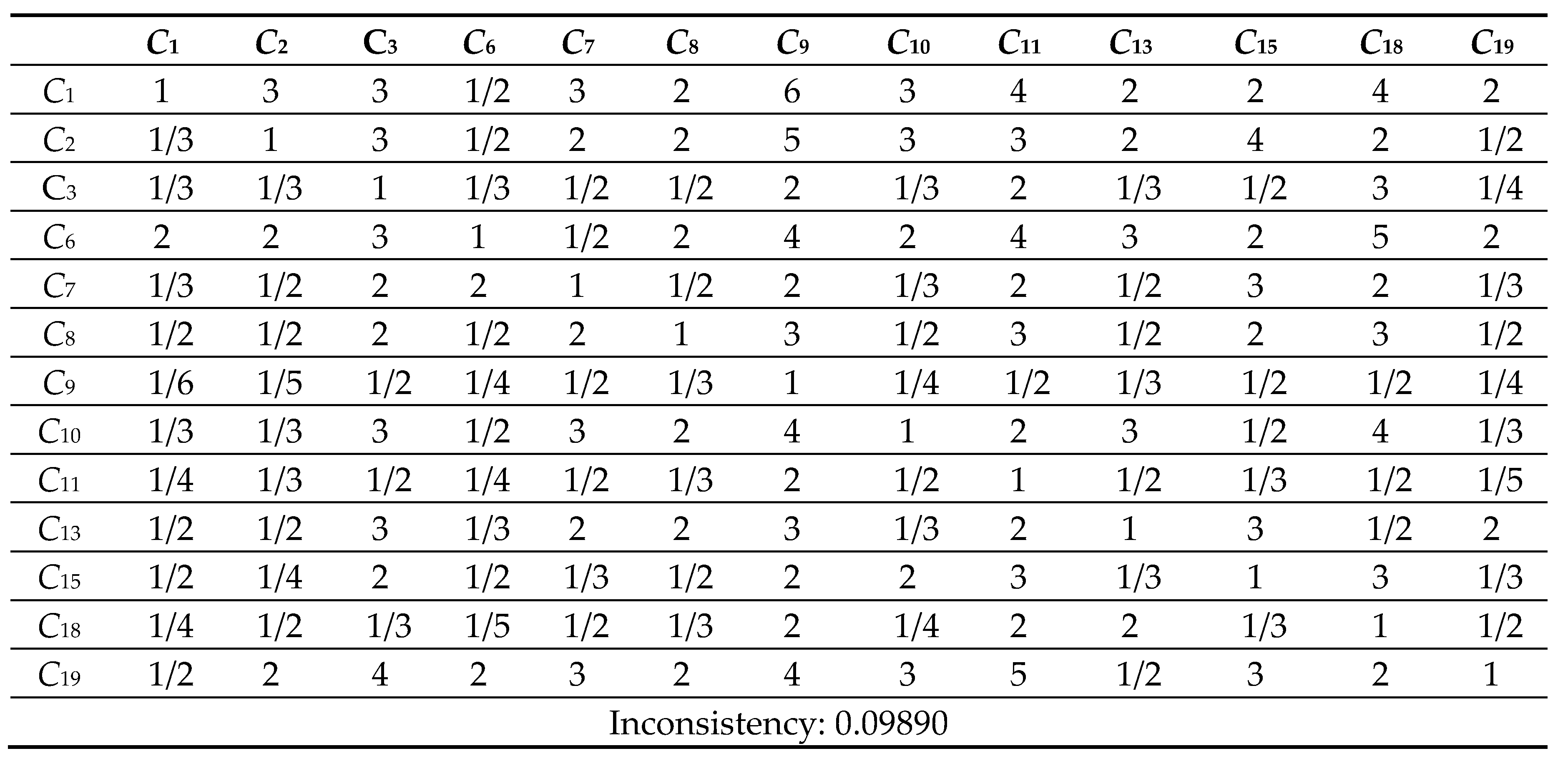
Table 10.
8 Comparison Matrix of 13 criteria with respect to criterion 10.

Table 10.
9 Comparison Matrix of 13 criteria with respect to criterion 11.
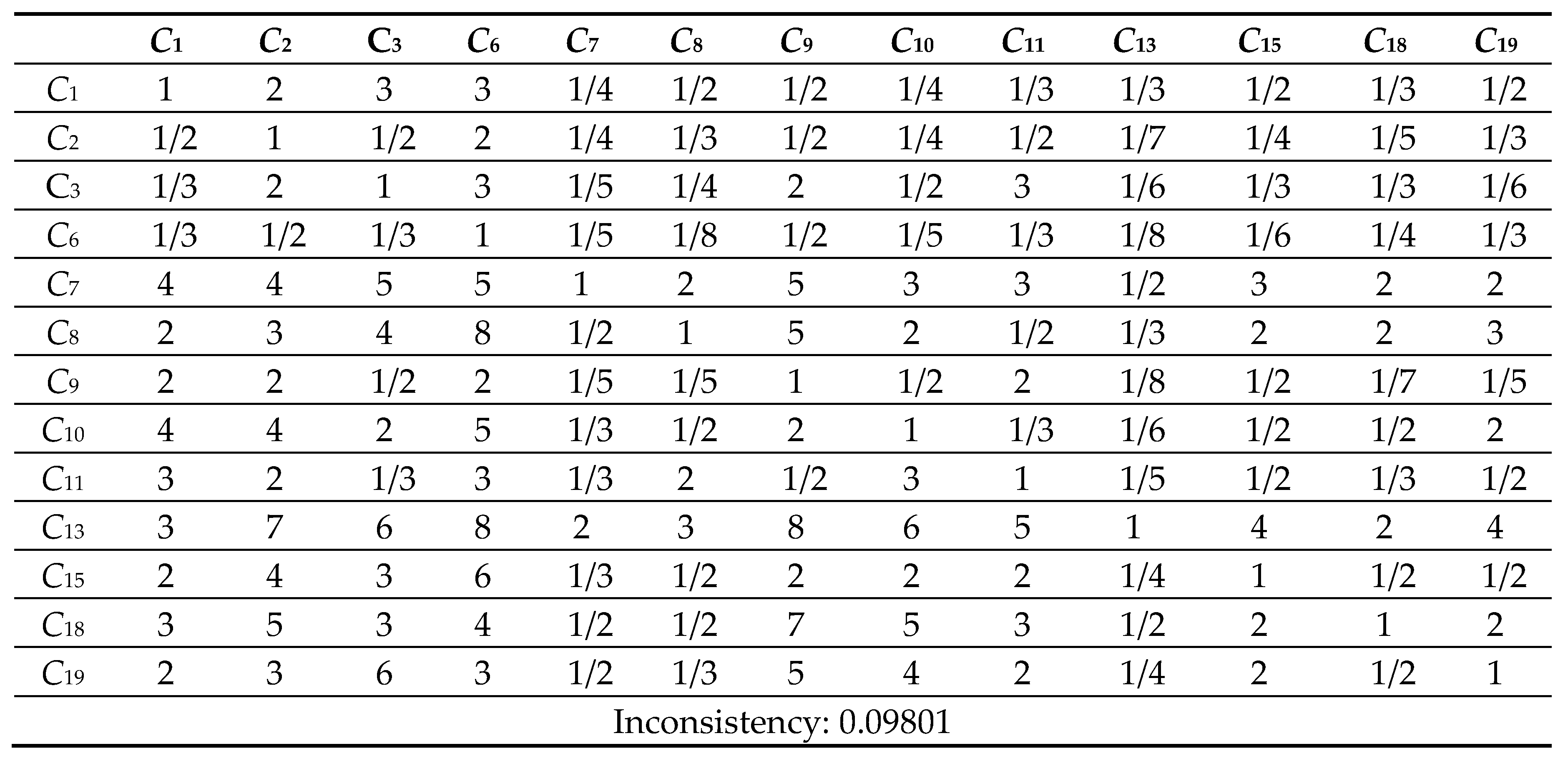
Table 10.
10 Comparison Matrix of 13 criteria with respect to criterion 13.
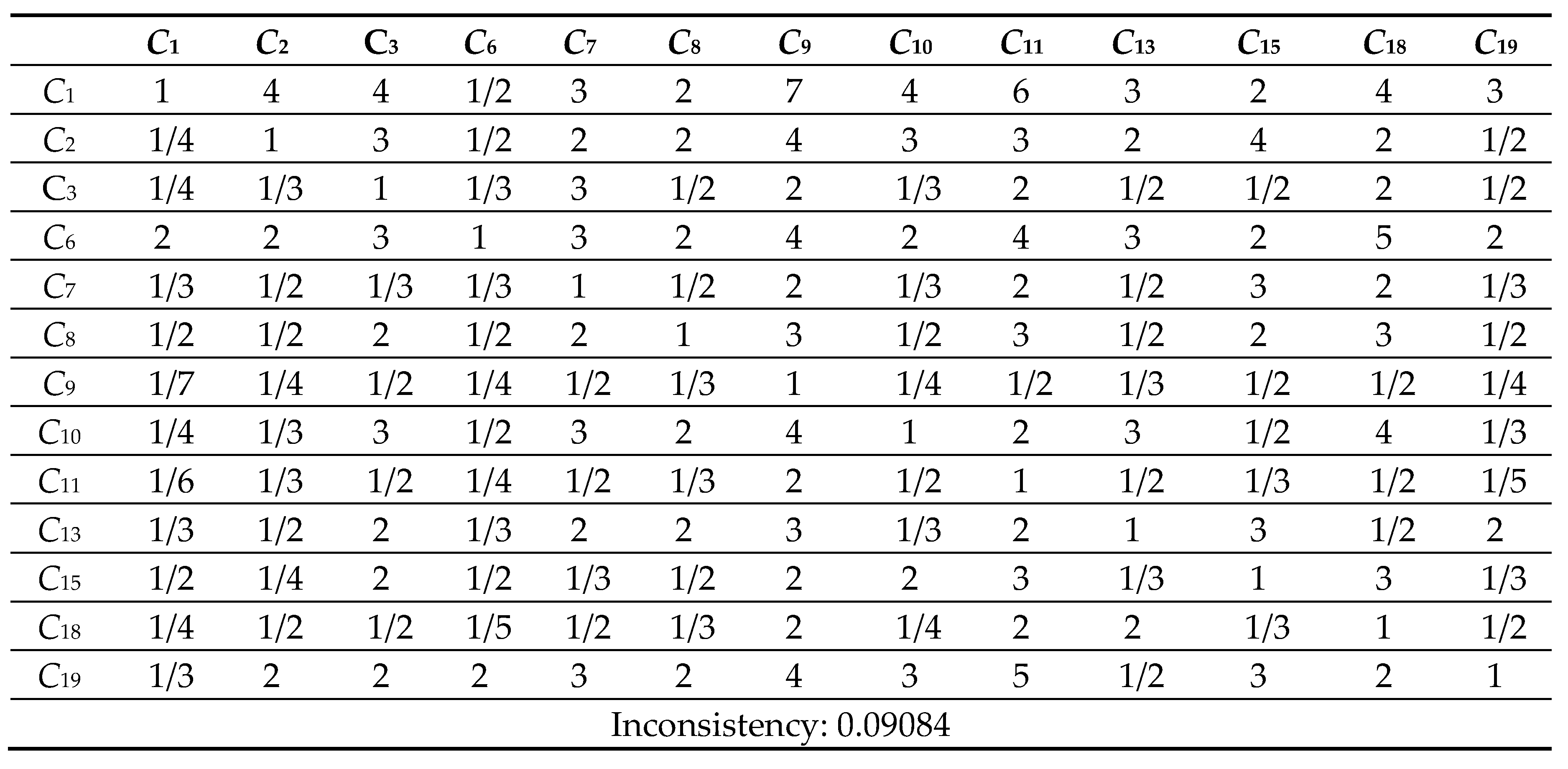
Table 10.
11 Comparison Matrix of 13 criteria with respect to criterion 15.
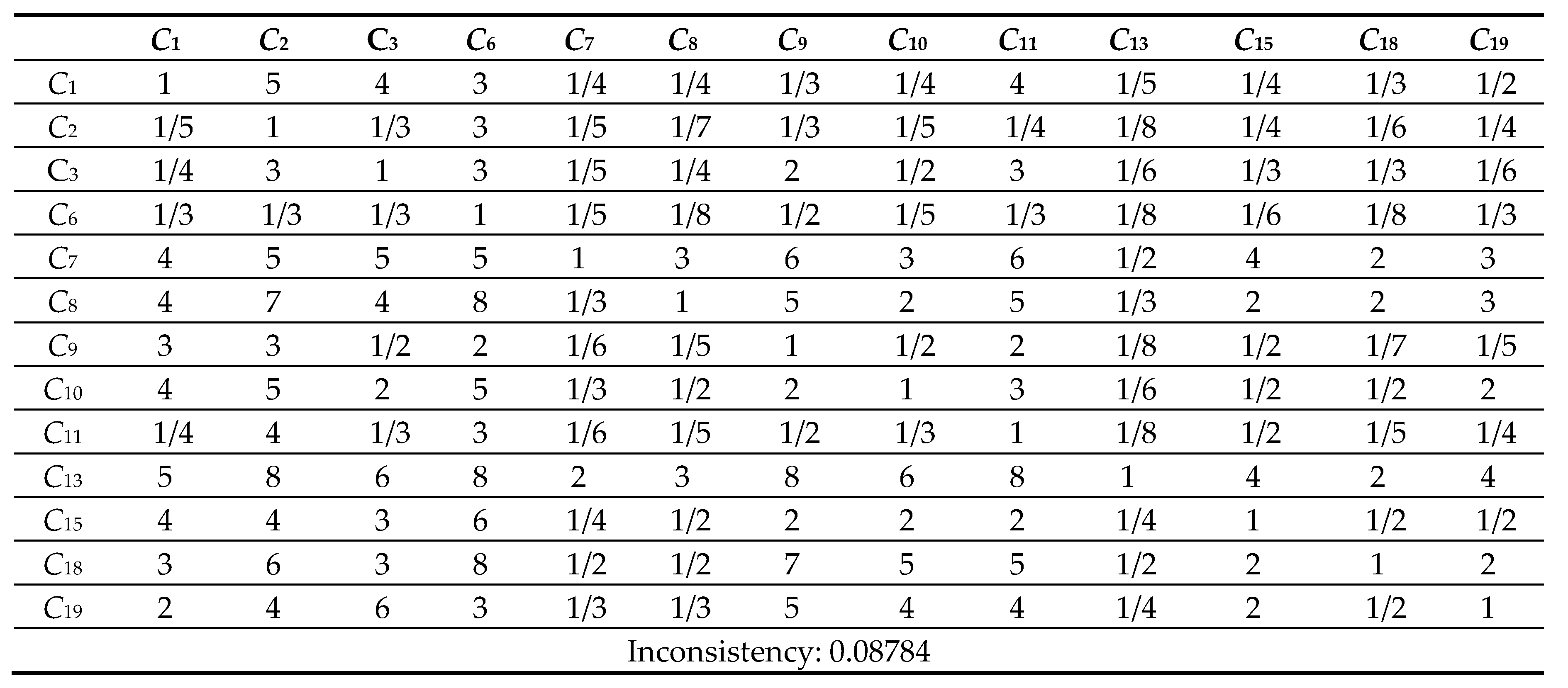
Table 10.
12 Comparison Matrix of 13 criteria with respect to criterion 18.
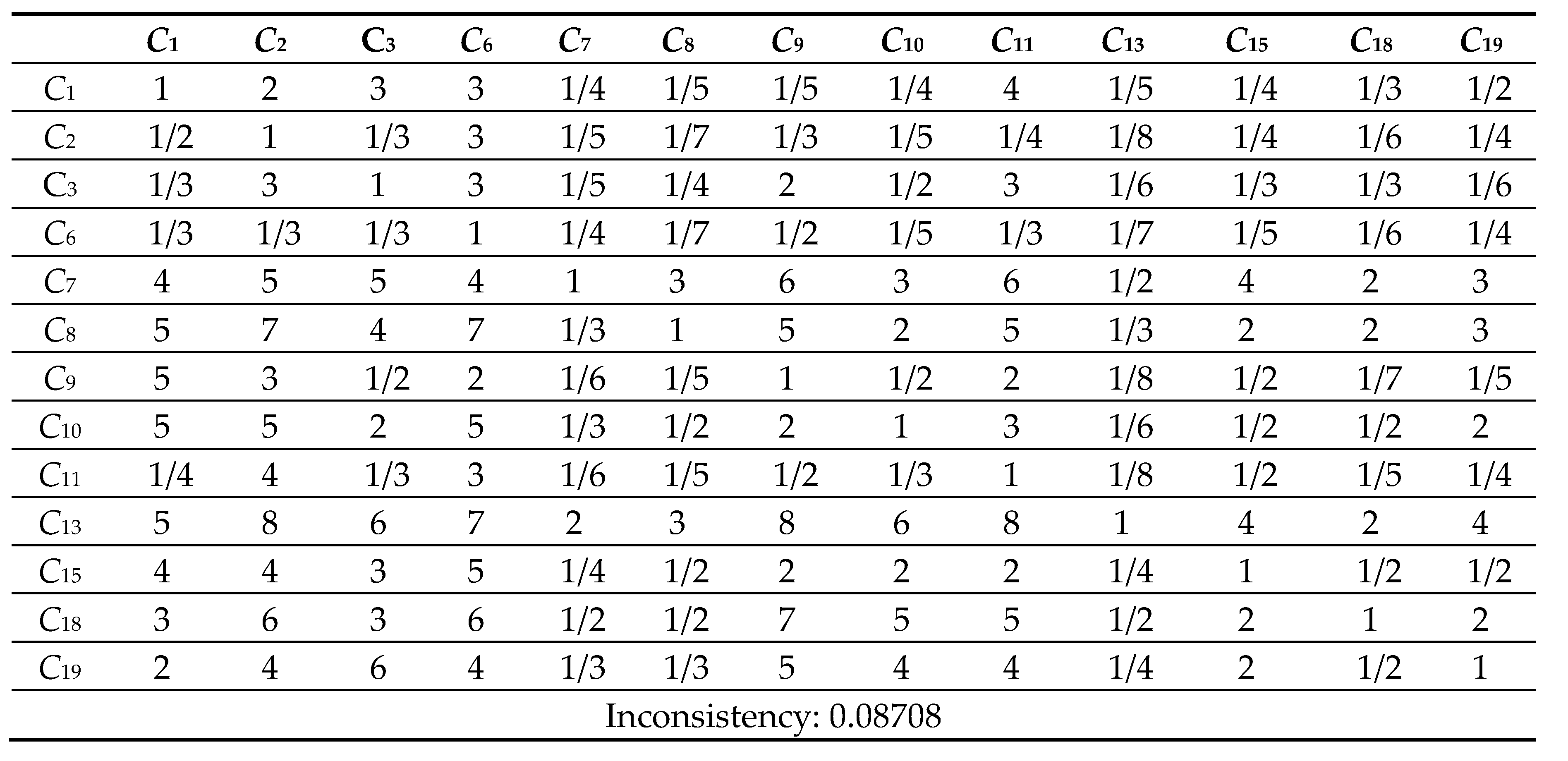
Table 10.
13 Comparison Matrix of 13 criteria with respect to criterion 19.
Appendix VII
Table 15.
Rating of Alternative Qualitative Criteria - Linguistic Values.
| DMs | Alternatives | Qualitative Criteria | |||||||||
| C6 | C7 | C8 | C9 | C10 | C11 | C12 | C13 | C14 | C15 | ||
| D1 | A1 | H | EH | H | M | H | H | VP | VH | H | H |
| A2 | VH | H | H | VH | H | H | VH | H | VH | M | |
| A3 | H | H | VH | VH | H | VH | VH | H | VH | H | |
| A4 | M | H | M | M | H | M | M | VP | EP | M | |
| D2 | A1 | H | EH | M | M | H | H | P | VH | M | H |
| A2 | H | VH | M | VH | H | H | VH | H | VH | H | |
| A3 | M | H | H | VH | H | M | VH | H | VH | M | |
| A4 | H | M | M | M | M | M | M | VP | P | M | |
| D3 | A1 | H | EH | M | H | VH | H | P | VH | M | H |
| A2 | EH | H | H | VH | H | H | VH | H | M | M | |
| A3 | VH | H | H | VH | H | P | VH | H | H | H | |
| A4 | M | M | M | M | M | H | M | P | P | M | |
| D4 | A1 | H | EH | H | H | M | M | P | VH | M | H |
| A2 | H | H | M | H | EH | P | VH | H | M | M | |
| A3 | H | VH | H | VH | H | P | VH | H | VH | M | |
| A4 | M | M | M | P | M | H | M | P | P | M | |
Appendix VIII
Table 17.
Rating of Alternative versus Quantitative Criteria.
| Alternatives | Quantitative Criteria | ||||||||
| C1 | C2 | C3 | |||||||
| A1 | 2001 | 2500 | 3000 | 101 | 150 | 200 | 3 | 4 | 5 |
| A2 | 4001 | 4500 | 5000 | 401 | 450 | 500 | 9 | 10 | 11 |
| A3 | 3001 | 3500 | 4000 | 201 | 250 | 300 | 6 | 7 | 8 |
| A4 | 1001 | 1500 | 2000 | 101 | 150 | 200 | 6 | 7 | 8 |
References
- R. Peterson, D. Valliere, Entrepreneurship and national economic growth: the European entrepreneurial deficit, European Journal of International Management, 2(4) (2008) 471-490.
- 2. P. Vandenberg, A. Hampel-Milagrosa, M. Helble, Financing of Tech Startups in Selected Asian Countries, ADBI Working Paper 1115, Tokyo: Asian Development Bank Institute (2020), https://www.adb.org/publications/financing-tech-startups-selected-asian-countries.
- E. Stam, Entrepreneurial ecosystems and regional policy: a sympathetic critique, European Planning Studies, 23(9) (2015) 1759-1769.
- C. Chang, Portfolio Company Selection Criteria: Accelerators vs Venture Capitalists, CMC Senior Theses, Paper 566 (2013), http://scholarship.claremont.edu/cmc_theses/566.
- B. Yin, J. Luo, How do accelerators select startups? Shifting decision criteria across stages, IEEE Transactions on Engineering Management, 65(4) (2018) 574-589.
- A.S. Amezcua, M.G. Grimes, S.W. Bradley, J. Wiklund, Organizational sponsorship and founding environments: A contingency view on the survival of business-incubated firms, 1994–2007, Academy of Management Journal, 56(6) (2013) 1628-1654.
- M. Lin, Z. Chen, R. Chen, H. Fujita, Evaluation of startup companies using multi-criteria decision making based on hesitant fuzzy linguistic information envelopment analysis models, International Journal of Intelligent Systems, 36(5) (2021) 2292-2322.
- C. Kahraman, S.C. Onar, B. Oztaysi, Fuzzy multi-criteria decision-making: a literature review, International journal of computational intelligence systems, 8(4) (2015) 637-666.
- J. Liu, Y. Yin, An integrated method for sustainable energy storing node optimization selection in China, Energy Conversion and Management, 199 (2019) 112049.
- I. Drori, M. Wright, Accelerators: Characteristics, trends and the new entrepreneurial ecosystem, In Accelerators, Edward Elgar Publishing (2018).
- Seed-DB., Seed-DB charts and tables, Retrieved April 19 (2023) from https://www.seed-db.com/accelerators.
- 500startups, 2021. https://500.co/accelerators/500-global-flagship-accelerator-program.
- H. Butz, M.J. Mrożewski, The Selection Process and Criteria of Impact Accelerators. An Exploratory Study, Sustainability, 13(12) (2021) 6617.
- T. Mariño-Garrido, D. García-Pérez-de-Lema, A. Duréndez, Assessment criteria for seed accelerators in entrepreneurial project selections, International Journal of Entrepreneurship and Innovation Management, 24(1) (2020) 53-72.
- Zavadskas, E. K. , Turskis, Z., & Kildienė, S. (2014). State of art surveys of overviews on MCDM/MADM methods. Technological and economic development of economy 20(1), 165-179.
- Kumar, A., Sah, B., Singh, A. R., Deng, Y., He, X., Kumar, P., & Bansal, R. C. (2017). A review of multi criteria decision making (MCDM) towards sustainable renewable energy development. Renewable and Sustainable Energy Reviews, 69, 596-609.
- Stojčić, M. , Zavadskas, E. K., Pamučar, D., Stević, Ž., & Mardani, A. (2019). Application of MCDM methods in sustainability engineering: A literature review 2008–2018. Symmetry, 11(3), 350.
- Jamwal, A. , Agrawal, R., Sharma, M., & Kumar, V. (2021). Review on multi-criteria decision analysis in sustainable manufacturing decision making. International Journal of Sustainable Engineering, 14(3), 202-225.
- Gabus, E. Fontela, World problems, an invitation to further thought within the framework of DEMATEL, Battelle Geneva Research Center, Geneva, Switzerland (1972) 1-8.
- Fontela, E. , & Gabus, A., The DEMATEL observer, DEMATEL 1976 report, Battelle Geneva Research Center, Geneva (1976).
- J. A. Moraga, L.E. Quezada, P.I. Palominos, A.M. Oddershede, H.A. Silva, A quantitative methodology to enhance a strategy map, International Journal of Production Economics, 219 (2020) 43-53.
- F. Altuntas, M.S. Gok, The effect of COVID-19 pandemic on domestic tourism: A DEMATEL method analysis on quarantine decisions, International Journal of Hospitality Management, 92 (2021) 102719.
- Wang, Y. , Qi, L., Dou, R., Shen, S., Hou, L., Liu, Y.,... & Kong, L. (2023). An accuracy-enhanced group recommendation approach based on DEMATEL. Pattern Recognition Letters, 167, 171-180.
- S.L. Si, X.Y. You, H.C. Liu, P. Zhang, DEMATEL technique: A systematic review of the state-of-the-art literature on methodologies and applications, Mathematical Problems in Engineering, (2018).
- T.L. Saaty, L.G. Vargas, The analytic network process, Decision making with the analytic network process, Springer, Boston, MA, (2013) 1-40.
- T.L Saaty, The analytic hierarchy process (AHP) for decision making, In Kobe, Japan, (1980) 1-69.
- T.L. Saaty, The analytic network process: Decision making with dependence and feedback, 2nd Ed. Pittsburgh, PA: RWS Publications (2001).
- T.L. Saaty, Theory and applications of the analytic network process: decision making with benefits, opportunities, costs, and risks, RWS publications (2005).
- D. Yu, G. Kou, Z. Xu, S. Shi, Analysis of collaboration evolution in AHP research: 1982–2018, International Journal of Information Technology & Decision Making, 20(01) (2021) 7-36.
- M. R. Galankashi, F. M. Rafiei, M. Ghezelbash, Portfolio selection: a fuzzy-ANP approach, Financial Innovation, 6(1) (2020) 1-34.
- Saputro, K. E. A. , Karlinasari, L., & Beik, I. S. (2023). Evaluation of Sustainable Rural Tourism Development with an Integrated Approach Using MDS and ANP Methods: Case Study in Ciamis, West Java, Indonesia. Sustainability 15(3), 1835.
- N. Kadoić, Characteristics of the analytic network process, a multi-criteria decision-making method, Croatian operational research review, (2018) 235-244.
- J.P. Brans, Lingenierie de la decision. Elaboration dinstruments daide a la decision. Methode PROMETHEE, In: Nadeau, R., Landry, M. (Eds.), Laide a la Decision: Nature, Instruments et Perspectives Davenir. Presses de Universite Laval, Qu ebec, Canada, (1982) 183–214.
- J. P. Brans, P. Vincke, Note-A Preference Ranking Organisation Method: (The PROMETHEE Method for Multiple Criteria Decision-Making), Management science, 31(6) (1985) 647-656.
- J. P. Brans, The space of freedom of the decision maker modelling the human brain, European Journal of Operational Research, 92(3) (1996) 593-602.
- M. Abedi, S.A. Torabi, G.H. Norouzi, M. Hamzeh, G.R. Elyasi, PROMETHEE II: a knowledge-driven method for copper exploration, Computers & Geosciences, 46 (2012) 255-263.
- H. Jiang, J. Zhan, D. Chen, PROMETHEE II method based on variable precision fuzzy rough sets with fuzzy neighborhoods, Artificial Intelligence Review, 54(2) (2021) 1281-1319.
- Hua, Z. , & Jing, X. (2023). A generalized Shapley index-based interval-valued Pythagorean fuzzy PROMETHEE method for group decision-making. Soft Computing, 1-24.
- E. Khorasaninejad, A. Fetanat, H. Hajabdollahi, Prime mover selection in thermal power plant integrated with organic Rankine cycle for waste heat recovery using a novel multi criteria decision making approach, Applied Thermal Engineering, 102 (2016) 1262-1279.
- K. Govindan, D. Kannan, M. Shankar, Evaluation of green manufacturing practices using a hybrid MCDM model combining DANP with PROMETHEE, International Journal of Production Research, 53(21) (2015) 6344-6371.
- W. Torbacki, A Hybrid MCDM Model Combining DANP and PROMETHEE II Methods for the Assessment of Cybersecurity in Industry 4.0, Sustainability, 13(16) (2021) 8833.
- L.A. Zadeh, Fuzzy Sets. Information and Control, 8(1) (1965).
- Al-Tahan, M. , Hoskova-Mayerova, S., Al-Kaseasbeh, S., & Tahhan, S. A. (2023). Linear Diophantine Fuzzy Subspaces of a Vector Space. Mathematics, 11(3), 503.
- Ardil, C. (2023). Aircraft Supplier Selection using Multiple Criteria Group Decision Making Process with Proximity Measure Method for Determinate Fuzzy Set Ranking Analysis. International Journal of Industrial and Systems Engineering 17(3), 127-135.
- Karmaker, C. L. , Al Aziz, R., Palit, T., & Bari, A. M. (2023). Analyzing supply chain risk factors in the small and medium enterprises under fuzzy environment: Implications towards sustainability for emerging economies. Sustainable Technology and Entrepreneurship, 2(1), 100032.
- C. Kahraman, B. Öztayşi, S. Çevik Onar, A comprehensive literature review of 50 years of fuzzy set theory, International Journal of Computational Intelligence Systems, 9(sup1) (2016) 3-24.
- R. Jain, (Decision-making in the presence of fuzzy variables, IEEE Trans. Syst. Man and Cybernet, SMC-6(10) 1976) 698–703.
- Dubois, H. Prade, Ranking fuzzy numbers in the setting of possibility theory, Information sciences, 30(3) (1983) 183-224.
- S.H. Chen, Ranking fuzzy numbers with maximizing set and minimizing set, Fuzzy sets and Systems, 17(2) (1985) 113-129.
- P. Fortemps, M. Roubens, Ranking and defuzzification methods based on area compensation, Fuzzy sets and systems, 82(3) (1996) 319-330.
- Y. Deng, Z. Zhenfu, L.Qi, Ranking fuzzy numbers with an area method using radius of gyration, Computers & Mathematics with Applications, 51(6-7) (2006) 1127-1136.
- Z.X. Wang, Y.J. Liu, Z.P. Fan, B. Feng, Ranking L–R fuzzy number based on deviation degree, Information Sciences, 179(13) (2009) 2070-2077.
- S.M. Chen, J.H. Chen, Fuzzy risk analysis based on ranking generalized fuzzy numbers with different heights and different spreads, Expert Systems with Applications, 36 (2009) 6833-6842.
- H.T. Nguyen, T.C. Chu, Using a fuzzy multiple criteria decision-making method to evaluate personal diversity perception to work in a diverse workgroup, Journal of Intelligent & Fuzzy Systems, 41 (2021) 1407-1428.
- .M. Wang, Y. Luo, Area ranking of fuzzy numbers based on positive and negative ideal points, Computers & Mathematics with Applications, 58(9) (2009) 1769-1779.
- B. Asady, The revised method of ranking LR fuzzy number based on deviation degree, Expert Systems with Applications, 37(7) (2010) 5056-5060.
- A.M. Nejad, M. Mashinchi, Ranking fuzzy numbers based on the areas on the left and the right sides of fuzzy number, Computers & Mathematics with Applications, 61(2) (2011) 431-442.
- V.F. Yu, H.T.X. Chi, C.W. Shen, Ranking fuzzy numbers based on epsilon-deviation degree, Applied Soft Computing, 13(8) (2013) 3621-3627.
- R. Chutia, Ranking of fuzzy numbers by using value and angle in the epsilon-deviation degree method, Applied Soft Computing, 60 (2017) 706-721.
- R. Ghasemi, M. Nikfar, E. Roghanian, A revision on area ranking and deviation degree methods of ranking fuzzy numbers, Scientia Iranica, 22(3) (2015) 1142-1154.
- T.C. Chu, H.T. Nguyen, Ranking alternatives with relative maximizing and minimizing sets in a fuzzy MCDM model, International Journal of Fuzzy Systems, 21(4) (2019) 1170-1186.
- A. Kaufman, M.M. Gupta, Introduction to fuzzy arithmetic, New York: Van Nostrand Reinhold Company (1991).
- L.A. Zadeh, Outline of a new approach to the analysis of complex systems and decision processes, IEEE Transactions on systems, Man, and Cybernetics, (1) (1973) 28-44.
- C.H. Yeh, Y.L. Kuo, Evaluating passenger services of Asia-Pacific international airports, Transportation Research Part E: Logistics and Transportation Review, 39(1) (2003) 35-48.
- C.Y. Huang, J.Z. Shyu, G.H. Tzeng, Reconfiguring the innovation policy portfolios for Taiwan’s SIP Mall industry, Technovation, 27(12) (2007) 744-765.
- .H. Tzeng, C.H. Chiang, C.W. Li, Evaluating intertwined effects in e-learning programs: A novel hybrid MCDM model based on factor analysis and DEMATEL, Expert systems with Applications, 32(4) (2007) 1028-1044.
- K.F. Chien, Z.H. Wu, S.C. Huang, Identifying and assessing critical risk factors for BIM projects: Empirical study, Automation in construction, 45 (2014) 1-15.
- W.R. Lin, Y.H. Wang, Y.M. Hung, Analyzing the factors influencing adoption intention of internet banking: Applying DEMATEL-ANP-SEM approach, Plos one, 15(2) (2020) e0227852.
- H. Farman, H. Javed, B. Jan, J. Ahmad, S. Ali, F.N. Khalil, M. Khan, Analytical network process based optimum cluster head selection in wireless sensor network, PLoS One, 12(7) (2017) e0180848.
- J. Geldermann, T. Spengler, O. Rentz, Fuzzy outranking for environmental assessment. Case study: iron and steel making industry, Fuzzy sets and systems, 115(1) (2000) 45-65.
- S.R. Maity, S. Chakraborty, Tool steel material selection using PROMETHEE II method, The International Journal of Advanced Manufacturing Technology, 78(9-12) (2015) 1537-1547.
Figure 1.
Spread area-based RMMS ranking method.
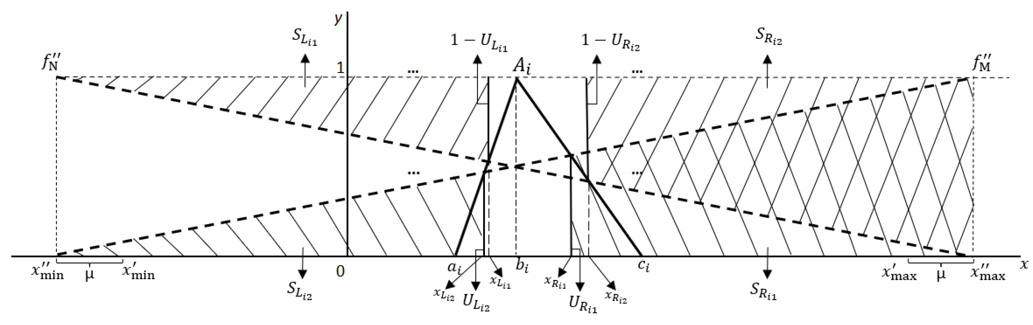
Figure 3.
Causal Diagram.
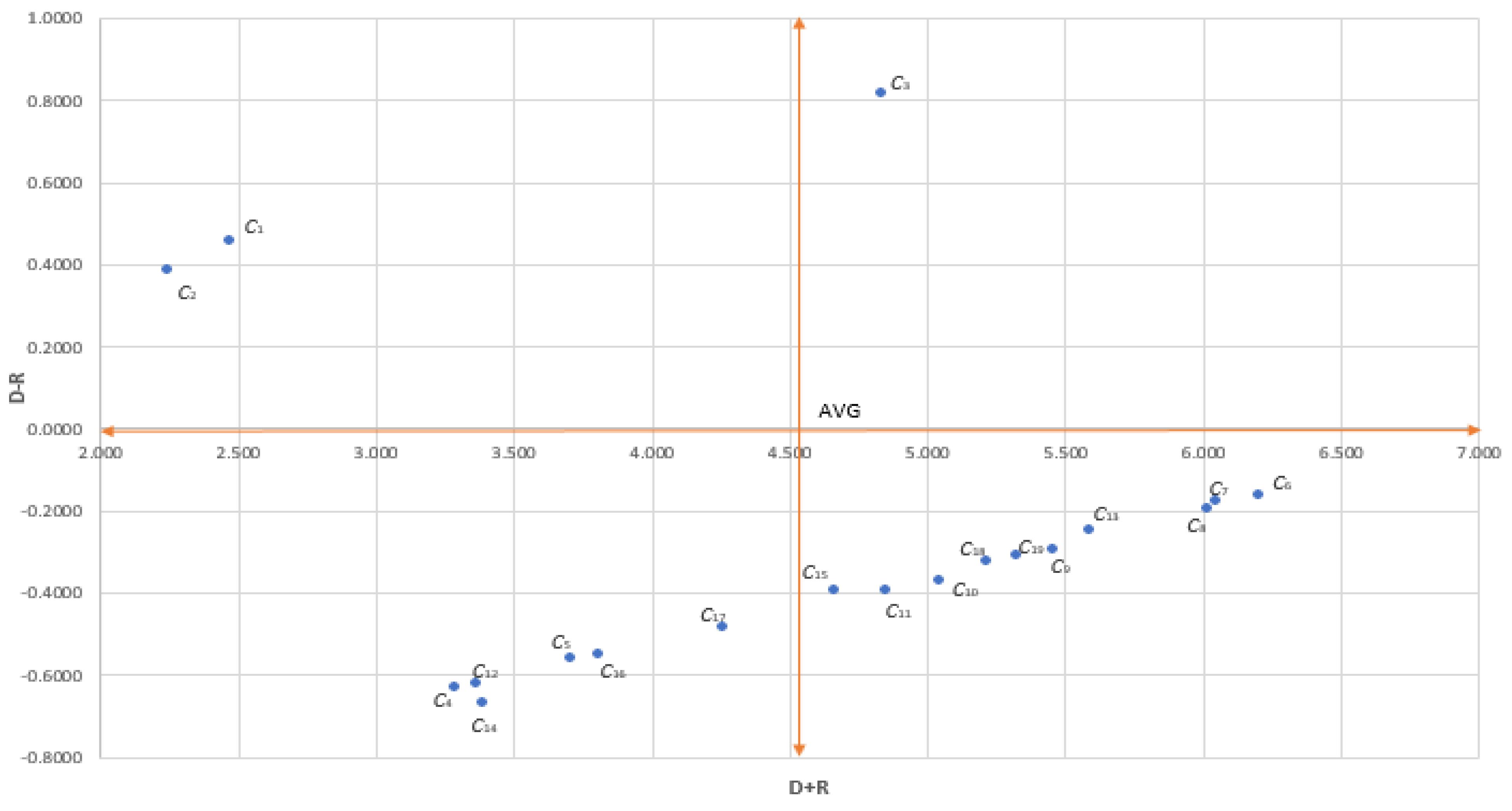
Table 1.
Random Index.
| Order | 1 | 2 | 3 | 4 | 5 | 6 | 7 | 8 | 9 | 10 |
|---|---|---|---|---|---|---|---|---|---|---|
| R.I | 0 | 0 | 0.52 | 0.89 | 1.11 | 1.25 | 1.35 | 1.40 | 1.45 | 1.49 |
Table 2.
Modified comparison based on Examples 2, 3, and 4 from Nejad and Mashinchi’s [57].
Table 2.
Modified comparison based on Examples 2, 3, and 4 from Nejad and Mashinchi’s [57].
| Situations | Methods | Results | Results after adding new FNs | |
|---|---|---|---|---|
| (1) | (1.1) | (1.2) | ||
| Wang et al. | ||||
| Nejad and Mashinchi | ||||
| Proposed method | ||||
| (2) | (2.1) | (2.2) | ||
| Wang et al. | ||||
| Nejad and Mashinchi | ||||
| Proposed method | ||||
| (3) | (3.1) | (3.2) | ||
| Wang et al. | ||||
| Nejad and Mashinchi | ||||
| Proposed method | ||||
| Situations | Methods | Results | Results after adding new FNs | |
| (1) | (1.1) | (1.2) | ||
| Wang et al. | ||||
| Nejad and Mashinchi | ||||
| Proposed method | ||||
| (2) | (2.1) | (2.2) | ||
| Wang et al. | ||||
| Nejad and Mashinchi | ||||
| Proposed method | ||||
| (3) | (3.1) | (3.2) | ||
| Wang et al. | ||||
| Nejad and Mashinchi | ||||
| Proposed method | ||||
Table 4.
Numerical comparison with Chu and Nguyen [61].
Table 4.
Numerical comparison with Chu and Nguyen [61].
| Situations | Methods | Results | Results after adding new FNs | |
| (1) | (1.1) | (1.2) | ||
| Chu and Nguyen | ||||
| Proposed method | ||||
| (2) | (2.1) | (2.2) | ||
| Chu and Nguyen | ||||
| Proposed method | ||||
Table 9.
Prominence and Relation value of criteria.
| D | R | D + R | D – R | |
| C1 | 1.4660 | 1.0098 | 2.476 | 0.4562 |
| C2 | 1.3166 | 0.9326 | 2.249 | 0.3840 |
| C3 | 2.8245 | 2.0101 | 4.835 | 0.8144 |
| C4 | 1.3291 | 1.9605 | 3.290 | -0.6314 |
| C5 | 1.5740 | 2.1332 | 3.707 | -0.5593 |
| C6 | 3.0201 | 3.1850 | 6.205 | -0.1649 |
| C7 | 2.9359 | 3.1138 | 6.050 | -0.1778 |
| C8 | 2.9104 | 3.1088 | 6.019 | -0.1985 |
| C9 | 2.5804 | 2.8768 | 5.457 | -0.2964 |
| C10 | 2.3358 | 2.7069 | 5.043 | -0.3711 |
| C11 | 2.2284 | 2.6253 | 4.854 | -0.3969 |
| C12 | 1.3718 | 1.9929 | 3.365 | -0.6211 |
| C13 | 2.6701 | 2.9201 | 5.590 | -0.2500 |
| C14 | 1.3602 | 2.0277 | 3.388 | -0.6675 |
| C15 | 2.1349 | 2.5318 | 4.667 | -0.3969 |
| C16 | 1.6294 | 2.1784 | 3.808 | -0.5490 |
| C17 | 1.8855 | 2.3726 | 4.258 | -0.4871 |
| C18 | 2.4492 | 2.7714 | 5.221 | -0.3222 |
| C19 | 2.5088 | 2.8181 | 5.327 | -0.3093 |
| Average | 4.516 |
Table 16.
The average ratings of the alternatives over qualitative criteria.
| Cn | Average rating | |||||||||||
| A1 | A2 | A3 | A4 | |||||||||
| (aj1, bj1, cj1) | (aj2, bj2, cj2) | (aj3, bj3, cj3) | (aj4, bj4, cj4) | |||||||||
| C6 | 0.500 | 0.650 | 0.750 | 0.600 | 0.750 | 0.850 | 0.500 | 0.650 | 0.763 | 0.388 | 0.538 | 0.675 |
| C7 | 0.750 | 0.900 | 1.000 | 0.538 | 0.688 | 0.788 | 0.538 | 0.688 | 0.788 | 0.388 | 0.538 | 0.675 |
| C8 | 0.425 | 0.575 | 0.700 | 0.425 | 0.575 | 0.700 | 0.538 | 0.688 | 0.788 | 0.350 | 0.500 | 0.650 |
| C9 | 0.425 | 0.575 | 0.700 | 0.613 | 0.763 | 0.863 | 0.650 | 0.800 | 0.900 | 0.325 | 0.463 | 0.613 |
| C10 | 0.500 | 0.650 | 0.763 | 0.563 | 0.713 | 0.813 | 0.500 | 0.650 | 0.750 | 0.388 | 0.538 | 0.675 |
| C11 | 0.463 | 0.613 | 0.725 | 0.438 | 0.575 | 0.688 | 0.375 | 0.500 | 0.638 | 0.425 | 0.575 | 0.700 |
| C13 | 0.213 | 0.313 | 0.463 | 0.650 | 0.800 | 0.900 | 0.650 | 0.800 | 0.900 | 0.350 | 0.500 | 0.650 |
| C15 | 0.213 | 0.313 | 0.463 | 0.650 | 0.800 | 0.900 | 0.650 | 0.800 | 0.900 | 0.350 | 0.500 | 0.650 |
| C18 | 0.388 | 0.538 | 0.675 | 0.500 | 0.650 | 0.775 | 0.613 | 0.763 | 0.863 | 0.188 | 0.288 | 0.438 |
| C19 | 0.500 | 0.650 | 0.750 | 0.388 | 0.538 | 0.675 | 0.425 | 0.575 | 0.700 | 0.350 | 0.500 | 0.650 |
Table 18.
The average ratings of the alternatives over quantitative criteria.
| Cn | Average rating | |||||||||||
| A1 | A2 | A3 | A4 | |||||||||
| (al1, bl1, cl1) | (al2, bl2, cl2) | (al3, bl3, cl3) | (al4, bl4, cl4) | |||||||||
| C1 | 0.250 | 0.375 | 0.500 | 0.750 | 0.875 | 1.000 | 0.500 | 0.625 | 0.750 | 0.000 | 0.125 | 0.250 |
| C2 | 0.752 | 0.877 | 1.000 | 0.000 | 0.125 | 0.248 | 0.501 | 0.627 | 0.749 | 0.750 | 0.875 | 1.000 |
| C3 | 0.000 | 0.125 | 0.250 | 0.750 | 0.875 | 1.000 | 0.375 | 0.500 | 0.625 | 0.375 | 0.500 | 0.625 |
Table 19.
Confidence level µ from DMs.
| A1 | A2 | A3 | A4 | A1 | A2 | A3 | A4 | µ | ||
| D1 | 0.6 | 0.8 | 0.7 | 0.6 | D3 | 0.7 | 0.7 | 0.8 | 0.5 | 0.6625 |
| D2 | 0.6 | 0.8 | 0.7 | 0.5 | D4 | 0.5 | 0.8 | 0.7 | 0.6 |
Table 20.
The aggregated fuzzy TNs preference.
| A1 | A2 | A3 | A4 | |||||||||
| A1 | - | - | - | 0.0321 | 0.0479 | 0.0637 | 0.0002 | 0.0160 | 0.0318 | 0.0164 | 0.0771 | 0.1301 |
| A2 | 0.0863 | 0.1594 | 0.1998 | - | - | - | 0.0118 | 0.0574 | 0.1030 | 0.0628 | 0.1825 | 0.2857 |
| A3 | 0.0289 | 0.1020 | 0.1659 | 0.0161 | 0.0320 | 0.0478 | - | - | - | 0.0373 | 0.1336 | 0.2118 |
| A4 | 0.0117 | 0.0352 | 0.0587 | 0.0321 | 0.0479 | 0.0637 | 0.0002 | 0.0160 | 0.0318 | - | - | - |
Table 21.
The fuzzy TNs net outranking flow for each alternative.
| ϕ+ | ϕ- | ϕ | |||||||
| A1 | 0.0162 | 0.0470 | 0.0752 | 0.0423 | 0.0989 | 0.1415 | -0.1253 | -0.0519 | 0.0329 |
| A2 | 0.0536 | 0.1331 | 0.1962 | 0.0268 | 0.0426 | 0.0584 | -0.0048 | 0.0905 | 0.1694 |
| A3 | 0.0275 | 0.0892 | 0.1418 | 0.0040 | 0.0298 | 0.0555 | -0.0281 | 0.0594 | 0.1378 |
| A4 | 0.0147 | 0.0330 | 0.0514 | 0.0388 | 0.1310 | 0.2092 | -0.1945 | -0.0980 | 0.0126 |
Table 22.
Deffuzication and ranking of the alternatives.
| ϕ | SL1 | SL2 | SR1 | SR2 | V(Ai) | Ranking | |||
| A1 | -0.1253 | -0.0519 | 0.0329 | 0.9364 | 0.1733 | 0.6221 | 0.6364 | -0.0519 | 3 |
| A2 | -0.0048 | 0.0905 | 0.1694 | 1.1217 | 0.2415 | 0.6852 | 0.4956 | 0.0905 | 1 |
| A3 | -0.0281 | 0.0594 | 0.1378 | 1.0830 | 0.2263 | 0.6719 | 0.5262 | 0.0594 | 2 |
| A4 | -0.1945 | -0.0980 | 0.0126 | 0.8599 | 0.1462 | 0.6058 | 0.6724 | -0.0980 | 4 |
Disclaimer/Publisher’s Note: The statements, opinions and data contained in all publications are solely those of the individual author(s) and contributor(s) and not of MDPI and/or the editor(s). MDPI and/or the editor(s) disclaim responsibility for any injury to people or property resulting from any ideas, methods, instructions or products referred to in the content. |
© 2023 by the authors. Licensee MDPI, Basel, Switzerland. This article is an open access article distributed under the terms and conditions of the Creative Commons Attribution (CC BY) license (http://creativecommons.org/licenses/by/4.0/).
Copyright: This open access article is published under a Creative Commons CC BY 4.0 license, which permit the free download, distribution, and reuse, provided that the author and preprint are cited in any reuse.


