
Submitted:
20 April 2023
Posted:
21 April 2023
You are already at the latest version
Abstract
The battery energy storage systems (BESS) are most promising solution for increasing efficiency and flexibility of distribution networks (DNs) with significant penetration level of photovoltaic (PV) systems. There are various issues related to the optimal operation of DNs with integrated PV sys-tems and BESS that need to be addressed to maximize DN performance. This paper deals with the day-ahead optimal active-reactive power dispatching in unbalanced DNs with integrated sin-gle-phase PV generation and BESSs. The objectives are the minimization of cost for electricity, en-ergy losses in the DN and voltage unbalance at three-phase load buses by optimal managing of active and reactive power flows. To solve this highly constrained nonlinear optimization problem, a hybrid particle swarm optimization with sigmoid-based acceleration coefficients (PSOS) and cha-otic gravitational search algorithm (CGSA), called PSOS-CGSA algorithm, is proposed. A scenario based approach encompassing the Monte Carlo simulation (MCS) method with the simultaneous backward reduction algorithm is used for the probabilistic assessment of the uncertainty of PV generation and power of loads. The effectiveness of the proposed procedure is evaluated through the series test cases in a modified IEEE 13-bus feeder.
Keywords:
distribution network
; PV generation
; battery energy storage
; optimal power dispatch
; uncertainty
; scenario reduction
1. Introduction
In light of the recent energy crisis, in the midst of the energy transition towards carbon free power systems, the advantages of renewable energy sources (RESs), such as photovoltaic (PV) generators whose growth has been exponential over the last twenty years [1], position them in the center of related policies. However, they suffer from variability and stochasticity of the output power which is their main drawback [2] and a challenge attracting the interest of research community. A promising approach towards a more flexible use of PV sources is their combination with battery energy storage systems (BESSs) to fully exploit the potential of PV units integrated into distribution networks (DNs) [3].
In the last few years, a number of authors have addressed the issues of the optimal power dispatch in DNs with integrated BESSs. These studies have been focused on several main aspects such as: modeling BESSs, defining the BESS function in DNs, i.e. objective functions of the optimization problem, defining control variables, dependent variables and technical constraints, as well as the choice of solution methods.
The BESS is a combination of a voltage source converter and a battery pack, such that the active and reactive power can be controlled independently [4,5,6,7,8,9]. In most research articles, BESS are modeled as a set of equations defining that the stored energy at any given time segment is a function of the stored energy, and charge/discharge power at the previous time segment. Internal losses of BESS are accounted for through the charge/discharge efficiency coefficients or functions. The limits of the reactive power output to be provided by the BESS are also defined in these models.
Depending on the function that the BESS performs in the DN, the objectives for the optimal power dispatch can be summarized in three groups: technical objectives, financial objectives, and multi-objectives. Financial objectives can be related to the maximization of revenues of a RES-BESS based hybrid power plant [10], the reduction in the energy cost from the source grid [11,12], as well as the minimization of distributed generators dispatch costs [13], power generation costs and load shedding costs [5]. Technical objectives are the base objectives and include the static voltage stability improvement [6], the transient voltage stability enhancement [8], the energy loss minimization [9], the voltage fluctuation mitigation [14], and minimization of the voltage deviations at load buses [15]. Researchers often adopt multi-objective functions with different combinations of financial and technical objectives, such as the simultaneous maximization of the total yield from the RES and minimization of the total costs of the energy loss in DNs [4], the simultaneous minimization of the power exchange cost between the DN and transmission network and the penalty cost of the voltage deviation in the DN [7].
In its most general mathematical formulation, the optimal power dispatch in DNs with integrated RES and BESS is a non-linear, non-convex, large-scale, dynamic optimization problem with constraints. There are two approaches to solving it, namely classical optimization methods and metaheuristic methods.
The non-linear optimization models are implemented in the GAMS environment and solved using CONOPT3 solver [4], CPLEX solver [5], and KNITRO solver [11]. The big M method is used in [7] to transform the model into a mixed-integer linear programming problem and solved using a commercial software. The interior-point solver fmincon in MATLAB [9] and the simplex solver through docplex python library [10] are also suggested for the optimal power flow in DNs with the BESS, whereas Giuntoli et al. [13] used the CaADdi framework for interfacing with the IPOPT solver for nonlinear programming. In recent research, some population-based methods, such as PSO, have been proposed to find the optimal power dispatch solution in the DN with the BESS [6,15].
This paper is an expanded and significantly modified version of [12]. The focus of this study is unbalanced DNs with single-phase PV generation and BESS. The main contributions of this study are as follows:
- A dynamic model of the optimal active power dispatch (OAPD) in unbalanced DNs with single-phase PV and BESS is proposed to minimize energy costs from the source network.
- The optimal reactive power dispatch (ORPD) in unbalanced DNs with single-phase PV and BESS is considered. The objective functions are minimization of energy losses and voltage unbalance at three-phase load buses, and control variables are reactive powers of solar PV inverters and BESS.
- A scenario based approach encompassing the MSC method and the simultaneous backward reduction technique is proposed for modeling the uncertainty of PV generation and load in the DN.
- Application of a novel hybrid PSOS-CGSA algorithm to solve the optimal active-reactive power dispatch problems is presented.
- Defining a modified IEEE 13-bus feeder for evaluating the solvability and applicability of the proposed approach is suggested.
The rest of the paper is organized as follows. In Section 2, a scenario-based model is formulated for the optimal dispatching of active power in DN by operating mode control of BESSs. The problem of optimal reactive power dispatch in unbalanced DNs with single-phase PV and BESS inverters is elaborated in Section 3. The solution method based on the hybrid PSOS-CGSA metaheuristic algorithm is briefly presented in Section 4. The simulation results are discussed in Section 5, whereas the main conclusions are listed in Section 6.
2. Active Power Dispatch by BESS
Battery operation mode is determined by two basic parameters. These are charge/discharge power and state of charge (SoC). Since the battery capacity is limited, the SoC of the battery must be viewed as a dynamic quantity, as follows [10]:
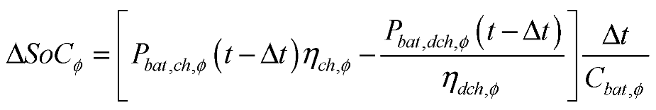 where is the total capacity of the battery; and are charging and discharging power of the battery, respectively; and are charging and discharging efficiency, respectively; Δt is the time segment (for example 1 h), and ϕ denotes the phase, ϕ(a,b,c).
Battery power and SoC must always be within defined limits, as follows:
where and are maximum charging and discharging powers of the battery, respectively; and are the predefined minimum and maximum charge levels, respectively; T is a time horizon, e.g. 24 h.
Battery charge/discharge power () and SoC are mutually dependent variables. Taking into account the variability of the electricity price, their relationship can be expressed as follows [12]:
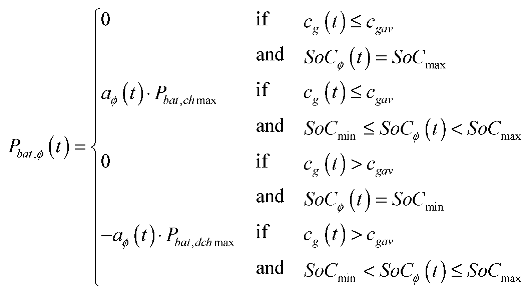 where is the day-ahead electricity price from the source grid at time t, is the average electricity price during the day; aϕ(t) is a coefficient within the range [0, 1].
The coefficient aϕ(t), which defines the power of the BESS, can be determined in different ways. In [12], the coefficient aϕ(t) is calculated based on the relation of the electricity price at the time t and the mean electricity price during a day. A similar approach was adopted in [16], where the coefficient aϕ(t) is calculated as a function of the difference in the electricity price from the predefined lower price limit for discharging and upper price limit for charging. However, the charging/discharging powers of the BESS determined in this way do not guarantee the optimal dispatch of the active power according to the adopted objective function. Therefore, in this paper, the coefficient aϕ(t) is considered as a control variable, whose value optimizes to ensure the minimization of a given objective function.
The basic equation of the active power dispatch problem is the power balance constraint (9), which must be satisfied at each time segment t:
where Pg,ϕ(t) is the active power from/to the source grid at time t in phase ϕ; PL,ϕ(t) is the total active power of the load at time t in phase ϕ; PPV,ϕ(t) is the total active power generation of PV units at time t in phase ϕ; Pbat,ϕ(t) is the active power of the battery at time t in phase ϕ; ϕ(a,b,c).
2.1. Objective Function for OAPD
By controlling the operating mode of the battery, i.e. the charging/discharging power and SoC, the active power flows in the distribution network can be significantly influenced. In this way, the exchange power with the source power grid is directly affected, as well as other parameters of the distribution networks, such as power losses, voltage profile, etc. The operating costs of the distribution network mostly depend on the value of the energy from/to the source grid. Considering various PV generation and load demand scenarios with their probabilities, the objective function for OAPD can be formulated as the minimization of the expected cost for electricity, as follows:
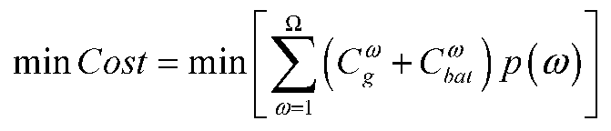
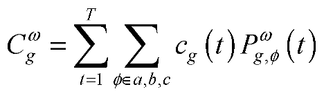
where ω and Ω are the current scenario and the total number of scenarios, respectively; p(ω) is the probability of scenario ω; and are the total cost for electricity from the source grid and operating cost of the battery in scenario ω, respectively; cg and are the electricity price from the source grid and the unit operating cost of the battery, and T is the considered period (i.e. 24 h).
Two assumptions should be kept in mind here, namely:
- The retail electricity prices have the same daily profile as the wholesale electricity prices and fluctuate hourly.
- The DN transacts with the wholesale markets through some energy agent such as an aggregator.
The power output of a PV source is determined by the solar irradiation at a given moment, and its value cannot be influenced. Therefore, the cost of the PV generation is not taken into account in the objective function (10), because it cannot be optimized with controlling the charge/discharge power of the battery.
For stable operation, constraints (3-7) and (9) must be satisfied. The output power of the PV generator is limited by the maximum output power, i.e. the nominal power. Also, Pg,ϕ(t) must be restricted by minimum and maximum values.
2.2. Modeling of Uncertainties
2.2.1. PV Generation Modeling
The power of the PV source as a function of solar irradiance can be expressed as follows [16]:
where Ppvn is the nominal power of the PV source; S is the solar irradiance on the PV module surface; Sstc is the solar irradiance under standard test conditions; Rc is a certain irradiance point.
To model the stochastic nature of the solar irradiance, it is most convenient to use the Beta probability density function (PDF):
where fb(S) is the Beta function of the solar irradiance S; α, β are the shape parameters of the Beta distribution; and Γ is the Gamma function.
Based on the data of the long-term measurement of the solar irradiance in a given area, characteristic daily diagrams of the solar radiation can be estimated, with statistical indicators, i.e. mean value (µS) and standard deviation of the solar irradiance (σS) in a given time interval t (e.g. an hour). Using mean value and standard deviation of the solar irradiance, the shape parameters of the Beta PDF can be calculated for a time interval t, as follows:
2.2.2. Load Modeling
The normal (Gaussian) probability function is most commonly used to model load uncertainty in distribution systems. Generally, the load level is assumed to be a random variable (L) following the same PDF within each hour of a given daily load diagram [2].
where μL and σL are the mean value and standard deviation of L, respectively; r is a random number in [0, 1]; and erf(·) and erf-1(·) are the error function and the inverse error function, respectively.
2.2.3. Scenario Generation
The Monte Carlo simulation (MCS) method is suitable to modeling the uncertainties of solar irradiance and load level. Starting from probability density functions for solar irradiance and load, whose parameters are determined based on historical data, eg previous years, the MSC method can generate a large number of scenarios for day-ahead profiles of solar irradiance and load levels. Although a larger number of scenarios (e.g. several thousand) provides a more faithful modeling of the uncertainty of the output power of the PV source and the load level, on the other hand, it means a higher computation burden. In distribution network operation control applications, such as optimal power flow, methods with high accuracy and low computational burden are needed.
As a compromise between a good approximation (modeling) of the uncertainty of stochastic input variables (solar irradiance and load) on the one hand, and a significant reduction in calculation time on the other hand, a scenario reduction strategy aggregating similar scenarios can be applied. In doing so, it must be ensured that the metric of probability distribution of the reduced set must be close enough to the original set of scenarios. There are several algorithms for reducing the number of scenarios, such as k-means clustering, backward reduction, and fast forward selection. In this work, the simultaneous backward reduction algorithm [17,18,19] was employed to reduce a ternary scenario tree for the daily PV generations and load profiles.
3. Optimal Reactive Power Dispatch
In this paper, it is assumed that PV arrays and batteries are connected to unbalanced DNs via single-phase converters. Depending on the nominal apparent power of the converter and the active power level of the corresponding PV source or battery, they have the ability to control the generation/absorption of reactive power, that is, they can be used as an additional regulation resource in DNs [12,20], as illustrated in Figure 1.
Therefore, for DNs with PV units and BESS, the problem of ORPD can be posed as a problem of determining the optimal reference values of the available reactive powers of the inverters and the slack bus voltage magnitudes with certain objective function, under specified active power outputs of all PV and BESS inverters representing the solution of the active power dispatch as explained in Section 2.
3.1. Objective Function for ORPD
3.1.1. Active Power Loss Minimization
The level of active power losses is one of the most important indicators of the efficiency of the distribution network management, because they represent the direct costs for a distribution company. Therefore, the minimization of active power losses is one of the most common and important objective functions in OPF studies used by distribution system operators. Considering different (reduced) scenarios for PV generation and load profiles with their respective probabilities, the objective function for ORPD can be formulated as a minimization of the expected daily energy loss, as follows:
where is the total energy loss in scenario ω; NB is the number of branches in the DN; is the resistance of the branch i in phase ϕ; is the current magnitude through the ith branch in phase ϕ for scenario ω.
3.1.2. Voltage Unbalance Minimization
High penetration of single-phase PV systems and relative variations in per-phase loading lead to an increase in voltage imbalance in distribution networks. It is well known that significant voltage unbalance may lead to higher network losses, increased heating of network components such as transformers, as well as costly damage or derating of three-phase motors [21]. In this paper, the phase voltage unbalance rate (PVUR) is used for the voltage unbalance metric. The PVUR is calculated at each three-phase bus using the line-to-ground voltage magnitudes Va, Vb, Vc [21]:
According to the IEEE standard 141-1993, the maximum value of PVUR must not exceed 2% for distribution networks. To ensure that the PVUR value at any three-phase bus does not exceed this limit, the minimization of the expected maximum of PVUR in the DN can be defined as an objective function:
where is the maximum value of the PVUR in the DN for scenario ω.
3.2. Constraints
3.2.1. Equality Constraints
3.2.2. Inequality Constraints
There are two types of inequality constraints: functional operational constraints such as slack bus active power limits (23), load bus voltage limits (24), and branch flow limits (25); and feasibility region constraints defined by inverter reactive power limits (26), and slack bus voltage limits (27).
where , and are the active power from/to the source grid at time t in phase ϕ, minimum and maximum power from/to the source grid, respectively; , , are the voltage magnitude at the load bus i in phase ϕ, minimum and maximum limits of the voltage magnitude at load buses, respectively; and are the apparent power value and maximum apparent power value of the ith branch in phase ϕ, respectively; is the reactive power injection of the inverter connected to phase ϕ at the ith bus, and are the maximum (rated) apparent power and the active power at time t of the PV (or BESS) inverter connected to phase ϕ at the ith bus, respectively; , and are the voltage magnitude value, minimum and mаximum limits of the voltage magnitude at the slack bus in phase ϕ, respectively.
4. Solution Method
The hybrid PSOS-CGSA algorithm introduced in [23] was applied to effectively solve the above defined optimal active/reactive power dispatch. This is a metaheuristic population-based optimization algorithm constructed by the hybridization of particle swarm optimization with sigmoid-based acceleration coefficients (PSOS) [24] and chaotic gravitational search algorithm (CGSA) [25]. Its performance in terms of simplicity, efficiency and robustness has been demonstrated in solving various complex optimization problems such as distribution system state estimation [23], dynamic economic dispatch [26], and optimal power flow in DNs [12].
4.1. Application of PSOS-CGSA for Active Power Dispatch
In the optimal active power dispatch problem presented in Section II, the objective function is defined by equation (10). The control variables are coefficients aϕ(t) which define the power of the BESS according to (8). Therefore, a search agent can be written as:
where N is the total number of search agents (population size), aϕ,i(t) is the value of control variable a within search agent i for phase ϕ at iteration t.
A summary of the proposed algorithm for solving the active power dispatch is represented by the flowchart in Figure 2.
4.2. Application of PSOS-CGSA for Reactive Power Dispatch
The vector of control variables in the problem of ORPD consists of the reactive powers of the PV and BESS inverters and the slack bus voltage magnitudes, and can be expressed as follows:
where is the reactive power of the inverter at the jth bus in phase ϕ, Ni is the total number of buses in which inverters are connected, is the voltage magnitude at the root bus of phase ϕ(a,b,c).
The application of PSOS-CGSA in solving the problem of optimal reactive power dispatch is presented with the flowchart in Figure 3.
5. Simulation Results
The proposed approach for the day-ahead optimal dispatching of active and reactive powers was simulated on a modified IEEE 13-bus feeder [27]. In the modified IEEE 13-bus feeder, the single-phase PV sources are connected to buses 634, 645, 646, 611, 675, 692 and 652, as shown in Figure 4. Single-phase PV sources, each with the same rated power of 250 kW, are connected to the grid via single-phase inverters. Single-phase BESSs, each with a rated power of 0.9 MW and a capacity of 3.6 MWh are connected at bus 680 in all three phases via single-phase converters rated apparent power 1.1 of the rated power of the batteries. Data on PV and BESS parameters are given in Table 1 and Table 2, respectively.
The daily load profile is assumed to be with the hourly mean values tabulated in Table 3 with the same standard deviation of 10% of the corresponding mean values. The simulation was performed for the daily solar irradiance profile with the hourly mean value and standard deviation as given in Table 4. The day-ahead electricity price (EP) data are adopted as in Table 5. The maximum value is estimated according to the electricity price for Serbia on the spot market in January-February, 2023.
5.1. OAPD Results
As explained in Section 2, using MCS, there are 2000 solar irradiace and load scenarios generated, as shown in Figure 5. By applying the simultaneous backward reduction technique, these 2000 scenarios were reduced to 10 scenarios shown in Figure 6.
By applying the proposed approach for the optimal active power dispatch, the expected total operating costs of each scenario were determined, and the results are shown in Table 6.
The optimal value of the expected daily cost for electricity is 453.16 (€). Acording to (10), this value is obtained as sum of the costs in each reduced scenario multiplied by the corresponding probability. In view of this, the expected day-ahead charging/discharging schedule of the BESS was obtained as shown in Figure 7 and Figure 8.
To fair comparison, Figure 9 shows the daily costs for electricity in the following cases: (i) without the BESS integrated into the DN - base case, (ii) with the BESS in the DN applying the charge/discharge schedule approach presented in [12], and (iii) with the BESS in the DN using the proposed OAPD algorithm. The results in Figure 9 clearly indicate that the proposed PSOS-CGSA-based approach for OAPD leads to a large reduction in costs for electricity compared to the base case and the approach for OAPD in [12].
5.2. ORPD Results
Here, the optimal values of 21 control variables should be determined, as follows:
The simulation studies performed for the following two test cases:
Case 1: Minimization of the active power losses (Fobj1)
Case 2: Minimization of the phase voltage unbalance rate (Fobj2)
The voltages at the load buses must be within [0.94 -1.06] (p.u.). The voltage of the root bus (V0) can be changed in the range [0.9 -1.1] (p.u.), while the limits of the reactive power of the converter are variable, according to (26).
The results are given in Table 7 and Table 8. In the base case, the PV sources and BESS operate with unity power factor, and the root bus voltage is equal to 1 p.u. Table 7 and Table 8, respectively, show the expected values of total active energy losses (Wloss) and maximum values of phase voltage unbalance rate (PVURmax) for all ten reduced scenarios.
Applying the proposed procedure for ORPD achieves a reduction of expected energy losses by 22% compared to the base case, while the expected value of the maximum PVUR drops from 9.1% to 1.91%. There are significant energy savings, and it is ensured that the PVUR index level is below the maximum limit of 2% for all three-phase buses in the DN.
Based on the results shown in Table 7 and Table 8, it can be seen that in the case of the minimization of active energy losses (Fobj1) the best scenario is 9, and in the case of the minimization of the voltage unbalance (Fobj2) the best scenario is scenario 1. Figure 10 and Figure 11 show the optimal values of the control variables for these best scenarios.
The voltage profiles at the bus 671 for the best scenario in Case 1 and the best scenario in Case 2 are shown in Figure 12 and Figure 13, respectively.
In Case 1, ORPD reduces the active energy losses compared to the base case, while the voltages are within the permissible limits, as shown in Figure 12. The phase voltage magnitudes are much closer to each other in Case 2 (Figure 13) than in Case 1 (Figure 12). Clearly, this is as a consequence of the PVUR minimization in Case 2.
5.3. Evaluation of PSOS-CGSA
Тhe efficiency of the proposed solution algorithm (PSOS-CGSA) was confirmed by a comparison with well-established metaheuristic algorithms PSO, GSA and theirs recent improved versions PSOS [24] and CGSA [25]. Algorithm parameters displayed in Table IX, are adopted based on their default values in the cited references. The population size and maximum iteration number are set as: N=50 and itmax=200 for all case studies. All algorithms were employed to solve the problem of OAPD under the same terms and input data.
The daily costs for electricity obtained for all 10 reduced scenarios are shown in Figure 14. It is clear that the proposed hybrid PSOS-CGSA method finds better solutions for the OAPD problem, i.e., provides lower costs in each of 10 scenarios compared to PSO, GSA, PSOS and CGSA algorithms.

Table 9.
Algorithms parameters.
| PSO | C1=2; C2=2; wmax=0.9; wmin=0.4 |
| GSA | G0=1; α=20; p=2; K0=1 |
| PSOS | C1i=0.5; C1f=2.5; λ=0.0001; wmax=0.9; wmin=0.4 |
| CGSA | G0=1; α=20; wmax=0.1; wmin=1e-10; Sinusoidal map |
| PSOS-CGSA | C1i=0.5; C1f=2.5; λ=0.0001; G0=1; α=20; Sinusoidal map |
6. Conclusion
In this paper, a two-stage approach for the dynamic day-ahead optimal active-reactive power dispatch in unbalanced DNs with high penetration of single-phase solar PV systems and BESS has been proposed. The simulation results conducted on a modified IEEE 13-bus test system indicate the conclusions that can be summarized as follows:
- The proposed OAPD ensures minimum costs for the electricity from the source grid for all scenarios generated by the MSC method and the simultaneous backward reduction algorithm.
- It has been shown that single-phase PV inverters and BESS can serve as additional reactive power management resources.
- The proposed ORPD approach enables the reduction of active power losses in the DN and reduction of the voltage unbalance on the three-phase load buses below the permitted limit.
- The proposed PSOS-CGSA solution technique provides better solutions for the optimal power dispatch problems compared to other well-established metaheuristic algorithms such as PSO, GSA, and modified PSOS and CGSA.
Author Contributions
Jordan Radosavljević: conceptualization, methodology, writing—original draft preparation; Aphrodite Ktena: writing—review and supervision; Milena Gajić, Miloš Milovanović and Jovana Živić: investigation, software, validation, visualization. All authors have read and agreed to the published version of the manuscript.
Funding
This research was funded by the Government of the Republic of Serbia, grant number TR 33046.
Conflicts of Interest
The authors declare no conflict of interest.
References
- IRENA, Renewable Power Generation Costs in 2020, International Renewable Energy Agency, Abu Dhabi, 2021.
- Radosavljević, J.; Arsić, N.; Milovanović, M.; Ktena, A. Optimal placement and sizing of renewable distributed generation using hybrid metaheuristic algorithm. Journal of Modern Power Systems and Clean Energy. 2020, 8, 499–510. [Google Scholar] [CrossRef]
- Luo, X.; Wang, J.; Donner, M.; Clarke, J. Overview of current development in electrical energy storage technologies and application potential in power system operation. Applied Energy. 2015, 137, 511–536. [Google Scholar] [CrossRef]
- Gabash, A. Active-reactive optimal power flow in distribution networks with embedded generation and battery storage. IEEE Transactions on Power Systems. 2012, 27, 2026–2035. [Google Scholar] [CrossRef]
- Mehrjerdi, H.; Hemmati, R. Modeling and optimal scheduling of battery energy storage systems in electric power distribution networks. Journal of Cleaner Production. 2019, 234, 810–821. [Google Scholar] [CrossRef]
- Adewuyi, O.B.; Shigenobu, R.; Ooya, K.; Senjyu, T. Static voltage stability improvement with battery energy storage considering optimal control of active and reactive power injection. Electric Power System Research. 2019, 172, 303–312. [Google Scholar] [CrossRef]
- Li, X.; Ma, R.; Gan, W.; Yan, S. Optimal dispatch for battery energy storage station in distribution network considering voltage distribution improvement and peak load shifting. Journal of Modern Power Systems and Clean Energy. 2022, 10, 131–139. [Google Scholar] [CrossRef]
- Milošević, D.; Đurišić, Ž. Technique for stability enhancement of microgrids during unsymmetrical disturbances using nattery connected by single-phase converters. IET Renewable Power Generation. 2020, 14, 1529–1540. [Google Scholar] [CrossRef]
- Watson, J.D.; Watson, N.R.; Lestas, I. Optimized dispatch of energy storage systems in unbalanced distribution networks. IEEE Transactions on Sustainable Energy. 2018, 9, 639–650. [Google Scholar] [CrossRef]
- Das, K.; Grapperon, A.L.T.P.; Sorensen, P.E.; Hansen, A.D. Optimal battery operation for revenue maximization of wind-storage hybrid power plant. Electric Power System Research. 2020, 188, 106–631. [Google Scholar] [CrossRef]
- Prudhviraj, D.; Kiran, P.B. S.; Pindoriya, N.M. Stochastic energy management of microgrid with nodal price. Journal of Modern Power Systems and Clean Energy. 2020, 8, 102–110. [Google Scholar] [CrossRef]
- Radosavljević, J.; Milovanović, M.; Arsić, N.; Jovanović, A.; Perović, B.; Vukašinović, J. Optimal power dispatch in distribution networks with PV generation and battery storage. In Proceedings of the IX International Conference on Electrical, Electronic and Computing Engineering IcETRAN 2022, Novi Pazar, Serbia, 6-9 June 2022.
- Giuntoli, M.; Subasic, M.; Schmitt, S. Control of distribution grids with storage using nested Benders’ decomposition. Electric Power Systems Research 2021, 190, 106663. [Google Scholar] [CrossRef]
- Khan, H.A.; Zuhaib, M.; Rihan, M. Voltage fluctuation mitigation with coordinated OLTC and energy storage control in high PV penetrating distribution network. Electric Power System Research. 2022, 208, 107924. [Google Scholar] [CrossRef]
- Radosavljević, J. Voltage regulation in LV distribution networks with PV generation and battery storage. Journal of Electrical Engineering. 2021, 72, 356–365. [Google Scholar] [CrossRef]
- Biswas, P.P.; Suganthan, P.N.; Amaratunga, G.A.J. Optimal power flow solutions incorporating stochastic wind and solar power. Energy Convers. Manage. 2017, 148, 1194–1207. [Google Scholar] [CrossRef]
- Gröwe-Kuska, N.; Heitsch, H.; Römisch, W. Scenario reduction and scenario tree construction for power management problems. In Proceedings of the 2003 IEEE Bologna PowerTech - Conference Proceedings, 2003, 3, 152–158.
- LNesp, scenred (https://github.com/supsi-dacd-isaac/scenred), GitHub. Retrieved February 22, 2023.
- Maheshwari, A.; Sood, Y.R.; Jaiswal, S. Flow direction algorithm-based optimal power flow analisys in the presence of stochastic renewable energy sources. Electric Power Systems Research. 2023, 216, 109087. [Google Scholar] [CrossRef]
- Ali, A.; Mahmoud, K.; Raisz, D.; Lehtonen, M. Probabilistic approach for hosting high PV penetration in distribution systems via optial oversized inverter with watt-var functions. IEEE Systems Journal, 2021, 15, 684–693. [Google Scholar] [CrossRef]
- Girigoudar, K.; Roald, L.A. On the impact of different voltage unbalance metrics in distribution system optimization. Electric Power System Research. 2019, 189, 106656. [Google Scholar] [CrossRef]
- Khushalani, S.; Solanki, K.M.; Shulz, N.N. Development of three-phase unbalanced power flow using PV and PQ models for distributed generation and study of the impact of DG models. IEEE Transactions on Power Systems. 2007, 22, 1019–1025. [Google Scholar] [CrossRef]
- Ullah, Z.; Elkadeem, M.R.; Wang, S.; Radosavljević, J. A Novel PSOS-CGSA Method for State Estimation in Unbalanced DG-integrated Distribution Systems. IEEE Access. 2020, 8, 113219–113229. [Google Scholar] [CrossRef]
- Tian, D.; Zhao, X.; Shi, Z. Chaotic particle swarm optimization with sigmoid-based acceleration coefficients for numerical function optimization. Swarm and Evolutionary Computation. 2019, 51, 100573. [Google Scholar] [CrossRef]
- Mirjalili, S.; Gandomi, A.H. Chaotic gravitational constants for the gravitational search algorithm. Applied Soft Computing. 2017, 53, 407–419. [Google Scholar] [CrossRef]
- Radosavljević, J.; Arsić, N.; Štatkić, S. Dynamic Economic Dispatch Considering WT and PV Generation using Hybrid PSOS-CGSA Algorithm. In Proceedings of the 20th International Symposium INFOTEH-JAHORINA (INFOTEH), East Sarajevo, Bosnia and Herzegovina, vol. no, pp. 1–6, 17-19 March, 2021.
- https://cmte.ieee.org/pes-testfeeders/resources/.
Figure 1.
Inverter capability curve. (a) Diagram of two-quadrant regulating capacity of a PV model, (b) Diagram of four-quadrant regulating capacity of a BESS model.
Figure 1.
Inverter capability curve. (a) Diagram of two-quadrant regulating capacity of a PV model, (b) Diagram of four-quadrant regulating capacity of a BESS model.

Figure 2.
Flowchart for the active power dispatch using PSOS-CGSA.
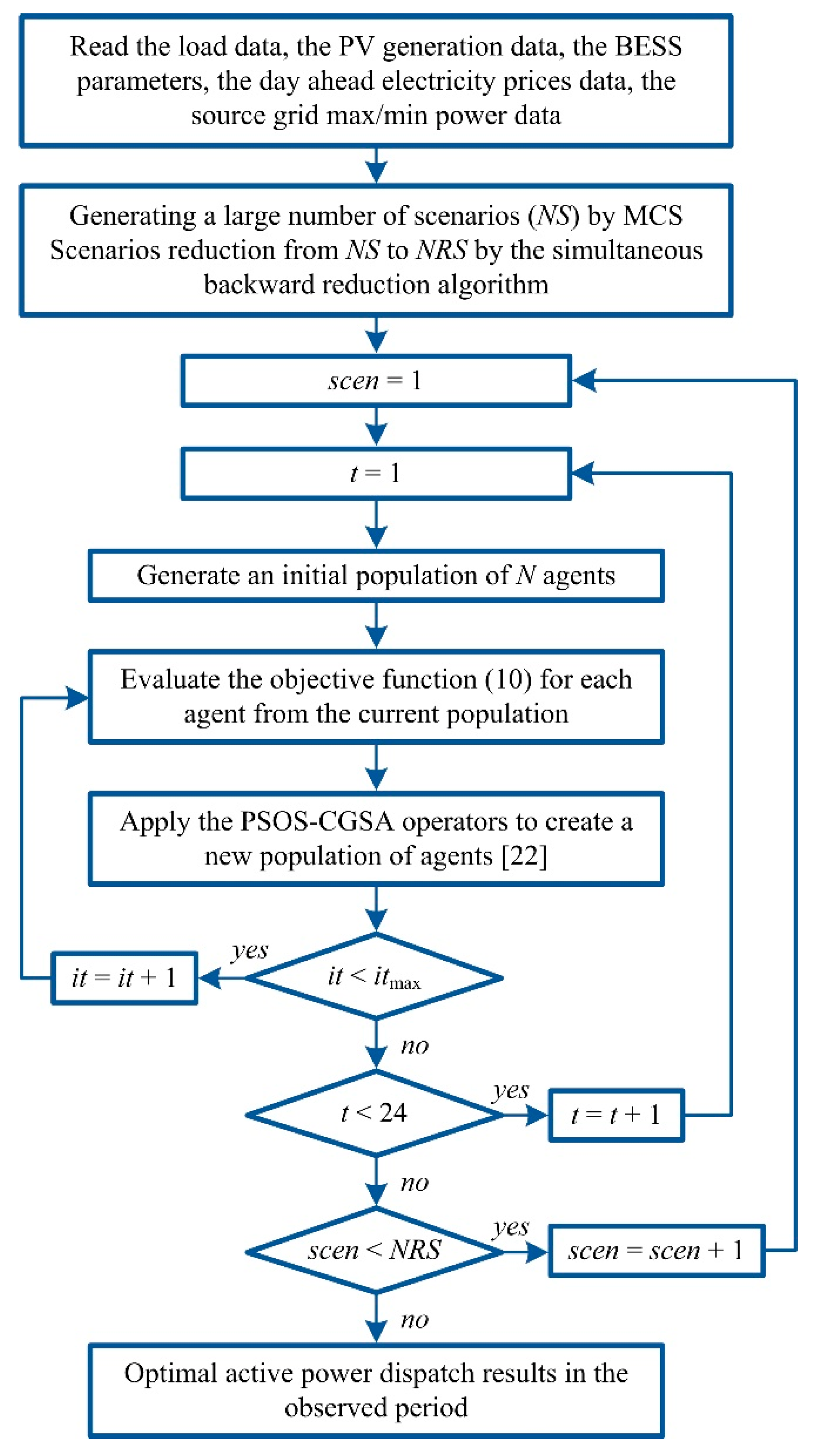
Figure 3.
Flowchart for the reactive power dispatch using PSOS-CGSA.
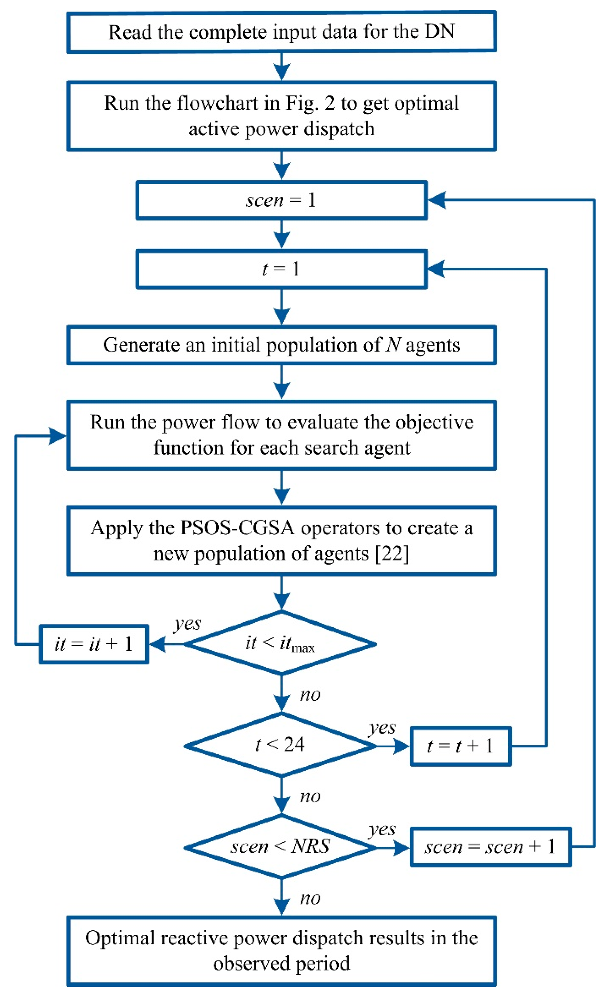
Figure 4.
Single-line diagram of the modified IEEE 13-bus test system.
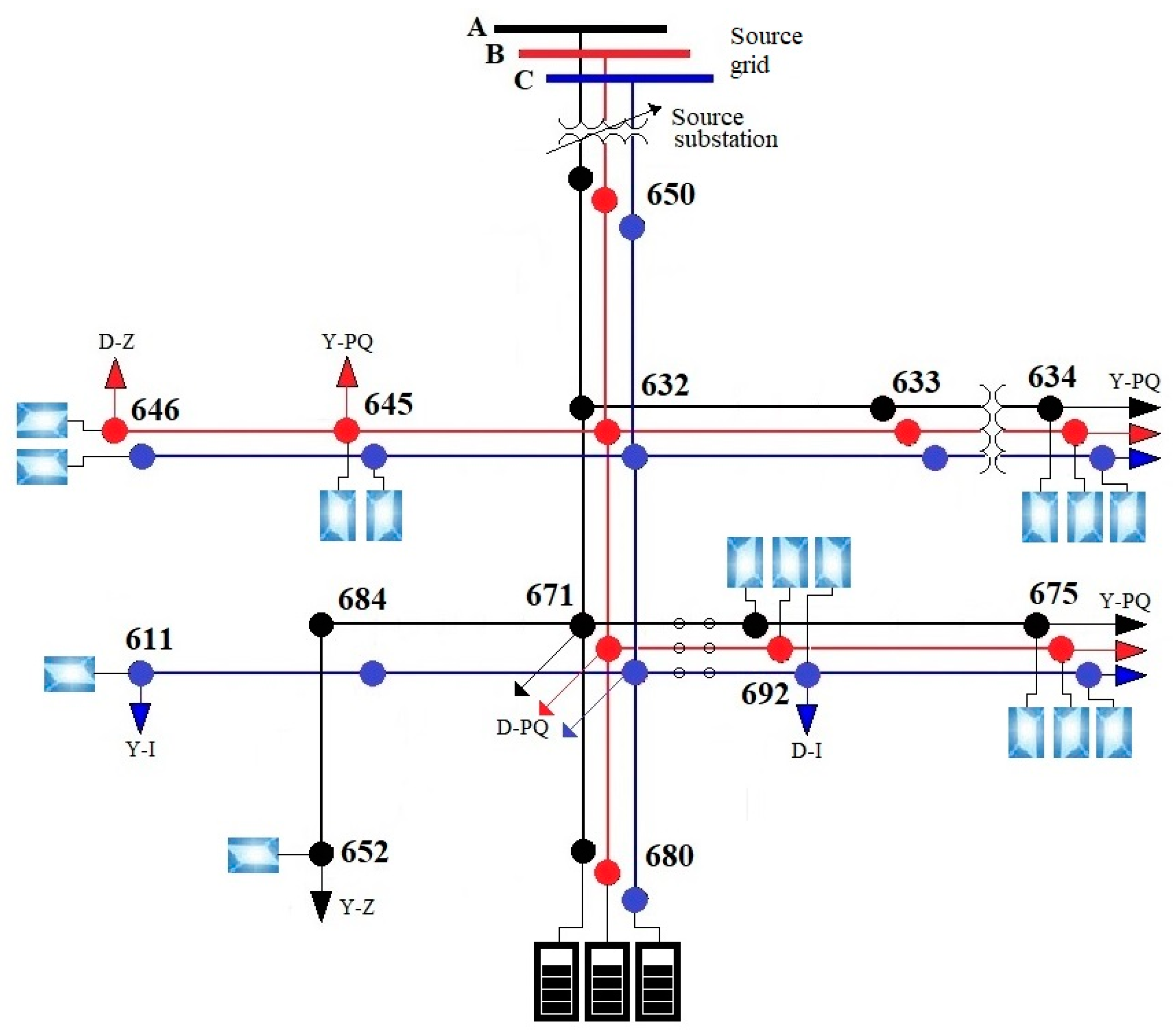
Figure 5.
Scenarios generated by MCS.
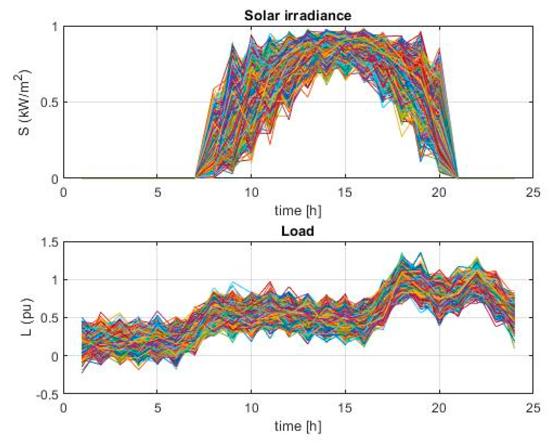
Figure 6.
Reduced scenarios of solar irradiance and load.
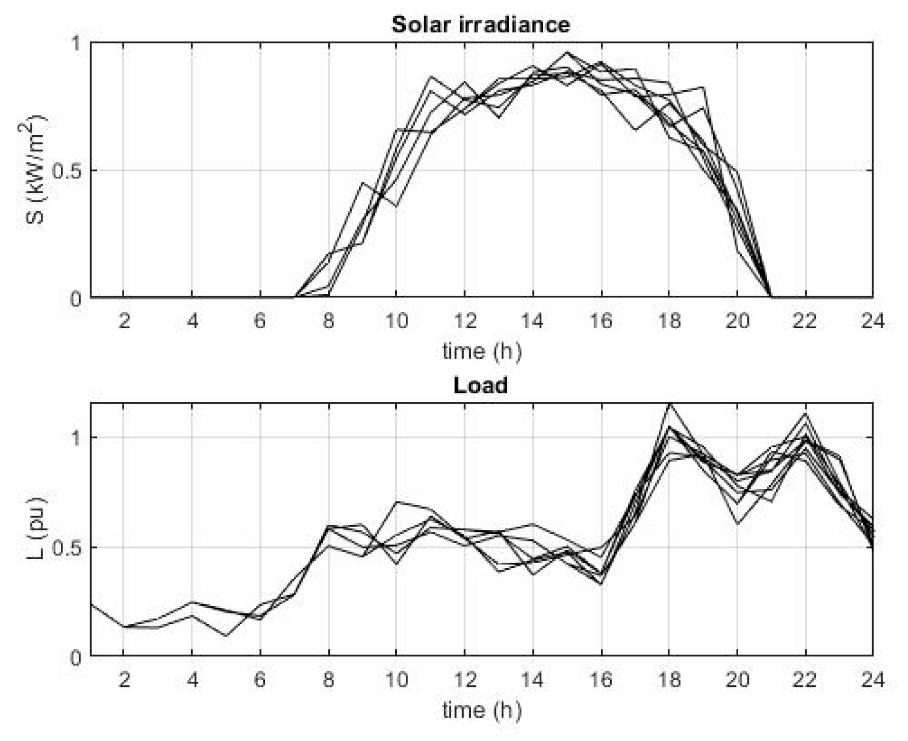
Figure 7.
Expected battery power during the day.
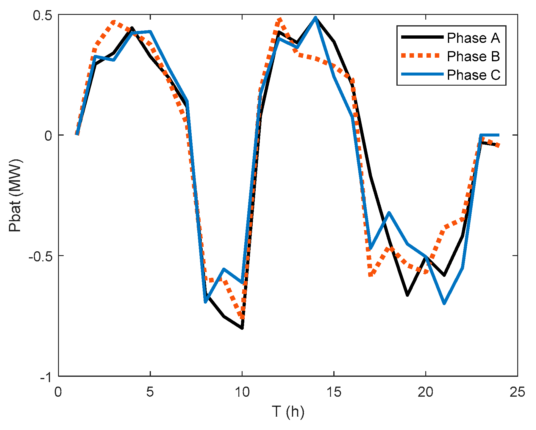
Figure 8.
Expected battery SoC during the day.
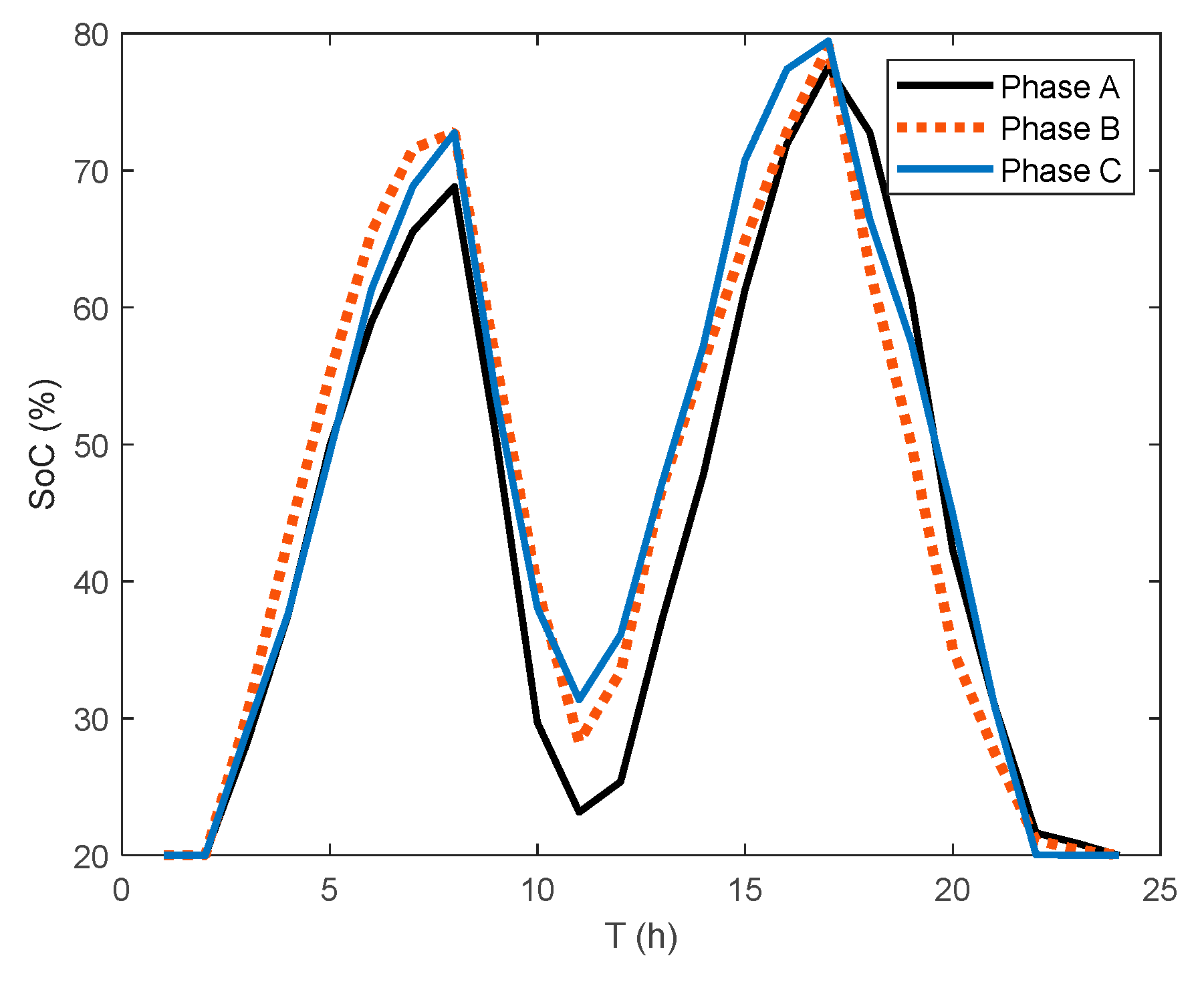
Figure 9.
Comparison of expected daily costs for electricity: (i) without BESS, (ii) with the BESS using approach in [12], (iii) with the BESS using the proposed OAPD algorithm.
Figure 9.
Comparison of expected daily costs for electricity: (i) without BESS, (ii) with the BESS using approach in [12], (iii) with the BESS using the proposed OAPD algorithm.
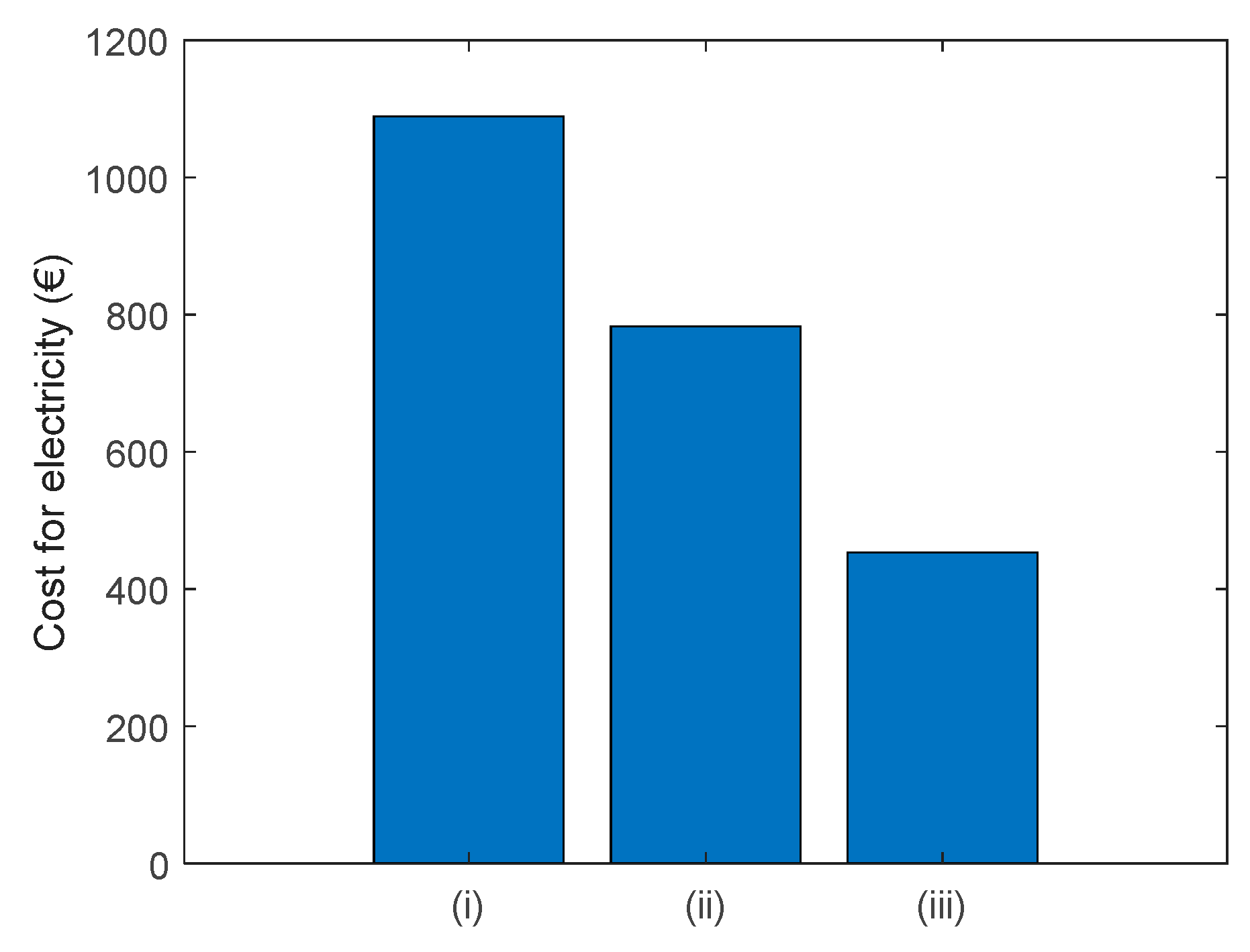
Figure 10.
Optimal values of control variables for the best scenario (9) in Case 1.
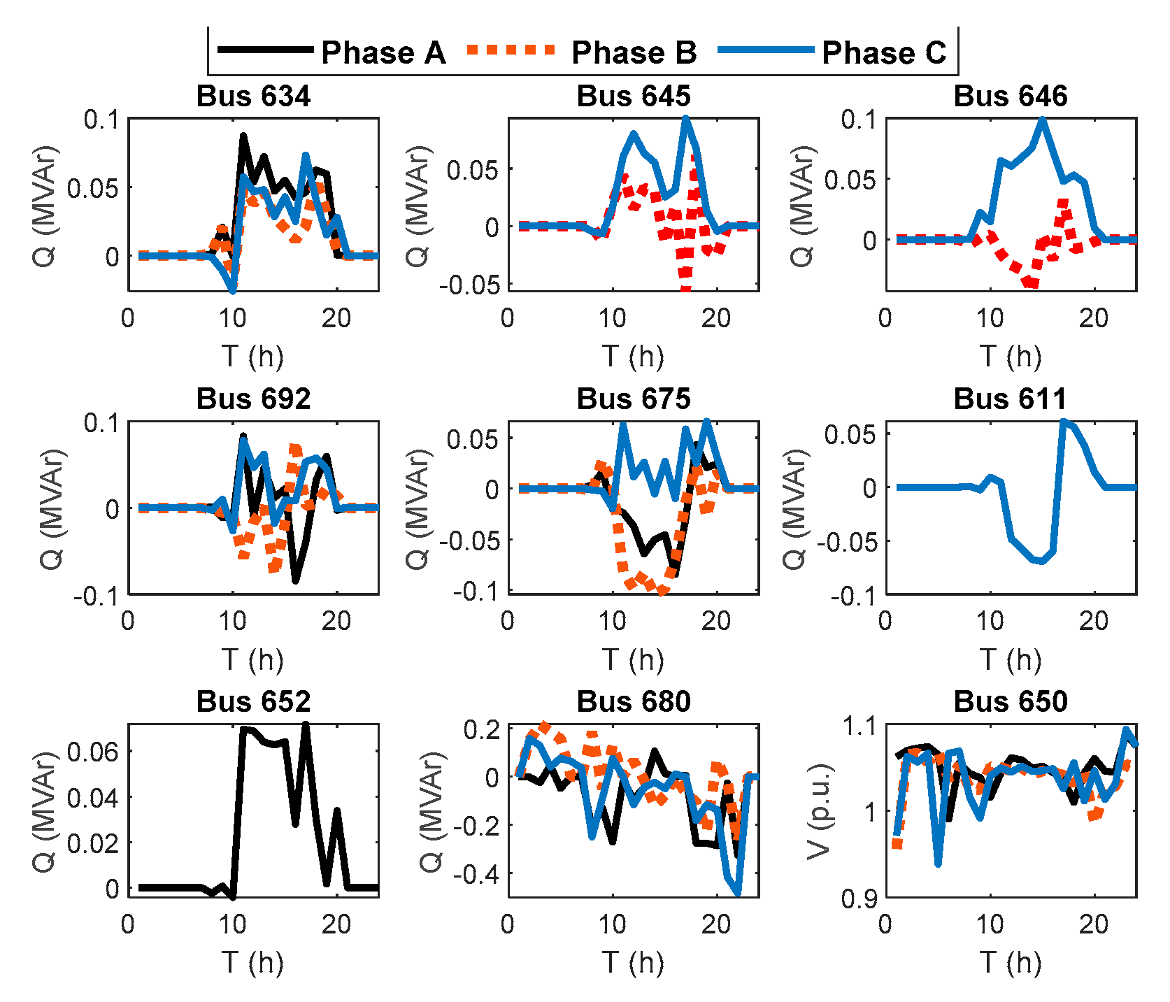
Figure 11.
Optimal values of control variables for the best scenario (1) in Case 2.
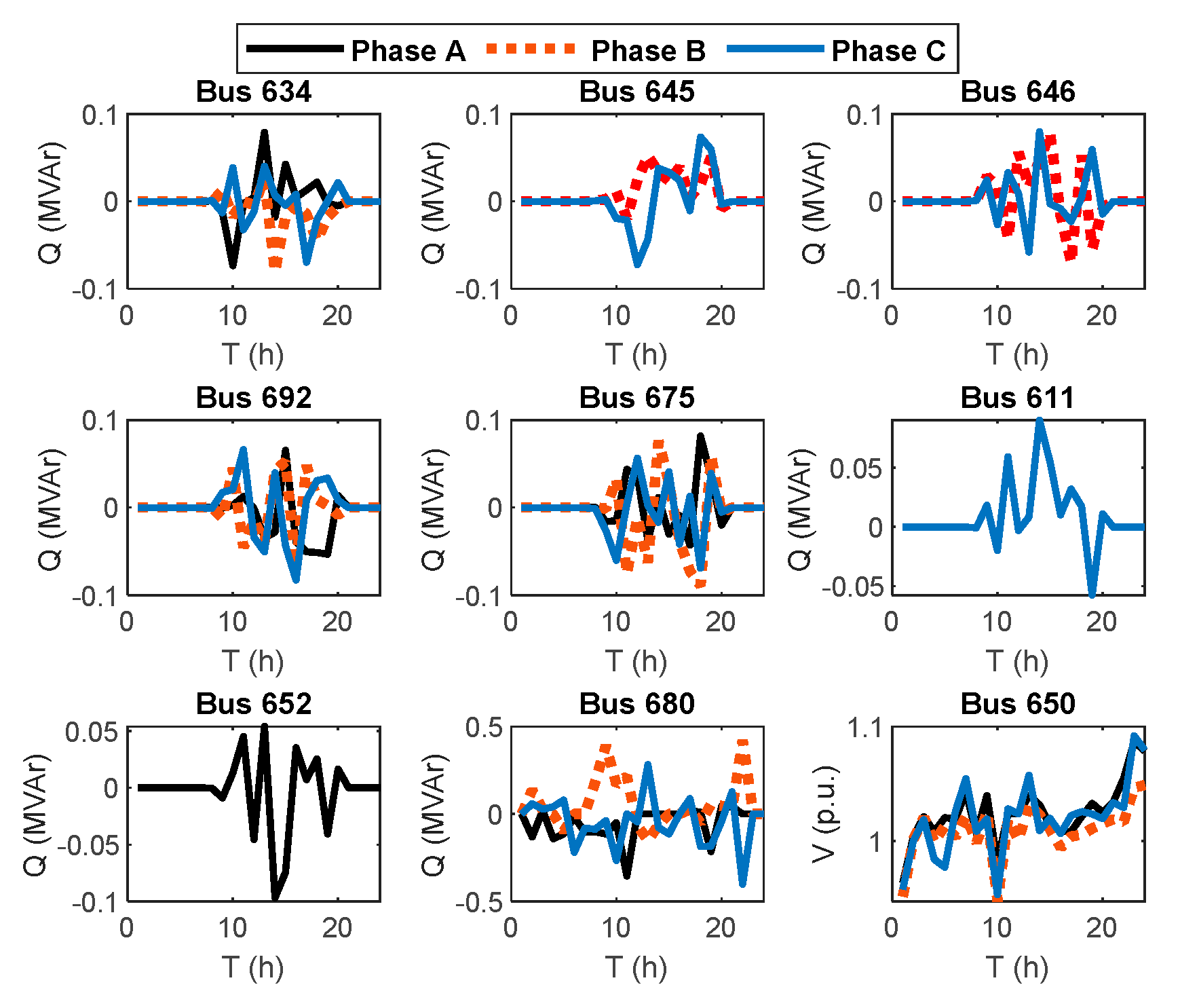
Figure 12.
Voltage profile at bus 671 in Case 1.
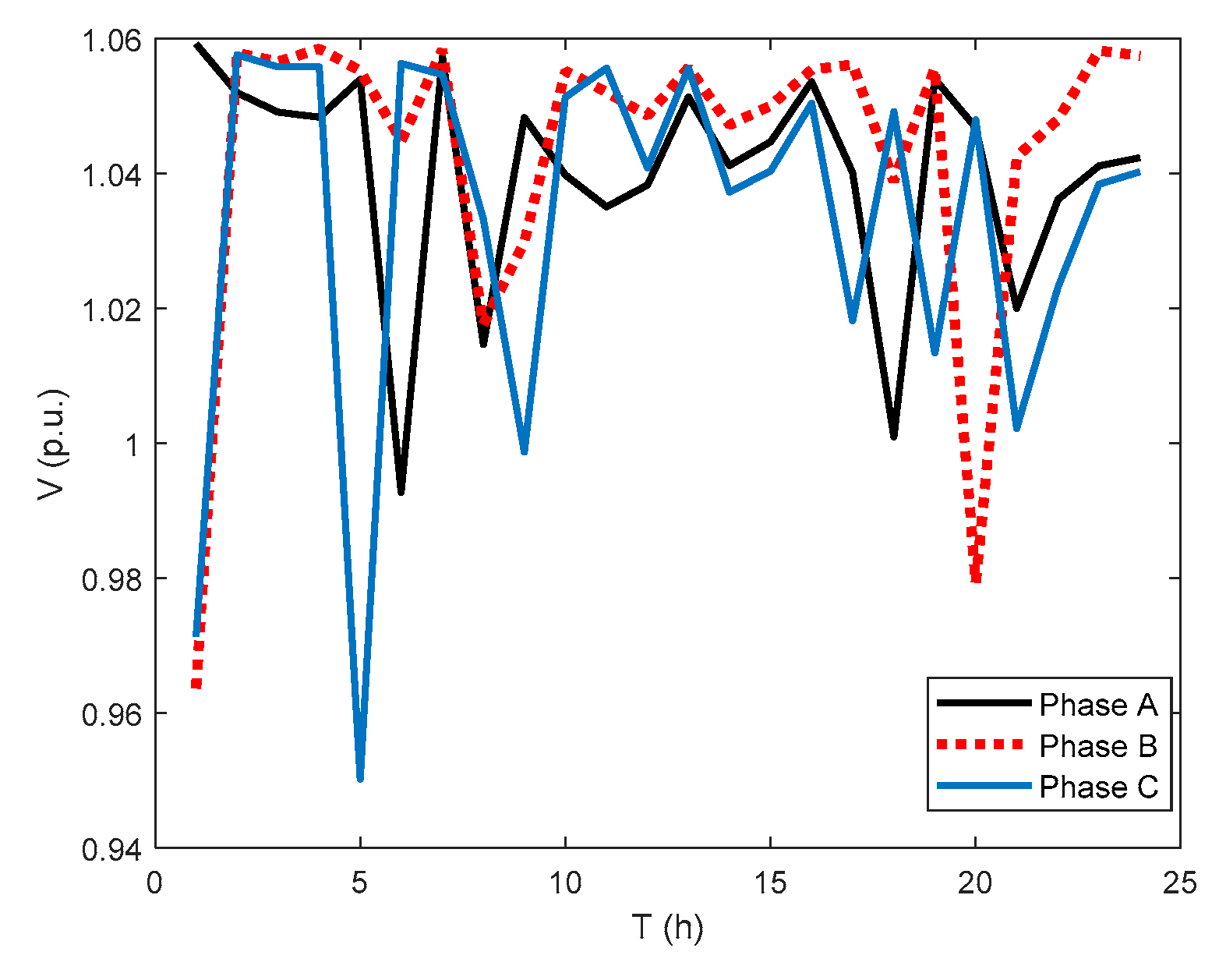
Figure 13.
Voltage profile at bus 671 in Case 2.
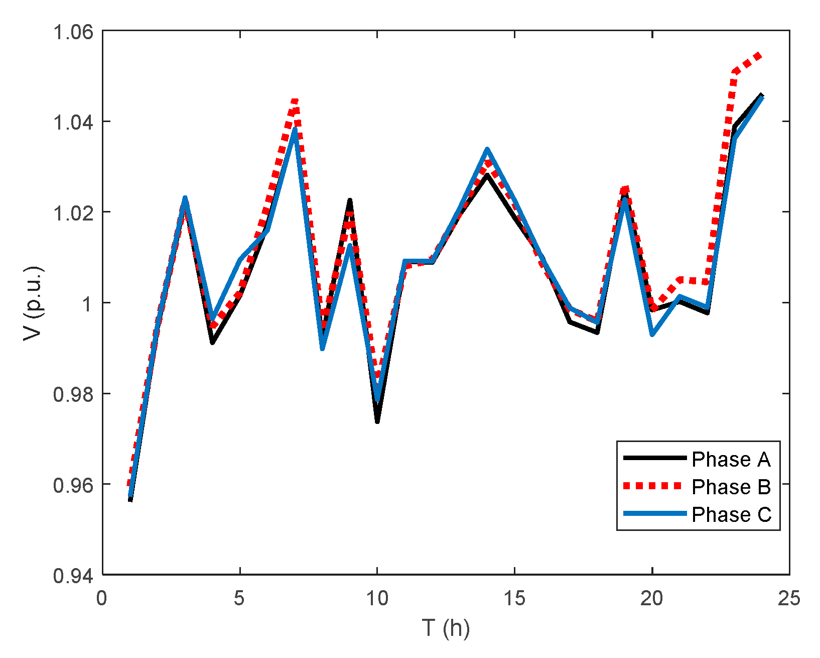
Figure 14.
Comparison of solution methods applied for OAPD.
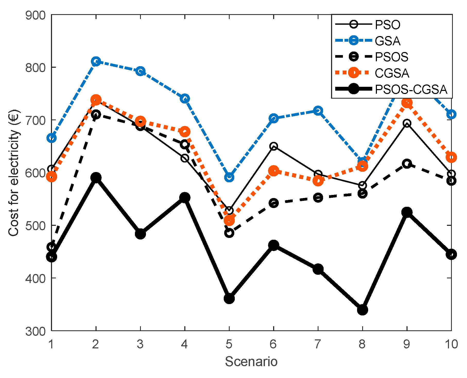
Table 1.
Parameters of PV units.
| Ppvn (kW) | Sstc (kW/m2) | Rc (kW/m2) |
|---|---|---|
| 250 | 1 | 0.12 |
Table 2.
Parameters of BESS.
| Pbat,chmax (MW) | Pbat,dchmax (MW) | SoCmax (%) | SoCmin (%) | ηch= ηdch | cbat (€/MWh) |
|---|---|---|---|---|---|
| 0.9 | 0.9 | 80 | 20 | 1 | 10 |
Table 3.
Load profile data.
| Hour | μL (p.u.) | Hour | μL (p.u.) | Hour | μL (p.u.) |
|---|---|---|---|---|---|
| 1 | 0.1591 | 9 | 0.5644 | 17 | 0.6715 |
| 2 | 0.2045 | 10 | 0.5372 | 18 | 1.0000 |
| 3 | 0.1948 | 11 | 0.6026 | 19 | 0.9310 |
| 4 | 0.1858 | 12 | 0.5496 | 20 | 0.7588 |
| 5 | 0.1963 | 13 | 0.4893 | 21 | 0.8244 |
| 6 | 0.1866 | 14 | 0.4847 | 22 | 0.9924 |
| 7 | 0.3154 | 15 | 0.4493 | 23 | 0.7869 |
| 8 | 0.5499 | 16 | 0.4390 | 24 | 0.5222 |
Table 4.
Solar irradiance data.
| Hour | μS (W/m2) | σS (W/m2) |
|---|---|---|
| 8 | 158 | 120 |
| 9 | 386 | 248 |
| 10 | 538 | 277 |
| 11 | 669 | 261 |
| 12 | 748 | 242 |
| 13 | 819 | 221 |
| 14 | 862 | 207 |
| 15 | 870 | 197 |
| 16 | 853 | 205 |
| 17 | 779 | 237 |
| 18 | 700 | 258 |
| 19 | 572 | 263 |
| 20 | 357 | 206 |
Table 5.
Electricity price data.
| Hour | cg (€/MWh) | Hour | cg (€/MWh) | Hour | cg (€/MWh) |
|---|---|---|---|---|---|
| 1 | 67.59 | 9 | 83.53 | 17 | 82.02 |
| 2 | 65.31 | 10 | 81.26 | 18 | 82.77 |
| 3 | 52.40 | 11 | 72.14 | 19 | 85.05 |
| 4 | 45.56 | 12 | 68.35 | 20 | 88.85 |
| 5 | 50.12 | 13 | 65.31 | 21 | 101.00 |
| 6 | 59.23 | 14 | 65.00 | 22 | 91.13 |
| 7 | 71.38 | 15 | 68.04 | 23 | 80.50 |
| 8 | 82.02 | 16 | 72.90 | 24 | 73.66 |
Table 6.
Expected costs.
| Scenario | Probability | Cost (€) |
|---|---|---|
| 1 | 0.04 | 440.22 |
| 2 | 0.08 | 590.36 |
| 3 | 0.06 | 483.70 |
| 4 | 0.08 | 552.52 |
| 5 | 0.06 | 361.21 |
| 6 | 0.11 | 462.06 |
| 7 | 0.23 | 416.95 |
| 8 | 0.13 | 339.61 |
| 9 | 0.12 | 524.65 |
| 10 | 0.11 | 444.86 |
| Expected | 453.16 |
Bold indicate the best results.
Table 7.
ORPD results for Wloss.
| Scenario | Probability | Wloss (kWh) | ||
|---|---|---|---|---|
| Base | Case 1 | Case 2 | ||
| 1 | 0.04 | 969.62 | 725.76 | 849.90 |
| 2 | 0.08 | 931.60 | 730.77 | 859.22 |
| 3 | 0.06 | 878.93 | 681.53 | 813.92 |
| 4 | 0.08 | 931.63 | 726.75 | 879.11 |
| 5 | 0.06 | 973.22 | 761.71 | 882.67 |
| 6 | 0.11 | 1016.80 | 805.72 | 951.66 |
| 7 | 0.23 | 937.08 | 724.04 | 873.22 |
| 8 | 0.13 | 990.97 | 776.68 | 919.96 |
| 9 | 0.12 | 804.23 | 616.91 | 759.31 |
| 10 | 0.11 | 977.61 | 772.15 | 905.42 |
| Expected | 940.44 | 732.62 | 873.16 | |
Bold indicate the best results.
Table 8.
ORPD results for PVURmax.
| Scenario | Probability | PVURmax (%) | ||
|---|---|---|---|---|
| Base | Case 1 | Case 2 | ||
| 1 | 0.04 | 12.54 | 7.70 | 1.14 |
| 2 | 0.08 | 10.45 | 6.46 | 2.93 |
| 3 | 0.06 | 8.42 | 7.43 | 2.05 |
| 4 | 0.08 | 8.97 | 7.32 | 1.51 |
| 5 | 0.06 | 11.91 | 6.46 | 2.75 |
| 6 | 0.11 | 10.01 | 7.85 | 2.67 |
| 7 | 0.23 | 8.34 | 6.46 | 1.71 |
| 8 | 0.13 | 8.06 | 6.83 | 1.16 |
| 9 | 0.12 | 6.46 | 7.58 | 1.46 |
| 10 | 0.11 | 10.55 | 6.43 | 2.29 |
| Expected | 9.10 | 6.96 | 1.91 | |
Bold indicate the best results.
Disclaimer/Publisher’s Note: The statements, opinions and data contained in all publications are solely those of the individual author(s) and contributor(s) and not of MDPI and/or the editor(s). MDPI and/or the editor(s) disclaim responsibility for any injury to people or property resulting from any ideas, methods, instructions or products referred to in the content. |
© 2023 by the authors. Licensee MDPI, Basel, Switzerland. This article is an open access article distributed under the terms and conditions of the Creative Commons Attribution (CC BY) license (http://creativecommons.org/licenses/by/4.0/).
Copyright: This open access article is published under a Creative Commons CC BY 4.0 license, which permit the free download, distribution, and reuse, provided that the author and preprint are cited in any reuse.


