Submitted:
08 July 2025
Posted:
09 July 2025
You are already at the latest version
Preprints on COVID-19 and SARS-CoV-2
Abstract
ORF7b is a tiny accessory protein of the SARS-CoV-2 virus of only 43 amino acids that is often believed similar to its homolog ORF7b of SARS-CoV. This study compared physico-chemical and structural properties of the two proteins, where necessary, to emphasize differences and similarities. However, the aim is to evidence the real properties of ORF7b of SARS-CoV-2, a protein functionally involved in many metabolic compartments. Sequence analysis and electrostatic characteristics show a polypeptide with both ends negatively charged and a diffuse negative charge over the entire structure. Its behavior in solution is like that of a polyanion with a net charge of −4 at neutral pH. Two modeling systems with ab initio features, were used to have a complete 3D-structure. The two best 3D-models are similar, as confirmed by the Ramachandran plot, and show a helical core with two disordered and fluctuating ends. Residue-residue analysis and normal mode analysis characterized the hinges of the protein and movements of rigid parts, confirming fluctuating extremities, which have a role in controlling the structural organization. The dipole moment calculation reveals a vector misaligned with the structure’s main axis, tilting outward by 24°. Molecular dynamics show a behavior in water in agreement with the previous results and structural distortions with a low tendency to solvate in an apolar environment. The definition of its thermodynamic association ranges discovered the intriguing potentiality to participate in liquid-liquid phase transitions (droplets) together with other viral proteins. ORF7b also shows a high sensibility to pH changes, with a widespread distribution of its negative surfaces dynamically adjusted by structural changes. In particular conditions, it is also quite soluble in aqueous media. ORF7b2’s intriguing properties and the vast number of its interactions, as reported in BioGRID, show its remarkable tendency to bind many molecular partners using both electrostatic and hydrophobic interactions in different cellular environments. This introduces additional considerations for ORF7b2 as a peripheral membrane protein, because of its unique chemical, physical, and structural characteristics, as well as its involvement in various metabolic compartments.
Keywords:
ORF7b of SARS-CoV-2
; COVID-19
; 3D-structure
; molecular dynamics
; dipole vector
; electrostatic properties
; protein flexibility
; SARS protein interactions
; RIN analysis
; peripheral membrane protein
1. Introduction
ORF7b-like folds have a protein family membership “Non-structural proteins 7b, SARS-like” (IPR021532) (also known as accessory proteins 7b, NS7B, ORF7b, and 7b) from human coronaviruses [1,2]. Coronaviruses conserve this sequence, suggesting functional conservation, but it shows no significant homology to human or unrelated proteins [3,4]. The only significant similarity detected is a seven-amino acid sequence (IIFWFSL26-32) like a part of the human olfactory receptor 7D4151-157, suggesting a role in viral-induced smell loss. However, the conservation of ORF7b among coronaviruses suggests an important role in the virus’s biology [5]. No one has yet experimentally defined a well-established 3D model of the ORF7b fold, nor studied its chemical-physical characteristics. A search on RCSB PDB, including Computed Structure Models from AlphaFold DB and ModelArchive, yielded negative results. This means that there are still no reliable models that fully reflect the functional characteristics of these proteins. ORF7b is also an accessory protein for SARS-CoV-2 [UniProtKB Accession: P0DTD8-1]. It comprises 43 amino acid residues [1], one less than the orthologous SARS-CoV protein [Table 1]. Both proteins (described here as ORF7b1 and ORF7b2, from SARS-CoV and SARS-CoV-2), share 85.4% identity and 97.2% sequence similarity, but show a different composition of charged amino acids [2,6,7]. Researchers consider accessory proteins not essential for viral replication but involved in pathogenesis. However, major structural proteins, such as the spike protein, overshadow coronavirus accessory proteins, like ORF7b.
ORF7b2 interacts with very numerous proteins in the human proteome. Indeed, the BioGRID curated project on physical protein interactions between SARS-CoV-2 and the human proteome (BioGRID COVID-19 Coronavirus Curation Project (https://thebiogrid.org/search.php?search=SARS-CoV-2*&organism=2697049, accessed on June 20, 2025) collects for ORF7b2 1,765 unique interactors that interact experimentally in vivo through 2,986 raw interactions. However, a rough consideration tells us that ORF7b2 might interact with a smaller number of proteins in the human proteome. In fact, not all interactions have the same statistical significance because of the various extraction technologies used by the various laboratories in their cellular models. However, even if the actual interacting proteins were less than half, this would imply that the protein must have a mechanism to reach and interact with these proteins in multiple cellular compartments. An AP-MS analysis (Affinity-Purification-Mass-spectrometry) identified 332 high-confidence protein interactions between SARS-CoV-2 proteins and human proteins [41]. This article was one of the first to understand that each viral protein could interact with many human different proteins, on average eleven. But, to get an effective physical interaction in a crowded environment such as that of the cell, it is necessary that the interacting molecules have not only an optimal affinity and good quantitative ratios but also similar spatio-temporal characteristics, because they must meet in a certain place at a specific time. This is still a limitation of today’s research.
We recently studied the functional activities of ORF7b2 by interactomic techniques, using only significant and experimentally validated interactions [9]. The protein is functionally involved in 5,057 functional terms of 15 categories [9] with biological functions spread in many and different intracellular locations, both membrane and cytosol related. It is involved [9] in signaling, immunological processes, in the nervous system, in membrane trafficking, in hemostasis, in insulin signaling, on the cell surface, in platelet-related processes, in cell-cell communication, in viral m-RNA translation, in a vast number of human tissues, even very far from the main sites of infection, such as the central nervous system and the male and female reproductive system [9]. We also discovered multiple interactions between ORF7b2 and other viral and human proteins [10] (see Excel file S3 in Supplements of [10] check). The limited spatiotemporal information, however, prevents a precise description of the molecular mechanisms behind these multi-to-one attacks [11]. One of ORF7b2 peculiarities is that of interacting also in a one-to-one manner with 9 specific human proteins during SARS-CoV-2 liver infection [12] (see Excel file S3 in Supplements of [12] check). Each of these nine proteins (ERBB4, GRB2, ITGA7, KCNMB4, LPAR1, ORAI1, RPS4Y2, RSRC1, and VTI1A) shows specific cellular locations and functions. For example, LPAR1 is a G-coupled receptor, located both on the cell surface and in the cytoplasm, but also in the endosome, and RPS4Y2 is a ribosomal protein of the small cytosolic subunit. This highlights the protein’s ability to populate diverse cellular locations with varying chemical-physical properties and interact with structurally distinct proteins. We found ERBB4 and GRB2 among the liver proteins involved in hepatitis B and hepatocellular carcinoma by SARS-CoV-2 infection [13], from which we inferred ORF7b2 might be involved also in these pathological processes. However, these considerations require further investigation.
The biological success of the virus is based on its exceptional ability to neutralize the host organism’s defenses through its set of proteins. Many of them counteract cellular defensive responses, such as interferon production or immune suppression. The author of an atlas on SARS-CoV-2 proteins [14] suggested that 21 viral proteins concur in blocking the interferon immune response and among them inserts ORF7b2. Selective interaction of ORF7b2 with the mitochondrial antiviral signaling protein (MAVS) inhibits the RLR signaling pathway, providing a mechanism for suppressing innate immunity and facilitating infection and viral production [15]. Toft-Bertelsen et al. [16] identified ORF7b2 as a novel viroporin. This observation suggested that ORF7b2 could act as an ion channel.
In vitro studies on cell-model systems produced many functional hypotheses for ORF7b2, often by invoking a structural similarity with ORF7b1 [7,17,18]. A recent study localized ORF7b2 in the endoplasmic reticulum (ER) region [18]; while older studies located ORF7b1 check in the Golgi compartment [19,20,21] and identified a leucine zipper sequence within its trans-membrane segment [19]. On this basis, a report has hypothesized that ORF7b2 too is a transmembrane protein localized in the Golgi apparatus [22] where these two proteins should functionally operate. This suggested a behavioral similarity. However, ORF7b2’s extensive studies reveal a very broad multifunctional activity with many implications for the pathogenesis of infection across many metabolic compartments. Researchers have often compared ORF7b2 to ORF7b1 because of their homologous properties and functions. But, even if ORF7b1 is a protein localized in the Golgi, only indirect evidence links ORF7b2 to this environment. All this suggests we should not consider its activity as confined to Golgi or ER membranes, also considering that its structure must possess peculiar characteristics to allow it to physically interact in vivo with 1,765 different proteins of the human proteome.
The numerous functions of ORF7b2 underscore a multifaceted role in SARS-CoV-2 biology and the pathogenesis of infection. All these features highlighted the need to know the structural organization of this protein. The lack of its three-dimensional structure has led researchers to perform many simulations, often focusing only on the central helical segment. However, because we do not know the complete structural organization of ORF7b1 and ORF7b2, many important structural details are still missing. Focusing only on the central helical segment, while ignoring the structural and functional roles of the long terminal segments, is problematic. These details are important for understanding the correct behavior of this protein in the various environments where it must interact to express a function. It is common in research activities, when faced with a poorly understood protein system, to integrate one’s data with those from homologous proteins. This approach has often prompted to compare ORF7b2 to ORF7b1 [18,23,24,25] assuming similar localizations and similar cell environments to perform corresponding functions. This approach is guiding the study of these two proteins until today.
However, there have also been recent studies to model the protein structure. According to some authors, ab initio modeling (Robetta) identifies three distinct top-scoring monomer structures for ORF7b2: a) a structure with a central 9-29 helical segment and two mobile and disordered tails; b) a slightly bent central helix with two very flexible tails; c) a structure almost entirely helical and rigid [26]. These same authors also conducted multiscale molecular dynamics simulations to provide detailed molecular insights into the helix-helix association as homodimers in the POPC bilayer. Their simulations showed the two best homodimer models can have both parallel and antiparallel orientations, even if with some distortions. However, the authors conclude that the functional organization of ORF7b is unclear regarding its orientation (parallel vs. antiparallel).
Other authors have shown that reconstituted ORF7b2 generates a dimer-tetramer equilibrium, but a monomer–dimer–tetramer equilibrium in the presence of reducing agents [27]. This suggests that the protein may have a tendency to form disulfide bonds, even in vivo. Biophysical measurements, such as NMR, electrophoresis, ultracentrifugation, and infrared spectroscopy have been used to promote their models in media mimicking the membrane environment [27]. However, the article fails to take into account that the widespread use of deuterated water in the solutions under study compacts and distorts the protein structure. Forgeon et al. hypothesized that ORF7b2 might interfere with those cellular processes that involve a leucine-zipper, forming multimers [28,29]. These same authors [29] have also used the transmembrane helices of PLN (phospholamban) as a static reference model for the structure, showing that an arrangement of the leucine zipper is sterically possible. Because their local AlphaFold software calculated a model showing a distorted leucine-zipper motif, they hypothesized two different ORF7b2 multimeric models. They also showed that their hypotheses were possible in vitro by mimicking a lipid environment. However, the real problem is not so much defining rigid organizational parameters of the structure to find behavioral analogies with similar proteins, but understanding what overall chemical-physical characteristics the protein possesses that, reflecting on its structural organization, allow it to operate in such different environments.
Currently, the most accepted model is the helical one where the central segment (residues 9-29) should favor a trans-membrane insertion (see Figure1S). Therefore, scientists classify ORF7b2 as a trans-membrane protein of the Golgi apparatus, probably at the endoplasmic level. This localization is consistent with its functional role in the immune system and modulation of cellular response. Although ORF7b does not have sites for post-translational modifications (PTMs), nor does it show the signal peptide to enter the Golgi, this does not exclude its function in the Golgi apparatus. It may act as a modulator or regulator of other modified proteins, rather than as a protein that requires chemical modifications to perform its function.
However, ORF7b2 appears to be a traveling protein, not a sedentary protein. A different picture emerges when considering its numerous functions and subcellular locations. The discovery of ORF7b2 functions in different cellular substructures or fluids (Golgi, mitochondria, plasma membrane, seminal liquid) suggests that the protein must have a dynamic role, having to adapt to different cellular needs. This mobility allows the protein to interact with different cellular structures and to perform multiple functions in various contexts. Although existing data do not yet allow us to unravel its complex structure-function paradigms, it is precisely its apparent mobility and its different locations that push towards more detailed studies. Viral proteins interact with host cellular machinery; however, they frequently occupy multiple compartments [30]. Their ability to interact and influence various organelles is strategic for the virus to manipulate cellular processes in its favor. All of this implies that viral proteins must have mechanisms to reach and interact with these compartments, and ORF7b2 is a viral protein.
The structural properties of mini-proteins such as ORF7b2 and ORF7b1 are frequently elusive [31,32]. Thus, we should also consider the set of their physicochemical properties to explain their structural and functional behaviors. This is based on the principle that it is the structural fluctuation that mediates the structure/function paradigm [33,34,35]. The structural fluctuations of proteins are closely linked to their physicochemical properties through the movements of their atoms, side chains, and structural domains. Therefore, whatever the cellular location where an ORF7b-like fold performs its activity, it must possess all those specific physical-chemical characteristics that allow it to function. ORF7b2 should also be subject to this rule.
This study aims to understand the functions of ORF7b2 by analyzing its sequence, physicochemical and electrostatic properties, stability, residue interactions, low-frequency normal modes, and molecular dynamics, using a complete 3D-model and comparing it to ORF7b1 where applicable. ORF7b2 should possess all those physicochemical properties necessary to satisfy its multiple functional activities.
2. Materials and Methods
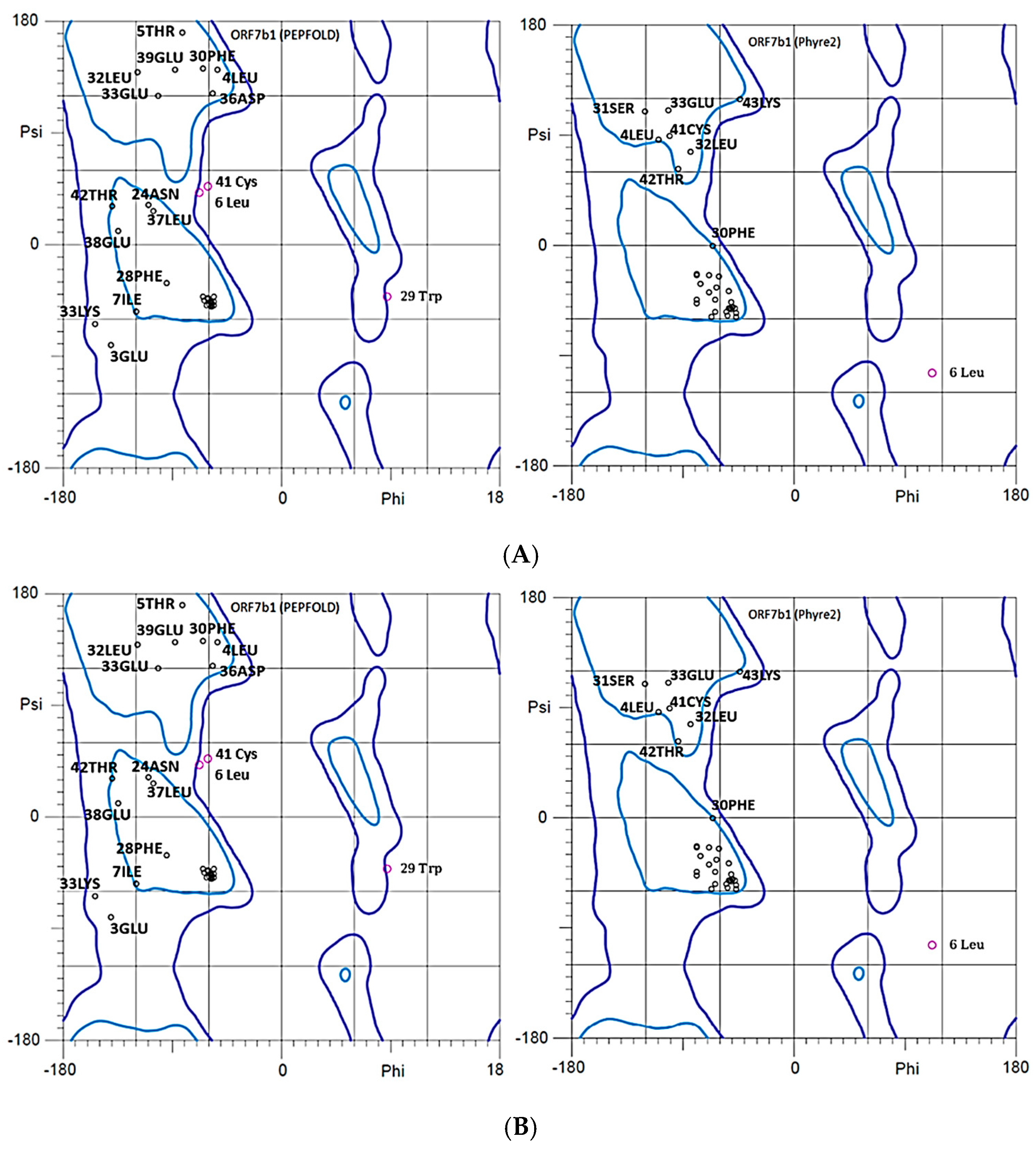
Electrostatic properties - The charge distribution of the proteins was evaluated in agreement with Das and Pappu [36,37,38,39]. Particularly, we calculated the fraction of charged residues, as FCR = |f+ + f−|, and the net charge per residue, as NCPR = |f+ - f−|. In this context, f+ and f− represent the fraction of positive and negative charges, respectively. These calculated values allow one to classify the protein sequences into distinct regions of the Diagram of States for IDPs: [38] (i) weak polyampholytes and polyelectrolytes named as Region 1 with values of FCR<0.25 and NCPR<0.25 and propensity for ensembles of Globule and Tadpole; (ii) a boundary region or Region 2 between 1 and 3 characterized by 0.25 ≤ FCR ≤ 0.35 and NCPR ≤ 0.35 values; (iii) strong polyampholytes (Region 3) with FCR > 0.35 and NCPR ≤ 0.35, and propensity for ensembles of Coils, Hairpins, and Chimeras; and (iv) strong polyelectrolytes (Region 4) where FCR > 0.35 and NCPR > 0.35, with a propensity for ensembles of Swollen Coils. Finally, we have calculated the parameter k to distinguish between different sequence variants based on the linear sequence distributions of oppositely charged residues [36,37,38]. We calculated the overall charge asymmetry as σ = (f+ - f−)2/(f+ + f−). For each sequence variant, we calculated k by partitioning the sequence into Nblob overlapping segments of size g. For each g residue segment, we calculated σί = (f+ - f−)2ί/(f+ + f−)ί , which is the charge asymmetry for the sequence of interest. We quantified the squared deviation from σ as:
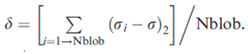
We used g = 5 and hypothesized different sequence variants, evaluating different values of δ for each. Hence, the maximal value δmax for an amino acid composition was used to define k = (δ/δmax).
Net Charge Calculation - The net charges of proteins at a given pH are based on the formula below:
Z = ∑i Ni [10pKai/(10pH + 10pKai)] - ∑j Nj [10pH/(10pH + 10pKaj)]
Where Z is the Net charge of the peptide sequence. Ni: Number of arginine, lysine, and histidine residues and the N-terminus; pKai, pKa values of the N-terminus and the arginine, lysine, and histidine residues; Nj, the Number of aspartic-acid, glutamic acid, cysteine, and tyrosine residues. C-terminus pKa, as well as the pKa values for aspartic acid, glutamic acid, cysteine, and tyrosine residues, and pH values are all described. The pKa values used for: cysteine (pKa = 8.33), aspartic acid (pKa = 3.86), glutamic acid (pKa = 4.25), histidine (pKa = 6.0), lysine (pKa = 10.53), arginine (pKa = 12.48), tyrosine (pKa = 10.07), the N-terminal (pKa = 9.69) and C-terminal (pKa = 2.34). The isoelectric point is the pH at which the peptide Z shows zero value. Biochemistry textbooks provide formulas and pKa values.
Dipole moment - The dipole moment, in Debyes, is the magnitude of the dipole vector D = 4.803×Σriqi, as a sum over all atoms ‘i ‘, where 4.803 converts from Angstrom-electron-charge units to Debyes. The mass moment vector of the protein is calculated as Rx =Σxi2, Ry=Σyi2, and Rz=Σzi2, and the associated mean radius RM = [(Rx + Ry + Rz)/3]1/2 is a measure of the overall protein size. We also used the Protein Dipole Moment Server [40] at the following address for the calculations: http://bip.weizmann.ac.il/dipol.
CIDER (Classification of Intrinsically Disordered Ensemble Regions) is a web-server developed by the Pappu lab [38], at Washington University in St. Louis. CIDER allows for the calculation of numerous parameters associated with any protein sequences. It is very specific for small proteins. The server is at the address, http://pappulab.wustl.edu/CIDER/analysis/. The calculation of the average hydrophilicity of a peptide is based on the data from Hopp&Woods [41].
Phase Diagram. We created the diagrams on the FINCHES web server (https://www.finches-online.com/), a Python package at Washington University (St Louis, USA). It predicts IDR-mediated intermolecular interactions using only sequences. Calculations were performed according to Ginell, G. et al. [42], and Garrett, M. et al. [43]. The platform presents a bottom-up approach that uses chemical physics extracted from coarse-grained force fields to predict IDR-mediated interactions. This approach assumes that the amino acid sequence alone (considering local sequence context) captures the chemical specificity of IDRs, and that local attractive and repulsive interactions can be predicted and used to identify subregions within an IDR which can potentially facilitate attractive or repulsive interactions. This allows for quick and verifiable predictions of which protein regions and residues are likely to interact with a binding partner. By adopting this approach, we predicted phase diagrams, which offer qualitative predictions on how sequence changes should alter the diagrams. One application of this approach is in the prediction of phase diagrams between two homologous proteins directly from their sequences. The predictions made here are based on parameters got from coarse-grained molecular mechanics force fields. We used the Mpipi-GG-based (V1) force field to predict these diagrams [44,45]. These predictions (at least qualitatively) show how sequence chemistry affects phase behavior and explain how sequence changes affect intermolecular interactions during the IDR-mediated phase separation. We construct the predicted phase diagrams by first calculating the overall mean-field homotypic intermolecular interaction parameter, converting it into a Flory-Chi parameter, and solving the phase diagram using the analytical approach developed by Qian, Michaels, and Knowles [46]. Comparing two sequences differing by mutations is the most helpful way to assess how mutations affect phase behavior. We should note that these phase diagrams provide a qualitative, not quantitative, description of phase behavior and phase boundary predictions. There are several important considerations when considering the meaning of these phase diagrams. This report presents phase diagram temperatures vs, volume fraction vs., where temperature is a reduced temperature. This reduced temperature is a normalized temperature at the critical temperature of the ORF7b2 sequence. Because of this, the absolute value of the reduced temperature is meaningless other than comparing ORF7b1 sequence to ORF7b2 sequence. Knowing a sequence’s phase behavior lets us predict whether another sequence will behave similarly or differently. But this comparison is only relative to one another, because we have no elements to quantify these behaviors in absolute terms. To evaluate disorder across the two sequences, we used Metapredict version 3, a deep-learning based consensus predictor of intrinsic disorder and predicted structure [47,48]. It generates a high-resolution, interactive, plot of the per-residue disorder and the predicted AlphaFold2 structural confidence score.
PHYRE2, Protein Homology/analogY Recognition Engine V 2.0, is a web portal for protein modeling, prediction, and analysis [49,50] at Structural Bioinformatics Group, Imperial College, London, UK. (http://www.sbg.bio.ic.ac.uk/~phyre2/html/page.cgi?id=index). Phyre can detect remote homology to known structures significantly beyond the range of the popular PSI-Blast. Advanced profile-profile matching techniques, loop modeling, and side-chain placement algorithms enable the building of accurate full-atom models based on homology to known protein structures with sequence identities <15%.
PEP-FOLD3 is a de novo approach aimed at predicting peptide structures from amino acid sequences through a series of 100 simulations [51,52,53]. Each simulation explores a different region of the conformational space (they limit prediction to amino acid sequences between 5 and 50 residues in FASTA format). It returns an archive of all the models generated by the detail of the clusters and the best conformation of the 5 best clusters. Once complete, a Monte Carlo procedure refines the peptide structure. (https://bioserv.rpbs.univ-paris-diderot.fr/services/PEP-FOLD3/)
MEMEMBED 1.15 (Bioinformatics Group–University College London) Membrane Protein Orientation Predictor (https://mybiosoftware.com/memembed-1-15-membrane-protein-orientation-predictor.html) accurately orientates and refines both alpha-helical and beta-barrel membrane proteins within the lipid bilayer using a genetic algorithm and knowledge-based statistical potential [54]. The Workbench provides a range of protein structure prediction methods. The site can be used interactively via a web browser or programmatically via our REST API.
HINGEProt (http://bioinfo3d.cs.tau.ac.il/HingeProt/hingeprot.html) is a web server for Protein Hinge Prediction Using Elastic Network Models [55]. HingeProt makes use of both the Gaussian Network Model (GNM) [56,57] and Anisotropic Network models (ANM) [58]. GNM decomposes the fluctuations of N residues of a structure into a series of N-1 nonzero modes, given the Cartesian coordinates of Ca atoms. It extracts the eigenvectors corresponding to the slowest first and second modes. The square of these vectors describes the mean-square fluctuations (the autocorrelations) of residues from equilibrium positions along the principal coordinates (first and second modes here). Minima of mean square fluctuations at a mode describe the flexible joints of the structure, i.e., the hinge regions, which connect the rigid units and mobile loops. The hinge regions are the mechanistically informative regions of the structure and are of importance in mediating cooperative motions that have functional importance. GNM calculates the mean-square fluctuations and the correlation between the fluctuations of residues in the most dominant (slowest two) modes, which were shown to overlap with known protein motions. These suggest hinge regions and the cooperation between them. ANM characterizes the direction of the fluctuations in the corresponding modes, because the GNM fluctuations are isotropic. It predicts the fluctuations of N residues in the x, y, and z directions from the average structure (X-ray or NMR) in 3N-6 ANM nonzero modes [58]. ANM analysis yielded the fluctuation directions of residues in GNM’s two slowest modes after mapping ANM modes to GNM modes based on a comparison of squared fluctuations. Since the equilibrium positions show symmetrical fluctuations, ANM-predicted deformed structures can be obtained by adding to or subtracting from each residue’s equilibrium position its fluctuations.
Molecular Dynamics - The GROMACS software (v4.5.6) performed molecular dynamics (MD) simulations [59,60] on the best model of ORF7b2 using the GROMOS43a1 all-atom force field at neutral pH. In a previous paper of ours [61], we evaluated this force field as one of the most suitable for simulating the folding of short peptides. We placed the model into a cubic box with 86.2 Å sides, solvating it with 21329 SPC216 water molecules. Initially, we performed 2000 steps of energy minimization and 25000 steps of position restraints to equilibrate the protein and balance the surrounding water molecules. We subjected the complete 3D structure of ORF7b2 to MD simulations for 40 ns in explicit water, setting the time step at 2 fs, the temperature at 300 K, the time constant at 0.1 ps, and pH 7.0. We performed a second set of experiments in a solvated lipid bilayer under similar experimental conditions with a dimeric 3D structure of ORF7b2 present. HDOCK modeled the structure. To achieve this, we integrated a pre-oriented (OPM database; http://opm.phar.umich.edu) dimeric ORF7b2 model into a 130-POPC lipid bilayer, built with VMD’s membrane builder, considering its residue hydrophobicity. This approach rigorously calculates, based on energetic and thermodynamic considerations, how the helix embeds in the membrane. The OPM model is shown in Supplements (Figure12S????). After inserting the correctly oriented helix into the membrane, we solvated the entire system in a box containing 10985 water molecules. Subsequently, we used VMD to ionize the system and processed it through three steps: (i) equilibration and melting of lipid tails, (ii) minimization and equilibration with the protein constrained, and (iii) equilibration with the protein released. After these three steps, we subjected the entire system to MD simulation for 100 ns, at 300 K and neutral pH.
Molecular Dynamics Analysis - We analyzed the trajectories, which contain information about the time evolution of all the atoms’ coordinates, using various GROMACS routine utilities. These utilities include root-mean-square deviation (RMSD), gyration radius (Rg), root-mean-square fluctuations (RMSF), helicity, total solvent accessible area (ASA), and others. Principal Components Analysis (PCA) calculated the relevant functional motions. We calculated the number of H-bonds and interactions with their closest atoms (IAC) using the Protein Interactions Calculator (PIC), HBPLUS, and COCOMAPS tools.
(ORF7b2-ORF7b2) Docking - HDOCK server (http://hdock.phys.hust.edu.cn/), a web server for protein-protein docking based on a hybrid strategy [62], was used to model ORF7b2 dimerization in silico. The information entered for receptor and ligand molecules was the best ORF7b2 Phyre2-model. The server automatically predicts their interaction through a hybrid algorithm of template-based and template-free docking. Data input that accepts both sequence and structure is the first step of the process. The second step of the workflow is a sequence similarity search. The workflow uses the input sequences, or those converted from structures, to conduct a sequence similarity search against the PDB sequence database. This search identifies homologous sequences for both receptors and ligand molecules. In the third step, we compare PDB codes and select a common template for both receptors and ligand. If the two sets of homologous templates show no overlap, we will select the best template for the receptor protein and/or the ligand protein from each set. If multiple templates are available, we select the one with the highest sequence coverage, highest sequence similarity, and highest resolution. Using the selected templates, MODELLER builds models; ClustalW conducts the sequence alignment. The last step is traditional global docking. Here, HDOCKlite, a hierarchical FFT-based docking program, is used to sampling putative binding orientations. A web page interactively displays the top 10 docking models.
Orientations of Proteins in Membranes (OPM) database - OPM provides spatial arrangements of membrane proteins regarding the core of the lipid bilayer [63]. OPM provides preliminary results of a computational analysis of transmembrane α-helix binding in experimental structures for dimeric proteins. The PPM3 server positions proteins in a bilayer of adjustable thickness and curvature to minimize their transfer energy from water to the membrane. The server treats each protein as a rigid body floating in a hydrophobic slab of adjustable thickness. In our experiment, we settled a membrane with a Golgi-like composition, 29.4 ± 2.7 Å thick. Orientation of the proteins was determined by minimizing its overall transfer energy to –28.8 kcal/mole regarding variables in a coordinate system whose axis Z coincides with the bilayer normal. The calculation of the longitudinal axes of TM proteins used vector averages of TM segment vectors. The resulting tilt angles were 13 ± 2°, and 15 ± 2.5° for the two monomers. To pre-orient probable transmembrane proteins in a lipid sheet system, we use the OPM server. This method reduces equilibration times in membrane molecular dynamics simulations. We show the orientation results in Figure 12S.
Charge distributions and electrostatic potential calculations. DelPhi calculated charge distributions and electrostatic potentials [64] with a finite-difference solution of the Poisson-Boltzmann equation. DelPhi is an electrostatics simulation program that can investigate electrostatic fields in a variety of molecular systems, including proteins. It is possible for DelPhi to take as input a coordinate file. DelPhi includes solutions to the nonlinear form of the Poisson-Boltzmann equation, which provides more accurate solutions for highly charged proteic systems. Many other features enhance the speed and versatility of DelPhi to handle complicated systems and finite difference lattices of extremely high dimension. We ran the DelPhi executable on a server with Fortran and C compilers. The program can be downloaded at the following address https://honiglab.c2b2.columbia.edu/software/cgi-bin/software.pl?input=DelPhi at the Columbia University. The input pdb file should be in PQR format, which includes atomic radii and atomic charges. We used PDB2PQR [65], a Python software package, for this purpose. This package automates many common tasks in preparing structures for continuum electrostatics calculations and provides a platform-independent utility for converting PDB format protein files to PQR format. For the result, analysis is required to read out and display the potentials. The program offered the option to output a potential map, readable and contourable in PyMOL (or even Biosym). A utility facilitates this.
Effect of pH on Protein Stability - We used Protein-Sol, a web server running at the University of Manchester, UK, (https://protein-sol.manchester.ac.uk/) devoted to the calculation of both the scaled solubility value and several stability parameters (heat maps) of proteins [66]. The server uses both the sequence and 3D models for its calculations. The Protein-Sol sequence algorithm calculates 35 sequence features related to the protein solubility, among which folding propensity [67], disorder propensity [68], beta strand propensities [69], Kyte-Doolittle hydropathy [70], pI, sequence entropy, absolute charge at pH 7. But also, the Solvent accessible surface area (SASA) for each atom (an atom was defined as buried for SASA <5Å2, and surface accessible otherwise), the ratio of non-polar to polar (NPP ratio) values at interface, from which the predicted sign of the net charge per residue is calculated. This information is used to calculate heat maps for the pH and ionic strength dependence of protein stability in the folded state, using the Debye-Hückel (DH) method for interactions between ionizable groups and pKa calculations. The heat maps show the predicted net charge (in electrostatic units per amino acid) and the predicted pH-dependent contribution to stability (in Joule per amino acid). Further information and details are available in the article [66].
Residue Interaction Network Generator (RING 4.0: https://ring.biocomputingup.it/) is a platform online to calculate graphs (interactomes) of residue-residue interactions of single proteins by a web server called “Residue Interaction Network Generator 4.” It analyzes how different parts of molecules (especially proteins) interact with each other [71]. Node representation - Closest (default): The system considers all atoms of the residue (or group) when measuring the distance. This option is convenient for PDBs with a resolution for which is safe to consider side-chain coordinates. The program always processes ligand or hetero groups with all atoms.
Edge representation (cardinality): The RING algorithm identifies all interactions that connect chemical components. The Chemical Component Dictionary (PDB HET dictionary), an external reference file describing all residue and small molecule components found in PDB entries, establishes them. The hydrogen bond’s maximum donor-acceptor distance was 3–9 Å, with an angle ε > 90° [72], while the H-acceptor distance was 2.5 Å for h-bonds, 6.5 Å between aromatic ring centers for π-π interactions [73], and 0.01 Å for the intersection between two atoms’ van der Waals radii (0.0–1.0). RING can estimate the vdW interactions. Unless otherwise specified, we calculate the distance between a pair of atoms using their centers (i.e., the 3D coordinates that are present in the PDB file).
Centrality analysis -The graphs are downloadable in Json format for input into Cytoscape. Cytoscape performs the Centrality analysis. It identifies the most central, most important, or most significant nodes in a network. A single index does not define centrality, but by several indices in correspondence to the different structural aspects of the interactions that a researcher may intend to focus on. Residues crucial for 3D-fold or function are high centrality nodes [74]. Edge betweenness is an important edge centrality and shows the topological importance of edges in the network Specifically, it is linked to interactions, those between two parts of a structure, i.e., domain boundaries and interface in multimeric proteins and protein complexes enabling inter-domain and protein–protein interactions. RING3 is a tool that can analyze how interactions within a molecule change when that molecule changes its shape. It does this by taking structural data from PDB files, even when those files represent multiple versions of the molecule.
Closeness centrality–Closeness Centrality is a network measure of nodal importance, quantifying how prominent a node is relative to others [75]. Closeness centrality (Ci) measures the proximity of a node i to all others within the network. Statistically significant central residues are evaluated using the z-score values of the residue closeness centrality which is defined by Zk = Ck−C¯/σ where Ck is the closeness centrality of residue k, C is the mean closeness centrality value, and σ is the corresponding standard deviation [75]. Protein core and peripheral residues of membrane proteins are identifiable via residue centrality [76].
3. Results
3.1. Sequence
The 3D structure of ORF7b2 has not yet been determined experimentally. As a result, we still poorly correlate structure-function relationships because of the limited knowledge of how the protein structure behaves in the biological environments where it functions. Our goal is to understand which structure-function relationships are attributable to ORF7b2, by comparing the properties of ORF7b2 and ORF7b1, when necessary. The Table 1 and Table 2 compare some basic chemical properties of the two viral proteins.
Comparing the two proteins is useful to understand how similar they are and how similar their functional behavior may be. Figure 1S shows the distribution of hydrophilicity along the two proteins. We can observe that the central 21-residue segment (9-30) is hydrophobic and similar in both proteins; all tails, however, are strongly hydrophilic and rich in charged residues. In Table 1, we note the lack of positively charged residues and proline in ORF7b2, while ORF7b1 possesses both one proline and a positive charge. In Table 2, we find ORF7b2 residues with high propensity for disorder [78], such as T, A, D, H, Q, S, and E in the C-term and E, S, D in the N-term, where D is also a known helix disruption residue [79]. However, disorder is common both in globular proteins and in transmembrane proteins [80]. While ORF7b1 has the proline at position 40 of its C-terminal end, and proline is another helix-disrupting residue. This observation is significant because the tails’ properties affect both the structure’s chemical-physical properties and its stability behavior. The sequences lead us to think that the C-terminal segments should fluctuate because of a reduced or missing local helical organization. Another feature that emerges from the sequence is that both proteins do not possess the characteristic signals to enter the endoplasmic reticulum. This calls into question various conclusions found in the literature.
3.2. Electrostatic Properties
3.2.1. Analysis According to Pappu
Before any three-dimensional consideration, it is important to evaluate the physical-chemical properties of both proteins, among which the electrostatic effects are of particular interest when hypothesizing interactions with membranes. Rohit Pappu has developed [36,37] an analysis for small peptides and proteins that provides a series of parameters to help evaluate the conformational shapes that molecules can adopt in solution, although with a basic approximation. Among the calculated parameters, we also have evaluated the electrostatic properties [38].
The analysis of the charge distribution of the two proteins (Table 3, Figure 1 and 2) shows rather similar negative values of the net-charge distribution per residue (NCPR), but different values of the charged residue fractions (FCR) with a more asymmetrical distribution for ORF7b1. These values allow to characterize the organizational tendency of a polypeptide in solution by classifying it in one region of the State Diagram. The state diagram (Figure 1) shows that both proteins are in region 1, characterized by globular extended structural organizations (globule/tadpole conformation), thus in solution, they behave as globule-like.
According to the model used in this analysis [36,37], electrostatic attractions between oppositely charged residues favor a globule-like organization, while the hydration free-energies of similarly charged residues, which repel each other, favor an extended structure. A low net charge per residue with high fractions of positively and negatively charged residues characterizes polyampholytes [38]. Therefore, the behavior of ORF7b2 in solution should be that of a negative weak polyampholyte (FCR <0.3) and should behave as extended-like protein-systems with negative charges asymmetrically arranged in both terminal segments (Figure 2). The entire protein also possesses a distributed negative charge, averaging −0.1163 net charge per residue; in solution, it displays an overall negative net charge (Figure 3) dependent on pH, between 4.3 and 10. Even ORF7b1 behaves like a weak polyampholyte with a more asymmetrical charge distribution than ORF7b2 (Table 3) but a similar mean value of NCPR. This characteristic drives the dependence of the net charge on the pH like that of ORF7b2. Their small size and limited total surface area characterize the proteins. This implies a considerable intensity of the surface charge distribution because of the strong net negative charge, even considering the asymmetry.
Analysis of these results causes careful consideration of ORF7b2’s transmembrane localization, because of the negative charge present on both leaflets of the phospholipid bilayer at physiological pH [82,83,84]. Here, a total negative charge of -4 and negatively charged terminal regions unusually flank the central helical segment, a common transmembrane structure. The high energy required to solvate negative charges (aspartic or glutamic acid) in the nonpolar environment of the membrane core strongly disfavors them. Notably, studies of ORF7b2 and ORF7b1 have largely neglected to emphasize the basic electrostatic properties that instead appear to be crucial. They limited the discussion to the protein’s central transmembrane helix. This approach might have compromised a comprehensive structure-function analysis of the proteins in question.
3.2.2. Dependence of Net Charge on pH
To understand the electrostatic behavior of both proteins in solution, we also calculated the pH dependence of the net charge (see methods for details). The net charge of the two proteins is not constant, it changes with pH, influencing stability and solubility. In fact, pH, by modifying the ionization of groups and chemical interactions, influences the shape and function. The change in shape also involves changes in the relative solvent accessibility of amino acid residues, which perturb both surface charge and solubility. Figure 3 shows the pH dependence of the net charge (Z) of the two proteins.
The figure shows that the curve of ORF7b2 has a strong negative slope starting from pH 4.3 (= isoelectric point). Even ORF7b1 shows a strong negative slope, but with a pronounced shoulder centered at pH 6. The slope begins at pH 4.3, which is also the isoelectric point. Pappu’s calculations agree with the electrostatic values got graphically. Although their trends are similar, the two curves show different intensities in the positive area and a pronounced shoulder in the negative area. The steep slopes give the two proteins an acute sensitivity to the pH of the medium.
These observations suggest that ORF7b2 and ORF7b1 possess electrostatic characteristics that make their structures sensitive even to minimal changes in pH to adapt them to different environments. The steep slope of the curve, even in the physiological range, changes the net charge and its distribution on the surface. Between pH 3 and pH 10, the net charge varies from about +3 to -7, making structures sensitive to pH changes. These changes exert an enormous influence on the electrostatic interactions that the two proteins can have with other proteins or with membranes. This favors a widespread cellular activity. That ORF7b2 has 1,765 physical interactors implies it must have a mechanism to reach and interact with these proteins in multiple cellular compartments. Its ability to modulate net charge expands the number of interactions and explains why ORF7b2 is involved in such diverse metabolic activities in various cellular districts. Although the two proteins exhibit similar electrostatic behaviors, unfortunately, we lack functional information from interactomic studies for ORF7b1 that could have characterized its functional activities and likely cellular locations.
However, to gain more insight into the causes of differences in the curves, we compared the net charge versus pH trends for the central segment and for both tails of the individual molecules. The Figure 2S shows that the central and N-terminal parts of both proteins remain flat around neutrality, but still influence the positive and negative sides of the curve at the extreme values. The distorting effects on the curve and the higher charge intensities arise from the C-terminal tails. In particular, the shoulder of the ORF7b1 curve derives from the contribution of its C-terminal segment. So, the terminal segments affect the general electrostatic properties of the two proteins. But what is most interesting is that the central segment maintains a net charge of zero between pH 6.5 and 3.5. Outside this range, towards more alkaline pH, its charge becomes negative, while towards acidic pH, becomes positive. Both proteins have N-termini with similar charge characteristics. They are neutral between pH 5.5 and 8.0 and become oppositely charged outside the range. The behavior of the C-terminal segments is different. They have a net charge of zero only at pH 6 (ORF7b2) and pH 4.5 (ORF7b1). In the physiological neutrality range, from pH 6 onwards, both show a net charge that rapidly becomes negative. These observations suggest that both the central segments and the C-terminal tails are involved in determining the overall electrostatic behavior of proteins with an evolution towards negative changes in net charge already in the physiological pH range, starting from pH 6. Under these conditions, both the central helix and the C-terminal segment of the two proteins show a remarkable susceptibility to changes in pH. Considering that these responses can induce very rapid structural changes, we find two proteins capable of frequenting different environments with different functional responses. In fact, the broad and diverse functional response found in very different cellular environments for ORF7b2 is the best evidence of how these proteins are driven by their chemical-physical characteristics and by the interaction with the environment.
3.2.3. Stability Maps
An alternative method for evaluating the effect of pH on proteins is to connect it to their stability. By analyzing the average surface electrostatic charge per residue, along with the average surface energy contribution per residue measured in Joules, we can estimate the relationship between pH and protein stability. The University of Manchester (UK) web server [66,85] (https://protein-sol.manchester.ac.uk/) facilitates these evaluations by utilizing 3D protein models as a starting point. This system generates maps that illustrate how a protein’s folding stability is influenced by pH and ionic strength. Additionally, it employs ionizable group interactions and pKa calculations using the Debye-Hückel (DH) method, directly linking pH-dependent stability to electrical charge [86,87,88].
The system rebuilds the 3D structures of three-dimensional models and assigns a single structural categorization to each atom. A color scale displays the value of each categorization. These structural categorisations are based on solvent accessible surface area (SASA) calculated for each atom. They also calculate the ratio of non-polar to polar (non-polar to polar, NPP) of SASA and the charge values, assigned to each constituent atom of the surface. Although acidification tends toward a more positive protein and increased ionic strength reduces electrostatic interactions, the net result is a delicate balance of the constituent parts. But polar, non-polar, pH-dependent and ionic strength properties also influence the stability of proteins in solution. From the categorisations we can assemble two types of maps, also called “Heatmaps”. One shows the expected charge in electrostatic units per residue, and the other shows the energy contribution in Joules per residue. Together, they describe the stability of each protein as pH and ionic strength change. This allows a direct comparison of the two proteins, considering that they vary by only one residue. Figure 4 (top) shows the comparison between the electrostatic surface potentials for atom of ORF7B1 (A) and ORF7b2 (B) plotted alongside the potential color-code. The two molecules show a fairly similar surface charge distribution with only small local differences. The nonpolar/polar ratio per atom significantly alters the distribution of the two molecules (see Figure 4, bottom).
A higher NPP ratio reflects more apolar parts, while a lower NPP ratio refers to more polar parts. The central region of ORF7b1 is apolar, while its tails, although more polar than the core, remain sufficiently hydrophobic. While ORF7b2, while showing a predominantly apolar central segment, has a decidedly polar C-terminal tail. These differences show that the two proteins have significant differences in the distribution of surface charges. The Figure 5 shows the charge heatmaps for both proteins.
The two maps show a fairly similar distribution of charges per residue between the two proteins (Figure 5, top and bottom), with average absolute values either much more negative or much more positive for ORF7b2. Extreme acidification (pH 2.0 - 3.5), even when varying the ionic strength, leads only to positive residues, with values very similar to each other for both proteins. Starting from pH 4, where the average charge of the residues approaches zero, increasing the pH leads to more negative average values, although smaller for ORF7b2. Increasing the ionic strength at each pH has similar effects in increasing the negative absolute value of the residues. These results closely reflect the trend of the titration curves depicted in Figure 3.
Comparison of the two energy heatmaps reveals a different stability as the pH and ionic strength change. The energy values of the various ORF7b1 distributions (figure 6, top) are all positive, with the highest values at alkaline pH and low ionic strength. These data tell us that this protein should be soluble and stable in apolar environments. Solubility refers to interactions thermodynamically stable between the protein and hydrophobic molecules in apolar environments. Overall, these data support a behavior as an intrinsic membrane protein for ORF7b1.
The distribution of ORF7b2 (Figure 6, bottom) is quite different. Many of the absolute values of the energy distribution between 4.0 and 6.5 are quite low compared to those of ORF7b1 and close to zero. In particular, they are negative at low ionic strengths between pH 4.0 and 6.0. This suggests that the protein on average does not have the characteristics of an intrinsic membrane protein and that under specific conditions it is also stable in polar environments and probably it is also soluble in aqueous systems under those specific circumstances. The condition that favors its stability in apolar environments is those of alkaline pH above 7 and at low ionic strength. The peculiarity of this distribution is that it shows a window of stability to polar environments under particular conditions of low ionic strength, with a maximum at pH 5. This result, compared to the trend of the net charge pH dependence curve, covers the range of maximum slope of the curve, supporting a highly sensitive behavior to minimal pH changes between 4 and 6 in polar or aqueous environments.
3.3. 3D Models
As mentioned above, only models of the structure of these proteins exist. One of the most accredited models of ORF7b2 is that from ModBase (University of California San Francisco–UCSF) (Figure 3S). This model, like various others, shows only the 3D structure of the region between Leu4 and His37, predicted as a helix, but all terminal residues are missing. The first step to acquiring a correct understanding of the structure/function relationships of a protein is to obtain a complete structural model. In Figure 7, we can see the complete models of the two proteins got through two different modeling platforms, PHYRE2 [50] and PEP-FOLD3 [51,52,53], with fairly similar results.
Each platform produced several dozen models, where the overall reliability of the best models is 88% for both proteins. They modeled the central helical residues using specific templates (Table 1S and 2S), while they modeled the outer, C- and N-terminal segments (in green) using ab initio techniques. The charge distribution analysis (Figure2) demonstrated an asymmetric distribution of the negative electric charge on proteins and three-dimensional models reflect these effects. Both proteins show terminal segments with a three-dimensional organization detached from the compact one of the central helices. In particular, the C-terminal extremes have many more differently organized residues than the N-terminal extremes. The C-terminals are lengthy, around 12-14 residues. The intrinsic algorithms of the two modeling platforms treat the results differently, although they reach similar overall conclusions. For example, ORF7b2’s C-terminal residues show differing organization predictions between those of PHYRE2 and PEP-FOLD3. For the same protein, while PHYRE2 predicts 6 non-helical residues in the N-terminus, PEP-FOLD3 predicts that all these residues are helical. Concerning ORF7b1 models, PHYRE2’s model closely resembled that of ORF7b2’s, and PEP-FOLD3 predicted non-helical residues in both tails. We should note, however, that PHYRE2 produced quite similar structures for both proteins.
We can get some more explanation by analyzing the weight of the conformational probabilities of each residue in the two proteins. This analysis, performed by PEP-FOLD3, is based on the concept of structural alphabet [89] and determines the mean weight of each elemental conformation that each residue uses in determining the conformation of the protein. The Figure 8 shows the weighted distribution of all conformations for residue [52,89], for both proteins. From the conformational point of view, the two proteins have a compact helical core of 11 - 12 residues, not suitable for the structural needs of a transmembrane helix, which is of about twenty residues [90,91].
A last, but no less interesting observation, derives from the set of conformations per residue that characterizes the terminal segments of the two helices. We can observe the weighted composition of the conformations for both N-terminus. The elongated and spiral conformations (green and blue in the figure) together have a considerable percentage weight, with the greatest weight for the extended one. Also, the two C-terminals show a similar condition, but with a different conformational incidence of the coil and of the extended structure. From the residue 26 to 33, we have a preponderance of extended conformation (green), and from 33 to the end coil (blue). Both tails degrade into a less organized and flexible segment, with a probable coil ⇋ extended dynamic interconversion. The N-terminal segment seems also flexible but with a greater propensity for extended organization. In fact, the terminal segments experience non-helical organizations, where the residues are likely to undergo continuous conformational changes.
Ramachandran plots of ORF7b2 and ORF7b1 for both their models illustrate in more detail some points already discussed. The plot displays the combinations of psi and phi dihedral angles of amino acid residues within a polypeptide structure and thus identifies all conformations [92]. They show which dihedral angles are best suited for a α-helix and possible steric conflicts. All models show many terminal residues with angles Φ and Ψ not suited for an alpha helix. Figures 9A and 9B show these residues in areas not characteristic of alpha helical organizations, extended and beta-sheet, where we can recognize that many of them are involved in the terminal segments of both proteins.
Figure 9.
A–Ramachandran plots of the two 3D models of ORF7b2. The various residues with anomalous angles in the “extended” zone are all in the terminal sequences. Both modeling systems produced similar results. Correct alpha-helical residues are concentrated in the alpha zone [Φ -60° and Ψ -50°]. 3 Glu (top) and 20 Leu (low) are outlier residues. B–Ramachandran plots of the two 3D models of ORF7b1. We can see residues with anomalous angles are quite spread out, and many are in the terminal sequences. Residues in red are outliers.
This justifies the non-helical organization of the tails. If instead we focus on which residues are present in the characteristic region of the alpha helix (around Phi - 50 and Psi - 50) we find ORF7b1 more represented with a group of residues (9Phe, 12Cys, 13Phe, 16Phe, 17Leu, 19Phe, 21Val, 23Ile, 25Leu, 26Leu, 28Phe) with characteristic helical angles. While ORF7b2 is less represented by helical residues (13Phe, 17Leu, 18Leu, 21Val, 22Leu, 25Leu) suggesting a shorter segment or interruptions.
The analysis of the charge distribution suggested that the tails of both proteins were neither helical nor immersed in the membrane. The modeling systems also confirmed the non-helical organization, likely mobile and free-floating. While supporting the general view, the distribution of the helical residues in the Ramachandran plots differs.
Emerging from the picture is that ORF7b2 shows many structural aspects exceeding those of a transmembrane protein, irrespective of ORF7b1’s characteristics. Although we cannot exclude its involvement in membranes, ORF7b2 possesses chemical-physical and structural characteristics that suggest its involvement in other locations of the cell, or a different way of relating to the membrane. This perplexity increases when one considers both terminal segments are disorganized, charged, and suggested rather mobile.
3.4. The Representation of Non-Covalent Interactions by Graph Theory
What appears so far is that the classical representation as a transmembrane protein does not explain the notable success of ORF7b2 in interactions with proteins of the human proteome in diverse functional environments. Therefore, it is necessary to resort to deeper analyses at the residue level.
A protein is a collection of residues (or groups of residues) with some pattern of contacts between them. Let us think for a moment about the diffusion of structural information through a structure like the one of the ORF7b type. At first glance, we think that all interactions between residues in the network must occur at the same level. But the actual situation is often different. The actual relationships between parts of the structure occur within groups (clusters) or between different groups, and therefore we cannot understand them unless we consider we are studying a network model that reflects a clustered structure. This type of structural organization is necessary to ensure segmental dynamics of the molecule and, therefore, the functional flexibility. When a residue needs to diffuse its structural information to its neighbors, the structural information will select the structural cluster (or subgroup) of residues that is interested in that content of the information needed to minimize the energy and stabilize the structure. Representing the protein as a single network of similar interactions will thus result in faulty conclusions and predictions of the system’s real dynamics. This is also consistent with the energetics associated with the geometry and topology of hydrogen bonds in helices, which, although appearing like each other, have different energetic stability coefficients for each bond [93].
The most correct way to proceed is to identify the residue groups by tracing the inter-group interactions and then manage the process of diffusion of the interactions through a multilayer approach (i.e., between clusters). In this way, we can also classify the importance of individual residues, or groups of residues, in the protein through topological analyses, for example, betweenness centrality. As we will see below, ORF7b1 and ORF7b2, two apparently similar viral proteins, have instead a different structural organization.
Residue Interaction Network (RIN) Analysis
Representing a protein as an interactome (a graph), or better as a Residue Interaction Network (RIN), allows us to unravel its properties at the atomic or residue level [94,95]. Each node in the graph represents a residue of the protein, and the edges represent the non-covalent interactions that stabilize the three-dimensional structure of the protein. Calculations of network and topological parameters can identify the building blocks of a protein’s architecture. Experimental evidence has shown that protein residues communicate through non-covalent interactions [96] or through changes in their local atomic fluctuations [97]. The RIN analysis identifies the physico-chemical representation of non-covalent interactions at an atomic level in protein structures [98]. Proteins, as biomolecular systems, show structure-encoded dynamic properties that cause their biological functions [99]. These properties depend on the topology of the native contacts, which have several degrees of freedom in equilibrium conditions. The range of degrees of freedom extends from small fluctuations in atomic position to the collective motions of entire domains, subunits, and molecules [100]. In a single helical structure, intramolecular interactions, which depend on the features of the 3D structure of the molecule, dominate the motions and are structure-encoded [101]. Therefore, the native contact topology plays a dominant role in defining local collective movements and lends itself very well to analytical treatments to define the collective modalities of specific architectures [102]. RIN analysis processes “conformational states” of proteins starting from pdb files, also including molecular dynamics simulations and collecting structural ensembles. The system generates probabilistic networks through conformation-dependent contact maps. We have used RING4.0 (Residue Interaction Network Generator4.0: https://ring.biocomputingup.it/), a platform which can handle data that represents the interactions between residues, considering the possible conformational changes or multiple forms of the molecule [71,103]. This implies that RING4.0 processes multi-state structures, through molecular dynamics and structural ensembles. It identifies non-covalent interactions at the atomic level and treats the dynamic of each individual interaction within the dynamic characteristics of the entire structure, identifying interactions at the atomic level. The results show synchronized and interactive side-by-side view of the networks and structures. RING4.0 employs a probabilistic graph structure: protein residues are nodes, their weighted edges representing contact frequency, thus offering a novel approach to structural data analysis. Here, we show RIN representations of intra-chain contacts between residues of the best PHYRE-2 pdb models of ORF7b1 and ORF7b2. Contacts are based on a distance cut-off, from 0.5 Å for Van der Waals up to 6.5 Å for π-π stacking. Figure 10 shows the RIN models, which illustrate through a probabilistic graph mapping the molecular contacts of each protein residue. RING analysis provides an effective tool for exploring protein flexibility through the study of weak molecular interactions between residues (H-bond and van der Waals). By monitoring the density of interactions and the centrality of nodes, it is possible to get information on the structural dynamics of proteins. From each network, we identified residues with high connectivity, crucial for the stability of the regions of high structural complexity (Table 4) of the two molecules, and compared them. We also calculated with Cytoscape the betweenness centrality, a topological property of the nodes of a network. The control that the nodes with higher centrality exert on passaging information between the other nodes gives its influence within a network. Therefore, the organization of these important nodes reflects the properties and architecture of the protein of which they are part (see Table 5).
While peripheral residuals, with fewer connections, represent mobile and flexible regions. Therefore, a high interconnectivity of these interactions may show a rigid and stable region of the protein. Conversely, areas with few interactions or disconnected residues can suggest more flexibility. Regions with weaker or fewer interactions are often outside the structure and more flexible. Therefore, calculating topological metrics, such as betweenness centrality (Table 5), is important to identify key residues crucial for the protein stability, because significant high-betweenness residues showed a high correlation with experimentally proven interaction hotspots [105]. These residues exhibit a high degree, shorter paths between protein chain nodes, and a widespread distribution throughout the protein (see Table 4). ORF7b1 shows a structural organization formed by three sub-graphs that reflect the organization of the molecule. We can appreciate three contiguous regions formed by residues (19Phe-23Ile-26Leu-22Leu-25Leu-28Phe-24Met-20Leu-16Phe), (28Phe-25Leu-21Val-17Leu-13Phe-9-Phe-12Cys-16Phe-20Leu-24Met) and (17Leu-14Leu-10Tyr-13Phe) with two sides in common, (16Phe-20Leu-24Met-28Phe-25Leu) and (13Phe-17Leu). They contain all the Hub residues critical for the management of stable structural areas (Table 2). Therefore, the set of these residues describes which residues are involved in keeping the ORF7b1 structure compact (Table 5). The graph also shows two unconnected sub-graphs of four residues each; their mobility results from a lack of molecular interactions that constrain the residues to the rigid central area. While the ORF7b2 graph shows two contiguous regions formed by residues (19Phe-23Ile-26Ile-22Leu-25Leu-28Phe-25Leu-24Met-20Leu-16-Phe) and (28Phe-25Leu-21Val-17Leu-14Leu-10Tyr-13Phe-9Phe-12Cys-16Phe-20Leu-24Met) with only a side in common (16Phe-20Leu-24Met-28Phe-25Leu). Even in this case, they contain all the crucial residues critical for the management of the stable structural areas and the interactions involved in keeping structural elements of the ORF7b2 structure compact (Table 4 and 5). In ORF7b1, we also found three pairs of disconnected residues. The lack of molecular constraints with the rigid central group makes them more mobile.
It is interesting to note that all the alpha helical residues found in the Ramachandran plots are present among the crucial residues of the two proteins. This supports the importance of the central helical segment for the stability of both proteins. The graph in Figure 11 shows the many unconnected residues and visualizes the organization of the compact structure containing the critical residues according to Cytoscape. The lack of weak molecular interactions in about half of the residues of both molecules suggests that the less stable and more flexible regions are quite extensive.
To explain the roles of key residues, we plotted their positions on the three-dimensional structures of the two proteins (Figure 12). Distributing residues with high centrality show two different structural organizations for the two proteins. ORF7b1 has a well-organized distribution that covers the central helical segment, creating a compact network that goes from residue 9 to residue 26. The presence of H-bonds and van der Waals forces stabilizes and rigidifies the helical segment, supporting its functional role as a transmembrane helix [106]. The two tails lack residues with high centrality and many weak molecular interactions are missing, thus rendering them less constrained and mobile. ORF7b2 has a very different distribution. The major segment containing the centralized residues is shorter. It stabilizes and stiffens the structure from 17 to 26. In the central helix we have two breakpoints, 14-16 and from residue 27 onwards, where there is a lack of stabilizing molecular interactions. While the phenylalanine 13, which appears to be isolated, forms a π-π stacking with phenylalanine 9. The stacking should somewhat stabilize the relative positions of these two residues. Small clusters, disconnected from the rest of the molecule and, therefore, with independent local flexibility, organized into independent sub-graphs, or clusters. They are in the C-terminal segment. Overall, ORF7b2 is a protein with a rather small central rigid segment, which should allow various types of movements to the structure, which is therefore much more mobile than the previous one if we also consider in this case the high mobility of the two ends. The native contact topology plays a dominant role in defining these local collective movements and lends itself very well to analytical treatments to define the collective modalities of particular architectures [102]. In conclusion, these results show that the two proteins have quite different structural organizations and mobility characteristics, and both have about half of the residues disconnected from the more rigid and stable part. These subsets of residues form independent subgraphs or clusters. They represent small clusters disconnected from the rest of the molecule and, therefore, with independent local flexibility. In structural terms, these residues are part of the total covalent structure but do not exchange weak bonds with other residues and are independent and not constrained. Therefore, they do not participate in the structural stabilization of the central part of the molecules, nor in their conformational dynamics.
These results support the considerations regarding the ends of both 3D models, with few structural constraints and with residues endowed with greater mobility. Yet, they offer two proteins structured differently at their core. ORF7b1 has a rigid and stable central helical segment, while ORF7b2 shows a compact but shorter helical segment. This should allow the protein a greater range of local and segmental motion. There remains, therefore, a need to better define the segmental characteristics of ORF7b2.
3.5. Phase Diagrams
An interesting aspect of these proteins is a propensity for liquid-liquid phase changes. Studies show ORF7b2’s involvement in activities with viral proteins known for droplet formation [107,108,109,110]. Disordered residues, of which they contain a substantial amount (See Section 2.1), drive phase transitions in proteins [111,112]. We performed our analyses on the FINCHES web server at Washington University (St. Louis, USA) which was developed to predict IDR-mediated intermolecular interactions using sequences. This approach enables the direct prediction of phase diagrams, and a route to develop and test mechanistic hypotheses regarding protein functions in molecular recognition. The liquid-liquid phase diagram helps to understand the range of optimal stability and functional conditions of intermolecular interactions. It describes the temperature, concentration, and pH ranges, at which the protein maintains its structural and functional stability as a droplet. If the protein is outside its optimal phase range, it may change shape, losing its ability to perform its role. Therefore, evaluating the phase diagram of proteins is crucial for understanding protein-environment interactions and their function regulation. However, using this approach, we can only qualitatively predict how sequence differences will alter the relative diagrams when compared to each other. The diagrams in Figure 13 report temperature normalized by the critical temperature of ORF7b2 as a reference sequence (T/TC) and concentration as volume fraction (Φ).
To construct the predicted phase diagrams, algorithms first calculate the overall mean-field homotypic intermolecular interaction parameter, which illustrates the different physical phases of a single protein under varying conditions of temperature and volume fraction (concentration). Diagrams visually illustrate how the protein’s state changes as these conditions are altered. The reduced temperature is a normalized temperature and, because of this, the absolute value of the reduced temperature is meaningless other than comparing sequence 1 to sequence 2. However, if we know the phase behavior of sequence 1, we can use this to assess whether we should expect sequence 2 to behave similarly or differently. The diagram is a useful tool for understanding and predicting the behavior of protein organization under different circumstances. Here we are comparing two sequences that differ in terms of mutations. Thus, we can assess if and how mutations are expected to affect phase behavior. It is important to understand that these phase diagrams describe the phase behavior qualitatively, not predict the phase boundaries quantitatively. Knowing the phase diagram of ORF7b1 and 2 helps to understand how and when these two proteins respond to changes in variables. This allows us to understand both the differences between proteins when they act in specific environmental conditions and to highlight their predictable behaviors. In addition, the phase diagram could provide information about the concentration, temperature, and pH conditions (in cells also the crowding) under which these proteins participate in liquid-liquid phase changes [114,115]. The diagrams show that the surface area under the curve of ORF7b2 is much larger than that of ORF7b1. This surface area represents the thermodynamic conditions under which molecules can form droplets. Outside the curves, molecules are free in solution. At defined concentrations near the boundaries, inside the curves of both proteins, the first enriched liquid droplets appear, which intensify in the center, in the area below the critical temp. At even higher concentrations, as typically found inside cells (>300 mg mL−1 macromolecules), additional phases such as lamellae or others may appear. Above the upper critical temperature (the top of the “parabolas” in Figure13), everything is well mixed, a single liquid phase, regardless of concentration.
These equilibria lead to the formation of membrane-free organelles, also known as condensates. Scientists increasingly recognize these separation phenomena as crucial mechanisms for subcellular organization and the functioning of different cellular functions [116]. These droplets can function as membrane-free organelles, concentrating specific proteins and other molecules to facilitate biochemical reactions or signaling processes. From the comparison of the phase diagrams, ORF7b2 shows a greater tendency to concentrate as droplets than ORF7b1. In fact, we do not have real parametric evidence, i.e., specific and direct quantitative conditions of variables that tell us exactly under which physiological conditions, or to what extent, the two proteins participate in the formation of cellular droplets through liquid-liquid phase separation in the real cell. We only have qualitative and comparative indications of the differences between the two proteins. Thus, we must be cautious in attributing specific roles. The predictive behavior of a protein does not directly translate into in vivo behavior because of the complexity of the cellular environment (presence of other molecules, competitive interactions, post-translational modifications, macromolecular crowding). However, we can consider that in vivo ORF7b2 interacts physically with the N (see in BioGRID). Our recent article [9] demonstrated via interactomic analysis that ORF7b2 functionally interacts with the nucleoprotein N, which is very well known as a droplet inductor [117,118]. But N physically interacts also with NSP3 protein [119,120] and with many other viral proteins (https://thebiogrid.org/4383847/summary/severe-acute-respiratory-syndrome-coronavirus-2/n.html). The formation of droplets has only been observed in RNA viruses [117] and the proteins’ multivalency is indispensable during liquid-liquid phase separation, facilitating the formation of membraneless droplets [121,122]. This ability appears to be important for viral replication, virus assembly, and regulation of the immune response. Some studies show that the N protein through condensates organizes the genetic material of the virus, increasing the efficiency of its replication [123]. In addition, its interaction with viral RNA and cellular proteins suggests a role in modulating the intracellular environment in favor of infection [121,122]. Other proteins, among the non-structural proteins, such as NSP3 and NSP12, can interact with viral RNA contributing to the formation of biomolecular condensates [124]. A study suggests that protein ORF6, also affects cell compartmentalization and droplet formation [125]. According to another article [10], multiple groups of viral proteins, including N, NSP3, ORF6, ORF8, ORF9b, and ORF7b2, interact with single human proteins. The continuity and multiplicity of these reciprocal interactions between ORF7b2 and viral proteins directly involved in the formation of droplets in human cell, suggest a role also for ORF7b2 in the formation of biomolecular droplets, through liquid-liquid phase separation. It is also possible that other molecules start phase separation, with ORF7b2 acting as a modulator, influencing droplet properties.
3.6. Dynamic Properties of ORF7b2
Most of the functional activities of a protein reflect a wide temporal scale of movements, from the very rapid ones (from sub-picoseconds to microseconds), such as conformational changes, segmental flexibility, and rapid folding/unfolding, until the low-frequency movements characterized by collective atomic fluctuations along structural hinges [126]. The collective fluctuations of its weak bonds govern the dominant low-frequency motion (or mode), hydrogen bonds, and the internal displacement of the massive atoms. These low-frequency modes are a component of the protein’s overall vibrational modes. Thus, proteins can sample many conformations (or also equilibrium fluctuations) in the neighborhood of their native conformation [127].
Normal mode analysis [NMA] is a helpful method for characterizing some of these various dynamic aspects of proteins [128]. They probe the dynamic and structural properties of proteins by modeling their vibrational modes, which often correspond to the slowest, most significant motions relevant to the molecule’s function. These modes can show how a protein might change shape, move, or interact with other molecules, representing a specific pattern of atomic movement, even around rigid segments. In particular, NMA is very useful in evaluating the dynamic properties of helical peptides. In small proteins, we evaluate only the Ca atoms because the backbone motions are all that is necessary for characterizing the lowest-frequency normal modes [129]. We used elastic network models in normal mode analysis (NMA) to calculate and analyze atomic fluctuations, displacements, and superpositions for ORF7b2, thus revealing the correlations between the C-alpha atom motions in the backbones. Two Web-servers, elNémo, Network Elastic Model [58,130,131] and HINGE-Prot [55], were used for the automated computational analysis of the low-frequency normal structure mode. Low-frequency movements with simplified mechanical models perform NMA, and it provides a detailed description of the dynamics of small polypeptides by localizing rigid segments and more flexible regions [132]. It is the most suitable method for calculating vibrational modes and protein flexibility as an independent movement of atoms in a molecule than in any other mode. Table 6 reports hinge residues with the best score, calculated from the conformational models that describe the fluctuations of residues from the average structure in the principal directions of motion. HINGE-Prot calculated models using the Gaussian network model [GNM] and anisotropic network model (ANM) [58].
HINGE-Prot analysis showed residues 20Leu, 9Phe, and 32Leu to be hinge residues. If we consider the two highest-scoring residues and relate them to the ORF7b2 network in Figure 10, we see that residue 20Leu is a central component at the periphery of a rigid cluster. Hydrogen and van der Waals bonds strengthen its structural interactions with Leu17 and Met24. However, it is pivotal between this rigid part and the sequence of residues directed toward the N-terminal segment. This makes the evaluation of HingeProt quite reliable and logical. The covalent connection between residue 32Leu and 31Ser, which is linked to a rigid subgraph (23Ile-25Ile-30Phe-27Ile-31Ser), characterizes residues 31 and 32 as a hinge point. The conformational fluctuations that drive the twisting of each residue generate movements of entire parts.
Figure 14 shows some motion sequences around the hinge residues of ORF7b2, as generated by HingeProt calculations. The snapshots reveal the largest twisting movements around residue 32. Residue 20 is only engaged in bending movements. While residue 9 is physically at the beginning of the N-terminal segment, which is intrinsically mobile. Figures 5S and 6S report the numerical values of the displacements and fluctuations that HingeProt calculated for some modes. While the Figure 15 presents an overview of the best 9 normal modes that elNémo calculated for ORF7b2.
In the figure, we show superimposed the fluctuations and displacements calculated for ORF7b2. They confirm that the protein has significant segmental motions at both ends. The middle of the polypeptide chain shows greater stability of the α-helical conformation than the termini. But bending and twisting partition the protein’s deformation because its backbone lacks rigidity. The average displacements of the central helix vibrational and winding motions are of the order of 8-10 Å, as shown in Figure 5S. The comparison in Figure 6S is interesting: Increased displacement amplitude in the central segment (e.g., from bending or winding) results in decreased amplitude of movement in the terminal segments, and vice versa.
All this supports the view that we can explain the overall flexibility of the molecule through the collective movements of the structure. The observed deformations resolve into distinct modes; these comprise bending and twisting about the principal axis, and torsional deformations at each α-helix segment’s end (Figure7S). The observed structural irregularities (Figure 8 and Figure 9) demonstrably implicate the molecule’s overall movement. These extra degrees-of-freedom increase protein entropy, thus lowering the system’s free energy and increasing stability. However, the dynamical modes of normal mode analysis (NMA) on how α-helices behave as deformable bodies are similar between transmembrane α-helices, extra-membrane α-helices, and α-helices in soluble proteins [133], because the deformations of the α-helix are independent of cell location [134]. Therefore, ORF7b2 shows a rather broad set of segmental and terminal movements that, if they do not exclude its intersection with apolar environments, justify its presence also in environments other than membranes.
3.7. Helix Dipole
Another parameter that can give information on the helix behavior is the helix macro-dipole, also known as the helix dipole. It is a large-scale dipole moment possessed by all helices. This macro-dipole reflects any significant influence on the helix structure, including helix packing, interactions with lipid bilayers, and charge distribution at binding sites. Thus, the magnitude of the helix macro-dipole is crucial for elucidating the helical structure of ORF7b2. The strength of the helix dipole is the sum of the microscopic dipole moments [135,136] that arise from the alignment of individual peptide bond dipoles within an alpha helix. In a structurally linear helix, the perfect alignment of each peptide bond’s individual dipoles in the same direction, creates a single and strong macro-dipole aligned with the main axis of the helix. However, charges of residues, their orientations and relative positions, can generate helix distortion that moves macro-dipole from its optimal position. This increases the divergence of the dipole moment from the main axis. We used the best three-dimensional structure from PHYRE2 for the calculation on the server at http://bip.weizmann.ac.il/dipol [40]. The server calculated the dipole moment and displayed the dipole vector superimposed on a protein ribbon backbone (Figure 16 and Table 7S).
There is no obvious relationship between a protein’s dipole moment and its function, but, in this case, we may gain more insight into the presence of a structural misalignment of the central segment of the protein indicative of structural distortions and movements. This indirectly informs us about ORF7b2’s ability to incorporate adequately into a membrane because of its unique electrostatic properties. The calculated dipole for ORF7b2 is 488 Debye, lower regarding the average value for helical proteins [40] that is 542.66 D. This suggests misalignment from the main axis of the helix because of moving parts and charges. In the figure, we can see the ribbon diagram of the protein with its dipole and mass moment vectors displayed, thus allowing the dipole moment to be appreciated in relation to the overall protein structure. The server also calculated a Radius of gyration [Rg] of 10.91 Å. Rg is one measure of the size of the shape which polymers adopt in solution and an indicator of protein structure compactness. It describes the equilibrium conformation of the total system. An ideal α-helix of 43 aa should have a Rg around 19-20 Å [137]. ORF7b2’s lower Rg value (10.91 Å) suggests a less elongated helix in solution than the ideal reference, because of flexibility and segmental movement compacting its structure. Thus, the shape of ORF7b2 should be close to a prolate ellipsoid with the electric moment not parallel to the major axis. The calculated dipole vector points outward, as shown by the angle between helix and vector. This angle is 24°.
All this suggests that the insertion into a membrane should distort this helix because it is longer (39.7 Å) than the average distance between the outer membrane leaves (about 32 Å), also because a dipole moment not in axis with the helix forces it to seek its orientation by distorting the body of the helix. We show an attempt to visualize the insertion of a single ORF7b-2 molecule into a membrane in Figure 8S. Although the insertion pattern of ORF7b2 between two membrane layers is static, we can appreciate for this simulation a tilt angle of 40°, regarding the axis normal to the surface of the membrane. Therefore, to have more details on the insertion of the protein into the membrane, we conducted molecular dynamics experiments in water, as a single molecule, and in the membrane, as a dimer, as stated in some articles [26,27,29].
3.8. Molecular Dynamics of ORF7b2 in Explicit Water
We minimized the best model of ORF7b2 to perform molecular dynamics simulations in explicit water at neutral pH and 300 °K (details in Materials and Methods). Because it was a small peptide, the protein reached equilibrium around 25 ns. (Figure 17).
We report the trend of various molecular parameters over time (hydrogen bonds, radius of gyration, percentage of helicity, RMS fluctuation, solvent accessible surface, and area per residue over the trajectory) in the supplement (Figure 9S). The figure illustrates the root-mean-square deviation (RMSD) trend of atomic positions; the equilibrium RMSD value of approximately 1 nm (10 Å) aligns with normal mode analysis findings regarding low-frequency molecular vibrations. These dynamic observations corroborate prior computational findings regarding other molecular parameters. Physicochemical properties appear to dictate the solution behavior of the small molecule ORF7b2. During the dynamics, conformational changes subject the protein to structural variations. Even without unfolding, parts of the protein rearrange relative to others (see, for example, the trends of percentage of helicity, hydrogen bonds, area per residue, and gyration radius). Since it is a rather mobile small protein, varying distributing its electrostatic surfaces is an interesting parameter. Figure 17 also shows the variations in the surface electrostatic distribution during the simulation for every 10 ns. We calculated the surface electrostatic potentials using the DelPhi program, which also incorporates the effects of ionic strength to evaluate the Poisson-Boltzmann equation (details in Material and Methods).
During the simulation, the protein shows how the charge distribution on its surface varies, even for small conformational changes, as shown by the changes in helicity or shape (Rg) (Figure 9S). As an example, we show the equilibrium model at 40 ns in water (Figure 18). It shows a positive charge spread over one entire side. This suggests that the protein’s stability in aqueous solution, and its response to conformational changes, arises from variations in its surface charge distribution, likely driving its solvent interactions. This electrostatic behavior could allow it to guide the search for different molecular partners with based interactions. Figure 10S shows more detailed views of the conformation at 40 ns.
In the cartoon model (in green), the evidence shows that from L17 to W21, the protein is and this segment is the pivot for slight bending of the surrounding parts (some snapshots of conformational movements are also in figure 7S). But if we look at distributing electrostatic potentials on the protein surface, in the top right model, one whole side of the protein surface is negatively charged (in red), while with a 180° rotation, the other side shows the charges positioned on the two tails and an uncharged, i.e., apolar, surface appears. Obviously, this is a static view but useful to get an idea of thinking about the lysines of which the protein is rich. A lysine zipper was used to support the transmembrane localization of ORF7b1 [19] and then also of ORF7b2 [28,29]. As regards ORF7b2, the strip proposed (Lys 4, 11, 18, 25) by Forgeon et al. [28] does not consider the structural movements and chemical-physical characteristics of the protein, but they referred to an uncorrelated static template. Their strip does not align these lysines (Figure 10S). Instead, the protein structure disperses these residues, even across charged surfaces. For example, Lys 4 is in the N-terminus, in a charged region mobile by helix-coil interconversion, while 11 and 18 are on the other side of the molecule, embedded in a large molecular surface with diffuse negative charge. These results should not surprise because ORF7b2, being small, gets a surface charge density quite high. Therefore, the molecule’s intrinsic mobility affects its electrostatic properties, which are related to its structural behavior and shape, as well as to the location and orientation of its residues.
3.9. Molecular Dynamics of ORF7b2 in Membrane
Some authors have suggested that ORF7b2 forms multimeric organizations in the membrane. However, this ability of the protein remains unclear. One way to test this is through molecular dynamics of a dimeric structure of ORF7b2 in a lipid bilayer surrounded by water. The dimer represents the minimal structural organization of ORF7b2 that could exist stable in a membrane. To reduce equilibration times, we simulated a dimer using HDOCK, and, then pre-oriented, its best model (fig 11S, left side) in a Golgi membrane using the Orientations of Proteins in Membranes (OPM) database (fig 11S, right side). We used this new model for molecular dynamics in POPC lipid bilayers for a 100 ns long simulation (details in Methods). However, the model generated in water by HDOCK is of parallel type (head-to-head and tail-to-tail) and this allows us to do a small test. In figure 12S, we show that the interaction interface between the two molecules is the hydrophobic one. This means that in water, the possible dimer shields the hydrophobic zones through the interaction and the molecule is covered by negative surfaces.
This molecular recognition, even if crude, suggests that similar molecular mechanisms could be at the basis of molecular recognition in liquid-liquid phase transitions, which underlay the formation of droplets. The system reaches equilibrium in about 60 ns. Figure 19 shows the key features of this simulation.
In the simulation, the two dimer components reposition by changing their relative orientation. Between 35 and 50 ns, the dimer exhibits structural relaxation, as shown by the increase in RMSD and decrease in total helicity, with a concomitant change in the relative positions between the monomers. At 100 ns, the complex appears stable. Monomer distortion and partial unwinding decrease the overall alpha-helical structure. We ran another experiment, extending the simulation time to 200 ns; it showed no appreciable variation (results not shown). This result should not surprise, because, in a lipid bilayer, forming a dimer between two similar molecules can occur both by interaction through apolar surfaces and through surfaces with opposite charges. ORF7b2 has a limited apolar surface on similar sides of the molecule (see figures 18, 10S and 12S). The rest of the molecular surface has a broad distribution of negative charge, which does not favor any interaction. Indeed, if the molecules interacted with the apolar patches, the external surface of the resulting system would be negative and with no possibility of existence in an environment with a dielectric constant around 2. We must not forget that the peptide is a polyanion. The most favored structural organization in an apolar environment should be the one that is energetically constrained to expose as many apolar residues as possible. But this solution seems to involve a rather destructive reorganization of the system. If even a biological activity could be associated with this reorganization, it is difficult to establish in this context of studies, in which the structural characterization aims to highlight the most important chemical-physical properties that guide the behavior of ORF7b2. The supplements show the various structural organizations of the dimer in the membrane at different simulation times (Figure 13S). Electrostatic characteristics of the molecular system exert a major influence on molecular behavior in the apolar bilayer. Attracted to the membrane’s more polar zones, the system undergoes structural deformations.
The results tell us that ORF7b2 is a small helical macromolecular polyanion with a prolate ellipsoidal shape and endowed with high structural mobility, in particular at the ends. A strong net charge of - 4 at neutral pH, distributed over a small surface, and an electric moment not parallel to the major axis of the molecule, give a peculiar behavior to its electrostatic surfaces, very sensitive even to small conformational changes caused by pH or even ionic strength. These perturbations result in significant changes in the surface electrostatic distribution, favoring a high potential for electrostatic interaction with many molecular partners, even in aqueous environments. The molecular dynamics results, in excellent agreement with the chemical-physical and structural data, show that these features in our experimental conditions do not produce self-association effects, such as the formation of multimers in apolar environments. Finally, the protein showed a tendency to participate in droplet formation. That ORF7b2 interacts with the viral proteins N, NSP3, and others, known to form droplets, reinforces this surprising result.
The presented data, although insufficient to confirm the formation of membrane-bound ORF7b2 oligomeric systems, points toward a distinct protein behavior. Its behavior is more characteristic of a peripheral membrane protein than a transmembrane protein. This explains the considerable number of different molecular partners and diverse functional activities within the various metabolic compartments of the cell. Researchers had not previously considered these aspects.
4. Discussion
ORF7b2 is a small protein believed to function as a transmembrane protein. Baruah et al. [138] noted that ORF7b2 has no homologues outside of ORF7b1. Researchers identified 2,413 similar structures, but these exhibit only 11% to 16% structural identity, highlighting the uniqueness of this protein. Other studies have reached similar conclusions, showing that ORF7b2 lacks corresponding structures [139].
A common misconception has been the notion that because the central segment (amino acids 10-36, see Table 2) is identical to that of ORF7b1, the two proteins must share identical structures, cellular locations, and functions. This perspective has led researchers to overlook the terminal segments, which they deemed irrelevant for both structure and function. Thus, most have limited their three-dimensional modeling efforts to the central segment alone.
In this study, we show many physico-chemical and structural properties of ORF7b2 and ORF7b1, where the physico-chemical ones are fundamental properties that are not subject to predictions. Then we created complete three-dimensional models using two different platforms. The rationale was to model the central segment by homology, with the templates existing in the literature. While, we modeled the tails using ab initio techniques. The best models got from both platforms for each protein turned out to be very similar, with the terminal segments being rather mobile and the central segments helical. These models were used to evaluate structural properties. When examining the observations made on the two proteins, ORF7b1 possesses characteristics that support its classification as an intrinsic membrane protein. In contrast, ORF7b2 exhibits specific traits that identify it as a peripheral membrane protein. Appendix A provides a brief but detailed discussion of how ORF7b2 displays the hallmarks of peripheral proteins.
The two proteins, despite having a central segment with identical sequence, have two tails rich in charged residues, ORF7b2 only with negative residues, ORF7b1 also adds a positive charge. They also have approximately 27% of residues that induce disorder, mainly in tails (tables 1 and 2). Analysis of their electrostatic properties (table 3) reveals a diffuse negative charge (NCPR = -0.1163) throughout their entire structures, more heavily weighted on both terminal segments (FCR = 0.2 and 0.4 for the N and C termini, respectively), including the central ridge remnants. These electrostatic characteristics affect the entire system, inducing a strong net negative charge at pH 7.0 and a very low pI, uncommon for proteins. Both show a strong asymmetry of the charge (see Table 3). These electrostatic characteristics give the two proteins an elongated shape (a prolate ellipsoid) but with globular-like characteristics. The combination of these characteristics makes the two proteins classified as weak negative polyampholites, where ORF7b2 is more specifically a macromolecular polyanion (it has no positive charges) with an asymmetric electrostatic distribution.
The presence and distribution of charges led us to investigate their dependence on pH. Both proteins have a strong pH sensitivity between 3 and 11, even for slight variations. Only ORF7b1 has a small constant range between pH 6 and 7.5 (figure 3). Deepening the analysis (see also supplements), both the central helix and the C-terminal segment of the two proteins show a remarkable susceptibility to changes in pH. Considering that these responses can induce very rapid structural changes, we argue that the two proteins can frequent different environments with different functional responses. Electrostatic analysis of surfaces also supported these results (???).
A detailed examination of stability and polarity, focusing on single-atom solvent exposure (SASA) across a range of pH and ionic strength values, demonstrates variations. While the central segment and N-terminal tail impart similar characteristics to both proteins, the differential polarity of their C-terminal segments influences their behavior and stability across various pH and ionic strength values. Analysis of net charge and energy distributions per residue at varying pH and ionic strength supports ORF7b1’s characteristics as an intrinsic membrane protein, in contrast to ORF7b2, which exhibits potential stability in aqueous media although under specific pH and ionic strength conditions. The polar and mobility characteristics of the C-terminal segment strongly mediated this effect.
The set of chemical-physical properties shown by both proteins, even if it does not exclude their permanence in a membrane, also opens up their permanence in other cellular environments with characteristics other than membranes. However, to deepen our analysis, we modeled the complete 3D structures of both proteins. We cannot ignore the important regulatory role of the tails because of their chemical-physical properties, nor can we overlook the fact that ORF7b2 is a small macromolecular polyanion. Macromolecular polyanions are common in cells and are involved in the stabilization and destabilization of protein structures [140]. Their ability to interact with proteins depends on their minimum length associated with a high net charge of the protein at neutral pH, which leads to a high spread charge density on the structure [50]. Other factors, such as surface charge and hydrophobicity distribution and structural flexibility/rigidity, also modulate protein-polyanion complexation [51,52,53].
Our models of the two proteins appear substantially similar with the C-terminal tail rather long (12-14 residues) and containing many poorly organized residues compared to the N-terminal tail. Even the particular analysis that calculates the weight of the conformational probabilities of each residue in the two proteins (figure 5) confirms the similarity of the results. It also gives us additional information in the evaluation of C-terminal segments that appear to be involved in a dynamic interconversion of the coil ⇋ extended type.
The Ramachandran plots give us more details, going deep into the organization of each protein residue. This shows us the first actual differences between the two proteins. Numerous remnants of the central segments show angles Φ and Ψ characteristic of alpha-helix but some of them, together with the terminal residuals, are clearly present in areas with non-helical organization of the extended and beta-sheet type or in forbidden areas (for example, 20Leu, and 3Glu for ORF/b2 and 6Leu and 29Trp for ORF7b1). Although these results support the disordered organization of the tails, they reveal differences in the residual components of the central helix. In ORF7b2, the central segment has fewer residues with corrected helical angles, suggesting a shorter helix or with interruptions, than the central segment of ORF7b1, which appears much more compact. This unexpected difference led us to evaluate whether there were structural differences in the two proteins that could generate different conformational movements or different local flexibility. We used approaches based on unique characteristics and properties. RIN (Residue Interaction Network) analysis was used to investigate residue-residue interactions at atomic or residue level, and a phase diagrams analysis, to evaluate the stability interval of the two proteins at different temperatures regulated by the non-negligible presence of disordered residues in the two proteins. The overall results of these analyses revealed a sizeable difference in the structural organization and behavior of the two proteins. ORF7b1 appeared compact, well organized in the central helical part, but with a more limited range of structural stability than ORF7b2. These features suggest a more specific role for ORF7b1, suitable for trans-membrane localization, although it does not exclude other possibilities. ORF7b2 appeared less organized in more points, more mobile, although with a greater spectrum of stability. This characteristic suggests a greater ability to frequent multiple cellular environments without losing its major organization. One of the most intriguing features, however, is the potential of ORF7b2 to participate in liquid-liquid phase transitions, contributing to the formation of membrane-less compartments. It physically interacts with viral proteins involved in droplet formation. This opens up functional implications that would also involve ORF7b2, such as
- Interactions with human proteins: If these condensates include cellular proteins, they could alter the immune response or the dynamics of intracellular trafficking, favoring the persistence of the virus. Some studies suggest that accessory proteins, such as ORF7b2, may modulate the host response, influencing the formation of droplets [123,124,125].
- Therapeutic implications: If the formation of biomolecular condensates is crucial for viral replication, it could represent a pharmacological target. Phase separation inhibitors could interfere with the assembly of the virus and reduce its ability to propagate.
The participation in these numerous functional activities, along with viral proteins known for their role in droplets, makes the involvement of ORF7b2 in droplet events highly likely.
We then evaluated more deeply the dynamic characteristics of ORF7b2 alone, which from this point of view differs from the much more static ORF7b1. Then, we conducted a complex Normal Mode Analysis (NAM) to evaluate the low-frequency dynamics, characteristic of the dynamics between large structural parts because of the presence of hinge residues. Our analysis showed that ORF7b2’s tails are very mobile and compact, their movements pivoting on residues 9 and 32, while residues 20-21 experience large bending movements. This extensive presence of pivotal points generates a wide spectrum of conformational movements because of the different association of the different moving components. Figure 8 shows the superposition of several normal modes, generating a figure showing a propeller with fluctuations of around 10 A and the two tails that brush the environment with movements of the width of about thirty angstroms. We are in fact in the presence of an extremely mobile, loaded, compact biological object, with a high structural sensitivity to changes in the pH of the medium. We also calculated the macro-dipole moment of the structure and its mass moment. These parameters, while showing us a considerable misalignment from the central 24° axis of the dipole vector, tell us that the center of mass of the system is at the level of the 19-20 residue, where the bending occurs. These data allow us to calculate a radius of rotation of 10.91 Å, which is compatible with the prolate form calculated by the analysis according to Pappu.
Our findings suggest ORF7b2 is a robust biological structure, maintaining its fundamental organization while adapting to diverse cellular contexts.
Some authors have studied models of ORF7b2 that show a tendency to self-associate in the membrane [XX]. We evaluated the protein by molecular dynamics, in water and as a parallel dimer (cis) in POPC.
The simulation of molecular dynamics in PCOP revealed that, under our conditions, we do not have a lateral association between the two parallel helices. We have observed steric collisions at the helix-helix interfaces [146] also because a dipole moment not aligned with the main structural axis makes it difficult to conceive of a self-association in a membrane.
In PCOP, the helix reorients itself relative to the other helix to facilitate charge movement away from the non-polar environment [58]. The highly anisotropic lipid bilayer environment demands both structurally suitable transmembrane proteins, and a carefully balanced non-polar environment to accommodate them. All movements toward the membrane-water interface are necessary for energetic adaptation to the environment where electrostatic attraction is predominant [147], but movement through the membrane causes mechanical distortions of the structure [148].
These considerations, common to many membrane proteins, support the idea that the membrane behavior of ORF7b2 is strongly driven by its electrostatics. This could appear as an anomaly if we conceive of ORF7b2 as a canonical transmembrane protein. This apparent anomaly depends only on the lack of consideration of its electrostatic distribution, which produces intense negative surfaces.
Molecular dynamics in water showed the structural stability of the protein in a medium with a high dielectric constant, at neutral pH and 300 °K.
As proof, we calculated the value of the total free energy of transfer of protein residues from the cytoplasm to the endoplasmic reticulum membrane, using the values of the hydrophobicity scale reported by Hessa [149,150] for TM proteins. Although the calculation is approximate because of missing minor corrections, we estimated the transfer of hydrophobic/non-polar and hydrophilic/polar ORF7b2 residues from the cytoplasm to the membrane at -3.17 kcal/mole and +6.66 kcal/mole, respectively. Therefore, we calculated the total free energy of transfer as +3.49 kcal/mole. This means that the non-polar membrane environment does not thermodynamically favor the “solubilization” of the ORF7b2 sequence.
Although ORF7b2 possesses a helical nucleus suitable for insertion into an ER membrane, the protein lacks the key feature that distinguishes proteins that must move in the Golgi membrane, or ER. The translocon must partition them into the ER membrane during synthesis [151,152]. ORF7b2, as well as ORF7b1, do not show this function.
However, translocation is not necessarily co-translational, it can also be post-translational through a gate or pore that allows the insertion of the substrate into the lumen or membrane of the desired organelle [152]. ORF7b2, because of the limited length of its sequence, cannot process the number of residues needed as a co-transactional signal, because the signal is longer than the entire ORF7b2 sequence. This also suggests that ORF7b2 should be prone to aggregation at the time of release from the ribosome. However, the ribosome, nascent protein, and molecular chaperones like Hsp70 collaborate to prevent aggregation and ensure a properly folded, stable native state in water [153]. In particular, the molecular chaperone Hsp70 [154] controls the solubility and structural accuracy of newly synthesized protein chains, assisting protein folding, misfolded protein folding, and protein trafficking [155,156].
Some specific tests on ORF7b2 done with Limbo-Switch-lab Server [156] have shown (Figure 16S) that ORF7b2 has in position 24-30, a canonical heptad sequence, specific and significant for Hsp70. This suggests Hsp70 might prevent the protein from aggregating and keep it soluble in the cytoplasm. Therefore, chaperone-assisted insertion is likely if the protein does not directly enter the membrane via the translocon.
The results do not give us the opportunity to show or completely exclude a physical insertion of ORF7b2 into membranes, as hypothesized by many. The protein shows to possess remarkable aptitudes to interact electrostatically and to have high conformational mobility. Its ability to adapt conformation in response to minimal pH changes with variations in its surface electrostatic distribution is remarkable. This suggests a peptide with successful possibilities of interaction with different molecular partners. On this basis, we could hypothesize that ORF7b2 may belong to a class of proteins that provides a versatile mechanism to regulate a wide range of cellular activities through interactions.
This study shows that there are solid elements that represent a basis that can explain and justify the many functional capacities interactomics studies [9,10,12,13] have attributed to ORF7b2. Disregarding BioGRID data, the many interactions documented across diverse human cellular compartments in various publications provide a sufficient basis for analysis. A significant proportion of these proteins are cytoplasmic; the rest are membrane-associated. On this basis, concluding that ORF7b2 is only a trans-membrane protein is reductive and rather speculative. But we certainly cannot exclude this aspect without specific direct laboratory experiments.
Overall, the results show that this characterization of ORF7b2 is an absolutely necessary prerequisite to understand its behavior both in solution and in a membrane that can rationally explain the functional potential that the protein exerts.
5. Conclusions
The models proposed in this study do not rule out the possibility that these two viral proteins can interact with the membrane. However, if ORF7b2 were a transmembrane protein with a clearly defined transmembrane domain (TMD), the membrane itself would significantly restrict its movement and interactions with other proteins. This limitation would contradict its diverse functional activities. While some studies suggest an association between ORF7b2 and the Golgi apparatus, this would only enable the protein to perform its functions locally at that docking site. The data show its functions extend far beyond that location. As a peripheral membrane protein, ORF7b2 can temporarily associate with biological membranes, allowing it to regulate cell signaling and other essential cellular processes through various mechanisms. Unlike integral membrane proteins, changes in pH can easily detach peripheral proteins, enabling them to exist also in the cytoplasm. This study has thoroughly documented the pH dependence of ORF7b2.
BioGRID shows us that ORF7b2 has 1,765 physical interactors and our interactomic analyses have shown the functions associated with these interactions. This implies that ORF7b2 must have a mechanism to reach and interact with those proteins in multiple cellular compartments. Evaluation of its numerous interactions suggests ORF7b2 plays a crucial role in complex biological processes. Therefore, ORF7b2’s activity extends beyond the Golgi; it also operates within a dynamic cellular environment, interacting with many proteins. This is backed by its peculiar chemical-physical properties and its structural characteristics that support its ability to influence many biological processes effectively without being limited to a single sector.
Figure 17S illustrates one of the main conclusions drawn from this study’s results, which displays the flexibility graph of ORF7b2. The flexibility of a protein depends on the amino acid residues present in the high mobility regions. These regions prefer amino acids with smaller volumes and low hydrophobicity because they are intrinsically very flexible [157]. Among these highly flexible residues, there are also some that induce structural disorder [158].
In section 2.1, we identified several disorder-inducing residues (T, A, D, H, S, E) in ORF7b2. All of them also show a low hydrophobicity x volume (HV) product below the threshold value of 1300, which characterizes flexible residues [157]. The combination of small volumes (V) and low hydrophobicity (H) produces low average HV product values, with the lowest values indicating flexibility. Thus, they introduce localized flexibility, but concomitantly affect the structural organization. In the figure, ORF7b2 shows very flexible tails in which inducers of structural disorder are present. Residues 9-29, which make up the central segment, show moderate flexibility from residues 9 to 20, with regions of higher flexibility found between residues 21 and 29. The average value of the hydrophobicity (HV) product supports this observation. The calculated values for the protein are relatively low, showing a significant presence of residues with small volume and low hydrophobicity in this central segment. This characteristic promotes interaction in hydrophilic or aqueous environments.
This result agrees and explains well the physical basis of the molecular dynamics, normal mode analysis, and RIN analysis results. However, there are numerous arguments in favor and against, and seemingly all of them are valid. Therefore, future in vivo studies in cellular models must delineate the spatiotemporal activity of this peculiar protein.
Supplementary Materials
The following supporting information can be downloaded at the website of this paper posted on Preprints.org.
Funding
This research received no external funding.
Conflicts of Interest
The authors declare no conflicts of interest.
Appendix A
- Peripheral membrane and monotopic proteins.
Understanding the difference between peripheral and monotopic membrane proteins is key to classifying ORF7b2; this study, for the first time, provides the structural and chemical-physical data needed for this classification. It is also interesting to consider how ionic strength affects the function of membrane-bound proteins in varying environments.
- The ionic strength near the membrane surface.
Under normal physiological conditions, no cell compartment has an ionic strength close to zero. Even seemingly “empty” or isolated compartments contain dissolved ions to maintain osmotic balance and membrane potential. However, newly formed endocytic vesicles or artificial vesicles (liposomes) in the laboratory may initially have a very low ionic strength, but this is not a stable state in vivo [159]. When a vesicle forms through membrane invagination, it initially contains dilute extracellular fluid; its lower ionic strength than the cytoplasm generates phase droplets of low ionic strength. Certain cellular stresses can also cause transient dilution of cytoplasmic contents, temporarily altering ionic strength. Some proteins can turn on or off in response to changes in ionic strength, such as environmental sensors. Inter-membrane spaces (such as between mitochondrial membranes) can also have a transient ionic composition, but not zero. However, we can extend the concept of ionic strength in a more subtle and interesting way in biological membranes. Lipid membranes are hydrophobic barriers: they do not contain free water or dissolved ions. Therefore, we cannot speak of ionic strength within the lipid bilayer. Ionic environments immerse the membrane surfaces, placing the membrane’s two faces (inner and outer) in contact with aqueous solutions (cytoplasm and extracellular or luminal space). These environments have a well-defined ionic strength that directly influences the distribution of charges on the membrane surface and the interaction with peripheral proteins or cytoplasmic domains of integral proteins. Near the membrane surface, ionic microenvironments generate a layer of counterbalancing ions, a Debye layer (e.g., positive ions near negative lipid phosphates). This creates an ionic microenvironment with unique characteristics from the bulk solution with local ionic strength, with effects affecting interaction with charged proteins [160].
- Membrane peripheral proteins.
Peripheral and monotopic membrane proteins typically have two parts: a nonpolar helix (partially membrane-inserted or interacting on the surface via hydrophobic forces) and a flexible, disordered, negatively charged tail often involved in regulation or molecular interactions. Local changes in ionic strength and pH dynamically affect peripheral membrane proteins, and this sensitivity is integral to their biological function [161]. Changes in ionic strength activate or deactivate them, such as in environmental sensors. Many peripheral proteins with the described characteristics, a hydrophobic helical domain, and a negatively charged flexible tail, can act in different cellular compartments and regulate distinct metabolic processes, precisely because of their structural modularity and sensitivity to the local biochemical context [162,163].
While monotopic proteins have stable anchorage on the membrane, but ionic strength can affect them with the outer domains. An example are GPI-anchored proteins, a class of monotopic proteins anchored to the cell membrane via a glycosylphosphatidylinositol (GPI) anchor [164]. Cell signaling relates to their functional implications, as many signaling proteins transiently associate with the membrane in response to ionic changes. Or even vesicular trafficking, such as BAR or ENTH proteins that bind to membranes only under favorable ionic conditions [165]. Or the assembly of complexes, where the ionic force can regulate the formation of signal platforms (e.g., synapses, immunological).
Concrete examples of peripheral proteins with bipartite architecture are:
1. MARCKS (Myristoylated Alanine-Rich C Kinase Substrate), a peripheral protein with hydrophobic domain, and a flexible, glutamate- and aspartate-rich, negatively charged tail that can interact with PIP₂ and other proteins [166]. It regulates cytoskeleton, signaling and vesicular trafficking. Ionic strength and phosphorylation modulate its association with the membrane. For the increase in Ca²⁺, they bind to phospholipids in a pH- and ion-dependent manner, while for the decrease in local ionic strength, it associates more strongly with the membrane through charged interactions.
2. Amphiphysin / Endophilin (BAR proteins), a peripheral protein with banana structure with a hydrophobic surface that associates with the membrane and induces curvature [167]. The tail is disordered and contains negatively charged regions and binding motifs to other proteins. They are involved in vesicle fission and membrane curvature.
3. Proteins of the α-synuclein family, peripherals. The N-terminal domain forms an amphipathic helix that associates with the membrane [168]. The C-terminal tail is an Intrinsically Disordered Region, negatively charged, and participates in protein-protein interactions. Its function is to regulate synaptic trafficking [169].
4. Annexins [170] bind to phospholipids with a pH- and ion-dependent strength due to increased Ca²⁺.
The functional characteristics of all these charged “tails” depend on flexibility, which mediates transient and adaptable interactions, while the negative charge favors interaction with positively charged proteins or ions such as Ca²⁺. Low ionic strength environments do not shield electrostatic interactions between charged groups (like amino acid side chains), increasing attraction or repulsion between charged domains. Unbalanced surface charges can destabilize proteins, causing conformational changes or aggregation. Numerous complexes (e.g., ribosomes, spliceosomes, transcription complexes) require optimal ionic strength to maintain their structure. At low ionic strength, complexes can disassemble and transient interactions can become stronger or weaker, depending on the distribution of charges.
Hence, changes in ionic strength and pH are important for these proteins because they regulate the membrane-protein association. The membrane does not permanently anchor peripheral proteins. Thus, changes in ionic strength or pH can favor or inhibit binding with membrane lipids, or induce conformational changes that activate or deactivate function. Cells selectively recruit peripheral proteins using microenvironments with differing pH or ionic strength [171]. E.g., during endocytosis, the formation of vesicles creates locally acidic or Ca²⁺-rich environments. In synaptosomes, rapid changes in ions regulate the activation of signaling proteins. Physiological implications include intracellular signaling, where the cell can “turn on” or “off” signaling pathways by locally changing pH or ionic strength. Vesicular trafficking activates proteins involved in vesicular transport only in acidic pH environments (e.g., endosomes). Or even the stress response, where osmotic shocks or ionic changes can release peripheral proteins from the membrane, changing the cellular response.
In summary, peripheral proteins function precisely because of their ability to respond to local variations in ionic strength and pH. This makes them versatile and dynamic tools for cell regulation. We have found a well-documented bipartite organization for ORF7b2, but not for ORF7b1.
References
- Pekosz A, Schaecher SR, Diamond MS, Fremont DH, Sims AC, Baric RS.2006. “Structure, expression, and intracellular localization of the SARS-CoV accessory proteins 7a and 7b.”. Adv Exp Med Biol. 581: 115–17037516. [CrossRef]
- Shang, J., Han, N., Chen, Z., Peng, Y., Li, L., Zhou, H., Ji, C., Meng, J., Jiang, T., & Wu, A. (2021). Compositional diversity and evolutionary pattern of coronavirus accessory proteins. Briefings in Bioinformatics, 22(2), 1267-1278. [CrossRef]
- Forni, D., Cagliani, R., Molteni, C., Arrigoni, F., Mozzi, A., Clerici, M., De Gioia, L., & Sironi, M. (2022). Homology-based classification of accessory proteins in coronavirus genomes uncovers extremely dynamic evolution of gene content. Molecular Ecology, 31(13), 3672-3692. [CrossRef]
- Kim, D., Lee, J. Y., Yang, J. S., Kim, J. W., Kim, V. N., & Chang, H. (2020). The architecture of SARS-CoV-2 transcriptome. Cell, 181(4), 914-921. [CrossRef]
- Khavinson V, Terekhov A, Kormilets D, Maryanovich A. Homology between SARS CoV-2 and human proteins. Sci Rep. 2021 Aug 25;11(1):17199. PMID: 34433832; PMCID: PMC8387358. [CrossRef]
- Redondo N., Zaldivar-Lopez S., Garrido J.J., Montoya M. SARS-CoV-2 Accessory Proteins in Viral Pathogenesis: Knowns and Unknowns. Front. Immun., [2021] VOL 12 ISSN 1664-3224. [CrossRef]
- Altincekic N., Korn S.M., Qureshi, N.S., Dujardin, M., Ninot-Pedrosa, M., Abele, R., Abi Saad, M.J., Alfano, C., Almeida, F.C.L., Alshamleh, I., et al., Large-Scale Recombinant Production of the SARS-CoV-2 Proteome for High-Thoughput and structural Biology Applications. Front. Mol. Biosci. [2021], Vol 8, Article 653148. [CrossRef]
- Gordon, D.E., Jang, G.M., Bouhaddou, M., Xu, J., Obernier, K., White, K.M., O’Meara, M.J., Rezelj, V.V., Guo, J.Z., Swaney, D.L., Tummino, T.A., et al. A SARS-CoV-2 protein interaction map reveals targets for drug repurposing. Nature [2020] 583, 459–468. [CrossRef]
- Mansueto, G.; Fusco, G.; Colonna, G. A Tiny Viral Protein, SARS-CoV-2-ORF7b: Functional Molecular Mechanisms. Biomolecules 2024, 14, 541. [CrossRef]
- Colonna, G. Understanding the SARS-CoV-2–Human Liver Interactome Using a Comprehensive Analysis of the Individual Virus–Host Interactions. Livers 2024, 4, 209–239. [CrossRef]
- Debnath P, Khan U, Khan MS. Characterization and Structural Prediction of Proteins in SARS-CoV-2 Bangladeshi Variant Through Bioinformatics. Microbiol Insights. [2022] Aug 9; 15:11786361221115595. PMID: 35966939; PMCID: PMC9373114. [CrossRef]
- Colonna, G. Interactomic Analyses and a Reverse Engineering Study Identify Specific Functional Activities of One-to-One Interactions of the S1 Subunit of the SARS-CoV-2 Spike Protein with the Human Proteome. Biomolecules 2024, 14, 1549. [CrossRef]
- Colonna, G. Effects of SARS-CoV-2 Spike S1 Subunit on the Interplay Between Hepatitis B and Hepatocellular Carcinoma Related Molecular Processes in Human Liver. Livers 2025, 5, 1. [CrossRef]
- Mitch Leslie. A viral arsenal. SARS-CoV-2 wields versatile proteins to foil our immune system’s counterattack. Science, [2022], vol 378, 6616, 128-131. [CrossRef]
- Xiao X, Fu Y, You W, Huang C, Zeng F, Gu X, Sun X, Li J, Zhang Q, Du W, Cheng G, Liu Z, Liu L. Inhibition of the RLR signaling pathway by SARS-CoV-2 ORF7b is mediated by MAVS and abrogated by ORF7b-homologous interfering peptide. J Virol. 2024 May 14;98(5):e0157323. Epub 2024 Apr 4. PMID: 38572974; PMCID: PMC11092349. [CrossRef]
- Toft-Bertelsen TL, Jeppesen MG, Tzortzini, E., Xue, K., Giller, K., Becker, S., Mujezinovic, A., Bentzen, B.H., Andreas, L.B., Kolocouris, A., et al., Amantadine has potential for the treatment of COVID-19 because it inhibits known and novel ion channels encoded by SARS-CoV-2. Commun Biol. [2021] Dec 1;4[1]:1347. Erratum in: Commun Biol. 2021 Dec 10;4[1]:1402. PMID: 34853399; PMCID: PMC8636635. [CrossRef]
- Yang R, Zhao Q, Rao, J., Zeng, F., Yuan, S., Ji, M., Sun, X., Li, J., Yang, J., Cui, J., et al., SARS-CoV-2 Accessory protein ORF7b Mediates Tumor Necrosis Factor-α-Induced Apoptosis in Cells. Front. Microbiol. [2021] 12:654709. [CrossRef]
- Zhang, J., Cruz-cosme, R., Zhuang, MW., Liu, D., Liu, Y., Teng, S., Wang, PH., Tang, Q. A systemic and molecular study of subcellular localization of SARS-CoV-2 proteins. Sig Transduct Target Ther 5, 269 (2020). [CrossRef]
- Schaecher SR, Diamond MS, Pekosz A. The transmembrane domain of the severe acute respiratory syndrome coronavirus ORF7b protein is necessary and sufficient for its retention in the Golgi complex. J Virol. [2008] Oct;82[19]:9477-91. Epub 2008 Jul 16. PMID: 18632859; PMCID: PMC2546951. [CrossRef]
- Schaecher, S. R., J. M. Mackenzie, and A. Pekosz. The ORF7b protein of severe acute respiratory syndrome coronavirus [SARS-CoV] is expressed in virus-infected cells and incorporated into SARS-CoV particles. J. Virol. [2007] 81718-731. [CrossRef]
- Liu DX, Fung TS, Chong KK, Shukla A, Hilgenfeld R. Accessory Proteins of SARS-CoV and Other Coronaviruses. Antiviral Res [2014] 109:97–109. [CrossRef]
- Debnath P, Khan U, Khan MS. Characterization and Structural Prediction of Proteins in SARS-CoV-2 Bangladeshi Variant Through Bioinformatics. Microbiol Insights. [2022] Aug 9; 15:11786361221115595. PMID: 35966939; PMCID: PMC9373114. [CrossRef]
- Samavarchi-Tehrani, P., Abdouni, H., Knight, J.D.R., Astori, A., Samson, R., Lin, ZY., Kim, DK., Knapp, J.J., St-Germain, J., Go, C.D., et al. A SARS-CoV-2 – host proximity interactome. bioRxiv 2020.09.03.282103; [CrossRef]
- Stukalov, A., Girault, V., Grass, V., Karayel, O., Bergant, V., Urban, C., Haas, D.A., Huang, Y., Oubraham, L., Wang, A., Hamad, M.S., et al. Multilevel proteomics reveals host perturbations by SARS-CoV-2 and SARS-CoV. Nature 594, 246–252 (2021). [CrossRef]
- Yang, R., Zhao, Q., Rao, J., Zeng, F., Yuan, S., Ji, M., Sun, X., Li, J., Yang, J., Cui, J., et al. “SARS-CoV-2 accessory protein ORF7b mediates tumor necrosis factor-α-induced apoptosis in cells.” Frontiers in microbiology 12 (2021): 654709. [CrossRef]
- Hsieh, M. K., & Klauda, J. B. (2023). Multiscale Molecular Dynamics Simulations of the Homodimer Accessory Protein ORF7b of SARS-CoV-2. The Journal of Physical Chemistry B, 128(1), 150-162. [CrossRef]
- Surya, W., Queralt-Martin, M., Mu, Y., Aguilella, V.M., Torres, J. “SARS-CoV-2 accessory protein 7b forms homotetramers in detergent.” Virology Journal Vol19, 193 (2022). [CrossRef]
- Marie-Laure Fogeron, Roland Montserret, et al., SARS-CoV-2 ORF7b: is a bat virus protein homologue a major cause of COVID-19 symptoms? - bioRxiv prep. [2021]. [CrossRef]
- Nguyen MH, Palfy G, Fogeron ML, Ninot Pedrosa M, Zehnder J, Rimal V, Callon M, Lecoq L, Barnes A, Meier BH, Böckmann A. Analysis of the structure and interactions of the SARS-CoV-2 ORF7b accessory protein. Proc Natl Acad Sci U S A. 2024 Nov 12;121(46):e2407731121. Epub 2024 Nov 7. PMID: 39508769; PMCID: PMC11573672. [CrossRef]
- Brito, Anderson F., and John W. Pinney. “Protein–protein interactions in virus–host systems.” Frontiers in microbiology 8 (2017): 1557. [CrossRef]
- Wang, F., Xiao, J., Pan, L., Yang, M., Zhang, G., Jin, S., & Yu, J. (2008). A systematic survey of mini-proteins in bacteria and archaea. PLoS One, 3(12), e4027. [CrossRef]
- Hofman, D. A., Prensner, J. R., & van Heesch, S. (2024). Microproteins in cancer: identification, biological functions, and clinical implications. Trends in Genetics. 2024, Review | Special issue: Microproteins, October 7. [CrossRef]
- Bergantino, F., Guariniello, S., Raucci, R., Colonna, G., De Luca, A., Normanno, N., & Costantini, S. (2015). Structure–fluctuation–function relationships of seven pro-angiogenic isoforms of VEGFA, important mediators of tumorigenesis. Biochimica et Biophysica Acta (BBA)-Proteins and Proteomics, 1854(5), 410-425. [CrossRef]
- Yamamoto, Tatsuya; Izumi, Shunsuke; Gekko, Kunihiko. Mass spectrometry on hydrogen/deuterium exchange of dihydrofolate reductase: effects of ligand binding. Journal of biochemistry, 2004, 135.6: 663-671. [CrossRef]
- Petrovich, A., Borne, A., Uversky, V. N., & Xue, B. (2015). Identifying similar patterns of structural flexibility in proteins by disorder prediction and dynamic programming. International Journal of Molecular Sciences, 16(6), 13829-13849. [CrossRef]
- Das RK, Pappu RV. Conformations of intrinsically disordered proteins are influenced by linear sequence distributions of oppositely charged residues. PNAS [2013] Aug 13;110[33]:13392-7. Epub 2013 Jul 30. PMID: 23901099; PMCID: PMC3746876. [CrossRef]
- Lyle N, Das RK, Pappu RV. A quantitative measure for protein conformational heterogeneity. J Chem Phys. [2013] Sep 28;139[12]:121907. PMID: 24089719; PMCID: PMC3724800. [CrossRef]
- Holehouse AS, Das RK, Ahad JN, Richardson MO, Pappu RV. CIDER: Resources to Analyze Sequence-Ensemble Relation-ships of Intrinsically Disordered Proteins. Biophys J. [2017] Jan 10;112[1]:16-21. PMID: 28076807; PMCID: PMC5232785. [CrossRef]
- Zeng X, Ruff KM, Pappu RV. Competing interactions give rise to two-state behavior and switch-like transitions in charge-rich intrinsically disordered proteins. Proc Natl Acad Sci U S A. [2022] May 10;119[19]:e2200559119. Epub 2022 May 5. PMID: 35512095; PMCID: PMC9171777. [CrossRef]
- Clifford E. Felder, Jaime Prilusky, Israel Silman, and Joel L. Sussman 2007, “ A server and database for dipole moments of proteins”, Nucleic Acids Research, 35, special Web Servers Issue. https://academic.oup.com/nar/article/35/suppl_2/W512/2922221.
- Hopp T.P., and Woods K.R. Prediction of protein antigenic determinants from amino acid sequences. Proc. Natl. Acad. Sci. U.S.A. (1981) 78:3824-3828. [CrossRef]
- Ginell, G. M., Emenecker, R. J., Lotthammer, J. M., Usher, E. T., & Holehouse, A. S. (2024). Direct prediction of intermolecular interactions driven by disordered regions. bioRxiv. [Preprint]. 2024 Jun 3:2024.06.03.597104. PMID: 38895487; PMCID: PMC11185574. [CrossRef]
- Garrett M. Ginell, Ryan J. Emenecker, Jeffrey M. Lotthammer, Alex T. Keeley, Alex S. Holehouse, Stephen P. Plassmeyer, Nicholas Razo, Emery T. Usher. Jaqueline F. Pelham, (2025) Sequence-based prediction of intermolecular interactions driven by disordered regions. Science 388 , eadq8381. [CrossRef]
- Joseph, J. A., Reinhardt, A., Aguirre, A., Chew, P. Y., Russell, K. O., Espinosa, J. R., Garaizar, A. & Collepardo-Guevara, R. Physics-driven coarse-grained model for biomolecular phase separation with near-quantitative accuracy. Nat Comput Sci 1, 732–743 (2021).
- Lotthammer, J.M., Ginell, G.M., Griffith, D., Emenecker, R.J., Holehouse, A.S. Direct prediction of intrinsically disordered protein conformational properties from sequence. Nat Methods 21, 465–476 (2024). [CrossRef]
- Qian, D., Michaels, T. C. T. & Knowles, T. P. J. Analytical Solution to the Flory-Huggins Model. J. Phys. Chem. Lett. 13, 7853–7860 (2022). [CrossRef]
- Emenecker, R. J., Griffith, D., & Holehouse, A. S. (2021). Metapredict: a fast, accurate, and easy-to-use predictor of consensus disorder and structure. Biophysical Journal, 120(20), 4312–4319. [CrossRef]
- Ginell GM, Emenecker RJ, Lotthammer JM, Keeley AT, Plassmeyer SP, Razo N, Usher ET, Pelham JF, Holehouse AS. Sequence-based prediction of intermolecular interactions driven by disordered regions. Science. 2025 May 22;388(6749):eadq8381. Epub 2025 May 22. PMID: 40403066. [CrossRef]
- Kelley, L.A. and Sternberg M.J.E. Protein structure prediction on the web: a case study using the Phyre server. (2009) Nature Protocols 4, 363 – 371. [CrossRef]
- Powell, H.R., Islam, S.A., David, A., Sternberg, M.J.E. Phyre2.2: A Community Resource for Template-based Protein Structure Prediction. (2025) Vol437, Issue 15, 168960 . [CrossRef]
- Lamiable A, Thévenet P, Rey J, Vavrusa M, Derreumaux P, Tufféry P. PEP-FOLD3: faster de novo structure prediction for linear peptides in solution and in complex. Nucleic Acids Res. 2016 Jul 8;44(W1):W449-54. [CrossRef]
- Shen Y, Maupetit J, Derreumaux P, Tufféry P. Improved PEP-FOLD approach for peptide and miniprotein structure prediction. J. Chem. Theor. Comput. 2014; 10:4745-4758 . [CrossRef]
- Thévenet P, Shen Y, Maupetit J, Guyon F, Derreumaux P, Tufféry P. PEP-FOLD: an updated de novo structure prediction server for both linear and disulfide bonded cyclic peptides. Nucleic Acids Res. 2012. 40, W288-293. [CrossRef]
- Nugent, T., Jones, D.T. Membrane protein orientation and refinement using a knowledge-based statistical potential. BMC Bioinformatics 14, 276 (2013). [CrossRef]
- Emekli U, Schneidman-Duhovny D, Wolfson HJ, Nussinov R, Haliloglu T. (2008) HingeProt: Automated Prediction of Hinges in Protein Structures. Proteins, 70(4):1219-27 . [CrossRef]
- Bahar, I., Atilgan A. R., Erman, B. (1997) Direct evaluation of thermal fluctuations in proteins using a single-parameter harmonic potential. Folding and Design, 2, 173-181 External Link. [CrossRef]
- Haliloglu, T., Bahar I, Erman B. (1997) Gaussian Dynamics of Proteins, Physical review letters, 79, 3090-3093. [CrossRef]
- Atilgan, A. R., Durell, A. R., Jernigan, R. L., Demirel, M. C. , Keskin, O. , Bahar, I. (2001), Anisotropy of fluctuation dynamics of proteins with an elastic network model. Biophysical Journal, 80, 505-515 . [CrossRef]
- B. Hess, C. Kutzner, D. van der Spoel, E. Lindahl, GROMACS 4: algorithms for highly efficient, load-balanced, and scalable molecular simulation, J. Chem. Theory Comput. 2008, 4, 435. [CrossRef]
- S. Pronk, S. Páll, R. Schulz, P. Larsson, P. Bjelkmar, R. Apostolov, M. Shirts, J. Smith, P. Kasson, D. van der Spoel, B. Hess, E. Lindahl, GROMACS 4.5: a high-throughput and highly parallel open-source molecular simulation toolkit, Bioinformatics 2013, 29, 845. [CrossRef]
- Raucci, R., Colonna, G., Castello, G. Costantini, S. Peptide Folding Problem: A Molecular Dynamics Study on Polyalanines Using Different Force Fields. Int J Pept Res Ther 19, 117–123 (2013). [CrossRef]
- Yan Y, Tao H, He J, Huang S-Y. The HDOCK server for integrated protein-protein docking. Nature Protocols, 2020; [CrossRef]
- Lomize AL, Todd SC, Pogozheva ID. (2022) Spatial arrangement of proteins in planar and curved membranes by PPM 3.0. Protein Sci. 31:209-220. 1 . [CrossRef]
- Honig B, Nicholls A. Classical electrostatics in biology and chemistry. Science. 1995 May 26;268(5214):1144-9. [CrossRef]
- Dolinsky TJ, Czodrowski P, Li H, Nielsen JE, Jensen JH, Klebe G, Baker NA. "Expanding and upgrading automated preparation of biomolecular structures for molecular simulations., 2007, 35, pp." W522-W525. PMID: https://www. ncbi. nlm. nih. gov/pubmed/17488841. [CrossRef]
- Hebditch, M., Warwicker, J. Web-based display of protein surface and pH-dependent properties for assessing the developability of biotherapeutics. Sci Rep 9, 1969 (2019). [CrossRef]
- Uversky,V.N. Gillespie, J.R., Fink, A.L., (2000) Why are “natively unfolded” proteins unstructured under physiologic conditions? Proteins, 41, 415–427 . [CrossRef]
- Linding,R. Russell, R.B., Neduva, V., Gibson, T.J., (2003) GlobPlot: exploring protein sequences for globularity and disorder. Nucleic Acids Res., 31, 3701–3708. [CrossRef]
- Costantini,S., Colonna, G., Facchiano, A. (2006) Amino acid propensities for secondary structures are influenced by the protein structural class. Biochem. Bioph. Res. Commun., 342, 441–451. [CrossRef]
- Kyte,J. and Doolittle,R.F. (1982) A simple method for displaying the hydropathic character of a protein. J. Mol. Biol., 157, 105–132. [CrossRef]
- Alessio Del Conte, Giorgia F Camagni, Damiano Clementel, Giovanni Minervini, Alexander Miguel Monzon, Carlo Ferrari, Damiano Piovesan, Silvio C E Tosatto, RING 4.0: faster residue interaction networks with novel interaction types across over 35,000 different chemical structures, Nucleic Acids Research, Volume 52, Issue W1, 5 July 2024, Pages W306–W312. [CrossRef]
- Ivan Y. Torshin, Irene T. Weber, Robert W. Harrison, Geometric criteria of hydrogen bonds in proteins and identification of `bifurcated’ hydrogen bonds, Protein Engineering, Design and Selection, Volume 15, Issue 5, May 2002, Pages 359–363. [CrossRef]
- Zhao, Y., Li, J., Gu, H. et al. Conformational Preferences of π–π Stacking Between Ligand and Protein, Analysis Derived from Crystal Structure Data Geometric Preference of π–π Interaction. Interdiscip Sci Comput Life Sci 7, 211–220 (2015). [CrossRef]
- Thibert B. Bredesen D.E. del Rio G. Improved prediction of critical residues for protein function based on network and phylogenetic analyses BMC Bioinformatics 2005 6 213 . [CrossRef]
- Emerson, I. Arnold, and K. M. Gothandam. “Residue centrality in alpha helical polytopic transmembrane protein structures.” Journal of Theoretical Biology 309 (2012): 78-87. [CrossRef]
- Mayol, E., Campillo, M., Cordomí, A., Olivella, M. Inter-residue interactions in alpha-helical transmembrane proteins, Bioinformatics, Volume 35, Issue 15, August 2019, Pages 2578–2584. [CrossRef]
- Simon SM, Blobel G. Signal peptides open protein-conducting channels in E. coli. Cell. (1992) May 15;69[4]:677-84. PMID: 1375130. [CrossRef]
- Campen, A., Williams, RM, Brown, C.J., Meng, J., Uversky, V.N., Dunker, A.K. TOP-IDP-scale: a new amino acid scale measuring propensity for intrinsic disorder. [2008] Protein Pept Lett. 15[9] pp 956 – 963. [CrossRef]
- Huyghues-Despointes BM, Scholtz JM, Baldwin RL. Effect of a single aspartate on helix stability at different positions in a neutral alanine-based peptide. Protein Sci. [1993] Oct;2[10]:1604-11. PMID: 8251935; PMCID: PMC2142265. [CrossRef]
- Bürgi J, Xue B, Uversky VN, van der Goot FG. Intrinsic Disorder in Transmembrane Proteins: Roles in Signaling and Topology Prediction. PLoS One. 2016 Jul 8;11(7):e0158594. PMID: 27391701; PMCID: PMC4938508. [CrossRef]
- Lukasz P. Kozlowski, Proteome-pI: proteome isoelectric point database, in Nu. Ac. Res., [2017] vol. 45, D1, pp. D1112–D1116, The UniProt Consortium: a hub for protein information. [CrossRef]
- Gurtovenko AA, Vattulainen I. Membrane potential and electrostatics of phospholipid bilayers with asymmetric transmem-brane distribution of anionic lipids. J Phys Chem B. [2008] Apr 17;112[15]:4629-34. Epub 2008 Mar 26. PMID: 18363402. [CrossRef]
- Nordlund JR, Schmidt CF, Thompson TE. Transbilayer distribution in small unilamellar phosphatidylglycerol-phosphatidylcholine vesicles. Biochemistry. [1981] Oct 27;20[22]:6415-20. PMID: 7197988. [CrossRef]
- M.R.Moncelli, L.Becucci, R.Guidelli. The intrinsic pKa values for phosphatidylcholine, phosphatidylethanolamine, and phosphatidylserine in monolayers deposited on mercury electrodes. Biophys. J., [1994], Vol: 66, Issue: 6, Page: 1969-1980. ISSN: 0006-3495. PMCIDPMC1275922 PMID8075331. [CrossRef]
- Chan P, Curtis R, Warwicker J Soluble expression of proteins correlates with a lack of positively-charged surface (2013) Sci Rep 3:3333. [CrossRef]
- Warwicker J, Charonis S, Curtis R Lysine and Arginine Content of Proteins: Computational Analysis Suggests a New Tool for Solubility Design (2014) Mol Pharm 11:294-303, . [CrossRef]
- Hebditch M and Warwicker J. Charge and hydrophobicity are key features in sequence-trained machine learning models for predicting the biophysical properties of clinical-stage antibodies PeerJ (2019) e8199 . [CrossRef]
- Hebditch M and Warwicker J. Protein-sol pKa: prediction of electrostatic frustration, with application to coronaviruses Bioinformatics Volume 36, Issue 20, October 2020, Pages 5112–5114. [CrossRef]
- Camproux AC, Gautier R, Tuffery P. A hidden markov model derived structural alphabet for proteins. J. Mol Biol. [2004] Jun 4;339[3]:591-605. [CrossRef]
- Hildebrand, Peter Werner, Robert Preissner, and Cornelius Frömmel. “Structural features of transmembrane helices.” FEBS letters 559.1-3 (2004): 145-151. [CrossRef]
- Baeza-Delgado, Carlos, Marc A. Marti-Renom, and Ismael Mingarro. “Structure-based statistical analysis of transmembrane helices.” European Biophysics Journal 42 (2013): 199-207. [CrossRef]
- G.N. Ramachandran, C. Ramakrishnan & V. Sasisekharan: Stereochemistry of polypeptide chain configurations. J. Mol. Biol. (1963) vol. 7, p. 95-99. PMID 13990617.
- Wieczorek R, Dannenberg JJ. H-bonding cooperativity and energetics of alpha-helix formation of five 17-amino acid peptides. J Am Chem Soc. [2003] Jul 9;125[27]:8124-9. PMID: 12837081. [CrossRef]
- Vishveshwara S, Ghosh A, Hansia P. Intra and inter-molecular communications through protein structure network. Curr Protein Pept Sci. 2009;10(2):146–60. [CrossRef]
- Boede C, Kovacs I, Szalay M, Palotai R, Korcsmaros T, Csermely P. Network analysis of protein dynamics. {FEBS} Lett. 2007;581(15):2776–82. [CrossRef]
- Adhav, Vishal Annasaheb, and Kayarat Saikrishnan. “The realm of unconventional noncovalent interactions in proteins: their significance in structure and function.” Acs Omega 8.25 (2023): 22268-22284. [CrossRef]
- Wrabl, James O., et al. “The role of protein conformational fluctuations in allostery, function, and evolution.” Biophysical chemistry 159.1 (2011): 129-141. [CrossRef]
- Damiano Clementel, Alessio Del Conte, Alexander Miguel Monzon, Giorgia F Camagni, Giovanni Minervini, Damiano Piovesan, Silvio C E Tosatto, RING 3.0: fast generation of probabilistic residue interaction networks from structural ensembles, Nucleic Acids Research, Volume 50, Issue W1, 5 July 2022, Pages W651–W656. [CrossRef]
- Englander SW, Mayne L (2014) The nature of protein folding pathways. Proc Natl Acad Sci U S A 111(45):15873–15880. [CrossRef]
- Tama F, Brooks CL. Symmetry, form, and shape: guiding principles for robustness in macromolecular machines. Annu Rev Biophys Biomol Struct. 2006;35:115–33. [CrossRef]
- Ivet Bahar, et al., Global Dynamics of Proteins: Bridging Between Structure and Function. Annual Review of Biophysics 2010, 39:1, 23-42. [CrossRef]
- Xu C, et al., Allosteric changes in protein structure computed by a simple mechanical model: hemoglobin T → R2 transition. J Mol Biol. 2003; 333:153–68 . [CrossRef]
- Yehorova, D., Di Geronimo, B., Robinson, M., Kassan, P.M., Kamerlin, S.C.L. "Using residue interaction networks to understand protein function and evolution and to engineer new proteins." Current opinion in structural biology 89 (2024): 102922. [CrossRef]
- Barabási, A. L. (2013). Network science. Philosophical Transactions of the Royal Society A: Mathematical, Physical and Engineering Sciences, 371(1987), 20120375. [CrossRef]
- del Sol,A. and O'Meara,P. (2005) Small-world network approach to identify key residues in protein-protein interaction. Proteins, 58, 672–682. [CrossRef]
- Langosch, Dieter, and Isaiah T. Arkin. "Interaction and conformational dynamics of membrane-spanning protein helices." Protein Science 18.7 (2009): 1343-1358. [CrossRef]
- Wu, W.; Cheng, Y.; Zhou, H.; Sun, C.; Zhang, S. The SARS-CoV-2 nucleocapsid protein: Its role in the viral life cycle, structure and functions, and use as a potential target in the development of vaccines and diagnostics. Virol. J. 2023, 20, 6. [CrossRef]
- Zhao, M.; Yu, Y.; Sun, L.M.; Xing, J.Q.; Li, T.; Zhu, Y.; Wang, M.; Yu, Y.; Xue, W.; Xia, T.; et al. GCG inhibits SARS-CoV-2 replication by disrupting the liquid phase condensation of its nucleocapsid protein. Nat Commun. 2021, 12, 2114. [CrossRef]
- Wang, Shuai, et al. “Targeting liquid–liquid phase separation of SARS-CoV-2 nucleocapsid protein promotes innate antiviral immunity by elevating MAVS activity.” Nature Cell Biology 23.7 (2021): 718-732.
- Zheng, Y.; Gao, C. Phase Separation: The Robust Modulator of Innate Antiviral Signaling and SARS-CoV-2 Infection. Pathogens 2023, 12, 243. [CrossRef]
- Jakob, Ursula, Richard Kriwacki, and Vladimir N. Uversky. “Conditionally and transiently disordered proteins: awakening cryptic disorder to regulate protein function.” Chemical reviews 114.13 (2014): 6779-6805. [CrossRef]
- Borcherds, W., Bremer, A., Borgia, M.B., Mittag, T. “How do intrinsically disordered protein regions encode a driving force for liquid–liquid phase separation?” Current opinion in structural biology 67 (2021): 41-50. [CrossRef]
- Ginell GM, Emenecker RJ, Lotthammer JM, Keeley AT, Plassmeyer SP, Razo N, Usher ET, Pelham JF, Holehouse AS. Sequence-based prediction of intermolecular interactions driven by disordered regions. Science. 2025 May 22;388(6749):eadq8381. Epub 2025 May 22. PMID: 40403066. [CrossRef]
- William E. Arter, Runzhang Qi, Nadia A. Erkamp, Georg Krainer, Kieran Didi, Timothy J. Welsh, Julia Acker, Jonathan Nixon-Abell, Seema Qamar, Tuomas P.J. Knowles, et al., High Resolution and Multidimensional Protein Condensate Phase Diagrams with a Combinatorial Microdroplet Platform. bioRxiv 2020.06.04.132308; [CrossRef]
- Gruebele, M., (2021) Protein folding and surface interaction phase diagrams in vitro and in cells, Febs Letters, Volume595, Issue9 Pages 1267-1274. [CrossRef]
- Antifeeva, I.A., Fonin, A.V., Fefilova, A.S., Stepanenko, O.V., Povarova, O.I., Silonov, S.A., Kuznetsova, I.M., Uversky, V.M., Turoverov, K.K. “Liquid–liquid phase separation as an organizing principle of intracellular space: Overview of the evolution of the cell compartmentalization concept.” Cellular and Molecular Life Sciences 79.5 (2022): 251. [CrossRef]
- Wei, W., Bai, L., Yan, B., Meng, W., Wang, H., Zhai, J., Si, F., Zheng, C. “When liquid-liquid phase separation meets viral infections.” Frontiers in Immunology 13 (2022): 985622. [CrossRef]
- Chau, B., Chen, V., Cochrane, A.W., Parent, L.J., Mouland, A.J., “Liquid-liquid phase separation of nucleocapsid proteins during SARS-CoV-2 and HIV-1 replication.” Cell reports 42.1 (2023). [CrossRef]
- Li, P., Xue, B., Schnicker, N.J., Perlman, S., “Nsp3-N interactions are critical for SARS-CoV-2 fitness and virulence.” Proceedings of the National Academy of Sciences 120.31 (2023): e2305674120. [CrossRef]
- Khan, M.T., Zeb, M.T., Ahsan, H., Ahmed, A., Ali, A., Akhtar, K., Malik, S.I., Cui, Z., Ali, S., Khan, A.S. et al. “SARS-CoV-2 nucleocapsid and Nsp3 binding: an in-silico study.” Archives of microbiology 203 (2021): 59-66. [CrossRef]
- Guan, H., Wang, H., Cai, X., Wang, J., Chai, Z., Wang, J., Wang, H., Zhang, M., Wu, Z., Zhu, J. et al. “Liquid-liquid phase separation of membrane-less condensates: from biogenesis to function.” Frontiers in Cell and Developmental Biology 13 (2025): 1600430. [CrossRef]
- Subedi, Sushma, Vladimir N. Uversky, and Timir Tripathi. “Liquid–liquid phase separation, biomolecular condensates, and membraneless organelles: a novel blueprint of intracellular organization.” The Three Functional States of Proteins. Academic Press, 2025. 177-195. [CrossRef]
- Jack, A., Ferro, L.S., Trnk, M.J., Wehri, E., Nadgir, A., Nguyenla, X., Fox, D., Costa, K., Stanley, S., Schaletzky. J., et al. “SARS-CoV-2 nucleocapsid protein forms condensates with viral genomic RNA.” PLoS Biology 19.10 (2021): e3001425. [CrossRef]
- Zheng, Y.; Gao, C. Phase Separation: The Robust Modulator of Innate Antiviral Signaling and SARS-CoV-2 Infection. Pathogens 2023, 12, 243. [CrossRef]
- Yue, M., Hu, B., Ruifeng, J.L., Yuan, Z., Xiao, H., Chang, H., Jiu, Y., Cai, K., Ding, B., “Coronaviral ORF6 protein mediates inter-organelle contacts and modulates host cell lipid flux for virus production.” The EMBO Journal 42.13 (2023): e112542. [CrossRef]
- Gerstein M, Lesk A. M. Lesk, Chothia C. (1994) Structural Mechanisms for Domain Movements in Proteins, Biochemistry 33(22), 6739-6749 . [CrossRef]
- H. Frauenfelder, S.G. Sligar, P.G. Wolynes The energy landscapes and motions of proteins Science, (1991) 254, pp. 1598-1603. [CrossRef]
- Bauer JA, Pavlovič J, Bauerová-Hlinková V. Normal Mode Analysis as a Routine Part of a Structural Investigation. Molecules. (2019) ;24:3293 . [CrossRef]
- Levy RM, Karplus M. Vibrational Approach to the Dynamics of an α-helix. Biopolymers. [1979] ;18:2465–2495. [CrossRef]
- K. Suhre & Y.H. Sanejouand, ElNemo: a normal mode web-server for protein movement analysis and the generation of templates for molecular replacement. N Acid Res, [2004] 32, W610-W614. [CrossRef]
- K. Suhre & Y.H. Sanejouand, On the potential of normal mode analysis for solving difficult molecular replacement problems. Acta Cryst. D [2004] vol.60, p796-799, International Union of Crystallography. [CrossRef]
- López-Blanco JR, Chacón P. New generation of elastic network models. Curr Opin Struct Biol. [2016]; 37:46–53 . [CrossRef]
- Eldon G. Emberly, Ranjan Mukhopadhyay, Ned S. Wingreen, Chao Tang, Flexibility of alpha-Helices:Results of a Statistical Analysis of Database Protein Structures, JMB, [2003] Volume 327, Issue 1, Pages 229-237,ISSN 0022-2836. [CrossRef]
- Bevacqua A, Bakshi S, Xia Y (2021) Principal component analysis of alpha-helix deformations in transmembrane proteins. PLOS ONE 16(9): e0257318. [CrossRef]
- T.E. Creighton, Proteins: Structures and Molecular Properties, WH Freeman and Co., New York [1993].
- W.G.J. Hol, P.T. van Duijen, H.J.C. Berendsen The α-helix dipole and the properties of proteins Nature, (1978) 273, pp.443-446 . [CrossRef]
- Zagrovic B., Jayachandran G.,, Millett, I.S., Doniach, S., Pande, V.S. How Large is an Helix? Studies of the Radii of Gyration of Helical Peptides by Small-angle X-ray Scattering and Molecular Dynamics, J Mol Biol, [2005] Vol 353, Issue 2, Pags 232-241, ISSN 0022-2836. [CrossRef]
- Baruah C, Mahanta S, Devi P, Sharma DK. In Silico Proteome Analysis of Severe Acute Respiratory Syndrome Coronavirus 2 (SARS-CoV-2). BioRxiv (2020): 2020-05. [CrossRef]
- Van Durme J, Maurer-Stroh S, Gallardo R, Wilkinson H, Rousseau F, Schymkowitz J. Accurate prediction of DnaK-peptide binding via homology modelling and experimental data. PLoS Comput Biol. 2009 Aug;5(8):e1000475. Epub 2009 Aug 21. PMID: 19696878; PMCID:PMC2717214. [CrossRef]
- Sedla E., Fedunova D., Vesela, V., Sedlakova, D., Antalik, M. Polyanion Hydrophobicity and Protein Basicity Affect Protein Stability in Protein-Polyanion Complexes. Biomacromolecules (2009), 10, 2533–2538 . [CrossRef]
- Antalı M., Bágelová J., Gazova, Z., Musatov, A., Fedunova, D. Effect of varying polyglutamate chain length on the structure and stability of ferricytochrome c. Biochimica et Biophysica Acta (BBA) - Proteins and Proteomics, (2003) Vol 1646, Issues 1–2, Pages 11-20, ISSN 1570-9639. (https://www.sciencedirect.com/science/article/pii/S1570963902005435). [CrossRef]
- Gong J., Yao, P., Duan, H., Jiang, M., Gu, S., Chunyu, L. Structural Transformation of Cytochrome c and Apo Cytochrome c Induced by Sulfonated Polystyrene. Biomacromolecules (2003), Vol 4 Is 5, pg. 1293-1300. doi: 0.1021/bm034090m . [CrossRef]
- Kokufuta, E., Shimizu, H., Nakamura, I. Salt linkage formation of poly(diallyldimethylammonium chloride) with acidic groups in the polyion complex between human carboxyhemoglobin and potassium poly(vinyl alcohol) sulfate. Macromolecules (1981), Vol 14, Is 5, 1178-1180 ACS https://doi.org/10.1021/ma50006a008. [CrossRef]
- Tsuboi, A.; Izumi, T., Hirata, M., Xia, J., Dubin, P.L., Kokufuta, E. Complexation of Proteins with a Strong Polyanion in an Aqueous Salt-free System, Langmuir 1996, 12, 6295–6303. ACS. [CrossRef]
- Yao, H., Song, Y., Chen, Y., Wu, N., Xu, J., Sun, C., Zhang, J., Weng, T., Zhang, Z., Wu, Z., et al. “Molecular architecture of the SARS-CoV-2 virus.” Cell 183.3 (2020): 730-738. [CrossRef]
- Gupta, K., Donlan, J., Hopper, J., Uzdavinys, P., Landreh, M., Struwe, W.B., Drew, D., Baldwin, A.J. Stansfeld, P.J., Robinson, C.V. The role of interfacial lipids in stabilizing membrane protein oligomers. Nature 541, 421–424 (2017). [CrossRef]
- Schlaich, A., Kowalik, B., Kanduc, M., Schneck, E., Netz, R.R. “Physical mechanisms of the interaction between lipid membranes in the aqueous environment.” Physica A: Statistical Mechanics and its Applications 418 (2015): 105-125. [CrossRef]
- Engel, Andreas, and Hermann E. Gaub. “Structure and mechanics of membrane proteins.” Annu. Rev. Biochem. 77.1 (2008): 127-148. [CrossRef]
- Hessa, T., Kim, H., Bihlmaier, K., Lundin, C., Boekel, J., Andersson, H., Nilsson, I., White, S.H., von Heijne, G. Recognition of transmembrane helices by the endoplasmic reticulum translocon. Nature 433, 377–381 (2005). [CrossRef]
- Hessa, T., Meindl-Beinker, N., Bernsel, A., Kim, H., Sato, Y., Lerch-Bader, M., Nilsson, I., White, S.H., von Heijne, G. Molecular code for transmembrane-helix recognition by the Sec61 translocon. Nature (2007) 450, 1026–1030. [CrossRef]
- Von Heijne G. Recent advances in the understanding of membrane protein assembly and structure. Quart.Rev Biophys 2000; 32: 285–307. [CrossRef]
- Liezel A. Lumangtad, Thomas W. Bell, The signal peptide as a new target for drug design, Bioorg&Med Chem Lett, [2020] Volume 30, Issue 10, 127115, ISSN 0960-894X. [CrossRef]
- Miranda F. Mecha, Rachel B. Hutchinson, Jung Ho Lee, and Silvia Cavagnero Protein folding in vitro and in the cell: From a solitary journey to a team effort. Biophysical Chemistry, 2022, Volume 287,106821, ISSN 0301-4622. [CrossRef]
- Matthias P. Mayer Lila M. Gierasch. Recent advances in the structural and mechanistic aspects of Hsp70 molecular chaperones, JBC REVIEWS, (2019), Vol 294, Iss 6, Pgg 2085-2097. [CrossRef]
- Zahn M, Berthold N, Kieslich B, Knappe D, Hoffmann R, Sträter N. Structural studies on the forward and reverse binding modes of peptides to the chaperone DnaK. J Mol Biol. 2013 Jul 24;425(14):2463-79. Epub 2013 Apr 2. PMID: 23562829. [CrossRef]
- Van Durme J, Maurer-Stroh S, Gallardo R, Wilkinson H, Rousseau F, Schymkowitz J. Accurate prediction of DnaK-peptide binding via homology modelling and experimental data. PLoS Comput Biol. 2009 Aug;5(8):e1000475. Epub 2009 Aug 21. PMID: 19696878; PMCID:PMC2717214. [CrossRef]
- Ragone, R., Facchiano, F., Facchiano, A., Facchiano, A.M., and Colonna. G. Flexibility plot of proteins. Protein Engineering, Volume 2, Issue 7, May 1989, Pages 497–504. [CrossRef]
- Zanotti, G. “Intrinsic disorder and flexibility in proteins: A challenge for structural biology and drug design.” Crystallography Reviews 29.2 (2023): 48-75. [CrossRef]
- Akbarzadeh, A., Rezaei-Sadabady, R., Davaran, S., Joo, S.W., Zarghami, N., Hanifehpour, Y., Samiei, M., Kouhi, M., Nejati-Koshi, K., “Liposome: classification, preparation, and applications.” Nanoscale research letters 8 (2013): 1-9. [CrossRef]
- Pfeiffer, C., Rehbock, C., Huhn, D., Carrillo-Carrion, C., Jimenez de Aberasturi, D., Merk, V., Barcikowski, S., Parak, W.J. “Interaction of colloidal nanoparticles with their local environment: the (ionic) nanoenvironment around nanoparticles is different from bulk and determines the physico-chemical properties of the nanoparticles.” Journal of The Royal Society Interface 11.96 (2014): 20130931. [CrossRef]
- Whited, A. M., and Alexander Johs. “The interactions of peripheral membrane proteins with biological membranes.” Chemistry and physics of lipids 192 (2015): 51-59. [CrossRef]
- Ovádi, Judit, and Valdur Saks. “On the origin of intracellular compartmentation and organized metabolic systems.” Molecular and cellular biochemistry 256 (2004): 5-12. [CrossRef]
- Bar-Peled, Liron, and Nora Kory. “Principles and functions of metabolic compartmentalization.” Nature metabolism 4.10 (2022): 1232-1244. [CrossRef]
- Müller, Günter A. “The release of glycosylphosphatidylinositol-anchored proteins from the cell surface.” Archives of biochemistry and biophysics 656 (2018): 1-18. [CrossRef]
- Itoh, Toshiki, and Pietro De Camilli. “BAR, F-BAR (EFC) and ENTH/ANTH domains in the regulation of membrane–cytosol interfaces and membrane curvature.” Biochimica et Biophysica Acta (BBA)-Molecular and Cell Biology of Lipids 1761.8 (2006): 897-912. [CrossRef]
- Fong, Lon Wolf R., David C. Yang, and Ching-Hsien Chen. “Myristoylated alanine-rich C kinase substrate (MARCKS): a multirole signaling protein in cancers.” Cancer and Metastasis Reviews 36 (2017): 737-747. [CrossRef]
- Rao, Yijian, and Volker Haucke. “Membrane shaping by the Bin/amphiphysin/Rvs (BAR) domain protein superfamily.” Cellular and Molecular Life Sciences 68 (2011): 3983-3993. [CrossRef]
- Bieri, Gregor, Aaron D. Gitler, and Michel Brahic. “Internalization, axonal transport and release of fibrillar forms of alpha-synuclein.” Neurobiology of disease 109 (2018): 219-225. [CrossRef]
- Burré, Jacqueline. “The synaptic function of α-synuclein.” Journal of Parkinson’s disease 5.4 (2015): 699-713. [CrossRef]
- Buckland, Andrew G., and David C. Wilton. “Anionic phospholipids, interfacial binding and the regulation of cell functions.” Biochimica et Biophysica Acta (BBA)-Molecular and Cell Biology of Lipids 1483.2 (2000): 199-216. [CrossRef]
- Zhang, H., Zheng, X., Ahmed, W., Yao, Y., Bai, J., Chen, Y., Gao, C. “Design and applications of cell-selective surfaces and interfaces.” Biomacromolecules 19.6 (2018): 1746-1763. [CrossRef]
Figure 1.
State diagram showing ORF7b1 (black circle) and ORF7b2 (white circle). Both ORF7b1 and ORF7b2 are weak polyampholytes in region 1, showing a propensity for a globular structural architecture with a low FCR and a negative NCPR (Table 3). The tails alone show different tendencies compared to the full-length proteins. The size in residues of the terminal segments is as suggested by the sequences in Table 2 and the hydrophilicity distribution (Figure 1S in Supplements). These segments show structures that populate regions 1 and 2, showing an elongated globular shape, with FCR < 0.25 and NCPRs between -0.25 and -0.23, showing negativity. The exception is the C-terminus of ORF7b1, which is in region 3 with a coiled-coil hairpin structural organization (FCR: 0.357 and NCPR: −0.214). [36,37]. The red region refers to polyelectrolytes with a strong negative charge, while the blue region refers to those with a strong positive charge.
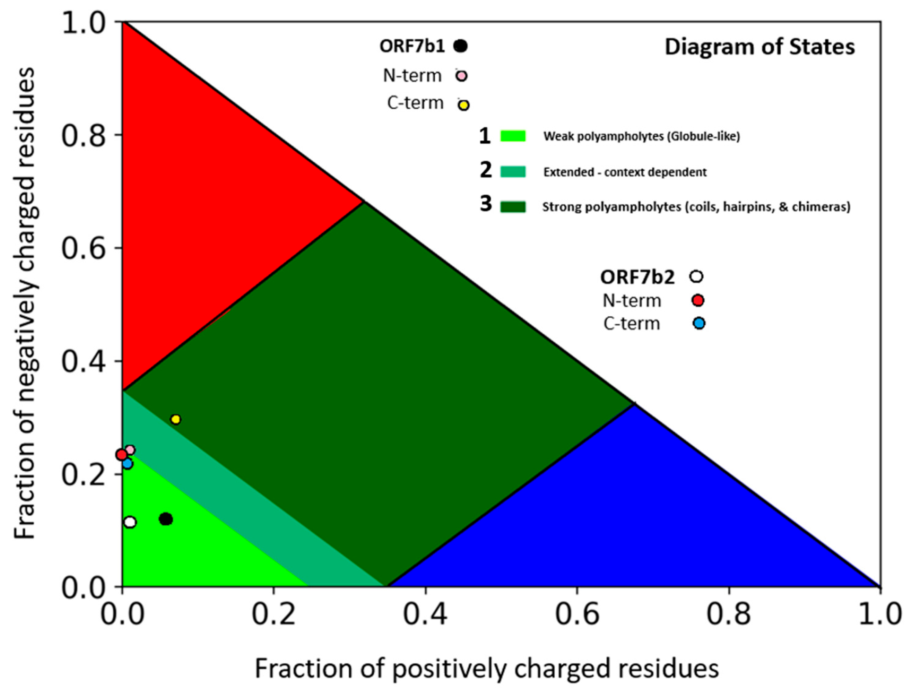
Figure 2.
Distribution of electrical charges of ORF7b2 (Top) and ORF7b1 (Bottom). NCPR, net charge distribution per residue (positive in blue and negative in red), and FCR, the fraction of charged residues. The proteins have a widespread negative surface charge, with fractions of charged residues (FCR) in both terminal segments. Both proteins show a remarkable asymmetry in their charge distribution (sigma values), with both terminal segments negatively charged. The high intensity of the charge on the tails promotes the diffusion of the negative charge over the entire structure. In fact, the charge distribution (NCPR) is on average negative for all residues.
Figure 3.
The dependence of the net charge (Z) on pH. The figure shows that, at neutral pH, ORF7b1, and ORF7b2 have negative charges (Z = −4.08 and −3.90,). Both curves remain negatively charged above pH 3 and both show a significant slope.
Figure 3.
The dependence of the net charge (Z) on pH. The figure shows that, at neutral pH, ORF7b1, and ORF7b2 have negative charges (Z = −4.08 and −3.90,). Both curves remain negatively charged above pH 3 and both show a significant slope.
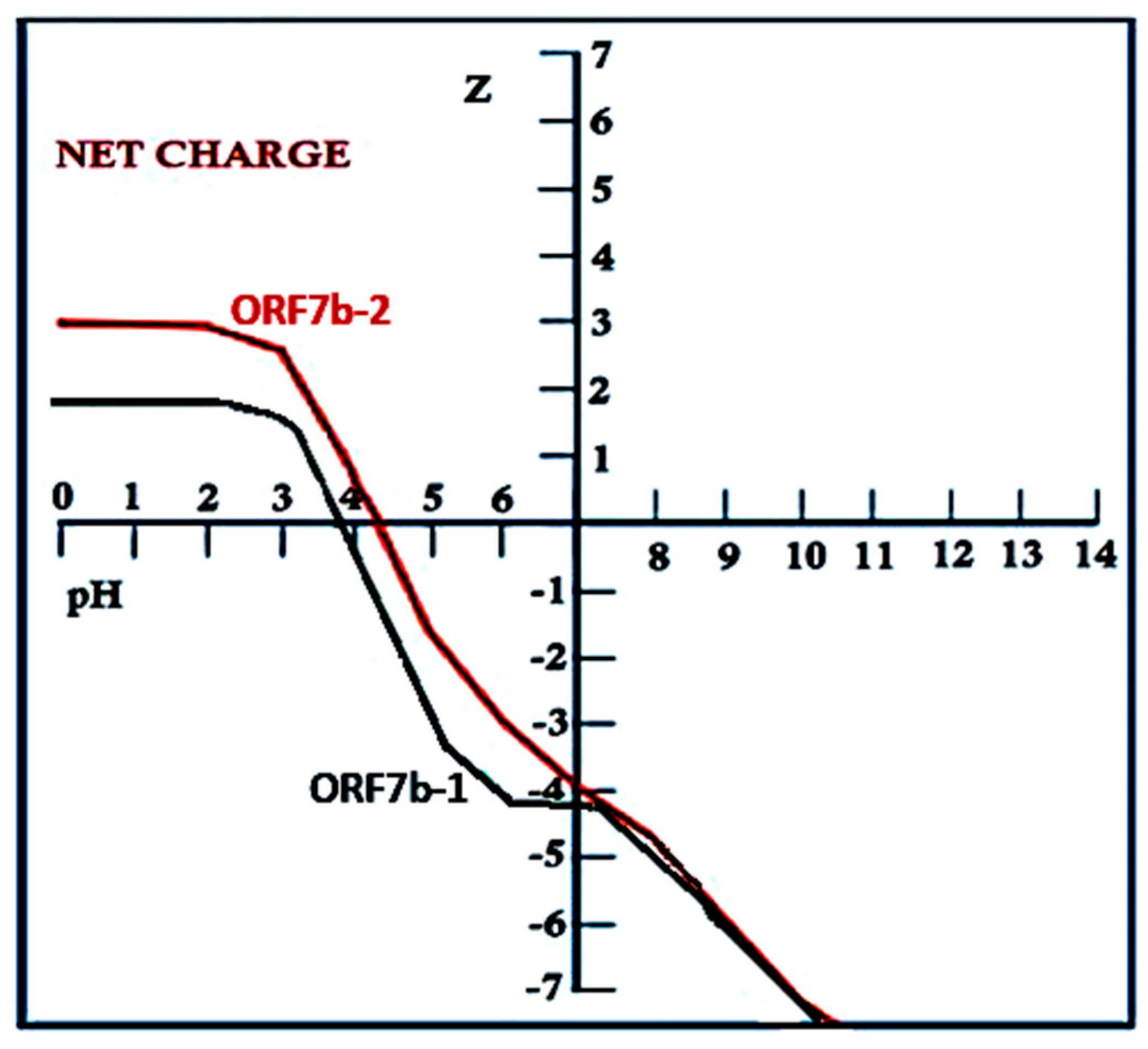
Figure 4.
Top, distribution of electrostatic surface potentials for atom of ORF7b1 (A) and ORF7b2 (B). Bottom, NPP ratio for atom of ORF7b1 (C) and ORF7b2 (D). The potential color-code accompanies both distributions in the plot. The representation is space fill. Analyzing NPP ratio models reveals more distinct polarity differences between the two molecules than simpler charge/atom models.
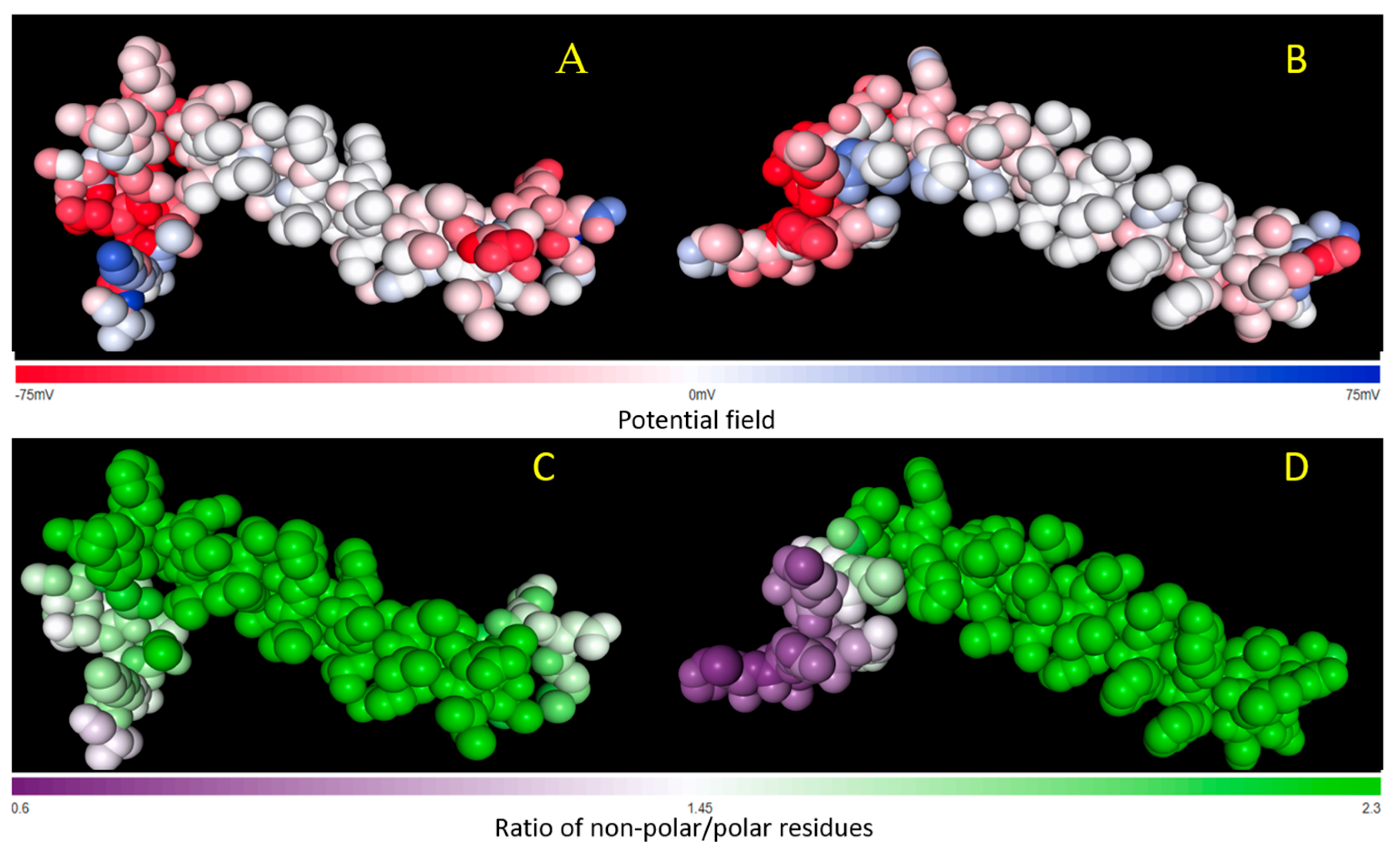
Figure 5.
Net charge distribution per residue as ionic strength and pH vary for ORF7b1 (top) and ORF7b2 (bottom). The color scales on the right show the correlation with the charge values.
Figure 5.
Net charge distribution per residue as ionic strength and pH vary for ORF7b1 (top) and ORF7b2 (bottom). The color scales on the right show the correlation with the charge values.
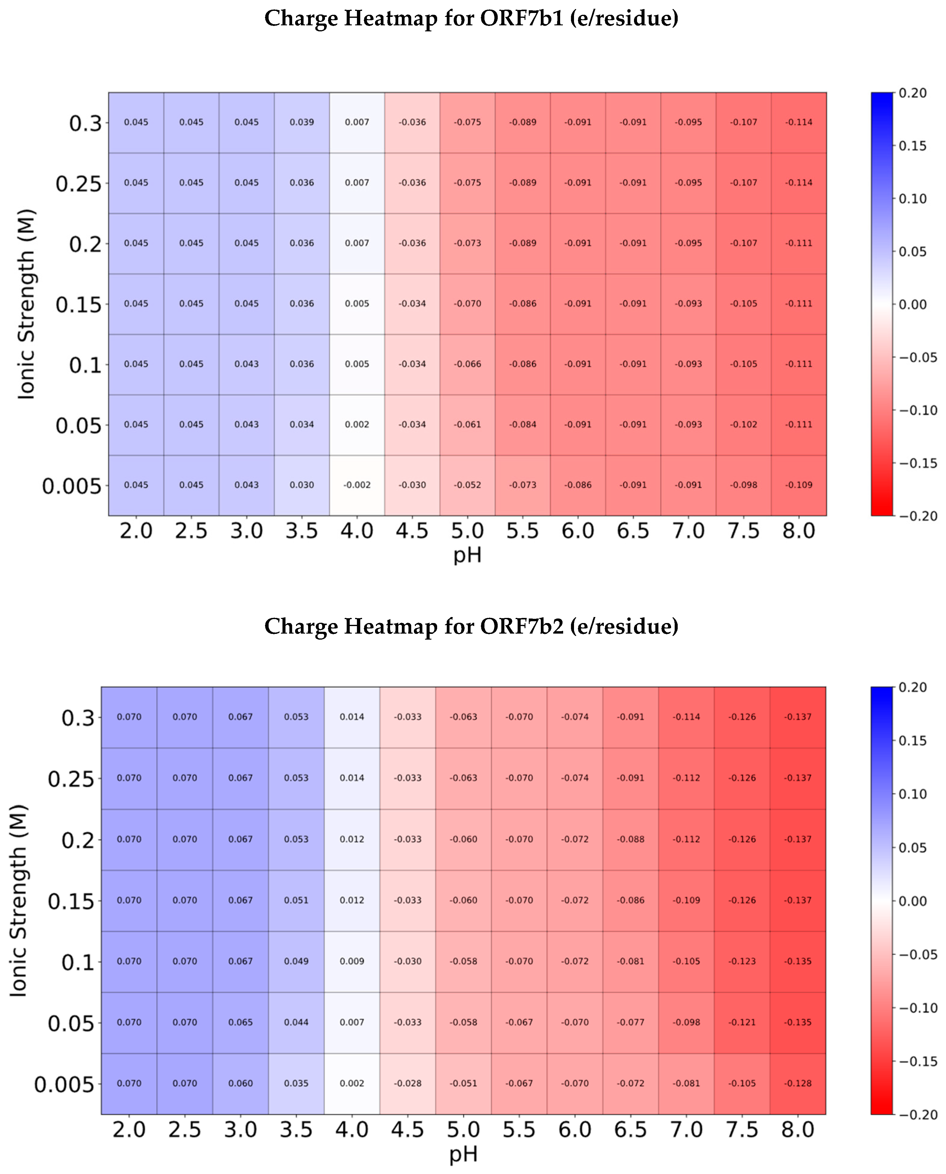
Figure 6.
Energy distribution per residue as ionic strength and pH vary for ORF7b1 (top) and ORF7b2 (bottom). The color scales on the right show the correlation with the energy values.
Figure 6.
Energy distribution per residue as ionic strength and pH vary for ORF7b1 (top) and ORF7b2 (bottom). The color scales on the right show the correlation with the energy values.
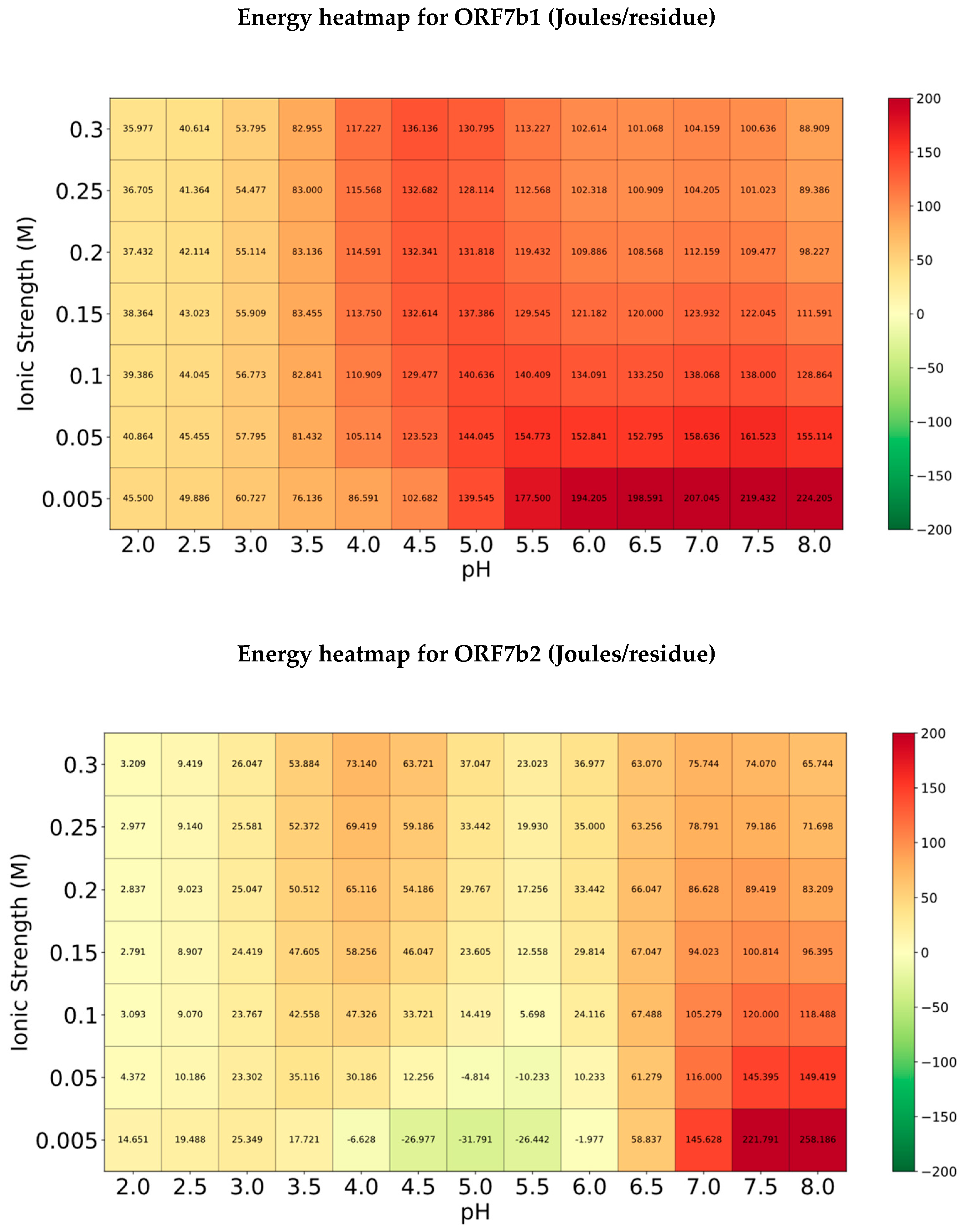
Figure 7.
The figure shows the two best models for each protein from two different structure prediction platforms, PHYRE2 and PEP-FOLD3. Both use templates to predict the central helical segments [red] and ab initio methods for the terminal segments [green]. We assume the folding process occurs at neutral pH (see supplements for details). PyMol provided structure visualization (https://pymol.org/2/).
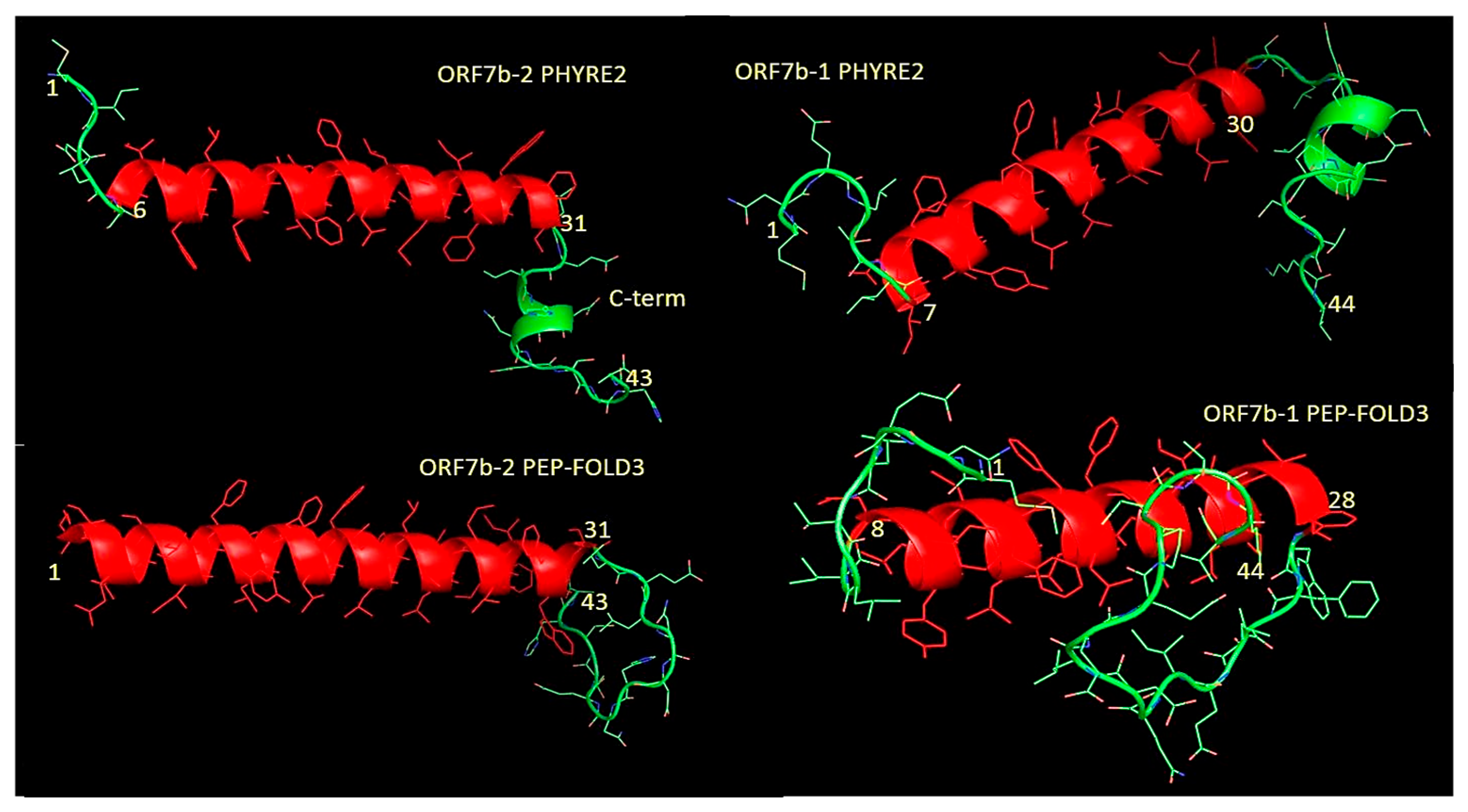
Figure 8.
The graph shows a graphical representation of the conformational probabilities (0–1) for each residue of the two proteins according to PEP-FOLD3. The graphical representation shows the probabilities [vertical axis] at each position of the sequence (horizontal axis). PEP-FOLD3 is based on the concept of structural alphabet [89], where an ensemble of elementary prototype conformations describes the whole diversity of protein structures. Each residue corresponds to the average of 4 residue. The profile uses the following color code: red: helical, green: extended, blue: coil. The graphs show in conformational terms the effect of the charges on the terminal residues of the two proteins, where at C- level is abundant the extended structure while at N-term level the coil formation.
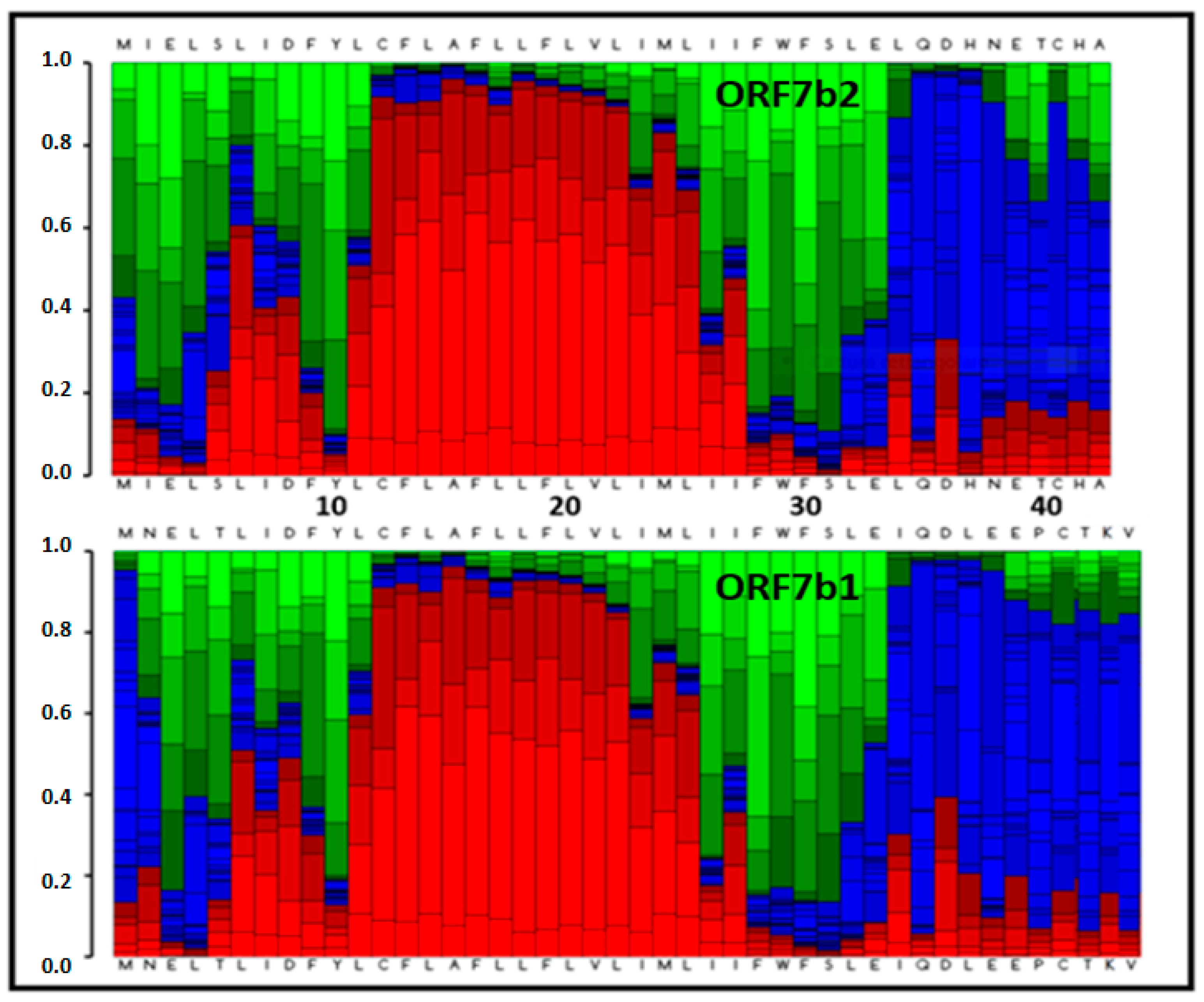
Figure 10.
The figure shows the molecular contact networks of ORF7b1 and ORF7b2, calculated by RING4. In graphs, nodes represent residues and edges represent weak molecular interactions. Obviously, the analysis does not consider the covalent bonds existing between the residues. This helps to visualize weak interactions more clearly. We evaluated the contacts through existing hydrogen bonds or van der Waals forces between residues (Table 4). In red, we have highlighted the topologically most important residues with a key role in structural coordination. The dashed bonds represent van der Waals interactions, while the solid bonds represent hydrogen bonds. The red curved line between 13Phe and 9Phe is a π-π stack. We identified these residues by calculating betweenness centrality using Cytoscape (Table 5). The lack of connection to the interaction network excludes numerous residues. We used Cytoscape to both represent these networks and the unconnected residues (Figure 11) as calculated by RING4.
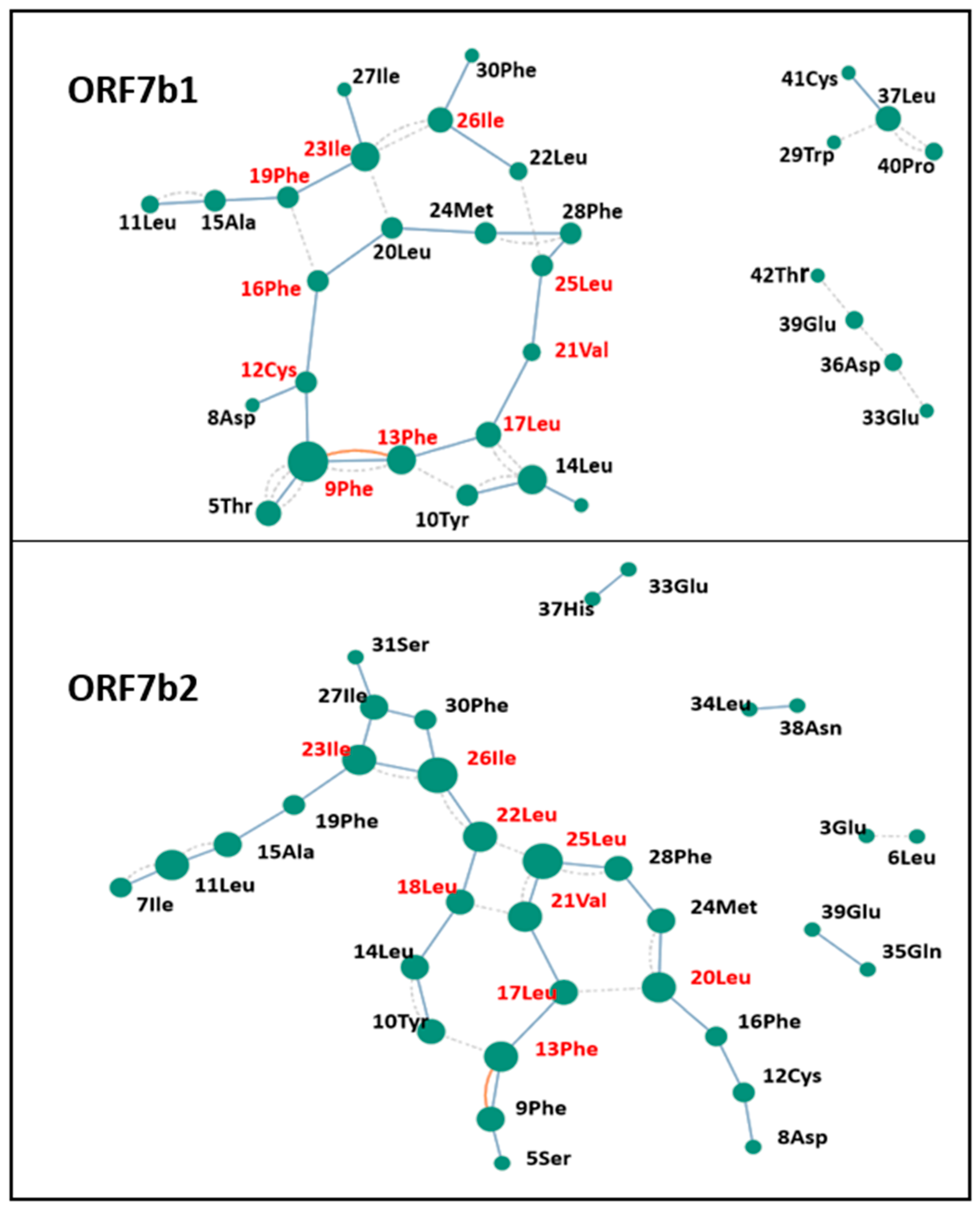
Figure 11.
ORF7b1 and 2 networks, as represented by Cytoscape. The figure also shows all the many unconnected residues of both proteins. A close view of these residues shows they are those at the terminal ends of the two molecules. This result agrees with the 3D models.
Figure 11.
ORF7b1 and 2 networks, as represented by Cytoscape. The figure also shows all the many unconnected residues of both proteins. A close view of these residues shows they are those at the terminal ends of the two molecules. This result agrees with the 3D models.
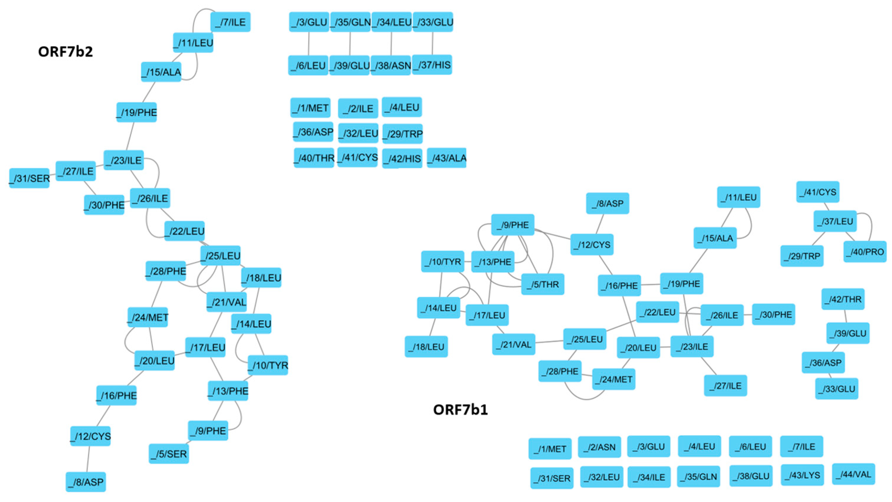
Figure 12.
Comparison of the structures of ORF7b1 and 2 with centralized residues highlighted in red. The legends within the figures report the sequences with the centralized residues in red and corresponding to those on the structure.
Figure 12.
Comparison of the structures of ORF7b1 and 2 with centralized residues highlighted in red. The legends within the figures report the sequences with the centralized residues in red and corresponding to those on the structure.
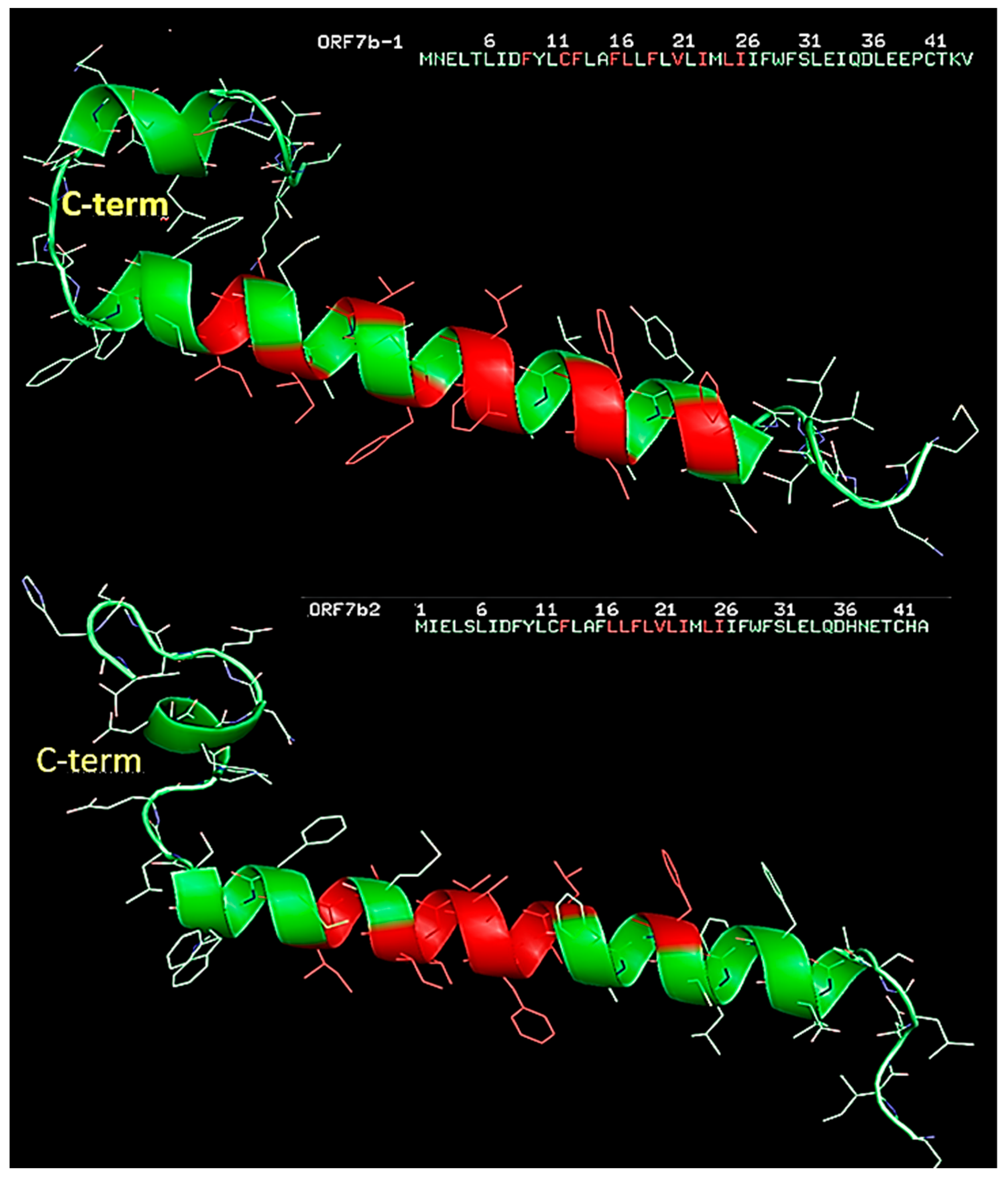
Figure 13.
Phase diagrams of ORF7b1 (top) and ORF7b2 (bottom). The force field used to calculate the predicted phase diagrams was Mpipi-GG [48]. X-Axis Scale: linear. Critical points: in red for ORF7b1 and in black for ORF7b1. Lines on the diagram represent phase boundaries, where the protein transitions from one phase to another (free protein droplets). The reduced temperature is a normalized temperature, normalized by the critical temperature of ORF7b2 sequence.
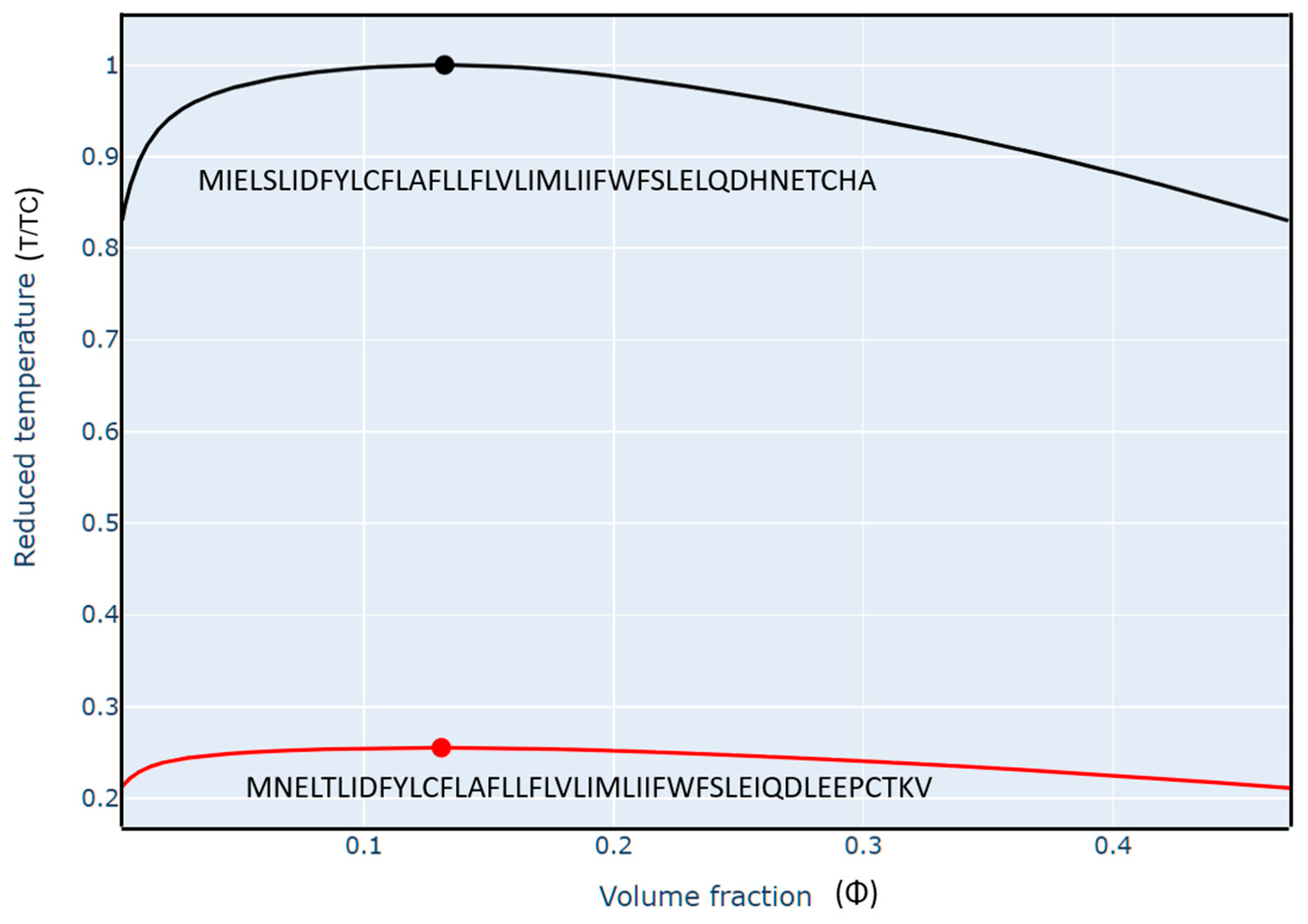
Figure 14.
Dynamics around the hinge residues of ORF7b2 (see Table 4). The model shows the hinge position with the residue number. The figures show snapshots of motions from three different views (A, B, and C) and the arrows show the series. Top: Twist movements around residues 9 and 32. Bottom: The backbone shows clear bending movements around residue 20-21.
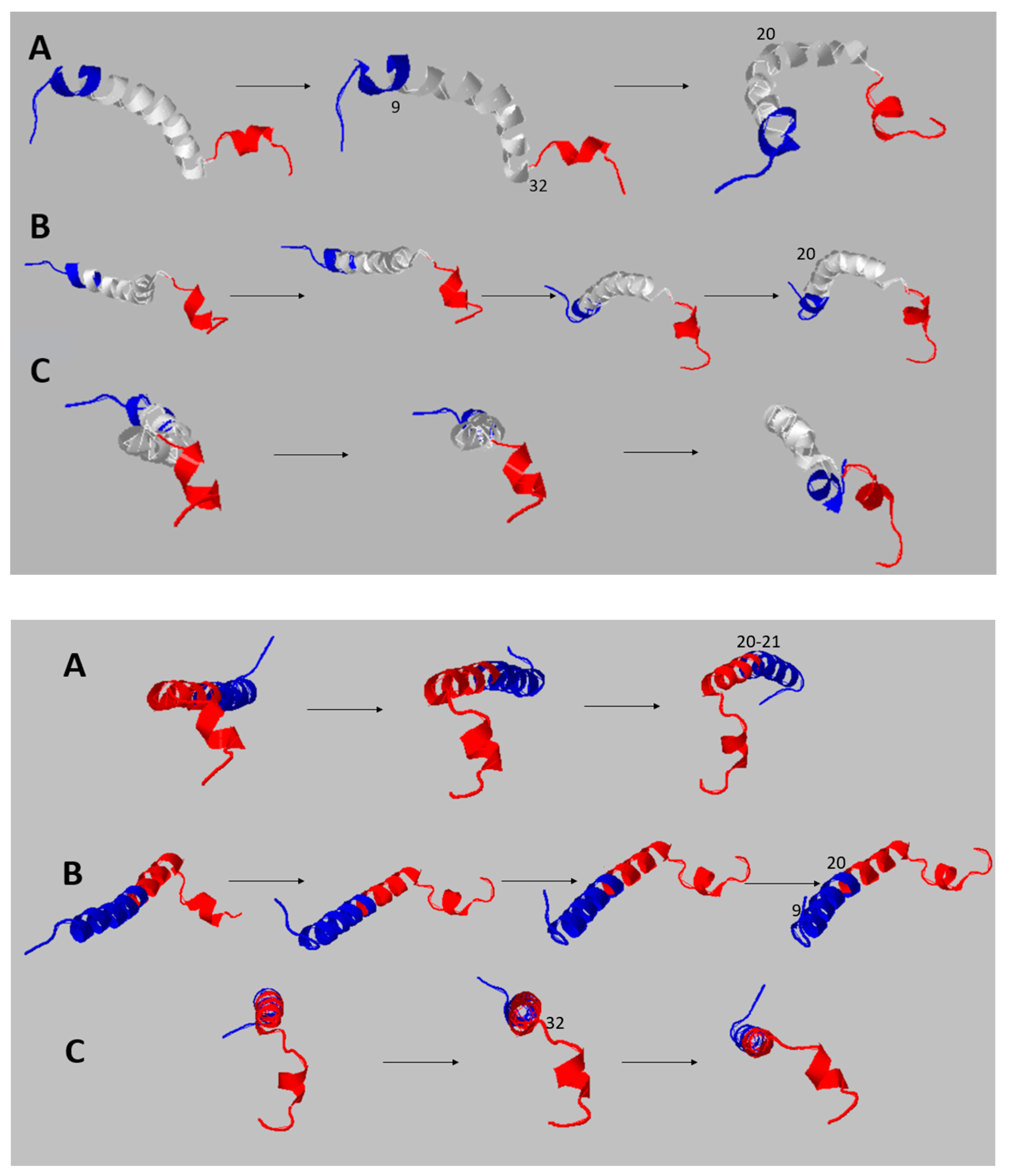
Figure 15.
Local dynamics of ORF7b2 - The superimposition of the normal modes shows us the set of local low frequency molecular movements of ORF7b2. In the upper figure, we have a side view, while in the lower figure we have a view along the major axis of the molecule. The central axis of the molecule vibrates (Figure5S) but remains quite organized, with little warping but a clear bending. In the bottom figure, both terminal segments show large fluctuations and displacements of the residues of a few tens of angstroms.
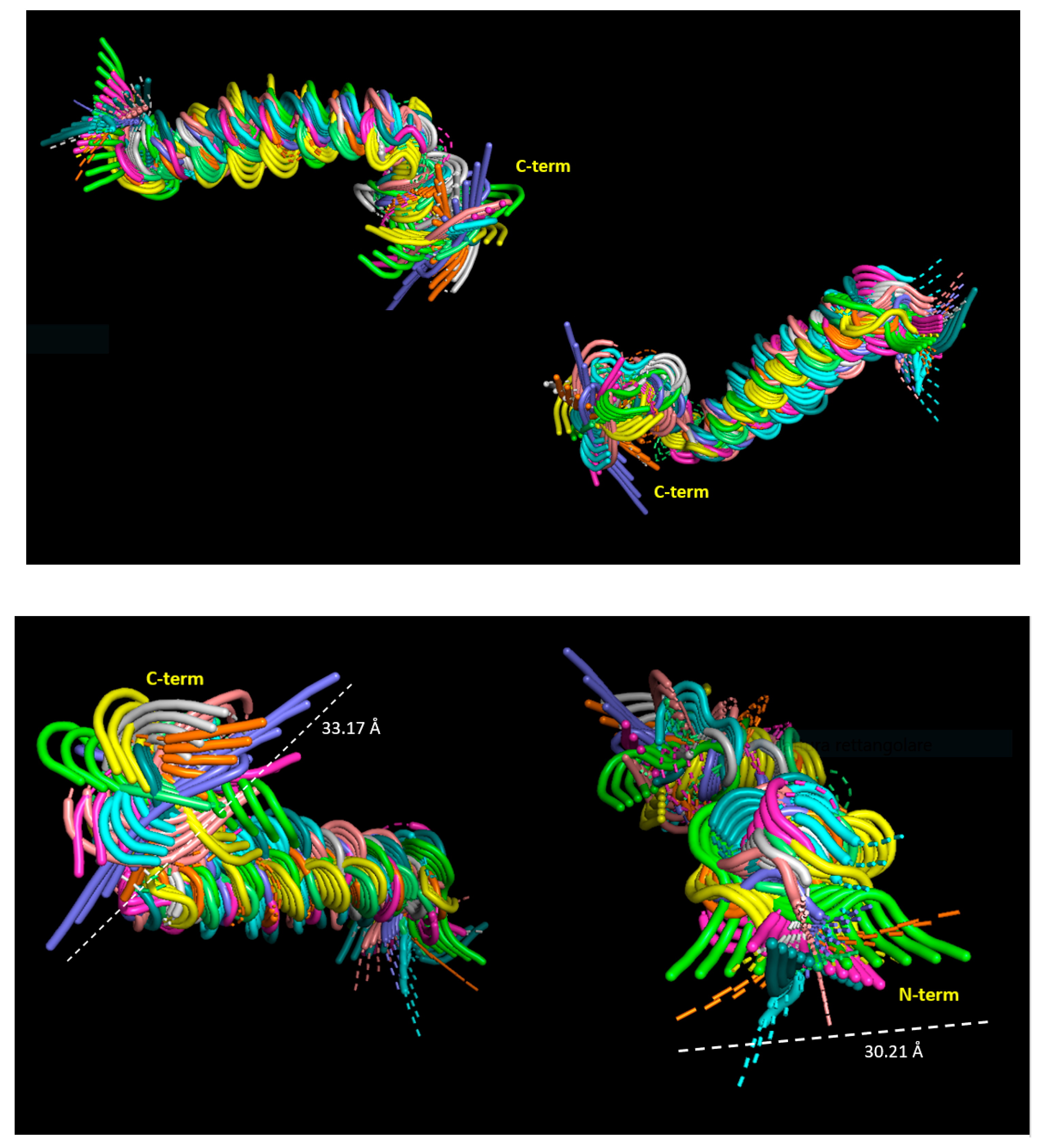
Figure 16.
The ribbon diagram of ORF7b2 shows two views from which we can appreciate the strong distortion of the dipole (red) and mass moment (greenish) vectors. The mass center is at residues 19-20. The dipole vector is not parallel to the main axis of the protein and points outwards with a tilt of 24°. Both vectors begin at the center-of-mass origin of the protein. The red dipole line’s origin aligns with the di-pole moment’s net negative charge, while its other end aligns with the net positive charge. Because the dipole is equivalent to a +0.5 charge at the N-terminus and a -0.5 charge at the C-terminus, missing positive residues at or near the C-cap end of the helix dipole destabilizes the structure because of unfavorable interactions with negative residues. This ought to make membrane insertion unstable. The distance in the figure approximates a central helix of 39.07 Å and a C-terminal movable element of 17.04 Å. Both segments will generate solids of rotation which will converge into the global prolate ellipsoid of the molecule.
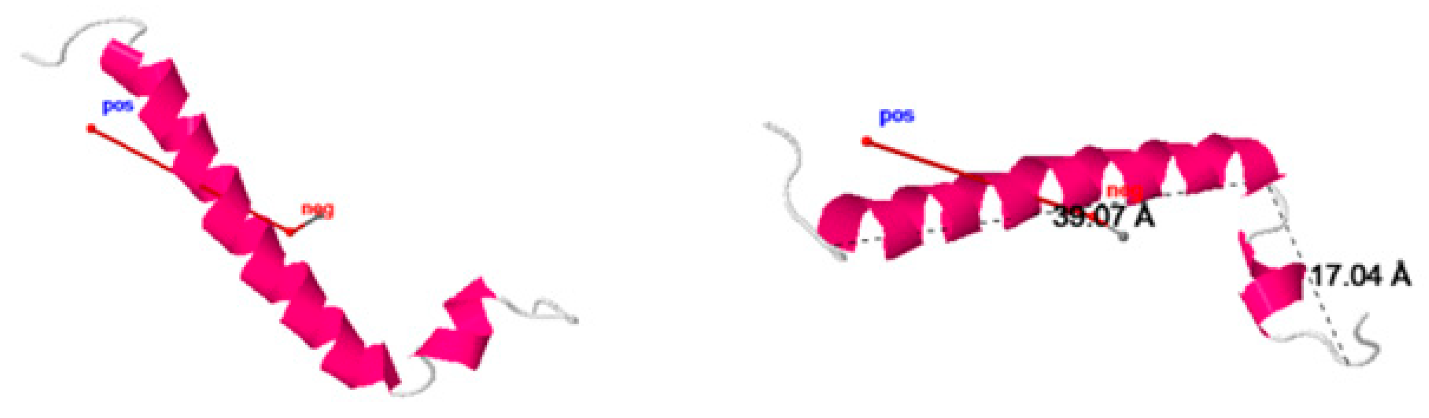
Figure 17.
Molecular dynamics of ORF7b2. The figure shows the trend of the ORF7b2 molecular dynamics simulation in water. Around 25 ns is when the Protein comes to equilibrium. The simulation shows that the protein is stable in an aqueous environment and the conformational adaptation towards the structural organization at equilibrium shows that the gradual conformational changes of settlement generate electrostatic surfaces very different from each other in terms of charge and extension. We calculated the electrostatic surfaces with DelPhi (see Methods). The small dimensions of the molecule show how even minimal conformational changes can easily reflect in variations of its electrostatic surface.
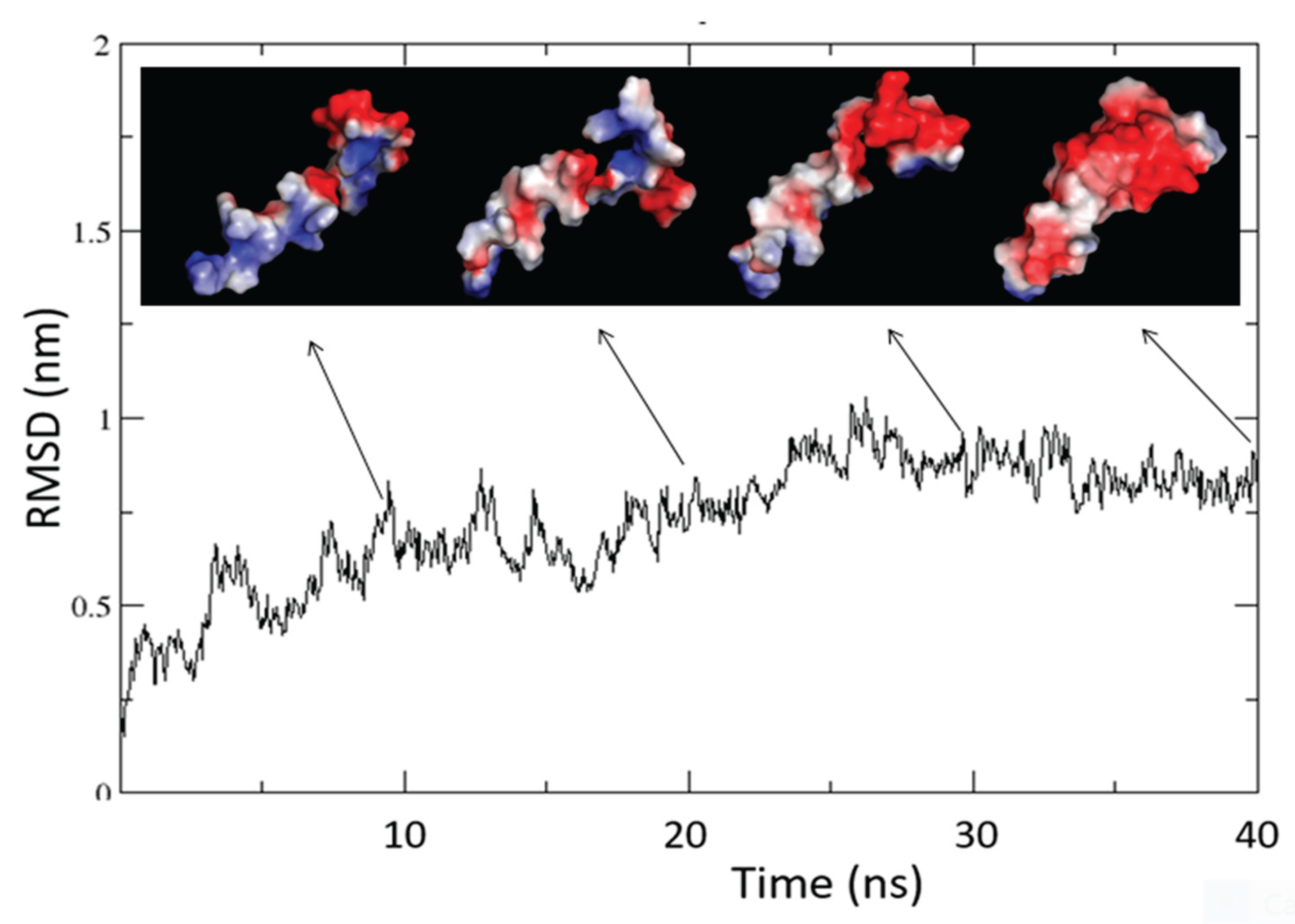
Figure 18.
The figure shows the main structural features of the ORF7b2 model got from molecular dynamics in water at neutral pH. The helix extends from L6 to W29 demonstrates bending centered on residues L17 and W21. The representation of its surface shows that the two opposite sides of the protein possess different electrostatic characteristics. A diffuse negative charge covers one side (in red) while the other side shows both charged ends (the positive charge in blue is that of the NH3+ terminal) with the central surface predominantly hydrophobic. PyMol displayed the electrostatic surfaces calculated by DelPhi.
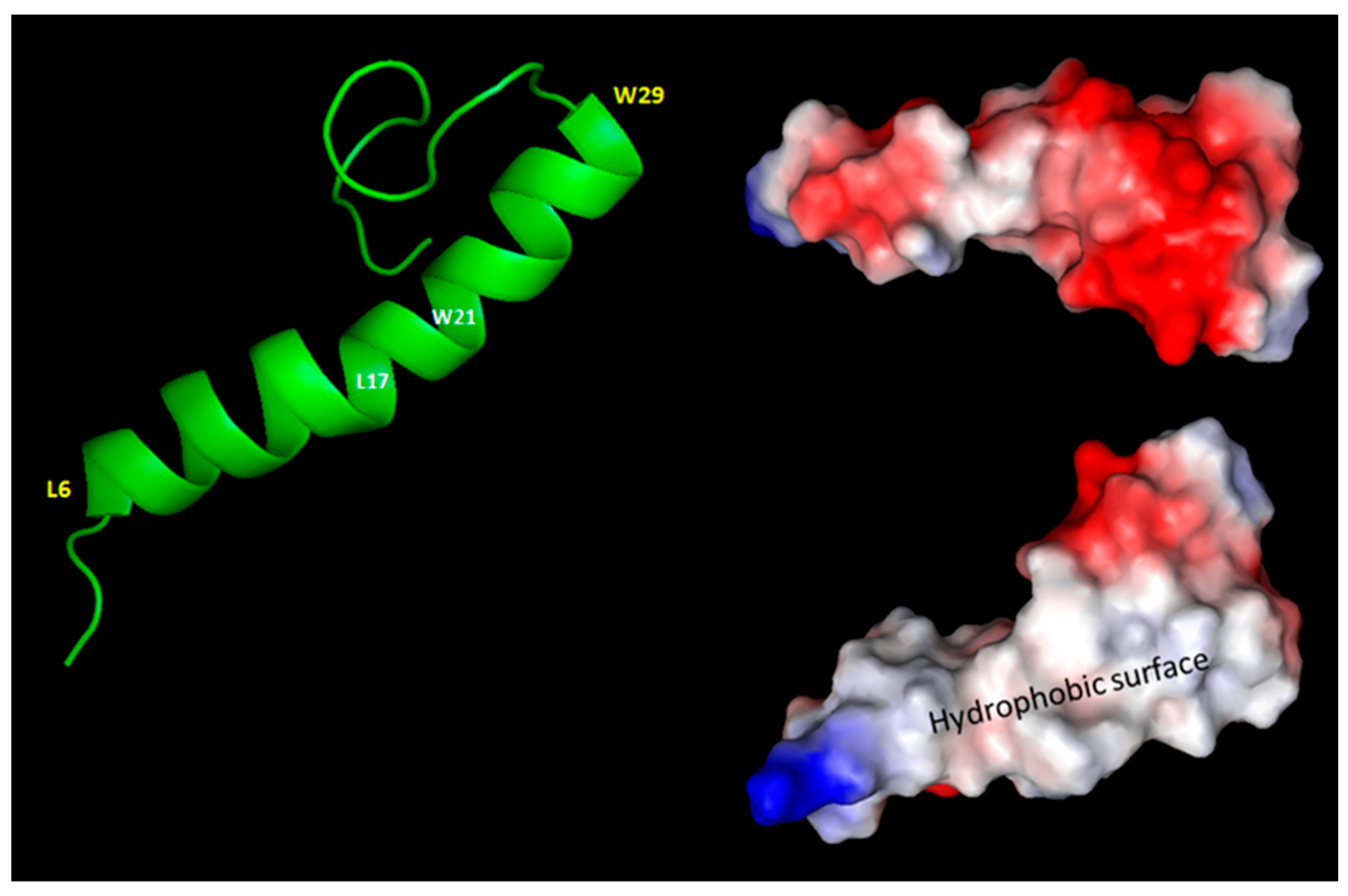
Figure 19.
The figure shows the trend of the molecular dynamics of the dimer in the membrane. For greater clarity, we show the structures at various times without the reference membrane (we presented structures inside the membrane in the Supplements). We used a model of orf7b2 dimer in parallel (cis) orientation. The graph contains as an inset the evolution of the total helicity during the 100 ns of simulation. The two graphs show in the same time interval (35—55 ns) a transition, quite super-imposable, which suggests a sudden change of structural organization with a concomitant loss of helicity and an increase in the average distance between the atoms of the global system. In a single experiment, we forced the dynamics up to 200 ns with no variation.
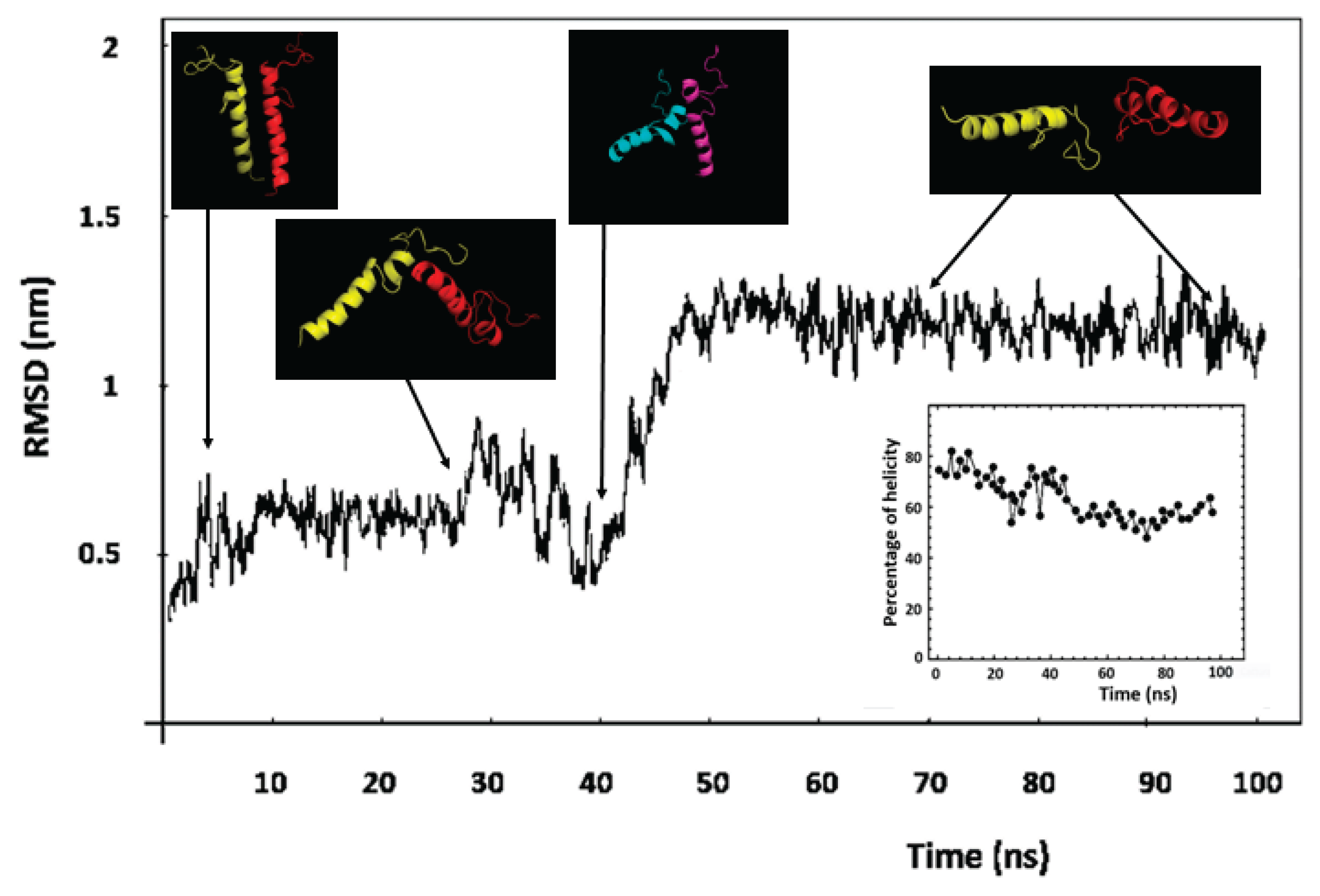

Table 1.
Amino acid composition.
| ORF7b2* | ORF7b1** | |||
|---|---|---|---|---|
| Amino acid | Number of residues | Percentage % |
Number of residues |
Percentage % |
| Ala [A] | 2 | 4.7 | 1 | 2.3 |
| Asn [N] | 1 | 2.3 | 1 | 2.3 |
| Asp [D] | 2 | 4.7 | 2 | 4.5 |
| Cys [C] | 2 | 4.7 | 2 | 4.5 |
| Gln [Q] | 1 | 2.3 | 1 | 2.3 |
| Glu [E] | 3 | 7.0 | 4 | 9.1 |
| His [H] | 2 | 4.7 | - | - |
| Ile [I] | 5 | 11.6 | 5 | 11.4 |
| Leu [L] | 11 | 25.6 | 11 | 25.0 |
| Lys [K] | - | - | 1 | 2.3 |
| Met [M] | 2 | 4.7 | 2 | 4.5 |
| Phe [F] | 6 | 14.0 | 6 | 13.6 |
| Pro [P] | - | - | 1 | 2.3 |
| Ser [S] | 2 | 4.7 | 1 | 2.3 |
| Thr [T] | 1 | 2.3 | 2 | 4.5 |
| Trp [W] | 1 | 2.3 | 1 | 2.3 |
| Tyr [Y] | 1 | 2.3 | 1 | 2.3 |
| Val [V] | 1 | 2.3 | 2 | 4.5 |
Note: Negative residues are in red; positive residues are in blue. *Total number of negatively charged residues (Asp + Glu): 5, and of positively charged residues (Arg + Lys): 0 ** Total number of negatively charged residues (Asp + Glu): 6, and of positively charged residues (Arg + Lys): 1. Both proteins lack glycine and ORF7b1 shows a proline. Computed data came from ProtParam (Expasy; https://web.expasy.org/protparam/).
Table 2.
Protein Sequence.
| Protein | Sequence 5 10 15 20 25 30 35 40 |
|---|---|
| ORF7b-2 | MIELSLID FYLCFLAFLLFLVLIMLIIFWF SLELQDHNETCHA |
| ORF7b-1 | MNELTLID FYLCFLAFLLFLVLIMLIIFWF SLEIQDLEEPCTKV |
Note: The residues in red have a significant statistical propensity for the alpha-helix, those in green for the coil, and those in blue for the extended structure [69]. The 21 residues in larger characters (from 9 to 30) are those supposed to be helical and transmembrane. Therefore, the first 8-9 residues and the last 14-15 residues of both proteins should be involved in the terminal segments. In the whole molecule only 46% of the residues have a helical propensity and, in the helix, shown as trans-membrane, out of 20 residues only 9 have an adequate helical propensity. The two proteins show an identical 9-29 sequence. A visual analysis of the N-terminal sequences of both shows the lack of any signal sequences (translocon sequence). Signal sequences are N-terminal extensions of the nascent polypeptides (pre-proteins) of secretory and membrane proteins. They are of about 15-30 amino acid residues and comprised a positively charged N-terminal region with the cleavage site for signal peptidase (Ala-X-Ala motif at the C-terminal end of the signal peptide). Therefore, both proteins do not show the features [77] essential for entry into the ER.
Table 3.
Charge distribution analysis of ORF7b1 and ORF7b2.
| Physical-chemical parameters | ORF7b1 | ORF7b2 | Notes |
|---|---|---|---|
| N [MW] | 44 (Mw. 5301.51) | 43 (Mw.5179.31) | Number of residues and M.W. |
| f- | 0.13636 | 0.11628 | Fraction of negative residues |
| f+ | 0.02273 | 0.00000 | Fraction of positive residues |
| FCR | 0.15909 | 0.11628 | Fraction of charged residues |
| NCPR | -0.11364 | -0.11628 | Net charge per residue |
| Sigma | 0.08117 | 0.11628 | Charge asymmetry |
| Delta | 0.03182 | 0.01706 | square deviation of every blob σ value from the sequence’s mean σ value. |
| Max Delta | 0.08945 | 0.06725 | δ value associated with the segregated sequence of the charge composition provided. |
| pI | 3.72 | 4.32 | Isoelectric point at pH 7.00 |
| AH | -0.83 | -0.98 | Average hydrophilicity |
|
Phase Plot (Region) |
1 | 1 | (See the state diagram) |
|
Phase Plot Annotation |
Globule/Tadpole | Globule/Tadpole | Prolate elongated structures |
| Polymeric State | (Weak negative polyampholyte) | (Weak negative polyampholyte) |
We evaluated the protein’s charge distribution according to Das and Pappu [36,37]. We calculated the fraction of charged residues as FCR = |f+ + f-|, and the net charge per residue (NCPR) as |f+ - f-|. In this context, f+ and f- represent the fraction of positive and negative charges. Sigma, σ = [f+ - f-]/[f+ + f-], where f- and f+ refer to the fraction of negative and positive residues across the entire sequence and sigma their distribution symmetry. These values allow classifying the behavioral tendency in solution of the segmental sequences of protein into distinct regions of the Diagram of States for IDPs. We calculated the pI according to Lukasz et al. [81] and AH according to Kyte and Doolitle [70].
Table 4.
Molecular contacts calculated by RING4 for the ORF7b2 and ORF7b1 models.
| ORF7b2 | ORF7b1 | ||||||||
|---|---|---|---|---|---|---|---|---|---|
| H-bond | van der Waals | H-bond | van der Waals | ||||||
| Source | Target | Seq | Source | Target | Source | Target | Seq | Source | Target |
| 3 | 3/GLU | 6/LEU | 5/THR | 9/PHE | 5 | 5/THR | 9/PHE | ||
| 5/SER | 9/PHE | 5 | 6 | 6/LEU | 10/TYR | ||||
| 6 | 6/LEU | 9/PHE | 7/ILE | 11/LEU | 7 | ||||
| 7/ILE | 11/LEU | 7 | 7/ILE | 11/LEU | 8 | 8/ASP | 12/CYS | ||
| 8/ASP | 12/CYS | 8 | 9/PHE | 12/CYS | 9 | 9/PHE | 13/PHE | ||
| 9/PHE | 13/PHE | 9 | 9/PHE | 13/PHE | - | ||||
| 10/TYR | 14/LEU | 10 | 10/TYR | 13/PHE | 10/TYR | 14/LEU | 10 | 10/TYR | 13/PHE |
| 10/TYR | 14/LEU | 10/TYR | 14/LEU | ||||||
| 11/LEU | 15/ALA | 11 | 11/LEU | 15/ALA | 11/LEU | 15/ALA | 11 | 11/LEU | 15/ALA |
| 12/CYS | 16/PHE | 12 | 12/CYS | 16/PHE | 12 | ||||
| 13/PHE | 17/LEU | 13 | 13/PHE | 17/LEU | 13 | 13/PHE | 16/PHE | ||
| 14/LEU | 17/LEU | 14 | 14/LEU | 18/LEU | 14 | 14/LEU | 17/LEU | ||
| 14/LEU | 18/LEU | - | 15/ALA | 18/LEU | 15 | 15/ALA | 18/LEU | ||
| 15/ALA | 18/LEU | 15 | 15/ALA | 19/PHE | |||||
| 15/ALA | 19/PHE | - | 16 | 16/PHE | 19/PHE | ||||
| 16/PHE | 20/LEU | 16 | 16/PHE | 20/LEU | |||||
| 17/LEU | 21/VAL | 17 | 17/LEU | 20/LEU | 17/LEU | 21/VAL | 17 | ||
| 18/LEU | 22/LEU | 18 | 18/LEU | 21/VAL | 18/LEU | 22/LEU | 18 | ||
| - | 19/PHE | 23/ILE | 19 | ||||||
| 19/PHE | 23/ILE | 19 | 20/LEU | 24/MET | 20 | 20/LEU | 23/ILE | ||
| 20/LEU | 23/ILE | 20 | 20/LEU | 24/MET | 21/VAL | 25/LEU | 21 | ||
| 20/LEU | 24/MET | - | 22/LEU | 26/ILE | 22 | 22/LEU | 25/LEU | ||
| 21/VAL | 25/LEU | 21 | 21/VAL | 25/LEU | 23/ILE | 26/ILE | 23 | 23/ILE | 26/ILE |
| 22/LEU | 26/ILE | 22 | 22/LEU | 25/LEU | 23/ILE | 27/ILE | |||
| - | 22/LEU | 26/ILE | 24/MET | 27/ILE | 24 | 24/MET | 27/ILE | ||
| 23/ILE | 26/ILE | 23 | 23/ILE | 26/ILE | 24/MET | 28/PHE | 24/MET | 28/PHE | |
| 23/ILE | 27/ILE | - | 25/LEU | 28/PHE | 25 | ||||
| - | 25/LEU | 29/TRP | |||||||
| 24/MET | 28/PHE | 24 | 26/ILE | 29/TRP | 26 | 26/ILE | 29/TRP | ||
| 25/LEU | 28/PHE | 25 | 25/LEU | 22/LEU | 26/ILE | 30/PHE | |||
| 25/LEU | 29/TRP | - | 25/LEU | 28/PHE | 27 | 27/ILE | 30/PHE | ||
| 26/ILE | 30PHE | 26 | 28/PHE | 31/SER | 28 | ||||
| 27/ILE | 30/PHE | 27 | 29 | 29/TRP | 37/LEU | ||||
| 27/ILE | 31/SER | - | 33/GLU | 36/ASP | 33 | 33/GLU | 36/ASP | ||
| 28/PHE | 32/LEU | 28 | 28/PHE | 31/SER | 33/GLU | 37/LEU | 33/GLU | 37/LEU | |
| 33/GLU | 37/HIS | 33 | 34 | 34/ILE | 38/GLU | ||||
| 34/LEU | 38/ASN | 34 | 34/LEU | 38/ASN | 36/ASP | 39/GLU | 36 | ||
| 35/GLN | 38/ASN | 35 | 35/GLN | 38/ASN | 37/LEU | 41/CYS | 37 | 37/LEU | 40/PRO |
| 35/GLN | 39/GLU | - | |||||||
Note: The table reports the pairs of residues interacting with H-bond and van der Waals as molecular contacts for ORF7b1 and 2. The table shows in red the residues that show a high degree (Hub) and a high centrality, according to Table 5.
Table 5.
Calculated topological values for the RIN ORF7b2 and ORFb1 models.
| ORF7b2 | ORF7b1 | ||||
|---|---|---|---|---|---|
| Betweenness centrality |
Degree | Residue | Betweenness centrality |
Degree | Residue |
| 276.3333 | 4.0 | 22/LEU | 142.3337 | 3.0 | 12/CYS |
| 261.0 | 5.0 | 26/ILE | 140.3377 | 3.0 | 16/PHE |
| 194.0 | 4.0 | 23/ILE | 126.3338 | 8.0 | 9/PHE |
| 187.6666 | 3.0 | 17/LEU | 117.0 | 5.0 | 23/ILE |
| 155.9999 | 4.0 | 21/VAL | 107.0 | 3.0 | 19/PHE |
| 148.1666 | 5.0 | 25/LEU | 104.0001 | 4.0 | 17/LEU |
| 143.1666 | 4.0 | 20/LEU | 103.0 | 5.0 | 13/PHE |
| 142.4999 | 3.0 | 18/LEU | 99.66660 | 3.0 | 25/LEU |
| 126.0 | 2.0 | 19/PHE | 92.0 | 4.0 | 26/ILE |
| 92.1666 | 4.0 | 13/PHE | 84.66070 | 2.0 | 21/VAL |
| 88.0 | 3.0 | 15/ALA | 65.66667 | 3.0 | 20/LEU |
| 88.0 | 2.0 | 16/PHE | 64.0 | 2.0 | 22/LEU |
| 56.0 | 3.0 | 28/PHE | 49.66666 | 5.0 | 14/LEU |
| 51.0 | 3.0 | 27/ILE | 42.0 | 3.0 | 15/ALA |
| 48.3333 | 3.0 | 14/LEU | 31.33333 | 3.0 | 24/MET |
| 46.0 | 4.0 | 11/LEU | 25.66644 | 3.0 | 28/PHE |
| 46.0 | 3.0 | 9/PHE | 19.33332 | 3.0 | 10/TYR |
| 46.0 | 2.0 | 12/CYS | 6.0 | 4.0 | 37/LEU |
| 43.1666 | 3.0 | 24/MET | 4.0 | 2.0 | 36/ASP |
| 34.5767 | 3.0 | 10/TYR | 4.0 | 2.0 | 39/GLU |
| 34.0 | 2.0 | 30/PHE | 0.0 | 1.0 | 29/TRP |
| 0.0 | 2.0 | 7/ILE | 0.0 | 2.0 | 40/PRO |
| 0.0 | 1.0 | 3/GLU | 0.0 | 1.0 | 41/CYS |
| 0.0 | 1.0 | 5/SER | 0.0 | 1.0 | 33/GLU |
| 0.0 | 1.0 | 6/LEU | 0.0 | 1.0 | 42/THR |
| 0.0 | 1.0 | 8/ASP | 0.0 | 1.0 | 8/ASP |
| 0.0 | 1.0 | 31/SER | 0.0 | 1.0 | 27/ILE |
| 0.0 | 1.0 | 33/GLU | 0.0 | 4.0 | 5/THR |
| 0.0 | 1.0 | 34/LEU | 0.0 | 1.0 | 30/PHE |
| 0.0 | 1.0 | 35/GLN | 0.0 | 2.0 | 11/LEU |
| 0.0 | 1.0 | 37/HIS | 0.0 | 1.0 | 18/LEU |
| 0.0 | 1.0 | 38/ASN | 0.0 | 0.0 | 1/MET |
| 0.0 | 1.0 | 39/GLU | 0.0 | 0.0 | 2/ASN |
| 0.0 | 0.0 | 1/MET | 0.0 | 0.0 | 3/GLU |
| 0.0 | 0.0 | 2/ILE | 0.0 | 0.0 | 31/SER |
| 0.0 | 0.0 | 4/LEU | 0.0 | 0.0 | 32/LEU |
| 0.0 | 0.0 | 29/TRP | 0.0 | 0.0 | 34/ILE |
| 0.0 | 0.0 | 32/LEU | 0.0 | 0.0 | 35/GLN |
| 0.0 | 0.0 | 36/ASP | 0.0 | 0.0 | 38/GLU |
| 0.0 | 0.0 | 40/THR | 0.0 | 0.0 | 4/LEU |
| 0.0 | 0.0 | 41/CYS | 0.0 | 0.0 | 43/LYS |
| 0.0 | 0.0 | 42/HIS | 0.0 | 0.0 | 44/VAL |
| 0.0 | 0.0 | 43/ALA | 0.0 | 0.0 | 6/LEU |
| 0.0 | 0.0 | 7/ILE | |||
Note: Betweenness centrality measures the extent to which a vertex lies on paths between other vertices. Vertices with high betweenness may have considerable influence within a network by their control over information passing between others. A common method is to select around the 20% of nodes that are at the top of the betweenness centrality values [104]. We selected the top 9 (21%) and 10 (22.7%). Selected nodes are in red.
Table 6.
ORF7b2 hinge residues.
| The slowest mode 1 | |||
|---|---|---|---|
| Rigid Part No | Residues | Score | Hinge residues |
| 1 | 1-20 | 0.88 | 20 |
| 2 | 21-43 | 0.9 | 20 |
| The slowest mode 2 | |||
| Rigid Part No | |||
| 1 | 1-9 | 0.68 | 9 |
| 2 | 10-32 | 0.82 | 32 |
| 3 | 33-43 | 0.85 | 32 |
The table shows the best hinge residues in the ORF7-b2 structure and the reliability of the result as calculated by HINGE-Prot [the score varies between 0 and 1]. These residues define twist angles or points of rigidity that organize moving the entire structure (see also Figure 14).
Disclaimer/Publisher’s Note: The statements, opinions and data contained in all publications are solely those of the individual author(s) and contributor(s) and not of MDPI and/or the editor(s). MDPI and/or the editor(s) disclaim responsibility for any injury to people or property resulting from any ideas, methods, instructions or products referred to in the content. |
© 2025 by the author. Licensee MDPI, Basel, Switzerland. This article is an open access article distributed under the terms and conditions of the Creative Commons Attribution (CC BY) license (https://creativecommons.org/licenses/by/4.0/).
Copyright: This open access article is published under a Creative Commons CC BY 4.0 license, which permit the free download, distribution, and reuse, provided that the author and preprint are cited in any reuse.


