
Submitted:
17 April 2023
Posted:
17 April 2023
You are already at the latest version
Abstract
The Direction-of-Arrival (DoA) estimation methods are highly versatile and find extensive applications in satellite communication. The DoA methods are employed across a range of orbits, from Low Earth Orbits (LEO) to Geostationary Earth Orbits (GEO). They serve multiple applications, including altitude determination, geolocation and estimation accuracy, target localization, and relative and collaborative positioning. This paper presents a novel approach for modeling the DoA angle using a closed-form expression, incorporating the boresight angle and satellite and Earth station position data. The method uses the geographic coordinate system in the satellite communication system, precisely the latitude and longitude of the Earth station and altitude parameters of the satellite stations, to calculate the Earth station’s elevation angle and accurately model the DoA angle. Furthermore, this paper performs a comprehensive comparative analysis of various DoA methods to gain deeper insights into the performance of DoA estimation in multi-antenna systems operating under spatially correlated channels. Accordingly, this paper evaluates DoA estimation performance using root-mean-square-error (RMSE) statistics for uplink and downlink conditions through extensive Monte Carlo simulations. The simulation’s effectiveness is validated against the Cramer-Rao Bound (CRB) performance metric for the Additive white Gaussian noise (AWGN) case. (i.e., thermal noise). The simulation results demonstrate improved RMSE performance in satellite systems by incorporating spatial correlation into the system model.
Keywords:
Direction of Arrival (DoA) Estimation
; Multipath Environment
; Geostationary Earth Orbit (GEO)
; Low Earth Orbit (LEO)
; and Spatial Correlation
1. Introduction
Accurate estimation of Direction of Arrival (DoA) is a constantly evolving research area with broad applications in multiple communication technologies, including but not limited to radar, sonar, cellular, geophysics, acoustic tracking, and astronomy. These applications span numerous fields, such as military, satellite, vehicular, and more [1]. In satellite communication systems, the DoA-based measurements for locating objects of interest, such as ground signal sources or vice versa, have become increasingly important in recent years [2]. The communication between ground and space segments in satellite systems is established through basic parameters such as frequencies and orbits [3]. In general, the satellite orbits are ellipses within the orbital plane, but in the case of zero eccentricity, they are considered circular orbits [3]. Satellite altitude can vary significantly, from Low Earth Orbits (LEO) at heights of 180-2,000 km to Geostationary Earth Orbits (GEO) at approximately 35,786 km above the Earth’s surface [4].
The DoA estimation methods have been extensively researched for satellite communication systems, as these methods have unique strengths and weaknesses concerning their techniques, speed, computational complexities, accuracy, and channel characteristics [5]. Consequently, DoA estimation methods find a wide range of applications in satellite communication systems, such as altitude determination [6], geolocation accuracy [7,8], estimation accuracy [9], target localization [10], relative positioning [11], and collaborative positioning [12]. Thus, to improve DoA estimation performance and reduce errors, which, in turn, improves communication system performance and accuracy, accurate satellite channel modeling is essential.
This paper proposes a novel approach to model the DoA angle using closed-form expressions based on the boresight angle, and satellite and ground station position data. Consequently, this approach utilizes the geographic coordinate system (i.e., latitude and longitude of the Earth station) and the satellite stations’ altitude parameters to calculate the Earth station’s elevation angle and accurately model the DoA angle. Multiple DoA techniques were evaluated to gain insight into the performance of DoA estimation in multi-antenna systems operating under spatially correlated channels. A thorough comparative analysis was performed to gauge the effectiveness of a single-receiver system with multiple antennas under different channel impairments for various DoA techniques. The above investigations into DoA estimation performance are still not explored in the literature. The estimation performance is evaluated using Root Mean Square Error (RMSE) measurements for uplink and downlink conditions.
The paper is outlined as follows: Section 2 reviews the challenges in DoA estimation methods for satellite communication and addresses the importance of an accurate satellite channel model. Section 3 delves into the satellite geometries for DoA estimation in both uplink and downlink scenarios for two different satellite systems, i.e., GEO and LEO satellites. For uplink communication, the study utilized spherical geometries to determine the satellite’s look angles and range, whereas for downlink communication, basic geometries were employed for satellites. Section 4 presents the signal model for both uplink and downlink scenarios for the aforementioned satellite systems. Notably, for LEO satellite systems, additional parameters, such as the satellite’s altitude, velocity, and Doppler shift (due to the satellite’s motion), were taken into account.
In Section 5, two DoA estimation techniques are outlined: the classical Delay and Sum (DAS) method and the subspace-based Multiple Signal Classification (MUSIC) algorithms [5]. The aim is to assess the ability of different DoA estimation techniques to accurately estimate the DoA in a multiple antennas based receiver system while operating under diverse channel impairments. The limitations that are examined in this paper comprise Additive White Gaussian Noise (AWGN) i.e., thermal noise, Envelope fading corresponding from a Rice channel with channel-phase random variables [13], and spatial correlation in multi-antenna element systems [14]. The efficacy of the proposed technique is evaluated through comprehensive Monte Carlo simulations in MATLAB. To validate the precision of the simulations, Section 6 presents the Cramer-Rao Lower Bound (CRLB) as a performance measure for the AWGN scenario. Section 7 provides a detailed analysis of the numerical outcomes. Finally, Section 8 summarizes the key findings of this study.
2. Related Works
This section explores the existing literature on DoA estimation methods in the context of satellite communication systems, considering various factors that may affect efficient communication. It also discusses the crucial aspects of accurately modeling the satellite channel and compares the findings of this study with the literature.
The estimation of DoA is a topic of considerable interest in the field of satellite communication systems. Its investigation has been extensive, with researchers exploring a variety of scenarios and confronting a multitude of practical challenges. Among these challenges are accurate Angle of Arrival (AoA) estimation, optimization of positioning accuracy in the presence of system failures, resolution of phase measurement ambiguities, and geolocation accuracy for moving objects. Each of these challenges has been tackled by researchers, who have provided valuable insights and potential solutions. An example of a study to accurately estimate the Angle of Arrival (AoA) is presented in [9], where the authors proposed an efficient AoA estimator for wideband impinging signals on satellite-borne localized hybrid antenna arrays. To tackle system failures, the authors in [6] performed a novel satellite altitude determination method using the DoA estimation of a ground source for three-axis stabilized communication satellites. To optimize the positioning accuracy of satellites, the authors in [8] utilized the receiver antenna beamforming and improved receiver sensitivity. Consequently, to improve ambiguity resolution of phase measurements and positioning accuracy with AoA estimation, the authors in [11] deployed instruments across multiple flying satellites and performed data link synchronization and channel estimation. In addition, to address issues with mobile objects that affect the accuracy of location, the authors of [7] studied two Nonlinear Optimization (NLO) algorithms, namely Velocity and Time Delay, which enhance the geolocation accuracy and confidence intervals for moving objects.
The challenges are broader than the above discussions. For instance, the outdoor scenarios surpluses complexity addressed by the authors in [12] through AoA-assisted GNSS collaborative positioning that reduces computational complexity and improves the accuracy of collaborative positioning and AoA measurements. Appropriate geometry selection for target localization problems is also a big challenge, as mentioned in [10], so the authors employed triangulation using a spherical Earth model and a satellite observer over the spherical surface utilizing spherical trigonometry and Singular Value Decomposition (SVD).
The comprehensive literature review revealed that the DoA estimation methods are vital in satellite communication systems due to the numerous factors involved in establishing effective communication. Hence, it is crucial to have precise modeling of the channel phase. The problem of phase estimation has been studied extensively in various contexts over the years. An example of this is seen in [16], where the authors conducted a statistical analysis to detect bias problems in phase tracking and provided solutions for correcting these biases.
The literature review additionally identified that accounting for spatial correlation [14] is crucial in estimating the DoA in a multi-antenna system. However, it is commonly ignored to simplify the simulation and analysis. In the context of satellite communication systems, spatial correlation is a common issue for the Multiple Input Multiple Output (MIMO) communication channel. As stated in [17], spatial correlation may arise from channel properties, antenna patterns, or inadequate spacing between the antennas at the transmitter or the receiver. Therefore, it is essential to investigate the influence of spatial correlation on system performance. To tackle this problem, the authors suggested whitening transformations at both the transmitter and the receiver to eliminate spatial correlations and enhance the error performance of LEO Satcom systems based on MIMO-Orthogonal Time Frequency Space (OTFS). This method aims to increase the system’s precision by reducing errors that stem from spatial correlation.
Consequently, the authors in [18] quantified the effects of fading correlations in multi-element antenna (MEA) systems using a spatial Rayleigh-fading correlation model (MIMO) based receiver diversity system. In a similar context, to address the distribution of scatterers near the receiver antenna in mobile-satellite communication systems, which causes the multipath signals to become correlated, the authors in [19] utilized the formula of the spatial correlation coefficient by combining (i) the characteristics of a multi-beam satellite channel and (ii) the scatter distribution to set up a realistic random channel model. Besides, the authors in [20] derived a theoretical formulation to clarify the correlation characteristics differences in different fading settings to fade space diversity and adaptive array antennas. Last but not least, the authors in [21] mentioned that satellite communication operating above 10 GHz is typically Line-of-sight, as there are usually no nearby scatterers at the satellite or the Earth station to create multipath and thus achieve fully independent paths. As a result, the downlink channel was used as a reference for the transmit and receive spatial correlation, with the former referring to the space segment and the latter referring to the system’s ground segment.
2.1. Motivation and Contribution
Through a comprehensive literature review on DoA estimation methods for satellites, the following key findings have been identified: (i) the choice of geometry for uplink and downlink communication for satellites varies. Geographic coordinate system can be considered for uplink communication. In contrast, basic geometries can be used for downlink communication and (ii) At higher frequencies, the Earth-Space communication is Line-of-sight, as there are no nearby scatterers at either the satellite or the Earth station to cause multipath, resulting in fully independent paths. Hence, spatial correlation in the antenna element does not apply to the uplink channel. Conversely, in the case of DoA estimation for downlink channels, considering spatial correlation is essential to determine its effect on the system’s performance.
The authors have not come across any literature that utilizes closed-form expressions based on the boresight angle, satellite and Earth station position data, and altitude parameters of satellite stations to model the DoA angle. Therefore, this paper aims to address this research gap. Moreover, past studies have only focused on a few channel impairments in the receiving end, simplifying uplink and downlink scenarios and disregarding significant factors. In contrast, this paper takes a comprehensive approach, considering the majority of relevant factors to provide a more precise and dependable estimation. By exploring the performance of different orbits and uplink/downlink situations, this research aims to offer new insights into satellite communication systems, which can inform the development of more efficient and effective communication technologies.
3. Satellite Geometries
3.1. Uplink satellite Geometry for DoA Estimation.
This paper considers different satellite systems, i.e., GEO and LEO satellites. This section first discusses the uplink system geometry of the GEO satellite system and how it is modified for use in the LEO satellite system by adjusting the relevant parameters. The illustration shown in Figure 1 depicts the spherical geometric approximation utilized for the transmitting antenna of the Earth station, which is situated on the Earth’s surface and communicates with the GEO satellite station equipped with receiving antennas during uplink communication. The GEO satellite station is positioned to travel eastward at the same rotational speed as the Earth, maintaining a stationary position relative to the Earth. The satellite station has a circular orbit and zero inclination [2]. The Earth station is labeled as , the satellite station is labeled as , and the center of the Earth is indicated by the symbol O. The Azimuth and Elevation angles of the are denoted as and , respectively. The is the horizontal angle from true north in a clockwise direction of the satellite with a range of (0 to 360). On the other hand, is the angle between the satellite and the observer’s horizon plane and has a range of (0 to 90) [3]. The is defined by its geographic coordinate system (GCS) (i.e., a spherical coordinate system), denoted as , where is the longitude measured in the positive east direction, and is the latitude of the measured in the positive north direction. The sub-satellite point is denoted as , and its longitude is represented by and its latitude by . The latitude of the sub-satellite point is ideally , as it is positioned directly above the equator. The slant distance from the to the is denoted as , while is the critical angle that needs to be determined [2,22].
Figure 1(a) shows a spherical triangle with angles "abc" as arcs of great circles while Figure 1(b) demonstrates a plane triangle "OESSP". Angle shown in Figure 1(a), which is the angle between the plane containing and the plane containing , is commonly employed to calculate the angle [2]. Our model focused only on determining . Thus, calculations related to are not included, and assumed to be 0. Thus, the information is summarized as follows: (i) , the angle between the distribution for the range to the north pole and the radius to the (i.e., sub-satellite point), (ii) , the angle between the radius to the and the radius to the north pole, and (iii) , the angle between the plane having and the plane containing . Therefore, the angle between the radius of and the radius of is determined using Napier’s rules as below:
where is negative when is west of the sub-satellite point and positive when east. To calculate , the sine rule for plane triangles is applied to the triangle shown in Figure 1(b) [2] as below:
In equation (2), is the distance from the SP to O and is given by:
where represents the equatorial radius of the Earth, typically considered to be 6378 km. In general, average radius of the Earth () is 6371 km. Thus, ≈ . Moreover, the altitude for a GEO satellite is denoted as , which is 35,786 km. Thus the value of sums up to 42,164 km. Therefore, in equation (2), is determined by applying the cosine rule for plane triangles to the triangle of Figure 1(b) as below:
Finally, the angle in Figure 1(b) is given by:
where angle , and is the DoA of the GEO satellite.
For the uplink communication of an LEO satellite, the same geometric configurations as those used for a GEO satellite, shown in Figure 1 is applied. To determine the , , and of the LEO satellite system, equations (1)-(5) are employed. However, as the altitude of the LEO satellite system ranges from 180-2,000 km, and therefore, the calculation of for the LEO satellite system requires a different distance value, , from to O, as compared to the GEO satellite system. Thus, is set to 1500 km for the LEO satellite system. The illustration of the uplink satellite geometry for DoA Estimation in different satellites is shown in Figure 2.
3.2. Downlink satellite geometry for DoA Estimation
In the downlink signal model shown in Figure 3, the angle between two points, represented by their respective coordinates, is calculated using the inverse tangent function. More precisely, when the transmitting satellite is located at coordinates and the receiving is at coordinates in the Earth Centered Inertial (ECI) coordinate system, the angle between them can be computed as follows:
where, corresponds to the downlink DoA at the . Therefore, for simplicity, the DoA angle is represented as for both uplink and downlink scenarios.
4. Signal Models
4.1. Uplink Signal Model for different satellite systems
This section presents the signal model for the uplink communication in different satellite systems, i.e., GEO and LEO satellites in Figure 4. The signal model incorporated a receiver with a Uniform Linear Array (ULA) geometry comprising N directional antenna elements, capable of receiving signals from a source in the far field. The computation of the time delay of arrival between the signals received at antenna element 0 and antenna element n∈ in a multi-antenna system is based on a careful analysis of the system geometry and the application of fundamental trigonometric principles. The time delay of arrival is mathematically expressed as and given by the following expression:
Equation (7) highlights the significance of the distance D between the antenna elements and the speed of light for receiving signals accurately. To prevent aliasing in space, D is conventionally set to . The wavelength of the propagating wave is represented by , where signifies the frequency. Furthermore, the angle reflects the direction of the transmitter, which provides crucial information about the received signal. Therefore, the received signal can be represented mathematically as below:
Equation (8) provides the mathematical representation of the signal vector , the noise vector , and the steer vector , given by equations (9), (10) and (12) respectively.
In equation (10), the variable represents the complex zero-mean AWGN at the receiver, which has a noise power of [13]. The signal-to-noise ratio (SNR) is denoted as in this paper, with the signal power represented as , as given by the following mathematical expression:
Finally, from equation (8) the expression for the component is given as:
The steer vector component from equation (12) is first described for an LEO satellite as follows:
Thus, ignoring subscript n in the notation, denotes the channel-phase of the receiver system. This phase is considered to be a random variable and has a uniform distribution within the range of (). Moreover, the variable is defined as . Note that is the Doppler shift [23] considered in the LEO satellite system geometry. This effect is caused by the relative motion between the satellite and the Earth station on the ground given by:
In equation (14), is the angle of the velocity vector, i.e., the driving direction concerning the satellite. It is a randomly distributed value between 0 and . However, this work assumes , generating a maximum value of among values for different angles. Notably, the Doppler model used in this paper pertains to a stationary (or slowly moving) target, where the ground velocity is considerably lower than the satellite’s motion concerning the Earth. Thus, the LEO satellite is considered moving along the orbit with a velocity , while the is static. Note that when , then, equation (13) can be defined as the steer vector component for a GEO satellite. Finally, for the uplink signal, the wireless channel in equation (8) is set equal to a unity vector. The result of the above setting is that the received signal for the uplink scenario is an AWGN channel with a steering vector.
4.2. Downlink Signal Model for satellites
The received signal in the downlink scenario is constructed similarly to the uplink scenario, consisting of the signal vector , noise vector , steer vector , and channel vector , as presented in equation (8). However, in the downlink scenario, a multipath environment is considered. Hence, unlike in the uplink scenario, the complex wireless channel [24] is not a unity vector. The ULA geometry in Figure 4 only depicts the direct paths and does not include indirect paths such as diffracted or scattered paths. Additionally, the indirect paths are only assumed to be reflected paths to simplify the model. Thus, the expression for is given as follows:
The component includes the envelope fading, which is expressed as:
where M indicates the number of paths. Thus, as per the model, when , the direct path is obtained. Consequently, the transmitter’s direction from equation (13) for the direct path in the downlink scenario is considered as , i.e., . Furthermore, this paper accounted for a normalized Rice channel with two paths (). Therefore, is the angle of the reflected path, generated randomly. Thus, the channel component reduces to below:
The channel coefficients for the Line-of-Sight (LOS) and Non-Line-of-Sight (NLOS) paths are denoted by and , respectively. The LOS path is assumed to have a fixed coefficient of 1, while the NLOS path coefficient is expressed as follows:
The parameters and are two independent Gaussian random variables with a variance of each, where equals 1, and K represents the Rice factor [13], which is expressed as below:
Note that the final step in the received signal model is spatial correlation consideration in the wireless channel. However, the spatial correlation in multi-antenna receiver system is not applicable for the uplink scenario, as was set to unity. However, this step is necessary for the downlink scenario.
4.2.1. Spatial Correlation Model for downlink situation in different satellite systems
In this paper, the carrier frequency used for satellite communication was 28 GHz, which falls within the Ka-band. Due to the highly directional nature of the antenna systems commonly used at this frequency, a spatial correlation model that considers the antenna beam’s directionality is necessary to model the wireless channel accurately. The wireless channel is characterized by a correlation matrix that varies with the direction of transmission and reception, indicating the spatial correlation between wireless channel coefficients for different transmitter and receiver antenna pairs. In directional spatial correlation models, the decorrelation distance value is typically small due to the concentrated energy in a smaller region of space, leading to more rapid changes in signal strength with distance, often measured in meters or less. To model the wireless channel accurately, the authors utilized a spatial correlation model discussed in their previous work [14]. The model produces a correlation matrix that converts the wireless channel to , which indicates the spatially correlated Rice channel at the receiver for the downlink scenario.
5. DoA Estimation Techniques
5.1. Delay and Sum (DAS) Technique
In the Delay-and-Sum (DAS) method for estimating DoA, the power of the signal is computed for each angle, and the direction with the highest power is selected [5]. The DAS beamformer output for various satellites is expressed as follows:
where is the spatial covariance matrix given by:
where the superscript represents the Hermitian matrix, and signifies the total number of data collected from the antennas.
5.2. Multiple Signal Classification (MUSIC) Algorithm
To detect frequencies in a signal, the Multiple Signal Classification Algorithm (MUSIC) performs an eigendecomposition on the covariance matrix of the received signal vector [5,25]. The process utilizes the correlation matrix , where, is the identity matrix and therefore expressed as below:
In equation (22), the eigenvectors of the covariance matrix define the signal subspace, which is represented by the column space of matrix , and the noise subspace, represented by matrix . The estimator function takes advantage of the orthogonality between the signal and noise subspaces, and has peaks that correspond to the DoA of each signal, as expressed below:
Here obtains a significant value when the value of corresponds to the DoA of one of the signals.
6. Cramer-Rao Lower Bound (CRLB)
In this section, a performance evaluation of a parameter estimation technique was conducted by considering a set of performance bounds [15]. These bounds were employed to evaluate the possible performance of the technique. Therefore, the Cramer-Rao Lower Bound (CRLB), which provides a lower bound on the estimation variance of an unbiased estimator for the parameter , is denoted as . The expression for CRLB is as follows:
Thus equation (24) expresses for DoA estimation as a function of N, , and , thereby simplifying its derivation. However, the model for is only applicable to cases where AWGN, or thermal noise, is present. The calculation of this model does not account for the random variable of the channel phase.
7. Analysis and Discussion using numerical methods
The performance of DoA estimation is assessed using a simulation environment in MATLAB, and is measured in terms of the Root Mean Square Error (RMSE), as discussed in [1]. The expression for RMSE is as follows:
where and represent the estimated and actual values of the DoAs, respectively. The MATLAB simulation environment is utilized to assess the performance, and the notations for the uplink and downlink scenarios are specified in Table 1. The simulation parameters for the signal model are also summarized in the table, and the values specified in the table are the ones used in this study unless explicitly stated otherwise.
7.1. Performance Evaluation of DoA Estimation Techniques in Diverse Scenarios
This paper utilized a simulation environment to evaluate the performance of the RMSE in degrees, denoted as , plotted against the , i.e., signal-to-noise ratio in decibels . The RMSE for the DAS and MUSIC methods were calculated to evaluate their performance under various channel conditions and diverse scenarios. The following channel conditions were taken into account: (i) AWGN only, (ii) AWGN and envelope fading, and (iii) spatially correlated channels with AWGN and envelope fading. These investigations were treated as separate cases, allowing for a comprehensive analysis of the method’s performance under different conditions.
The Uplink and downlink scenarios with AWGN are considered as (Case-i(a)) and (Case-i(b)), denoted as "DAS-AWGN" and "MUSIC-AWGN" for different satellites, i.e., GEO and LEO satellites in Figure 5 and Figure 6. In the uplink scenario, the channel is set to unity, resulting in the received signal being an AWGN channel with only a steer vector, as shown in Figure 5. Thus, based on the elevation angle range of (0 to 90) , the maximum DoA angles for GEO and LEO satellites are 8.5671 and 52.8727 , respectively. Therefore, at this range, the RMSE performance for higher SNR values has lower errors, specifically from 30 [dB]. In comparison, the estimation error is high at lower SNR values.
Note that, from Figure 6 onwards, all the outputs achieved are only for the downlink geometry under different cases. Therefore, the downlink scenario with AWGN for GEO and LEO satellites in Figure 6 (Case-i(b)) depicts the observations below:
- The DAS and MUSIC methods are considered optimal when assuming AWGN (i.e., Matched Filtering provides the best results for a predefined noise distribution).
- The RMSE performance of both DAS and MUSIC methods for the LEO satellite matches the within the range of (-10 to 50) [dB]. However, for the GEO satellite, the performance is close to .
- When the range of decreases below -10 [dB], the DAS and MUSIC curves deviate beyond the Cramer-Rao Lower Bound () for both GEO and LEO satellites. This deviation occurs because the estimation of the channel-phase random variable is limited to a range of . Consequently, the standard deviation of the analysis is constrained to this range and remains constant when the value drops to -20 [dB]. In contrast, the applies to all values and can take any real numbers.
In Figure 7 (Case-ii) demonstrates the impact of AWGN and envelope fading due to a Rice channel, where the channel phase is modeled as a random variable. The performance of the DoA estimation methods for both GEO and LEO satellites is evaluated and denoted as "DAS-RICE" and "MUSIC-RICE." Notably, the RMSE statistics , exhibit a decline from 0 [dB] onwards for (Case-ii), indicating the adverse effects of a multipath environment on the system model. As a result, the performance of the DoA estimation methods deteriorates under these channel conditions.
Figure 8 illustrates the performance of DoA estimation techniques for Geostationary and Low Earth Orbit satellites under the scenario where spatial correlation is present in addition to AWGN and envelope fading. The figures denote the techniques used as "DAS-RICE-CORR" and "MUSIC-RICE-CORR" for DAS and MUSIC methods, respectively. It can be observed that the performance of (Case-iii) shown in Figure 8 appears similar to that of (Case-ii) presented in Figure 7. To obtain a more precise visualization of the graphs study the effect of spatial correlation in a multipath environment, the AWGN and MUSIC methods were excluded. The comparison between (Case-ii) and (Case-iii) is presented in Figure 9.
Looking at Figure 9, it can be observed that the performance of (Case-ii) and (Case-iii) are similar for both GEO and LEO satellites. However, (Case-iii) performs slightly better due to the inclusion of spatial correlation. The reason for this can be explained as follows: since the Line-of-Sight (LoS) angle is less random, the parameter estimation for it is the same for all paths. This leads to a better performance for a limited number of antennas (), as seen in the "LEO:DAS-RICE-CORR" curve. Therefore, subsequent studies only focus on this curve for a more accurate comparison.
Figure 10 presents the performance of the "LEO:DAS-RICE-CORR" case with a higher number of antennas (), denoted as (Case-iv). The results reveal a noteworthy improvement in the RMSE performance for both "LEO:DAS-RICE-CORR" and cases, which demonstrates the positive impact of a higher number of antennas on the system model.
Certain parameters are often held constant to maintain consistency and ensure accurate results. In this work, three parameters are considered fixed unless otherwise specified: (i) (i.e., Samples) at 1000, (ii) K (i.e., K Factor) at 30 [dB] in the Rice channel and (iii) (i.e., Decorrelation distance) at the Mobile Station (MS) and Base Station (BS) as 0.5 and for the prior investigations. However, the subsequent studies deviated from these fixed values in certain case scenarios to understand how these parameters affect the overall results. By varying these parameters, the study identified their individual impact and drew more robust conclusions from their analysis. Firstly, in Figure 11, two values (i.e., 1000 and 2000) are evaluated as (Case-v) that studies the impact of change in sample values on RMSE performance. A little deviation is observed on the "LEO:DAS-RICE-CORR" curve, while in the case, there is a good improvement for an increase value.
Similarly, in Figure 12, two K values (i.e., 30 and 100) [dB] are evaluated as (Case-vi) that study the impact of multipath on the system model. At a Rice channel with [dB], the RMSE consistently demonstrates poor performance due to the absence of a Line-of-Sight (LOS) path. However, for [dB], the RMSE performance is comparable to , and the channel behavior resembles a Gaussian channel having a strong LOS path.
The final study investigates the impact of the decorrelation distance on the RMSE performance, where the values at the BS were varied as , , and , while the values at the MS were fixed. Figure 13 illustrates the findings of this study, which reveal a higher error at . However, as the decorrelation distance value increases, the error reduces gradually. Notably, the response at is similar to that observed at . Hence, the RMSE performance is significantly influenced by the decorrelation distance, and increasing it can considerably reduce the error.
8. Conclusion
Assessing the performance of DoA estimation methods for satellite communication systems is crucial, as it involves various aspects that must be considered. This paper proposed a novel approach to model the DoA angle using closed-form expressions based on the boresight angle and satellite and ground station position data. The process utilized the geographic coordinate system and the satellite stations’ altitude parameters to calculate the Earth station’s elevation angle and accurately model the DoA angle for satellite communication. A comprehensive comparative analysis of various DoA methods was performed to gain deeper insights into the performance of DoA estimation in multi-antenna systems operating under spatially correlated channels. The study considered different geometries for both uplink and downlink scenarios, and the DoA estimation performance is evaluated under each state. Specifically, an AWGN channel with only a steer vector is used for the uplink scenario. In contrast, the downlink scenario consists of AWGN, envelope fading and spatial correlation in a multipath environment. The numerical analysis considered a wide range of signal-to-noise ratio (SNR) values, sample sizes, decorrelation distance values, and Rician K factor values. Simulation results indicate that the RMSE performance is acceptable for higher SNR values, specifically from 30 [dB], as the estimation error increases at lower SNR values for the uplink scenario. In the case of the downlink scenario, the inclusion of spatial correlation results in a better RMSE performance compared to the uncorrelated case. This indicates that the parameter estimation for the Line-of-sight (LoS) angle is more stable for all paths due to the reduced randomness in the correlation case. The outcomes also suggest that the spatially correlated case matches the AWGN case when there is no fading, i.e., a 100% correlation case, for instance, around K=100 [dB].
Author Contributions
The following statements should be used “Conceptualization, M.H. and S.K.; methodology, M.H. and S.K. ; software, M.H.; validation, M.H. and S.K. ; writing—original draft preparation, M.H.; writing—review and editing, M.H.; S.K; W.R. and A.A.; supervision, S.K; W.R. and A.A.; All authors have read and agreed to the published version of the manuscript.
Institutional Review Board Statement
Not applicable.
Informed Consent Statement
Not applicable.
Acknowledgments
This research received grant funding from the Australian Government under the Department of Industry, Innovation and Science grant AEGP000053. It has also received support through an Australian Government Research Training Program Scholarship.
Conflicts of Interest
The authors declare no conflict of interest.
References
- Xie, W.; Wen, F.; Liu, J.; Wan, Q. Source association, doa, and fading coefficients estimation for multipath signals. IEEE Transactions on Signal Processing 2017, 65, 2773–2786. [Google Scholar] [CrossRef]
- Roddy, D. Satellite communications. McGraw-Hill Education, 2006. CrossRef.
- Cakaj, S.; Kamo, B.; Kolic¸i, V.; Shurdi, O. The range and horizon plane simulation for ground stations of low earth orbiting (LEO) satellites. Int. J. Commun. Netw. Syst. Sci. 2011, 4, 585–589. [Google Scholar] [CrossRef]
- Mohamad Hashim, I. S.; Al-Hourani, A. Satellite-based localization of iot devices using joint doppler and angle-of-arrival estimation, 2022. CrossRef.
- Gentilho, E.; Scalassara, P. R.; Abrao, T. Direction-of-arrival estimation methods: A performance-complexity tradeoff perspective. Journal of Signal Processing Systems 2020, 92, 239–256. [Google Scholar] [CrossRef]
- Yang, B.; He, F.; Jin, J.; Xiong, H.; Xu, G. Doa estimation for attitude determination on communication satellites. Chinese Journal of Aeronautics 2014, 27, 670–677. [Google Scholar] [CrossRef]
- Hartzell, S.; Burchett, L.; Martin, R.; Taylor, C.; Terzuoli, A. Geolocation of fast-moving objects from satellite-based angle-of-arrival measurements. IEEE Journal of Selected Topics in Applied Earth Observations and Remote Sensing 2015, 8, 3396–3403. [Google Scholar] [CrossRef]
- Zou, D.; Zhang, Q.; Cui, Y.; Liu, Y.; Zhang, J.; Cheng, X.; Liu, J. Orbit determination algorithm and performance analysis of high-orbit spacecraft based on gnss. IET Communications 2019, 13, 3377–3382. [Google Scholar] [CrossRef]
- Wu, K.; Ni, W.; Su, T.; Liu, R. P.; Guo, Y. J. Fast and accurate estimation of angle-of-arrival for satellite-borne wideband communication system. IEEE Journal on selected areas in communications 2018, 36, 314–326. [Google Scholar] [CrossRef]
- Norouzi, Y.; Kashani, E. S.; Ajorloo, A. Angle of arrival-based target localisation with low earth orbit satellite observer. IET Radar, Sonar & Navigation 2016, 10, 1186–1190. [Google Scholar]
- Crisan, A. M.; Martian, A.; Cacoveanu, R.; Coltuc, D. Angle-of-arrival estimation in formation flying satellites: Concept and demonstration. IEEE Access 2019, 7, 114116–114130. [Google Scholar] [CrossRef]
- Huang, B.; Yao, Z.; Cui, X.; Lu, M. Angle-of-arrival assisted gnss collaborative positioning. Sensors 2016, 16, 918. [Google Scholar] [CrossRef] [PubMed]
- Viswanathan, M. Wireless Communication Systems in Matlab. Independent, 2020. CrossRef.
- Hasib, M.; Kandeepan, S.; Rowe, W. S. T.; Al-Hourani, A. Direction of arrival (DoA) Estimation Performance in a Multipath Environment with Envelope Fading and Spatial Correlation. In 13th International Conference on ICT Convergence (ICTC); October, 2022.
- Van Trees, H. L. Optimum array processing: Part IV of detection, estimation, and modulation theory. John Wiley and Sons, 2004.
- Kandeepan, S.; Evans, R. J. Bias-free phase tracking with linear and nonlinear systems. IEEE Transactions on Wireless Communications 2010, 9, 3779–3789. [Google Scholar] [CrossRef]
- Bora, A. S.; Phan, K. T.; Hong, Y. Spatially correlated mimo-otfs for leo satellite communication systems. In 2022 IEEE International Conference on Communications Workshops (ICC Workshops); IEEE, 2022; pp. 723–728.
- Shiu, D.-S.; Foschini, G. J.; Gans, M. J.; Kahn, J. M. Fading correlation and its effect on the capacity of multielement antenna systems. IEEE Transactions on Communications 2000, 48, 502–513. [Google Scholar] [CrossRef]
- Su, Z.; et al. Spatial correlation characteristics analysis of multibeam channels of mobile satellite system. International Journal of Communications, Network and System Sciences 2017, 10, 127. [Google Scholar] [CrossRef]
- Karasawa, Y.; Iwai, H. Formulation of spatial correlation statistics in nakagami-rice fading environments. IEEE Transactions on Antennas and Propagation 2000, 48, 12–18. [Google Scholar] [CrossRef]
- Arapoglou, P.-D.; Liolis, K.; Bertinelli, M.; Panagopoulos, A.; Cottis, P.; De Gaudenzi, R. MIMO over satellite: A review. IEEE Communications Surveys & Tutorials 2010, 13, 27–51. [Google Scholar]
- Soler, T.; Eisemann, D. W. Determination of look angles to geostationary communication satellites. Journal of Surveying Engineering 1994, 120, 115–127. [Google Scholar] [CrossRef]
- Xiong, F.; Andro, M. The effect of Doppler frequency shift, frequency offset of the local oscillators, and phase noise on the performance of coherent OFDM receivers. Technical Report, 2001.
- Yu, K.; Ottersten, B. Models for MIMO propagation channels: A review. Wireless Communications and Mobile Computing 2002, 2, 653–666. [Google Scholar] [CrossRef]
- Foutz, J.; Spanias, A.; Banavar, M. K. Narrowband direction of arrival estimation for antenna arrays. Synthesis Lectures on Antennas 2008, 3, 1–76. [Google Scholar]
Figure 1.
Uplink satellite geometry for DoA estimation using a geographic (i.e., spherical) coordinate system : (a) spherical triangle with angles "abc" as arcs of great circles, (b) plane triangle "OESSP" to determine the Elevation angle () of the Earth station () and slant distance () for different satellite systems.
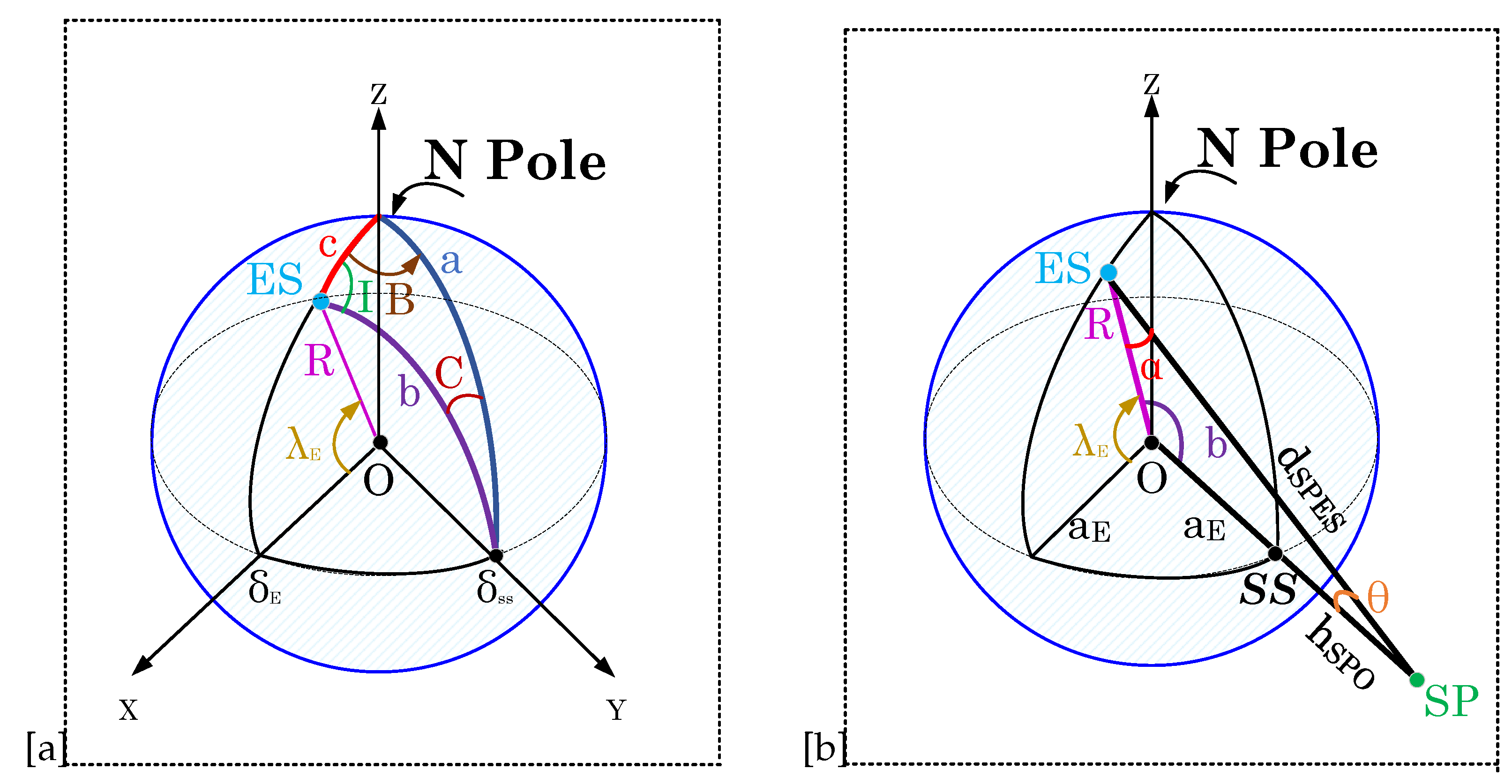
Figure 2.
Uplink satellite geometry for DoA Estimation.

Figure 3.
Downlink satellite geometry for DoA Estimation.

Figure 4.
Uniform Linear Array geometry at satellite systems
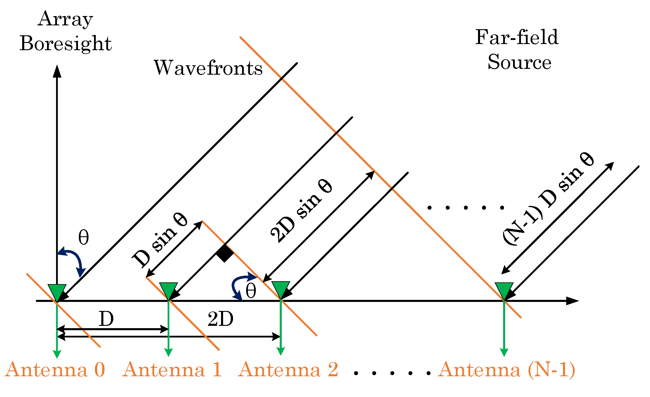
Figure 5.
RMSE performance of uplink Geostationary and Low Earth Orbit satellites using DAS and MUSIC techniques for AWGN only (Case-i(a)).
Figure 5.
RMSE performance of uplink Geostationary and Low Earth Orbit satellites using DAS and MUSIC techniques for AWGN only (Case-i(a)).
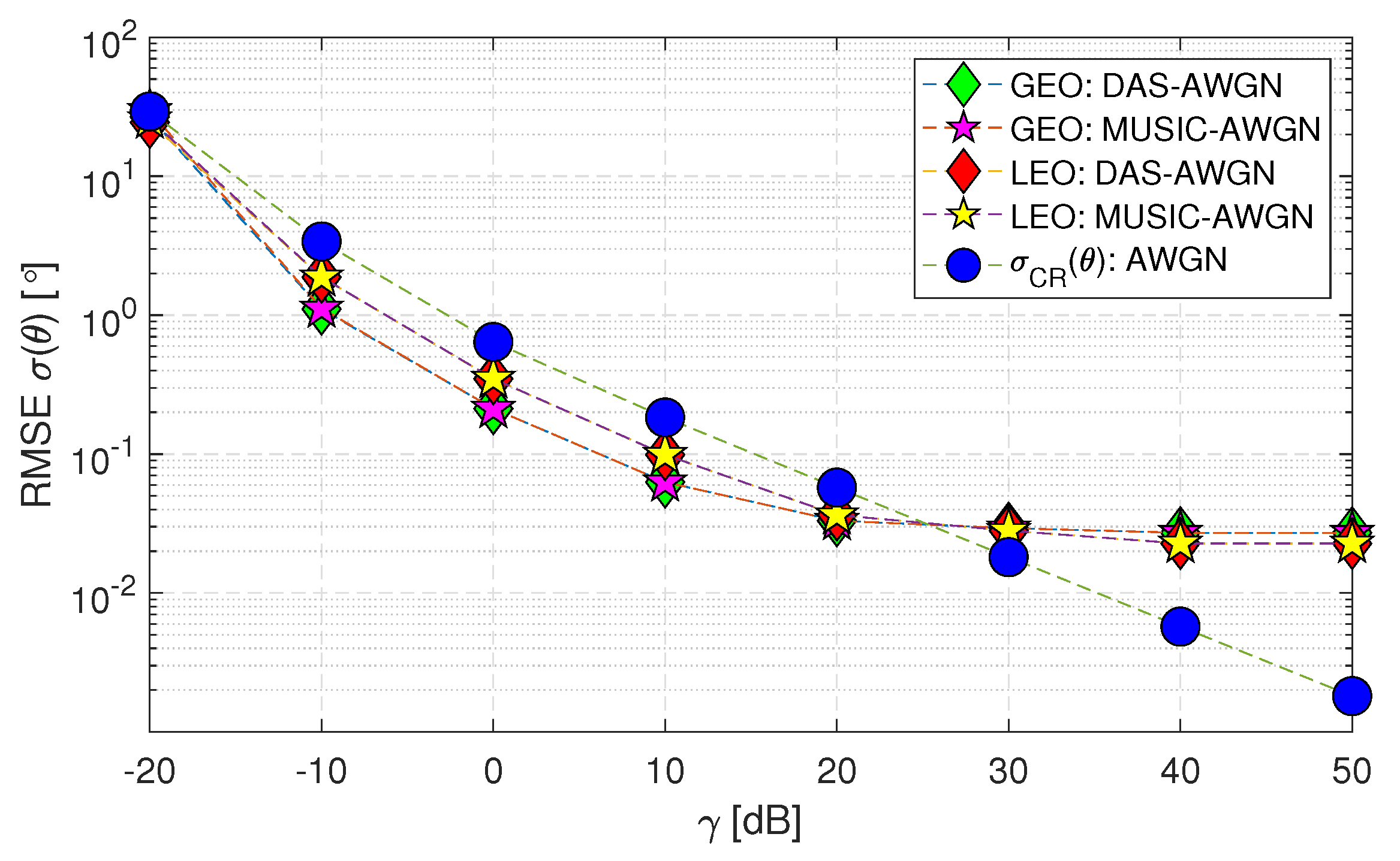
Figure 6.
RMSE performance of downlink Geostationary and Low Earth Orbit satellites using DAS and MUSIC techniques for AWGN only (Case-i(b)).
Figure 6.
RMSE performance of downlink Geostationary and Low Earth Orbit satellites using DAS and MUSIC techniques for AWGN only (Case-i(b)).
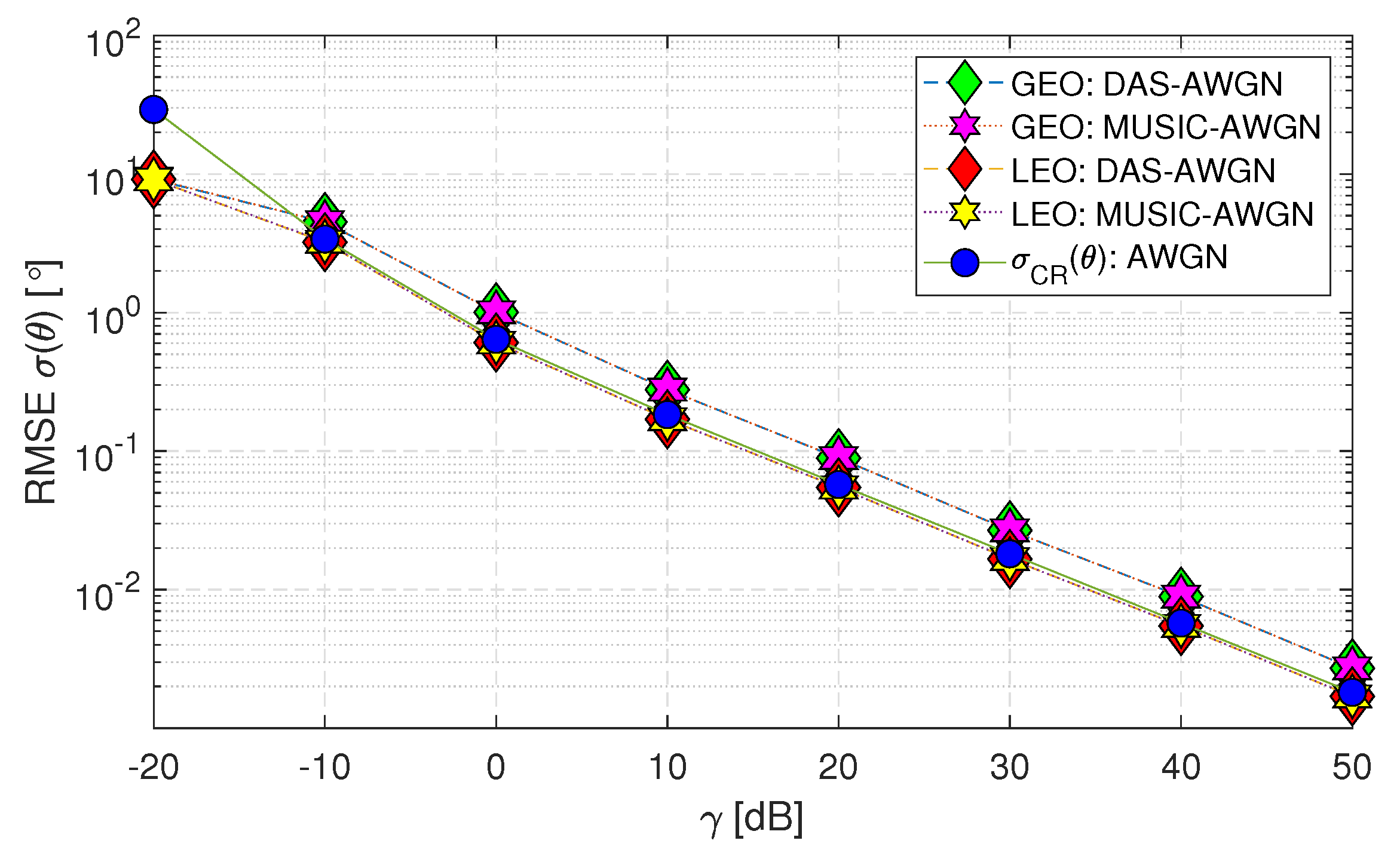
Figure 7.
RMSE performance of downlink Geostationary and Low Earth Orbit satellites using DAS and MUSIC techniques for AWGN and Envelope Fading scenario (Case-ii)
Figure 7.
RMSE performance of downlink Geostationary and Low Earth Orbit satellites using DAS and MUSIC techniques for AWGN and Envelope Fading scenario (Case-ii)
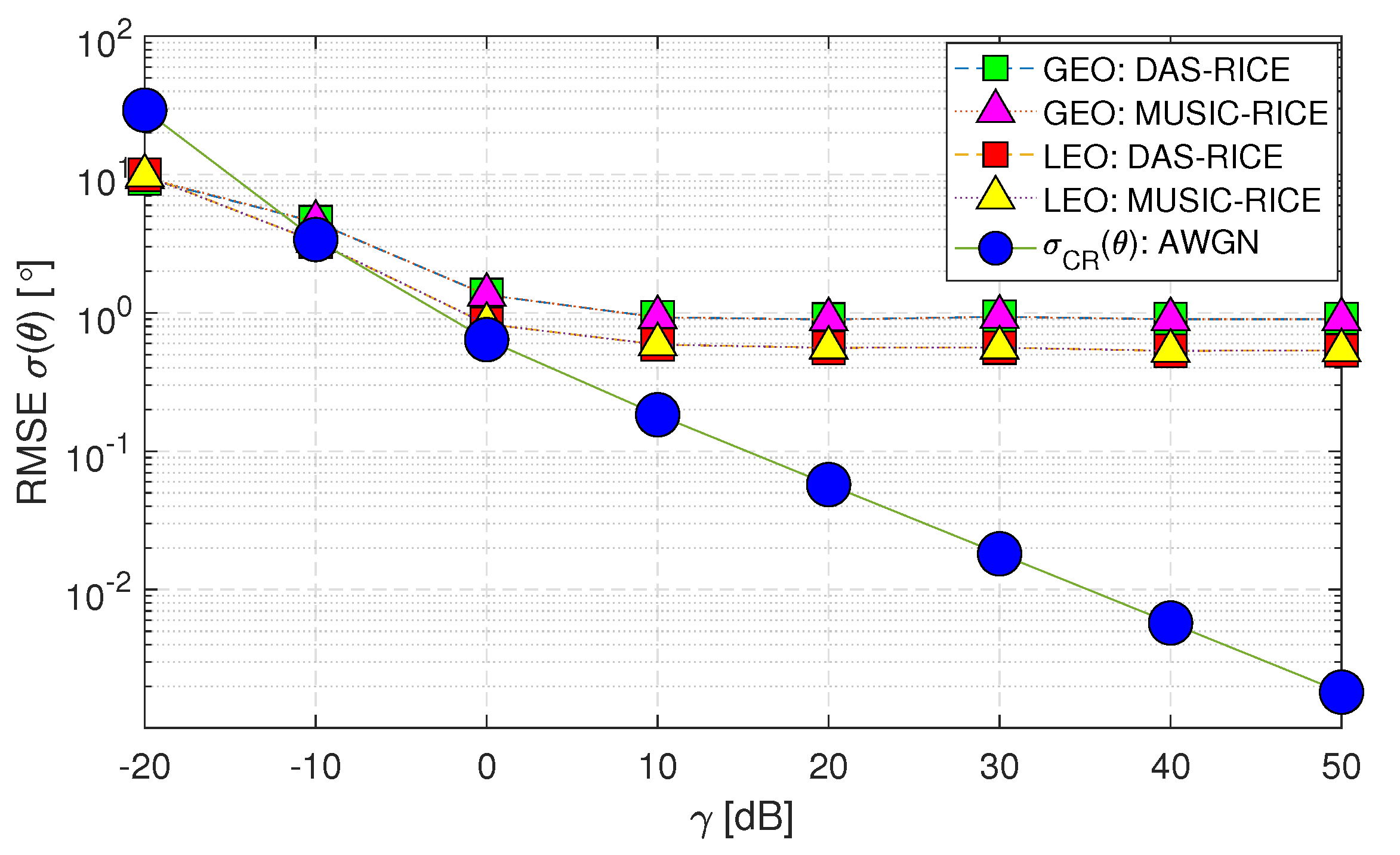
Figure 8.
RMSE performance of downlink Geostationary and Low Earth Orbit satellites using the DAS and MUSIC techniques for spatially correlated channels with AWGN and Envelope Fading (Case-iii).
Figure 8.
RMSE performance of downlink Geostationary and Low Earth Orbit satellites using the DAS and MUSIC techniques for spatially correlated channels with AWGN and Envelope Fading (Case-iii).
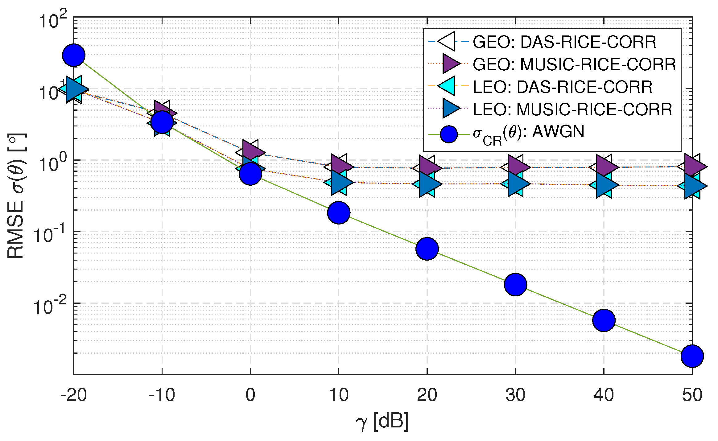
Figure 9.
RMSE performance of downlink Geostationary and Low Earth Orbit satellites using the DAS technique comparing (Case-ii) with (Case-iii).
Figure 9.
RMSE performance of downlink Geostationary and Low Earth Orbit satellites using the DAS technique comparing (Case-ii) with (Case-iii).
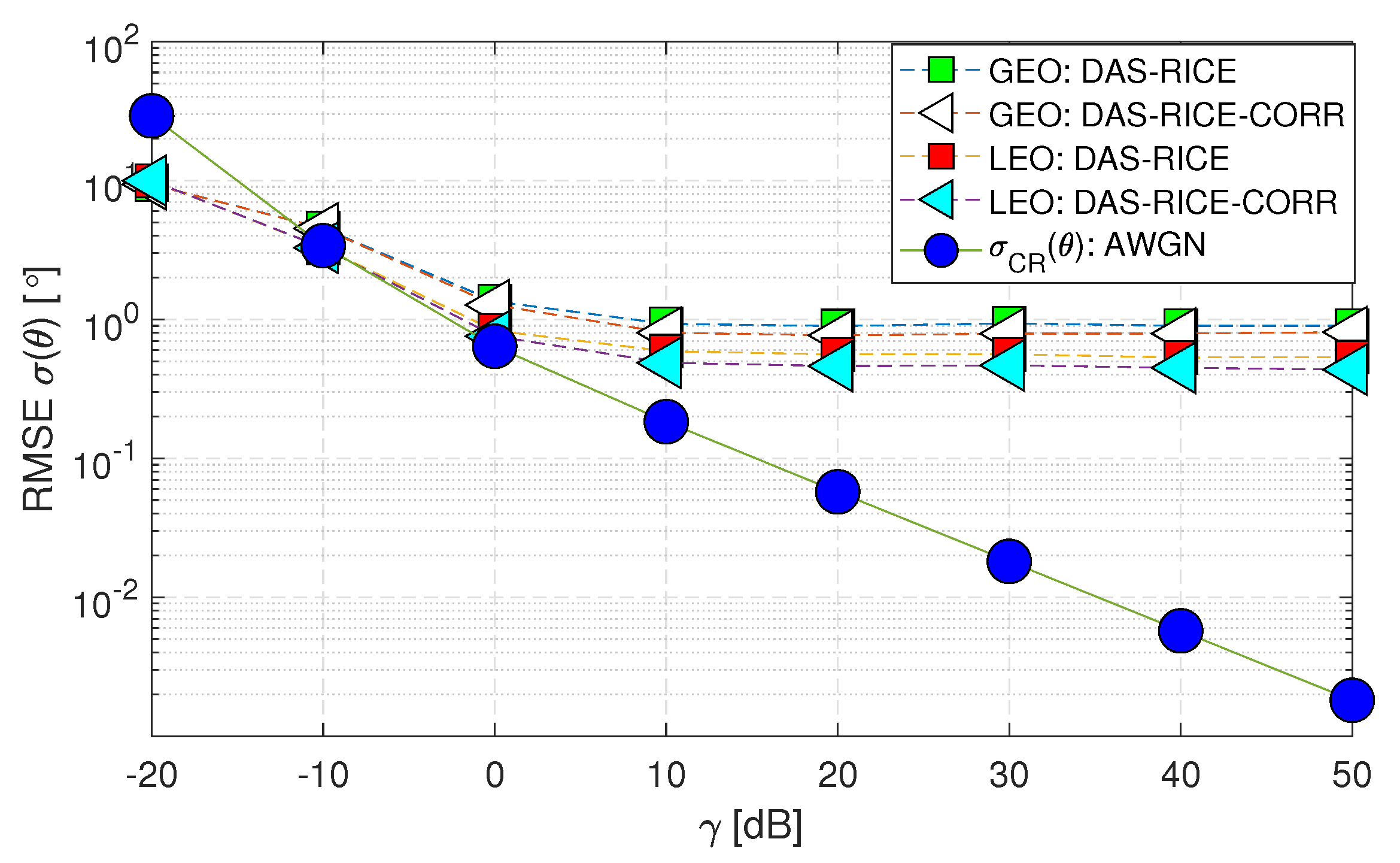
Figure 10.
RMSE performance of downlink Low Earth Orbit satellite using the DAS technique for change in antenna values in spatially correlated channels with AWGN and Envelope Fading (Case-iv).
Figure 10.
RMSE performance of downlink Low Earth Orbit satellite using the DAS technique for change in antenna values in spatially correlated channels with AWGN and Envelope Fading (Case-iv).
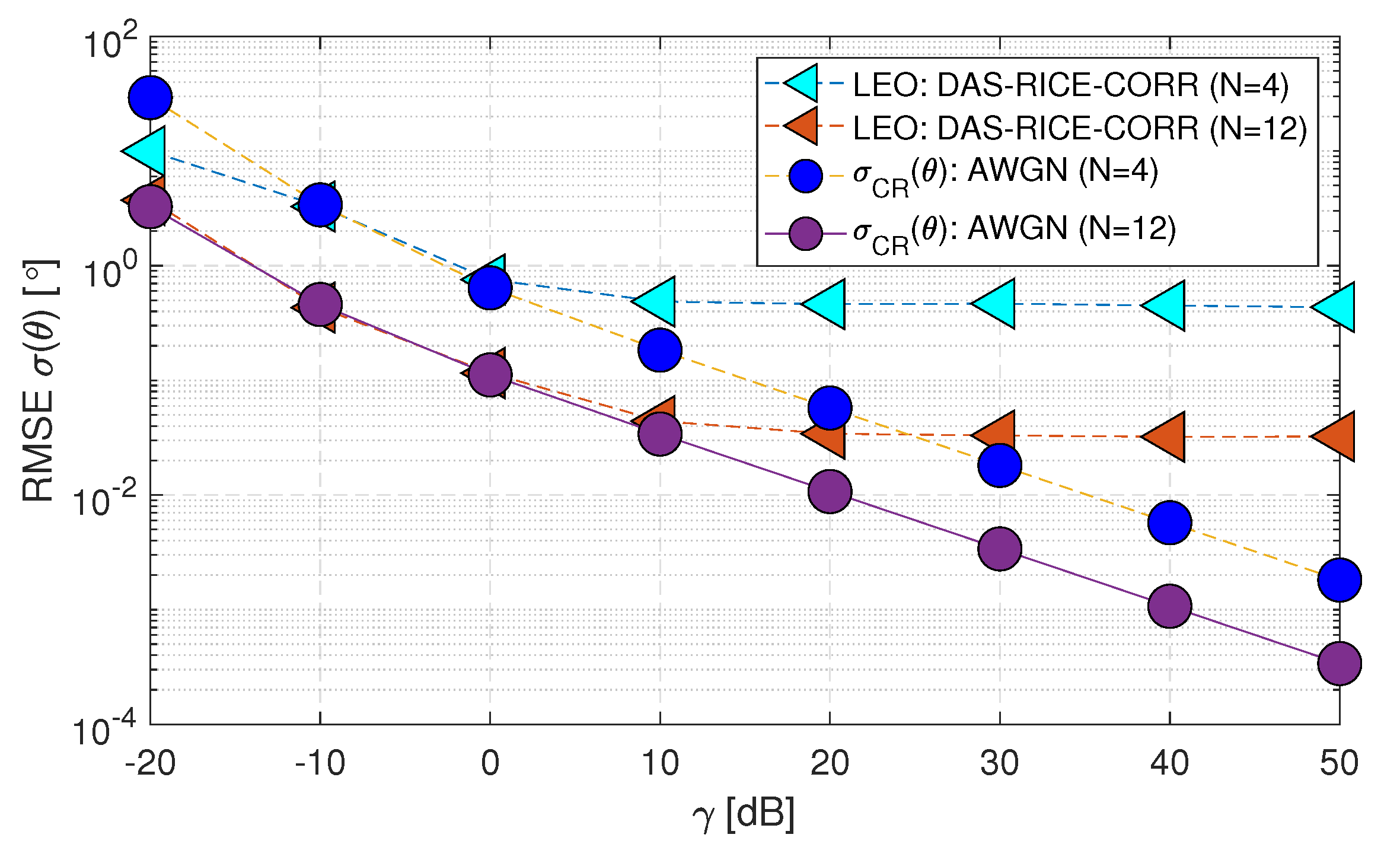
Figure 11.
RMSE performance of downlink Low Earth Orbit satellite using the DAS technique for change in sample sizes in spatially correlated channels with AWGN and Envelope Fading (Case-v).
Figure 11.
RMSE performance of downlink Low Earth Orbit satellite using the DAS technique for change in sample sizes in spatially correlated channels with AWGN and Envelope Fading (Case-v).
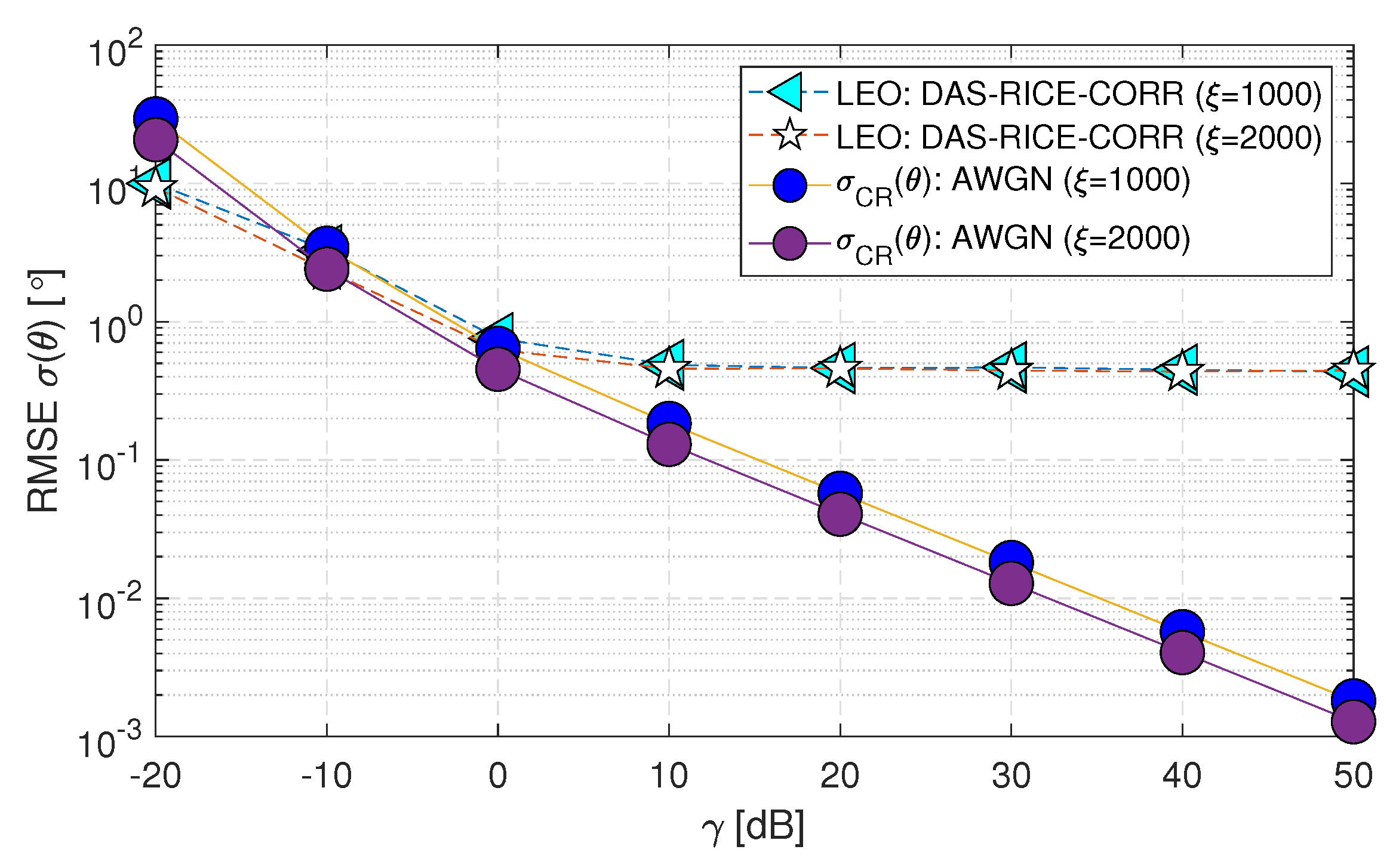
Figure 12.
RMSE performance of downlink Low Earth Orbit satellite using the DAS technique for change in K Factor values in spatially correlated channels with AWGN and Envelope Fading (Case-vi).
Figure 12.
RMSE performance of downlink Low Earth Orbit satellite using the DAS technique for change in K Factor values in spatially correlated channels with AWGN and Envelope Fading (Case-vi).
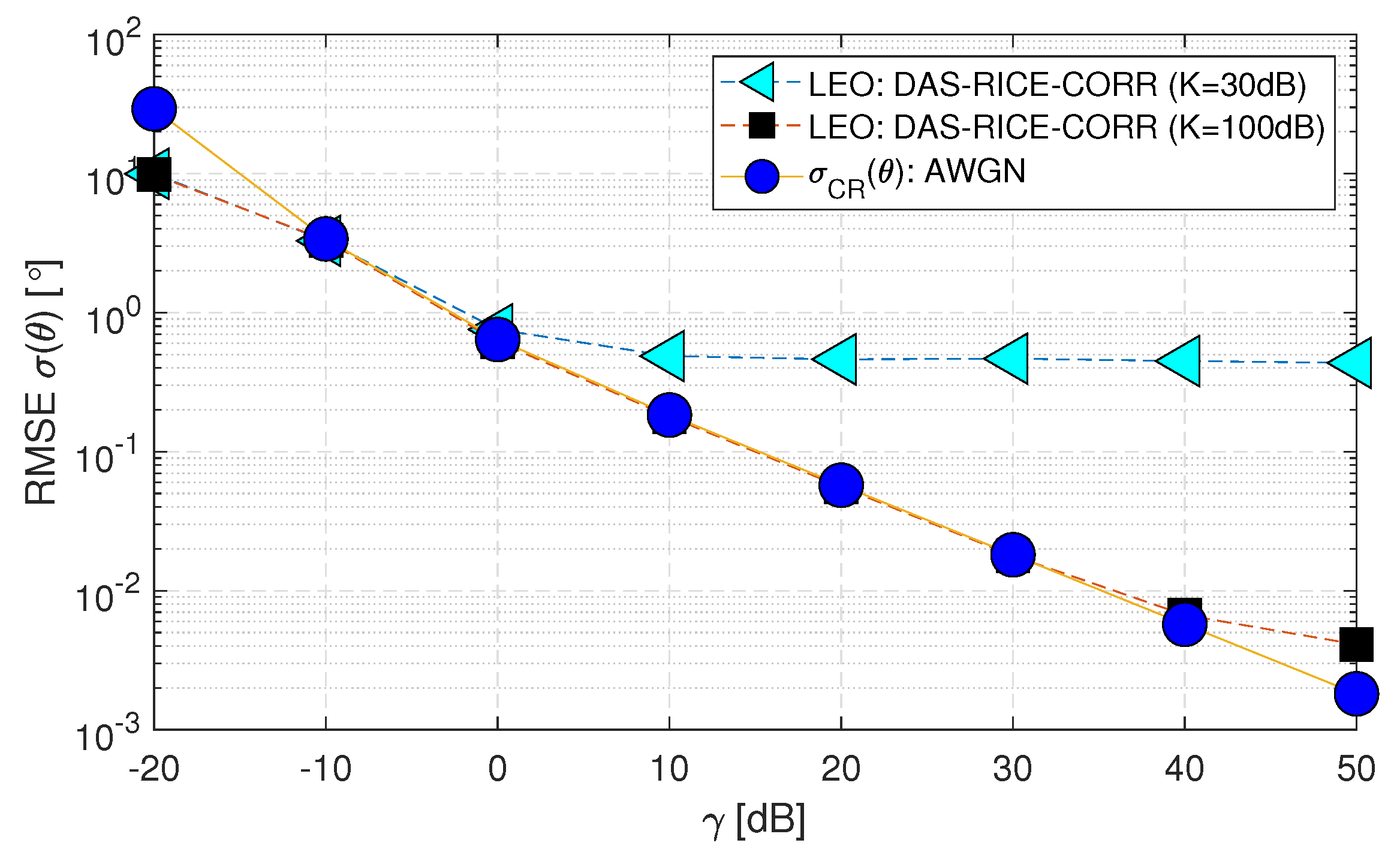
Figure 13.
RMSE of downlink Low Earth Orbit satellite using the DAS technique for changes in De-correlation distance values in spatially correlated channels with AWGN and Envelope Fading (Case-vii).
Figure 13.
RMSE of downlink Low Earth Orbit satellite using the DAS technique for changes in De-correlation distance values in spatially correlated channels with AWGN and Envelope Fading (Case-vii).
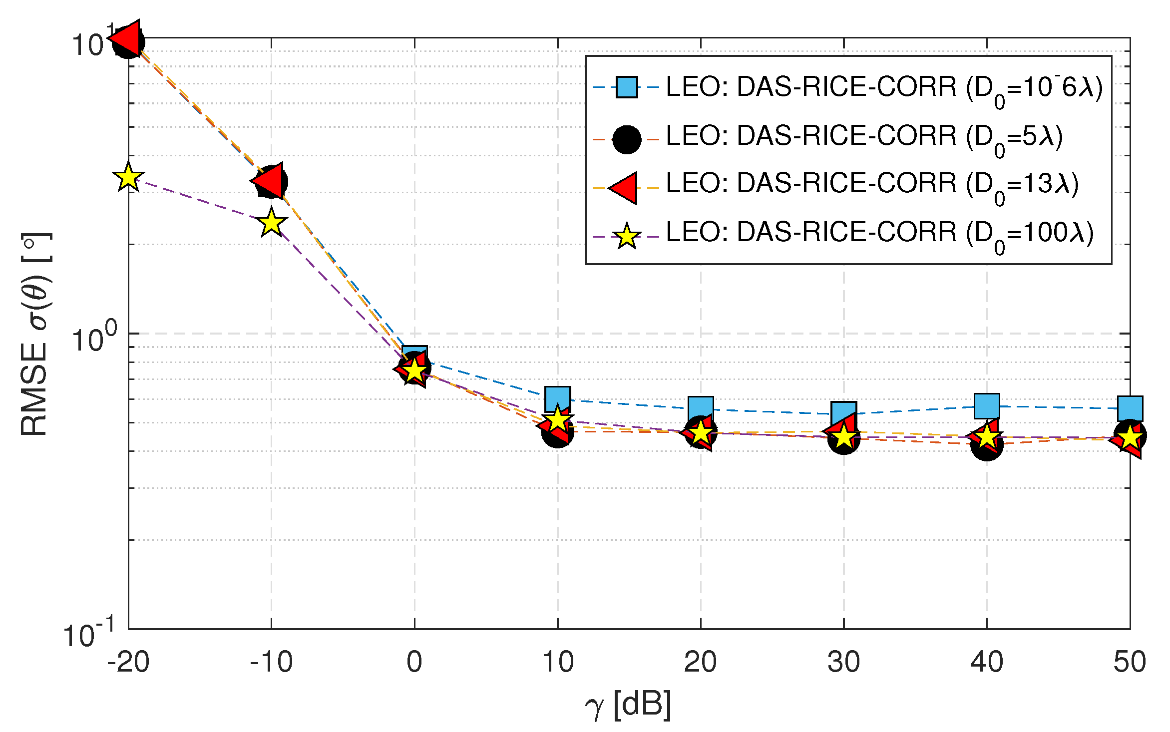

Table 1.
Parameters Table.
| Symbol | Parameter | Units |
| Frequency | 28 [GHz] | |
| Speed of light | 3 [m/s] | |
| N | Antenna values | 4 |
| Signal-to-noise-ratio | (-20 to 50) [dB] | |
| Number of Samples | 1000 | |
| K | Rice factor Value | 30 [dB] |
| De-correlation Distance | 13 at BS | |
| Latitude of Earth Station (Uplink) | - | |
| Longitude of Earth Station (Uplink) | - | |
| Elevation angle of satellites (Uplink) | 10 | |
| Altitude of satellites (Uplink) | 35,786 (GEO) and 1500 (LEO) in [km] | |
| Velocity of satellites | 0 (GEO) and 7.11 (LEO) [km/s] | |
| Velocity Vector’s angle of satellites | 0 (GEO) and 0 (LEO) in | |
| Doppler Shift of satellites | 0 and 663.600 in [kHz] |
Disclaimer/Publisher’s Note: The statements, opinions and data contained in all publications are solely those of the individual author(s) and contributor(s) and not of MDPI and/or the editor(s). MDPI and/or the editor(s) disclaim responsibility for any injury to people or property resulting from any ideas, methods, instructions or products referred to in the content. |
© 2023 by the authors. Licensee MDPI, Basel, Switzerland. This article is an open access article distributed under the terms and conditions of the Creative Commons Attribution (CC BY) license (http://creativecommons.org/licenses/by/4.0/).
Copyright: This open access article is published under a Creative Commons CC BY 4.0 license, which permit the free download, distribution, and reuse, provided that the author and preprint are cited in any reuse.


